Deficits, government expenditures, and tax smoothing in the...

Journal of Monetary Economics 31 (1993) 317-339. North-Holland

Deficits, government expenditures, and tax smoothing in the United States: 1929-1988*

Chao-Hsi Huang National Tsing-Hua University, Hsin-Chu, Taiwan. ROC

Kenneth S. Lin National Taiwan University, Taipei, Taiwan, ROC

Received July 1991, final version received February 1993

Barro’s tax smoothing hypothesis (TSH) implies that the government runs a ‘budget deficit’ whenever it anticipates the growth rate of national income to increase or the growth rate of its expenditure to decline. We test this implication of the hypothesis by examining the implied cross-equation restrictions on a vector autoregression (VAR) model using US. data for the period ranging from 1929 to 1988. Our formal tests reject the hypothesis for the full sample period, but cannot reject it for the post-1947 period. Further investigations show that the statistical rejection should be attributed to sharp differences in the statistical properties of the pre-1947 and the post-1947 data rather than the failure of the hypothesis itself.

Key words: Government expenditures; Tax smoothing hypothesis; Budget deficits

1. Introduction

The ‘tax smoothing hypothesis’ (TSH) championed by Barro (1979) suggests that an optimal tax rule is one which smooths tax rate over time. The idea is that tax collections are distorting and thus should be allocated over time for the sake of minimizing the present value of tax collection costs (excess burdens) for a given expected present value of tax revenues. As shown in Barro (1979), under the condition that the collection cost is an increasing, convex, and time-invariant

Correspondence to: Chao-Hsi Huang, Department of Economics, National Tsing-Hua University, Hsin-Chu 30043, Taiwan, ROC.

*We would like to thank Yih-Luan Chyi, C.Y. Cyrus Chu, Ching-Sheng Mao, and Tsong-Min Wu for helpful discussions. We are also grateful to seminar participants at National Taiwan University, Academia Sinica, and in particular to an anonymous referee for their valuable com- ments. Any remaining errors are ours. Huang acknowledges financial support from the National Science Council of ROC under grant NSCSO-0301-HOO7-13.

0304-3932/93/$06.00 6 1993-Elsevier Science Publishers B.V. All rights reserved

318 C.-H. Huang and K.S. Lin, Testing TSH implications

function of the tax rate, it is optimal for the government to select a uniform tax rate over time such that the expected present value of tax revenues equals that of government expenditures.’ This optimal tax policy has the following observable implications: 1) public debt issue responds positively to temporary increases in government expenditures but responds negatively to temporary increases in aggregate output; and 2) the optimal tax rate is determined by the permanent components of both government expenditures and aggregate output, and temporary changes in these variables should have no effect on the tax rate.

The question of whether the time series properties of U.S. fiscal data are consistent with the above observable implications or not has been previously examined by a number of empirical studies. For example, Barro (1979, 1986a,b) found that the cyclical behavior of U.S. public debt was basically consistent with the first implication. On the other hand, Sahasakul (1986) constructed a series of average marginal income tax rate and found that the tax rate moved with the temporary component of government spending-aggregate output ratio; and the TSH was, as a result, rejected. Despite the fact that Barro and Sahasakul have reached different conclusions, their econometric analyses all require the empirical decomposition of government spending and aggregate output into permanent and temporary components. Inevitably, the validity of their empirical finding hinges upon the specification of variables and equations in their construction of the temporary or permanent components of the series. Further- more, their decomposition procedures could fail to fully utilize the information in the inextricable links between the permanent (trend) and temporary (cyclical) components of the relevant series implied by the model. This possible failure of their procedures would be owing to empirical decomposition only being appropriate whenever determinants of the permanent components are independent of those of the temporary ones.

This paper presents an alternative way of testing the TSH. Our formulation of the tax smoothing model is a standard one. However, log-linearization is employed for reaching an exact linear relation between budget deficit on the one hand and the expected growth rates of government expenditures and aggregate output on the other. This exact linear relation has become the primary focus of our empirical investigation.* This approach has several advantages. First, the

‘In studying optimal taxation over time, the tax smoothing result has also been obtained in different setups by Kydland and Prescott (1980) and Lucas and Stokey (1983).

‘The log-linearization is designed to preserve the additive structure of the closed-form solution of the model, which facilitates our empirical investigation. The closed-form solution of a linear- quadratic version of tax revenue smoothing model has been recently derived and examined by Trehan and Walsh (1988). The U.S. data provide little evidence in the support of such model. However, the tax revenue smoothing model has quite different observable implications from the tax rate smoothing one: for example, the tax revenue smoothing hypothesis implies countercyclical movements of tax rates to occur; the TSH, meanwhile, implies a procyclical pattern of tax revenues. Therefore, empirical results by Trehan and Walsh may not provide useful information as to the validity of the TSH.

C.-H. Huang and K.S. Lirl. Testing TSH implications 319

exact linear relationship has an intuitively appealing economic interpretation. It simply postulates that a higher (lower) current government budget surplus anticipates either a slower (faster) growth of future aggregate income or a faster (slower) growth of future government expenditures. That is, the government saves for rainy days as similarly observed by Campbell (1987) for the behavior of forward-looking households in the permanent income model. Second and more importantly, the approach allows here for direct testing the TSH without any empirical pre-decomposition of relevant data into permanent and temporary components and can consequently prevent any specification error accompanied by inappropriate data decomposition from occurring. A cleaner test is thus accomplished. Also, as a result, the test virtually exploits all relevant information inherent in the relation between the permanent and temporary components of the series considered.

The restrictions imposed by the TSH on the processes of budget deficit (surplus), government expenditure, and aggregate output are the focus of atten- tion here in regard to the empirical investigation of this paper. These restrictions are derived and tested in a vector autoregression (VAR) framework. Using a VAR framework has several advantages. First, as observed by Campbell (1987), cross-equation restriction tests conducted in the VAR framework for a class of exact linear rational expectations models (to which our model belongs) can be transformed into single-equation regression tests. Thus, testing the model in a VAR framework greatly facilitates our empirical investigation. The performance of the TSH can, furthermore, be informally evaluated via a VAR approach in a straightforward way. Restated, by employing unrestricted VAR forecasts of future growth rates of government expenditures and aggregate output, one can construct a series of ‘theoretical’ deficits which are the present values of these forecasts. The actual series of deficit should equal this theoretical series whenever the TSH is correct and no measurement error exists. Deviations of historical values of deficits from the theoretical ones consequently provide an informal measure of the ‘fit’ of the tax smoothing model. This evaluation of the ‘fit’ of the model is an important complement to formal statistical tests since formal tests as the one employed in this paper are often too powerful so that the merits of the model frequently become obscured by statistical rejections3

The rest of the paper is organized as follows. In section 2, a tax smoothing model as that originally formulated by Barro (1979) is set up. Using the log-linearized versions of first-order conditions of the TSH, an exact linear relation is obtained here between current government budget deficit and the expected future growth rates of government expenditures and aggregate output. This linear relation makes it possible to characterize the TSH as a set of restrictions placed upon the trend and cyclical components of government

‘See Cochrane (1989) for an excellent discussion of the issue.


expenditure, aggregate output, and deficit. In section 3, these restrictions are derived in a VAR framework and the methods for formal tests and informal evaluations are described. In section 4, the restrictions in the VAR models are tested through usage of U.S. fiscal data for the period 1929-1988. The informal evaluations of the hypothesis are also conducted. In addition, the relative performance of the TSH is evaluated here against one competing hypothesis on tax rate setting scheme: a scheme which allows for the current income tax rate to positively respond to increases in the current government spending-aggregate output ratio, even when the increases are temporary ones. Contrary to some findings in previous literature [e.g., Sahasakul (1986)], we find no evidence for this tax rate setting scheme and the TSH generally fares better than the scheme in explaining the historical movements of U.S. budget deficit. The last section gives some concluding remarks.

2. Testable implications of a tax smoothing model

A tax smoothing model as that formulated by Barro (1979) assumes that the government minimizes the present discounted value of tax collection costs (or excess burdens), subject to the intertemporal budget constraint faced by it. The cost function is assumed to be time-invariant:

c, = F(T,> YJ =fh) yt, (1)

where C, is the real cost from collecting taxes at time t, T, is the real tax revenue at time t, Y, is the real aggregate output at time t, and r, is the average income tax rate: t, = T,/ Y,. The second equality in (1) follows from the linear homogene- ous property of F() The government is assumed to choose a sequence of tax rates, {zr, t 2 0}, in order to minimize

cc 1 r I[ 1 - r=O 1 +r fbt) yt,

subject to

(2)

where r is the constant real interest rate, G, is the real government expenditure (net of interest payment) at time t, and B, is the real value of government debt held by the public at the beginning of period t. The government is assumed here

C.-H. Huang and K.S. Lin. Testing TSH implicarions 321

to always abstain from inflationary finance. This can be justified by the result of Barro (1982) that the seigniorage accounts for only around 1% to 2% of U.S. government revenue for the post-war period and was nearly zero before 1950. The intertemporal government budget constraint (3) can be derived by ruling out the existence of Ponzi scheme; that is, we assume that lim,, m B,/( 1 + r)f = 0. This condition simply states that public debt cannot grow at a rate faster than or equal to the real interest rate.4

The government is confronted by exogenous sequences of {G,, t 2 0}, ( Y,, t 2 O>, and the stock of public debt at the beginning of period 0 (B,). Given the assumptions that f’ > 0 and f” > 0, it is straightforward to show that minimizing the present value of tax collection costs dictates constant tax rates over time. In the case where the future is uncertain and the collection cost functionf(.) is quadratic, this uniform tax rate rule simply implies that optimal tax rate should follow a martingale process: Etr,+j = t,, for j 2 1. That is, the current tax rate is the optimal forecast of future tax rates. This implication of the hypothesis has been previously investigated by Barro (1981) with no significant evidence against it being found. However, the martingale property of the tax rate process is only one implication of the TSH. It is possible that many tax rate processes satisfy the martingale property but only one of them is consistent with the intertemporal budget constraint (3). Thus, testing the martingale property alone might not be adequate in revealing the strength and weakness of the TSH.

In order to reach a tighter implication of the TSH, both the intertemporal government budget constraint (3) and the uniform tax rate rule must be used in characterizing the time series behavior of fiscal data. Certain approximations are, however, required for reaching a closed-form solution of the model. These approximations involve log-linearizing both the Euler equation and the intertemporal government budget constraint. The log-linearization also provides a more realistic form of model representation since many macroeconomic time series data, including those employed in the current paper, are closer to log- linear than linear.

The log-linearized intertemporal government budget constraint can be derived in three steps. The first step involves log-linearizing the present value of current and future government expenditures:

l-,, = f 1 G,, [ 1

f f=O l+r

4The condition implies, as noted by McCallum (1984), that a constant deficit inclusive of interest payments is consistent with the solvency of the government. Recently, Hamilton and Flavin (1986), Kremers (1989) and Trehan and Walsh (1988) tested this condition and could not reject it using U.S. data. However, see Hansen et al. (1990) for the criticism on the validity of these tests and also some opposing evidence from Trehan and Walsh (1991).

322 C.-H. Huang and K.S. Lin. Testing TSH implications

which implies the law of motion for Tt: Tt+ 1 = (1 + r)(T, - G,), for t 2 0. Dividing the law of motion by T1, taking logarithms on both sides, and using the first-order Taylor’s expansion yields

go - $0 = f $0. - Ast) + ~3 (4) t=1

where go = InGo, Go = In To, Agl = g1 - gt- 1, p is a slightly less than one constant, and y is a constant.5

The second step lies in log-linearizing the present value of current and future tax revenues:

Similar computation gives the following relationship:

to _ to = f p’(r - At,) + Y, 1=1

(5)

where to = InTo, lo = lnQo, and At, = t, - t,_ 1.6 In the final step, assume that B. is strictly positive. The intertemporal government budget constraint (Q. = To + B,) can then be log-linearized as

$0 - 50 = 1 - ; Do - 501 + k, ( 1 where b. = lnBo, Q is a slightly less than one constant, and k is a constant.7 Substituting eqs. (4) and (5) into the above equation for tjo and to, respectively, yields the following log-linearized intertemporal government budget constraint, for t 2 0: ’

30

st = Cd 1

Agt+j- -At,+j , j=l R (6)

5p can be interpreted as the average value of 1 - G/r. See appendix for the detailed derivation of (4).

6Here we made a simplifying assumption that the average value of 1 - T/G is equal to p.

‘CJ can be interpreted as the average value of 1 - B/G.

sThe constant term is dropped here since the model will be fitted with the demeaned time series data.

C.-H. Huang and K.S. Lin. Testing TSH implications 323

where 1 1-Q

s, = 2t, - gt - S2b,.

Suppose that the optimal tax rate rule under uncertainty can be approximated reasonably well by E, Ins, +j = lnr,, for j 2 1. Linearly projecting both sides of eq. (6) onto the relevant information set at time t, which includes at least s,, and substituting the approximated optimal tax rule into the resulting equation yields the final expression:

where y, = lnY,. This equation reflects that there exists an exact linear relation across current realization of ‘budget surplus’ (s,) and the forecasts of all future growth rates of aggregate output and government expenditures.’ The equation also posits the following observable implications of the TSH for the ‘budget surplus’ movements. First, the budget surplus becomes higher (lower) whenever the government anticipates either a faster (slower) growth of government spending or a slower (faster) growth of aggregate output. Hence, the government also saves for rainy days, as is similarly true for rational forward-looking households in the permanent income model. To elaborate more on this implication of eq. (7), consider a case where the government expenditures are expected to grow slower than normal in the future as the temporarily high government expenditures begin to return to the normal trend. In this case, the optimal policy of the government, according to (7), lies in smoothing out tax rate and running a higher (lower) than normal current budget deficit (surplus). Therefore, temporary high government expenditure would lead to an increase in public debts. In contrast, consider another case where the aggregate output has reached its peak in business cycle fluctuations. In this case, slower than normal growth of aggregate output is expected, which in turn, according to (7), indicates that the government would smooth out tax rate and run a higher than normal current budget surplus. Thus, a temporarily high aggregate output would result in a lower level of government debts. These implications of the TSH have been previously stressed by Barro (1979). Finally, (7) also implies that the current surplus would not respond to any change in government expenditures or aggregate output as long as the present discounted value of the expected growth rates of the latter two series is not affected by the change.

‘The ‘budget surplus’ here is (I/Q)t, - y, - (1 - Q)b,/R, which is not as that conventionally defined. However, this definition has similar characteristics as the conventional counterpart. That is, it increases with a rise in T, and decreases with an increase in G, or E,.

324 C.-H. Huang and KS. Lin, Testing TSH implications

3. The VAR method

Following the empirical strategy for the study of exact linear rational expectations models proposed by Campbell (1987), we test the linear relation (7) in a VAR framework. Suppose that gt and y, are both difference-stationary, then (7) implies the stationarity of s,. Given the stationarity of s,, Ag,, and Ay,, provided that gt and y, are not cointegrated, the following VAR(p) model for X, = [s,, Agt, AyJ’ should exist:

x, = C(L)X,- 1 + u,, (8)

where C(L) = Co + C,L + ... + C,_lLp-l, with C, being a 3 x 3 coefficient matrix, and u, is a 3 x 1 vector white noise process.” System (8) can be stacked here to form: Z, = AZ,_r + U,, where Z, = [s,, . . . . s,_~+~, Ag,, . . . , Agt-p+l, Ay,, . . , by, _p+ J’ is a 3p x 1 vector of random variables, A is the corresponding companion matrix, and Ui, is the 3p x 1 white noise vector. Notice that the optimal forecast of Z, i periods ahead given {Z,, Z,_ 1, . . . } should satisfy E,Z,+i = A’Z,, for i 2 1. This formula makes it easy to translate eq. (7) into the following expression:

I’z, = f (h’ - k’w ‘) piAiZ,, i=l

(9)

where 1, h, and k are column vectors with 3p elements, all of which are zero except for the first element of 1, the p + 1st element of h, and the 2p + 1st element of k, which are one. Since p and the eigenvalues of A are all less than one in absolute value under current specification and since eq. (9) holds for any realization of Z,, we have I’ = (h’ - k’K’)pA(I - PA) -’ or:

I’(1 - ,oA) = (h’ - k’S2- ‘)pA,

where I is a 3p x 3p identity matrix. The above equality places a set of linear restrictions on the coefficients in matrix A. These restrictions can be shown to simply reflect that the realizations of stmi, Agtmi, and AY,_~, for i = 1,2, . . . , p,

do not have marginal predictive power over the movement of s, + Agr - Q- ’ Ayt - p- ‘s, _ 1. Testing the linear restrictions on the coefficients

“If y, and q, were cointegrated with cointegrating vector (1, - a), then a model consisting of s,, Ag,, and Ay, would be a overdifferenced system. As a result, the moving average representation of the model could not be inverted and hence the VAR representation does not exist. To have a VAR representation, in this case, an appropriate set of variables would be s,, y, - ag,, and by,. A more detailed discussion about the link between the cointegration and the noninvertible vector moving average representation of an overditferenced system is provided in Engle and Yoo (1987).


in matrix A consequently becomes a simple regression test.” One important feature of this testing method is that, unlike the empirical strategy taken by Barro (1979, 1986a,b) and Sahasakul (1986), it does not require any empirical pre-decomposition of government expenditures and aggregate output into permanent and temporary components. As a result, it avoids any possible error caused by data decomposition.

The above VAR model can also be used for informally evaluating the performance of the TSH. Specifically. a series of ‘theoretical’ budget surplus denoted as ST can be constructed here, which is the optimal VAR forecast of the present value of future growth rates of aggregate output and government expenditures. Since s, is included in the current information set, according to (7) under the TSH s: should differ from s, only by sampling error. As a result, comparisons between s, and sf provide an informal way of evaluating the economic performance of the TSH. This evaluation becomes useful whenever the regression test turns out to be too powerful in the case under consideration.

4. Data and empirical results

The data on federal expenditures, net federal interest payments, federal receipts, GNP, and implicit GNP price deflator are taken from National Income

and Producr Accounts (NIPA); the data on the end-of-calendar-year par value of privately held interest-bearing federal debt are taken from statistical tables in various issues of the Economic Report of the President. All data are annual series for the period 192991988. The following adjustments are executed to make the data series compatible with the theoretical definitions. First, net federal interest payments are subtracted from federal expenditures since G, defined above does not include interest payments. Second, a portion of interest payments made by the Treasury to the Fed, which were returned to the Treasury, are counted as the Treasury receipts. We subtract these returned interest payments from the federal receipts. Third, notice that B, is defined as the beginning-of-period value of public debts in (3). The end-of-last-calendar-year public debt series is used here as a substitute since the beginning-of-calendar-year series is not available. Fourth and finally, all nominal data series are deflated by the implicit GNP deflator for the sake of constructing the real data series.

The evolution of Agt and Ay, over the period of 1929-l 988 is depicted in fig. 1. Three characteristics of these series are worth mentioning. First, the Agt series exhibited volatile movements during wartime periods and it was more volatile during World War II than during the Korean and Vietnam wars. These volatile

“Similarly. it can be shown that once Y, and y, are cointegrated with cointegrating vector (1, -a), the cross-equation restrictions can be tested by regressing s, + Ag, - (I/Q)Ay, - (l/p)s,_, on lagged values of s,, y, - xg,, and Ay,.

326 C.-H. Huang and KS. Lin, Testing TSH implications

1.5

-1.5 / I I I II I, / I I / I, I/ I ,I ,I/ I I,,, I,, I,, I,,, , I, I, I,,, ,, ,I,#, ,, / ,, I 1930 1935 1940 1945 1950 1955 1960 1965 1970 1975 1960 1965

Year

Fig. 1. Growth rates of government expenditure and GNP, 193&1988. The growth rate of G, is marked by -~- and the growth rate of Y, is marked by -.

movements in Ag, primarily reflected the drastic changes in war expenditures occuring during those periods. Significant increases in Agr also occurred in recession periods, particularly during the Great Depression and the two post- war major recessions (1974-75 and 1980-82); the fluctuations were more drastic during the Great Depression than during the post-war recessions. Second, the by, series was substantially smoother than the Agt series over most of the period 192991988. Third and finally, the statistical properties of Ag, and Ay, for the period 192991946 appear to differ from those for the period 1947-1988. This visual impression is also supported by relevant sample statistics: (1) the respective sample means of Agl and Ay, are 15.0% and 2.5% for the period 1930-1946, while they are a respective 3.6% and 3.1% for the post-war period; and (2) the respective sample standard deviations of Ag, and Ayt are 46.4% and 11.5% for the former period, but are only a respective 9.5% and 2.7% for the latter.

The results of the unit root and the cointegration tests for g1 and y, processes are reported in table 1. The tests are important preliminaries because the inclusion of Agr, Ayr, and s, as the variables in (8) is appropriate only if 1) both gt and y, are difference-stationary and 2) y, and gt are not cointegrated; that is, they contain two distinct unit roots. Panel A presents the test statistics in Dickey-Fuller (1979) regression with and without a linear time trend. The former is appropriate when the alternative hypothesis is that the series is stationary around a linear time trend, the latter when the alternative is that the series is stationary around a constant mean. The results show that the null

C.-H. Huang and K.S. Lin, Testing TSH implications 327

Table 1.

Unit root and common trend testsa

Variables

St

Yr Agr A)‘f s, (0 = 0.96)

(Q = 0.97)

(Q = 0.98)

(a = 0.99)

YI

Yr A.q,

AI’, s, (Q = 0.96)

(Q = 0.97)

(_Q = 0.98)

(0 = 0.99)

(A) Unit root tests

Ho: The series contains a unit root. H,: The series is stationary.

Period 1929-88 Period 1947-88

With trend Without trend With trend Without trend __~

Dickey-Fuller tests: r-statistics

- 2.59 - 2.64 - 3.39 - 2.55

- 2.45 - 0.05 - 2.30 - 1.24

- 5.19’ - 5.09’ - 5.35’ - 5.08’

-- 4.35’ - 4.41’ - 5.39’ - 5.36’

- 4.53’ - 4.07’ - 5.83’ - 5.30’

- 4.52’ -4.11’ - 5.79’ - 5.23’

- 4.51’ - 4.15’ - 5.79’ - 5.16’

- 4.50” - 4.18’ - 5.76’ - 5.08’

Phillips-Perron tests: Z(t,)-statisticP

- 2.83 - 2.54 NA - 2.68

- 1.99 - 0.28 NA - 1.31

- 4.64” - 4.27’ - 5.95’ - 5.33’

- 4.64’ - 4.31’ - 5.91’ - 5.27’

- 4.63’ - 4.35’ - 5.97’ - 5.21’

- 4.62’ - 4.38’ - 5.95’ - 5.15’

- 5.14’ - 5.07’ - 5.28’ - 4.96’

- 4.21’ - 4.53’ - 5.40’ - 5.27’

(B) Stock-Watson common trend tests for g, and y,: &-statistics

H,: Number of unit roots is two. H,: Number of unit roots is one.

Period 1929-88 Period 1947-88

Lag length Qf p-value QJ p-value

1 - 9.98 23.75% - 4.32 63.00% 2 - 8.19 33.25% - 3.35 71.75% 3 - 8.28 32.50% - 3.69 68.50% 4 - 6.73 42.75% - 1.03 92.00%

“The variables are y, = real federal noninterest outlays, yt = real GNP, all in natural logarithms,

and s, = (l/Q) f, - g, - [(1 - n)/UJb,. where t, = real federal receipts and b, = real privately held

interest-bearing federal debt at the end of the last period, all in natural logarithms. The A’s refer to

first differences. Annual data are used. bTo construct Phillips and Perron test statistics, we use third-order window and the weighting

scheme of Newey and West (1987). In the ‘with trend’ case the test statistics for the g, and y, series for

the 1947-88 period are not reported because the resulting values are not defined.

‘Rejection of the null hypothesis at the 5% level.

328 C.-H. Hung and KS. Lin, Testing TSH implications

hypothesis that gt (or y,) contains a unit root cannot be rejected at the 5% level for the full sample and the post-war periods. The Phillips and Perron (1988) test is also conducted here so as to account for possible autocorrelation or hetero- scedasticity of regression residuals.” This test is indicated in panel A to generally yield results similar to the Dickey-Fuller one.13 The Stock and Watson (1988) common trend test results are reported in panel B. The test fails to reject the null hypothesis of g1 and y, containing two independent unit roots at 5% level for both full and short sample periodsI

To conduct formal tests, an appropriate order must first be selected for the VAR model (8) and the values for 52 and p must be specified. According to the Schwarz information criterion, the optimal order is selected to be one for both the full and short sample periods. The values chosen for Q and p depend on the sample period investigated. The values for the period 1929-1988 are assumed to be 0.97 and 0.98, respectively.”

The cross-equation restrictions of the TSH for the VAR( 1) specification can be translated into three zero restrictions on the coefficients in the following regression equation (a, = a2 = a, = 0):

s, + Ag, - Q-‘Ay, - p-lst-r = a0 + a,~,_, + aZAg,_,

+ aJAy,-, + E,. (10)

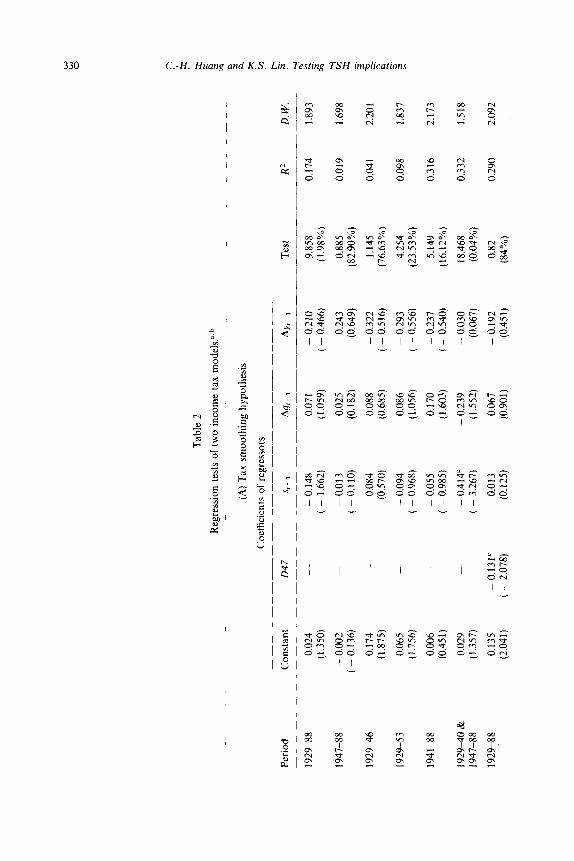
For the sake of addressing the potential heteroskedasticity problem in E,, we run regression tests with White’s (1980) correction for heteroskedasticity. The heteroskedasticity-consistent Wald test statistics, which measure the joint predictive power of s,_ 1, Ag,_ 1, and Ay,_ 1 over the dependent variable, and estimates of (10) along with the heteroskedasticity-consistent r-statistics are reported in panel A of table 2.’ 6 Line 1 and line 2 show that the TSH is rejected

“More detailed discussions are provided in Phillips (1987) and Phillips and Perron (1988).

130ne weak implication of the TSH is that the stationarity of Ag, and Ay, implies the stationarity of s,. As indicated by the results in panel A, the data are generally supportive of this implication under various values of 62.

r4We have also conducted the augmented Dickey-Fuller (ADF) test suggested by Engle and Granger (1987) to test the cointegration of g, and y,. The results, which are not reported here, are consistent with Stock-Watson common trend test results, except for the post-war period. Thus, when testing the TSH for the post-war period, we also investigate the case where the cointegration of gr and y, is assumed. The results, which are available upon request, are similar to those reported in table 2.

15p is calculated as the sample mean of 1 - T/O and C2 is the sample mean of I - B/@. To get @ series for the period 1929-1988, we assume that the real interest rate is 4% and the expected long-term growth rate of the real tax revenue is 2.93%, which is the average growth rate of the real GNP over the period. We have found that the test results are not sensitive to the values chosen for p and R.

16The heteroskedasticity-consistent Wald test statistic is pZ-‘b, where @ is the vector of coefficient estimates and Z is the consistent estimate of the covariance matrix of the coefficients allowing for possible heteroskedasticity. The statistics are x2 (3) distributed.


for the period 1929-1988, but cannot be rejected for the post-war period. The rejection for the 1929-1988 sample is quite puzzling, since drastic and presum- ably temporary changes in government spendings during the Great Depression and World War II appear to be perfect opportunities to smooth tax rates. In light of these results, series of regressions are run to examine how the results depend on the sample period chosen. Line 3 and line 4 report the results from the pre-1947 and the pre-1953 data, respectively. For both sample periods, the TSH cannot be rejected. However, as line 5 and line 6 indicate, whenever the post-war period data are combined with those from either the Great Depression or the World War II period, the evidence is less supportive for the TSH. Finally, unstable estimates, especially for the intercept term, across various sample periods indicate that the regression relationship might have changed over time. Since the unstable intercept term might have affected our test results, we run a regression including a dummy (denoted 047) to capture the possible mean shift of the regressand between the pre-47 and the post-47 periods, As line 7 shows, the mean shift of the regressand between the two periods is quite significant. More importantly, all regression coefficients (except those for the constant term and the dummy) now become insignificantly different from zero, and hence the TSH cannot be rejected for the entire period sample. These evidences point toward the direction that differences in the data-generating process across different subsample periods rather than the failure of the TSH itself should account for the statistical rejection for the full sample period data.i7

The questions remaining to be answered are whether there were really significant changes in the data-generating processes of s,, Agl, and Ay,, and when the actual time of the changes was if they did occur. In answering these questions, the multivariate CUSUM technique [e.g., Han and Park (1989)] is used here for identifying possible structural breaks in the underlying data- generating processes. To do so, an unrestricted version of VAR(l) model (8) is first estimated for the period 1929-1937, and then recursive residuals are generated by the period-by-period inclusion of annual observations into the estimation process. The cumulative sums of these residuals for the period 1938-1988 are plotted in fig. 2. As is visually apparent, the plot shows no sign of structural instability up to 1947, and then the cumulative sum of residuals for the Agl equation exhibits a definite downward trend, suggesting a structural break around 1947. The downward trend in the cumulative sum of residuals for the Ag, equation reflects that the VAR model estimated using pre-1947 data consistently overpredicts the post-1947 Ag,‘s. This result accords well with the data characteristics of the Ag, series: the pre-1947 Ag,‘s were on average much higher than their post-1947 counterparts (the sample mean is 15% for the former

“Regressions are also run here with the lag length of the regressors equal to two. The results, which are not reported, are similar to those in table 2.

Tab

le

2

Reg

ress

ion

test

s of

tw

o in

com

e ta

x m

odel

s.“.

b ~_

_~~_

~_~

___~

____

_~__

(A)

Tax

sm

ooth

ing

hypo

thes

is

Coe

ffic

ient

s of

reg

ress

ors

Peri

od

Con

stan

t 04

7 St

-1

AY

,-,

Tes

t R

Z

1929

-88

0.02

4 -

0.14

8 0.

07 I

-

0.21

0 9.

858

0.17

4 (1

.350

) ( -

1.

662)

( 1

.059

) ( -

0.

466)

(1

.98%

)

1947

-88

- 0.

002

- 0.

013

0.02

5 0.

243

0.88

5 0.

019

(-

0.13

6)

( - 0

.110

) (0

.182

) (0

.649

) (8

2.90

%)

1929

46

0.17

4 0.

084

0.08

8 -

0.32

2 1.

145

0.04

1 (1

.875

) (0

.570

) (0

.685

) ( -

0.

516)

(7

6.63

%)

1929

-53

0.06

5 -

0.09

4 0.

086

- 0.

293

4.25

4 0.

098

(1.7

56)

( - 0

.968

) (1

.056

) ( -

0.5

56)

(23.

53%

)

1941

-88

0.00

6 -

0.05

5 0.

170

- 0.

237

5.14

9 0.

316

(0.4

51)

( -

0.98

5)

(1.6

03)

( - 0

.540

) (1

6.12

%)

1929

40

&

0.02

9 -

0.41

4’

- 0.

239

- 0.

030

18.4

68

0.33

2 19

47-8

8 (1

.357

) ( -

3.

267)

(1

.552

) (0

.067

) (0

.04%

)

1929

-88

0.13

5 -

0.13

1’

0.01

3 0.

067

- 0.

192

0.82

0.

290

(2.0

41)

( -

2.07

8)

(0.1

25)

(0.9

01)

(0.4

5 1)

(8

4%)

2.20

1 3 2 ;:

1.83

7 $

2.17

3

1.51

8

2.09

2

___

_~__

__

(B)

Inco

me

tax

sche

me:

7,

=

f!(G

JY,)

p

Coe

ffic

ient

s of

reg

ress

ors

P

0.3

Peri

od

___~

_ 1929

46

Con

stan

t

0.03

1

(0.4

18)

s,-

1 A

&1

AY

,-,

Tes

t R

2 D

. W.

~~

__

___

- 0.

241

- 0.

082

- 0.

461

5.60

1 0.

217

2.54

7 ( -

1.

864)

(

- 0.

810)

( -

1.

012)

(1

3.27

%)

0.3

1947

-88

0.00

1 (0

.042

)

0.5

1929

46

- 0.

064

( -

0.94

0)

0.5

1947

-88

0.00

3 (0

.125

)

0.7

1929

46

- 0.

159

( -

2.25

3)

0.7

1947

788

0.00

4

- 0.

185

( -

1.64

0)

- 0.

458’

(-

3.

100)

- 0.

300

( -

2.57

4)

- 0.

674’

( -

3.

687)

- 0.

414’

( -

0.01

4 0.

194

- 0.

084)

(0

.412

)

- 0.

195

- 0.

555

- 1.

772)

(-

1.

300)

- 0.

040

0.16

1 -

0.20

6)

(0.2

97)

- 0.

308’

-

0.64

8 -

2.23

3)

( -

1.34

6)

- 0.

066

0.12

8

3.16

5 0.

067

1.58

2 (3

6.69

%)

16.4

09

0.42

2 2.

599

(0.0

9%)

10.5

69

0.14

5 1.

516

(1.4

3%)

20.4

34

0.51

6 2.

498

(0.0

1%

)

22.8

49

0.21

6 1.

466

(0.1

88)

( -

3.33

4)

( -

0.30

0)

(0.2

07)

(0.0

04%

) -_

__

~__~

__

_~__

~~

“The

de

fini

tions

of

re

gres

sors

ar

e as

de

scri

bed

in

tabl

e 1

(with

04

7 de

notin

g a

dum

my

vari

able

w

ith

valu

e ze

ro

for

the

pre-

1947

pe

riod

an

d on

e ot

herw

ise)

. T

he

regr

essa

nd

is S

, +

AY

, -

R-‘

Ay,

-

p-Is

,_,

for

the

regr

essi

ons

in p

anel

A

and

s,

+

(1 -

p/

Q)A

g,

- [(

1 -

/J)/

Q]A

y,

- p-

is,_

1

for

the

re-

gres

sion

s in

pan

el

B,

whe

re

Q a

nd

p ar

e eq

ual

to 0

.97

and

0.98

, re

spec

tivel

y.

The

nu

ll hy

poth

esis

te

sted

in

pan

el

B i

s th

e in

com

e ta

x sc

hem

e:

1, =

B

(G,/Y

,)fi

, w

here

r,

= av

erag

e in

com

e ta

x ra

te,

0 is

a c

onst

ant,

G,

= re

al

fede

ral

noni

nter

est

outla

ys,

and

Y, =

re

al

GN

P.

Ann

ual

data

ar

e em

ploy

ed.

“In

pare

nthe

ses

belo

w

each

co

effi

cien

t ar

e r-

stat

istic

s co

nstr

ucte

d by

usi

ng

hete

rosk

edas

ticity

-con

sist

ent

stan

dard

er

rors

. T

est

is t

he h

eter

oske

dast

icity

- co

nsis

tent

W

ald

test

of

the

hy

poth

esis

th

at

all

regr

essi

on

coef

fici

ents

ex

cept

th

e co

nsta

nt

are

zero

. In

pa

rent

hese

s be

low

ea

ch

Wal

d te

st

stat

istic

is

the

co

rres

pond

ing

sign

ific

ant

leve

l, D

. W.

is t

he

Dur

bin-

Wat

son

stat

istic

. ‘R

ejec

tion

of t

he

null

hypo

thes

is

that

th

e co

effi

cien

t is

equ

al

to

zero

at

th

e 5%

le

vel.

332 C.-H. Huang and KS. Lin. Testing TSH implications

30

20 i

lo 5% significance line

1937 1942 1947 1952 1957 1962 1967 1972 1977 1962 1967 Year

Fig. 2. CUSUM of recursive residuals, 1937-1988. The values of CUSUM of residuals for Ag, are marked by L, the values of CUSUM of residuals for Ay, arc marked by -, and the values of

CUSUM of residuals of s, are marked by

and only 3.6% for the latter). I8 The significance lines drawn in the CUSUM plot are, according to Brown et al. (1975), best regarded as ‘yardsticks’ against which to assess the observed residual path rather than in providing a formal test of significance. A formal test is therefore also employed here for verifying the possible structural break of the joint data-generating process of s,, Ay,, and Agl around the year 1947. The formal likelihood ratios test produces a ~‘(12) statistic of 37.2 against a 5% critical value of 21.0, and thus firmly rejects the null hypothesis of no structural break of the process in the year 1947.19

‘sNotice that the usage of multivariate CUSUM technique requires orthogonal residuals. Thus, the CUSUM plot depends on the ordering of the variables used in orthogonalization. The ordering selected for fig. 2 is Ag, - Ay, - s,. The CUSUM plots from other orderings are somewhat different from that in fig. 2. Nevertheless, they all indicate a break around the late-1940’s in the Ag, series. We have also examined whether the fast-growing federal government’s transfer payment in the post-war period, as documented in Break (1980) and King (1990) is a contributing factor for the structural break of the Ag, series or not. To explore this possibility, the VAR(1) model with government expenditures replaced by government purchases is reestimated. The resulting CUSUM plot again suggests a structural break for the government purchase series around 1947.

“The test is implemented by using the dummy variable technique. The degrees of freedom of the distribution are twelve since there are four dummies (for three regressors and one constant term) in each regression and three regressions in the system.


Table 3

Summary statistics of theoretical and actual surpluses.”

Period

(A) Tax smoothing hypothesis

c(sr) G?) &)/M) Corr (s,, s:)

1929-88 0.266 0.211 1.263 0.973 192946 0.342 0.313 1.093 0.98 1 1947-88 0.096 0.084 1.147 0.988

P Period

(B) Income tax scheme: rr = B(G,/Y,) B

o(4) W) o(s,)lM) Corr (St, s:)

0.3 1929946 0.342 0.210 1.630 0.988 1947-88 0.096 0.058 1.649 0.988

0.5 192946 0.342 0.141 2.419 0.994 1947-88 0.096 0.041 2.327 0.988

0.7 192946 0.342 0.074 4.635 0.998 1947-88 0.096 0.024 3.954 0.989

‘s, denotes the actual government budget ‘surplus’ which is defined as that described in table 1. s: denotes the ‘theoretical’ budget surplus. u and Corr denote sample standard deviation and sample correlation coefficient, respectively. Annual observations are used. The tax scheme in panel B is defined as that described in table 2.

The performance of the TSH is next evaluated here by comparing the theoretical surpluses with their actual counterparts. The relation between s: and s, is summarized by the correlation coefficients and the standard deviation ratios of the two series, which are reported in table 3. The two series are indicated in panel A of the table to have a high correlation coefficient of 0.973 for the period 1929-88. The ratio of the standard deviation of st to that of s: is 1.263 for the period. This suggests that actual tax revenues, when compared with the predic- tion of the TSH, have somewhat underreacted to changes in the government spending. A visual impression of these results is given in fig. 3. The theoretical budget surpluses are indicated in this figure to generally match the actual ones quite well: evidence that supports the TSH. Some noticeable differences between the two series, however, also exist; i.e., the theoretical budget deficits under- estimated their actual counterparts during the Great Depression (especially in 1931, 1934, and 1936) and the peak years of World War II (1942-1945).

On the other hand, as panel A of table 3 and fig. 4 indicate, when the pre-1947 and the post-1947 data are used separately in the estimation of VAR models and in the construction of theoretical surpluses, the standard deviation ratios de- crease drastically and the movements of s, match those of s: almost perfectly. The structural break argument is further reinforced by these results.

Given the above favorable evidence for the TSH, it is instructive to compare the performance of the TSH with that of some competing hypotheses on tax rate

J.Mon- C


0.6

0.2

$ 0

z x -0.2 5 * -0.4

-0.6

-0.8

-:' I

1940 I

1950 I

1960 Year

I I

1970 1980 l!

Fig. 3. Actual and theoretical surpluses, 1930-1988. The values of actual surplus (s,) are marked by -- the values of theoretical surplus (ST) under the TSH are marked by +, and the values of

iheoretical surplus under the alternative: r1 = OIG,/Y,Ja with b = 0.5 are marked by .

30

0.6

-0.6- I I , I 1 1930 1940 1950 1960 1970 1980 1990

Year

Fig. 4. Actual and theoretical surpluses, 193G1946 and 1948-1988. The values of actual surplus (s,) are marked by ---, the values of theoretical surplus (ST) under the TSH are marked by -i-, and the values of theoretical surplus under the alternative: 1, = 0[G,/ Y,]a with p = 0.5 are marked by

C.-H. Huang and KS. Lin. Testing TSH implicafions 335

setting rule. There are at least two reasons for doing this. First, the above test might lack adequate power to distinguish the THS from its alternatives. If that were the case, the results obtained above would not provide much useful information regarding the validity of the TSH. This requires further investigation. Second, comparing the ‘theoretical’ surpluses of the TSH with those generated from the competing hypotheses could also enhance our understand- ing of the quality of the predictions from the TSH shown in figs. 3 and 4.

To do the comparisons, we single out one specific hypothesis on tax rate setting scheme, which is considered to be of economic importance, among many possible alternatives to the TSH. The expression of this scheme is

where 6 and p are constant parameters with 8 > 0 and 0 < fi 5 1. This alternative tax scheme simply posits that the income tax rate is determined by the current government spending-aggregate output ratio, as opposed to the TSH where the tax rate is determined by the permanent government spending-aggregate output ratio. Notice that the p in the scheme measures the elasticity of income tax rate to the government spending-aggregate output ratio. In a special case where 6’ = /I = 1, the tax rate is set to completely balance the government budget in each period. On the other hand, whenever 0 < p < 1, the government adopts a ‘partial’ budget balancing policy. This alternative tax scheme is of special economic importance because Sahasakul (1986) has found historical U.S. income tax rates respond to changes in not only the permanent component but also the temporary component of government spending-aggregate output ratio; the alternative captures the main spirit of such finding.

Both formal tests and informal evaluations of this alternative scheme using the pre-1947 and the post-1947 data are conducted here for the sake of assessing the relative performance of the TSH against this alternative. If the government was committed to the tax setting scheme (1 I), then the once lagged values of s,, Agr, and Ay, can be demonstrated to necessarily have no marginal predictive power on the movements of s, + (1 - p/sZ)Ag, - [(l - /3)/!2]Ayt - P-~s,_~.~’

“‘Taking logarithms on both sides of (1 l), first-differencing the resulting expression, and then substituting the outcome into (6) gives

st = Et[;,~j[(l - ;)b+, - $+Ay,+,]j.

The testable implication of the alternative is derived from this equation. Also, it is obvious that when 0 = 0, the above exact linear relationship collapses to (7).

336 C.-H. Huang and K.S. Lin. Testing TSH implications

Thus, the formal tests of the alternative scheme can also be conducted through single-equation regressions.

Formal test results for the alternative are reported in panel B of table 2. The results indicate that s,_ 1, Agt_ 1, and Ay,_ I generally have more marginal predictive power over the movement of the regressand than that obtained from testing the TSH. In particular, for a /I as low as 0.3, s,_~ begins to show significant predictive power over the movements of the dependent variable (at the 10% level); the predictive power also increases with the value of fi. These results are quite negative to the alternative scheme and they also suggest that the tests generally possess adequate power in distinguishing the TSH from the specific alternative.

‘Theoretical’ surpluses of the specific alternative scheme are generated for various values of /3 so as to informally evaluate the performance of the scheme. The correlation coefficients and the standard deviation ratios of actual and theoretical surpluses for /3 = 0.3, 0.5, and 0.7 are reported in panel B of table 3. In addition, the theoretical surpluses of the alternative with /I = 0.5 for the full and subsample periods are plotted in figs. 3 and 4, respectively. The alternative scheme is indicated by both figures and the standard deviation ratios reported in table 3 to generally fail in capturing the volatile movements of the actual surplus; the TSH is, meanwhile, more successful in this regard. The alternative also fails in accounting for the large deficits during wartime periods. Under the alternative tax rate setting scheme, higher government spending-aggregate output ratios during wartime periods force the government to raise tax rate. Tax revenues consequently become sensitive to changes in the government spending. Owing to this excessive sensitivity of tax revenues, the theoretical surplus moves substantially smoother than the actual one does. Table 3 also indicates that the standard deviation ratios for the alternative tend to increase with the value of j3. This simply reflects that the alternative tax scheme with a larger /I tends to fit the data worse: a result confirmed also by our formal tests. Finally, after some experimentation, we find that a fl around - 0.06 for the pre-1947 period (or -0.1 for the post-1947 period) would make the volatility of the theoretical

surpluses match that of the actual ones almost perfectly. However, since the /I (in absolute term) in this case is negligible small (both statistically as well as economically), the corresponding tax scheme is virtually indistinguishable from the TSH. Based upon all evidence given above, we conclude that the U.S. data provide little support for the specific alternative tax scheme while being much more favorable for the TSH.

5. Concluding remarks

Barro’s tax smoothing hypothesis implies that government budget surplus anticipates rising government expenditure or declining aggregate income. The

C.-H. Huang and K.S. Lin. Tesring TSH implications 337

current paper tests this implication using annual U.S. fiscal data for the sample period ranging from 1929 to 1988. Our formal tests indicate that the TSH provides a good approximation for the historical movements of U.S. fiscal data series. This is especially true when the differences in the statistical properties of the joint process of budget surplus, government spending, and aggregate output between the pre-1947 and the post-1947 periods are taken into account. The paper also compares historical budget surpluses with the ‘theoretical’ ones implied by the TSH. These ‘theoretical’ surpluses generally move quite closely with their historical counterparts, rendering more support for the TSH. Finally, we evaluate the relative performance of the TSH against one specific alternative tax rate setting scheme: a scheme where the current income tax rate is determined by the current government spending-aggregate income ratio. Based upon formal tests and informal evaluations, there is less evidence for this alternative scheme.

Appendix

The derivation of eq. (4) follows the log-linearization technique in Campbell and Mankiw (1989). To derive the equation, we first divide T1+ 1 = (1 f r) x (r, - G,) by T, and then take natural logarithm on both sides of the resulting expression. This gives us:

* f+ 1 - $, = In(1 + r) + ln(1 - GJT,)

z r + ln(1 - exp(g, - $J). (A.l)

Next, we take a first-order Taylor expansion of ln(1 - exp(g, - Ic/*)) around a normal level of g - $ to yield

ln(l - exp(g, - $J)=k + (1 - VP) (gr - tit), (A.2)

where p = 1 - exp(g - II/) = 1 - G/T, a number slightly less than one, and k = In(p) - (1 - l/p)ln(l - p). And (A.l) becomes

$ fC1 - *lEr + k + (1 - ll~)(gt - $1). (A.3)

Note that

* z+l - tit = Ast+ 1 + (st - tit) - &+I - $t+d. (A.4)

Substituting (A.3) into (A.4) we obtain

- (s*+ 1 - h+J + Wp)(g, - rl/,)= - Ag,+l + r + k.

Solving the above difference equation forward, we obtain (4).

(A.51

338 C.-H. Huang and K.S. Lin. Testing TSH implicahm

References

Barro, Robert J., 1974, Are government bonds net wealth?, Journal of Political Economy 82, 109551117.

Barro, Robert J., 1979, On the determination of the public debt, Journal of Political Economy 87, 940-97 1.

Barro, Robert J., 1981, On the predictability of tax-rate changes. Mimeo., Oct. (University of Rochester, Rochester, NY).

Barro, Robert J., 1982, Measuring the Feds revenue from money creation, Economics Letters 10, 3277332.

Barro, Robert J., 1986a, U.S. deficits since World War 1. Scandinavian Journal of Economics 88, 195-222.

Barro, Robert J., 1986b, The behavior of United States deficit, in: Robert J. Gordon, ed., The American business cycle: Continuity and change (University of Chicago Press, Chicago, IL).

Break, George F., 1980, The role of government: Taxes, transfers and spending, in: Martin Feldstein, ed., The American economy in transition (University of Chicago Press, Chicago, IL).

Brown, R.L., J. Durbin, and J.M. Evans, 1975, Techniques for testing the constancy of regression relationships over time, Journal of the Royal Statistical Society B 37, 1499163.

Campbell, John Y., 1987, Does saving anticipate declining labor income? An alternative test of the permanent income hypothesis, Econometrica 55, 124991273.

Campbell, John Y. and N. Gregory Mankiw, 1989, Consumption, income, and interest rates: Reinterpreting the time series evidence, in: Oliver J. Blanchard and Stanley Fischer, eds., NBER macroeconomics annual 1989 (MIT Press, Cambridge, MA).

Cochrane, John H., 1989, The sensitivity of tests of the intertemporal allocation of consumption to near-rational alternatives, American Economic Review 79, 319-337.

Dickey, David A. and Wayne A. Fuller. 1979, Distribution of the estimators for autoregressive time series with a unit root, Journal of the American Statistical Association 74, 427431.

Engle, Robert F. and Clive W.J. Granger, 1987, Co-integration and error-correction: Representa- tion, estimation and testing, Econometrica 55, 251-276.

Engle, Robert F. and Byung Sam Yoo, 1987, Forecasting and testing in co-integrated system, Journal of Econometrics 35, 143-159.

Fuller, Wayne A., 1976, Introduction to statistical time series (Wiley, New York, NY). Hamilton, James D. and Marjorie A. Flavin, 1986, On the limitations of government borrowing:

A framework for empirical testing, American Economic Review 76, 8088819. Han, Aaron K. and D. Park, 1989, Testing for structural change in panel data: Application

to a study of U.S. foreign trade in manufacturing goods, Review of Economics and Statistics 71, 1355142.

Hansen, Lars Peter, William Roberts, and Thomas J. Sargent, 1990, Time series implications of present value budget balance and martingale models of consumption and taxes, Mimeo., Jan.

King, Robert G., 1990, Observable implications of dynamically optimal taxation, Mimeo., Aug. (University of Rochester, Rochester, NY).

Kremers, Jeroen J.M., 1989. U.S. federal indebtedness and the conduct of fiscal policy, Journal of Monetary Economics 23, 219-238.

Kydland. Finn E. and Edward C. Prescott, 1980, A competitive theory of fluctuations and the feasibility and desirability of stabilization policy, in: Stanley Fischer, ed., Rational expectations and economic policy (University of Chicago Press, Chicago, IL).

Lucas, Robert E. and Nancy L. Stokey, 1983, Optimal fiscal and monetary policy in an economy without capital, Journal of Monetary Economics 12, 55-94.

McCallum, Bennett T., 1984, Are bond-financed deficits inflationary? A Ricardian analysis, Journal of Political Economy 92, 123-135.

Newey, Whitney K. and Kenneth D. West, 1987, A simple, positive definite, heteroskedasticity and autocorrelation consistent covariance matrix, Econometrica 55, 703-708.

Phillips, P.C.B., 1987, Time series regression with unit roots, Econometrica 55, 277-302. Phillips, P.C.B. and Pierre Perron, 1988, Testing for unit root in time series regression, Biometrika

75, 3355346.

C.-H. HuunR and K.S. Lin, Testing TSH implications 339

Sahasakui, Chaipat, 1986, The U.S. evidence on optimal taxation over time, Journal of Monetary Economics 18, 251-275.

Stock, James H. and Mark W. Watson, 1988, Testing for common trends, Journal of the American Statistical Association 83, 1097-l 107.

Trehan, Bharat and Carl E. Walsh, 1988, Common trends, the government’s budget constraint, and revenue smoothing, Journal of Economic Dynamic and Control 12, 425444.

Trehan, Bharat and Carl E. Walsh, 1991, Testing intertemporal budget constraints: Theory and application to U.S. federal budget and current account deficits, Journal of Money, Credit and Banking 23, 2066223.

White, Halbert. 1980, A heteroskedasticity-consistent covariance matrix estimator and a direct test for heteroskedasticity, Econometrica 48, 817-838.

Deficits, government expenditures, and tax smoothing in the...

Documents

Transcript of Deficits, government expenditures, and tax smoothing in the...