Hyperbolic PDEs Numerical Methods for PDEs Spring 2007 Jim E. Jones.
Upload
phamkhuongCategory
view
226download
2
Deep Relaxation: PDEs for optimizing Deep Neural
Networks
IPAM Mean Field GamesAugust 30, 2017
Adam Oberman (McGill)
Thanks to the Simons Foundation (grant 395980) and the hospitality of the UCLA math department
Coauthors
Pratik Chaudhari, UCLA Comp Sci.
Stefano Soatto UCLA Comp Sci.
Stanley Osher, UCLA Math
Guillaume Carlier, CEREMADE, U. Parix IX Dauphine
Thanks to the Simons Foundation (grant 395980) and the hospitality of the UCLA math department
IntroductionDeep Learning

Machine Learning vs. Deep Learning
• Deep Learning
• Very effective for large scale problems (e.g. identifying images).
• Major open problem: understand generalization (why training on a large data set works so well on real problems).
• Typical Machine Learning models
• better understood mathematically,
• don’t scale as well to very large problems.
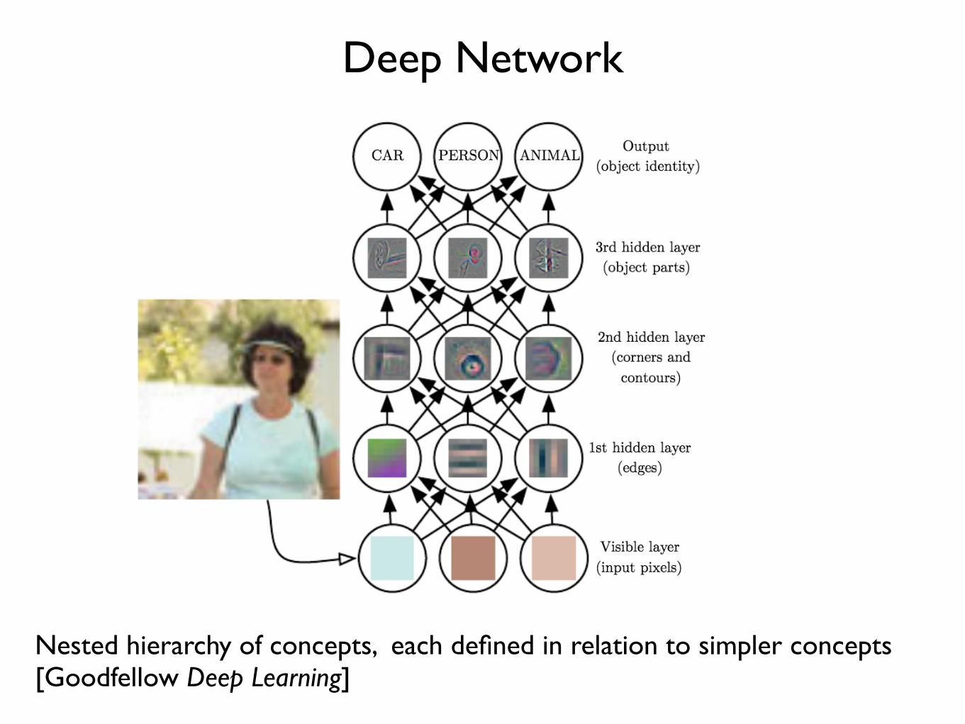
Deep Network
Nested hierarchy of concepts, each defined in relation to simpler concepts [Goodfellow Deep Learning]
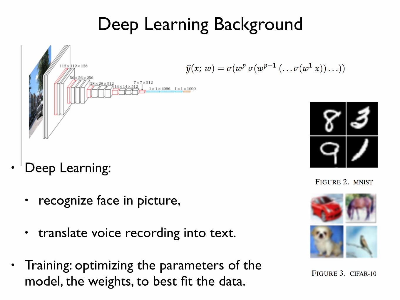
Deep Learning Background
• Deep Learning:
• recognize face in picture,
• translate voice recording into text.
• Training: optimizing the parameters of the model, the weights, to best fit the data.
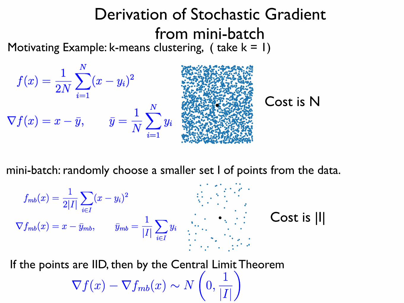
Derivation of Stochastic Gradient from mini-batch
Motivating Example: k-means clustering, ( take k = 1)
If the points are IID, then by the Central Limit Theorem
mini-batch: randomly choose a smaller set I of points from the data.
Cost is N
Cost is |I|
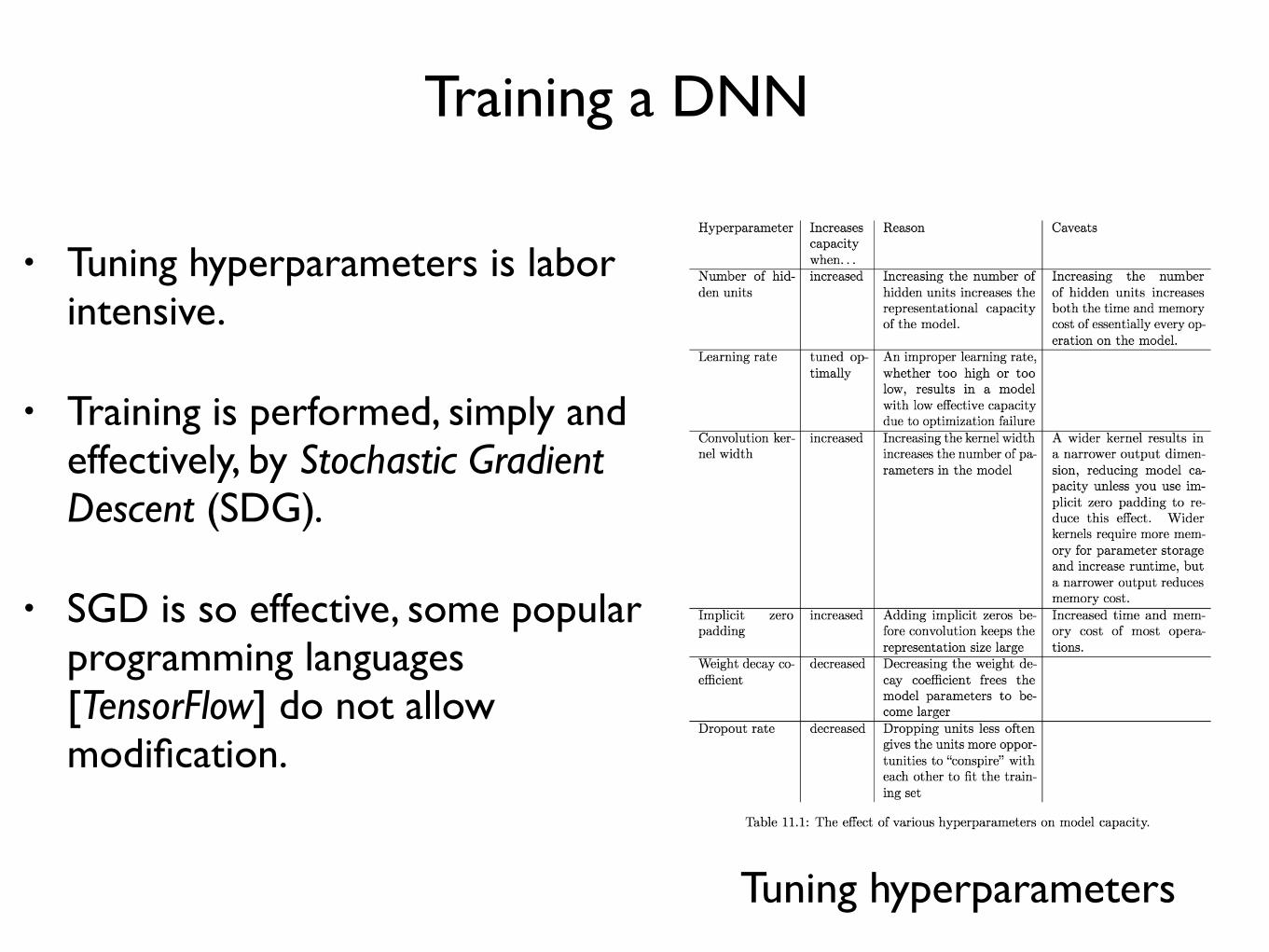
Training a DNN
• Tuning hyperparameters is labor intensive.
• Training is performed, simply and effectively, by Stochastic Gradient Descent (SDG).
• SGD is so effective, some popular programming languages [TensorFlow] do not allow modification.
Tuning hyperparameters

Local Entropy:from Spin Glassesto Deep Networks
to Hamilton-Jacobi PDEs
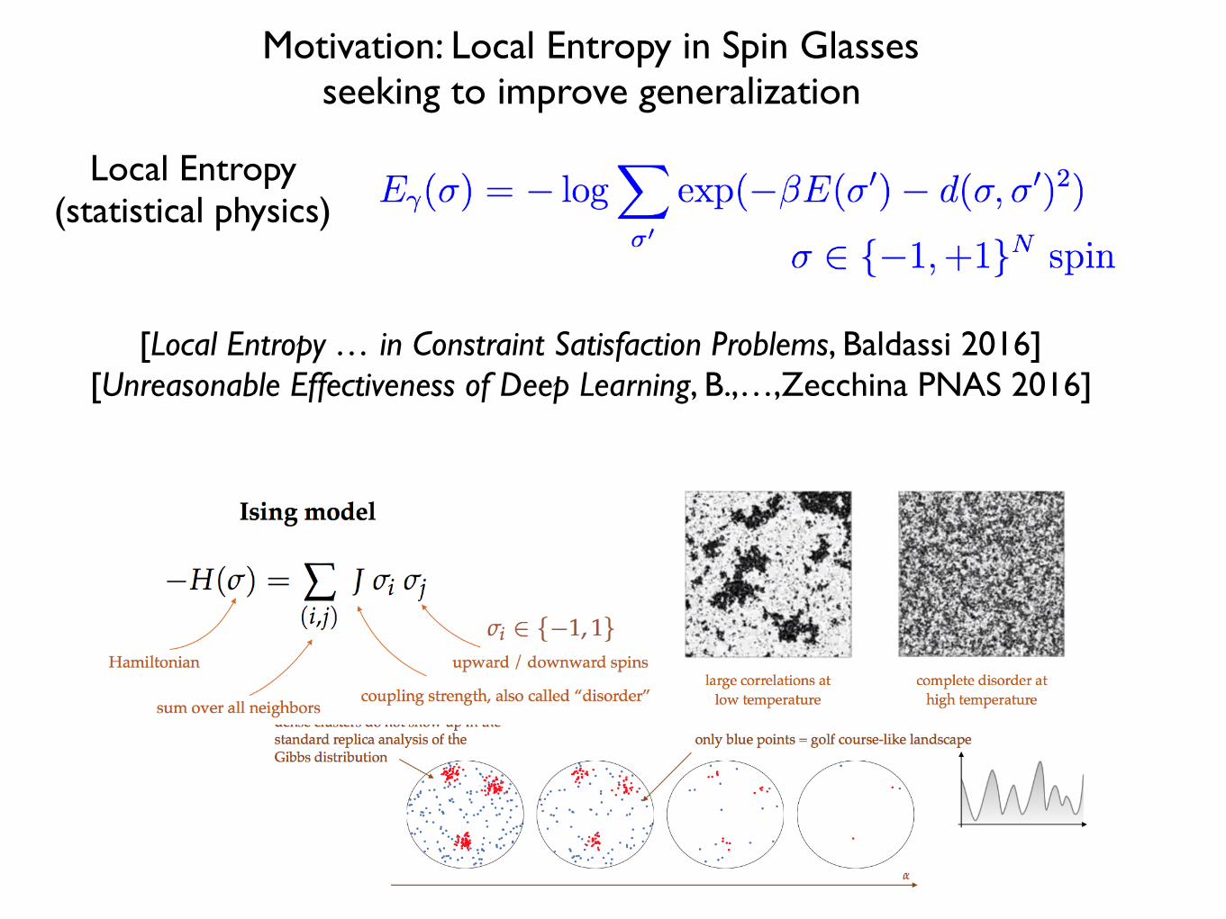
Motivation: Local Entropy in Spin Glassesseeking to improve generalization
Local Entropy (statistical physics)
[Local Entropy … in Constraint Satisfaction Problems, Baldassi 2016][Unreasonable Effectiveness of Deep Learning, B.,…,Zecchina PNAS 2016]
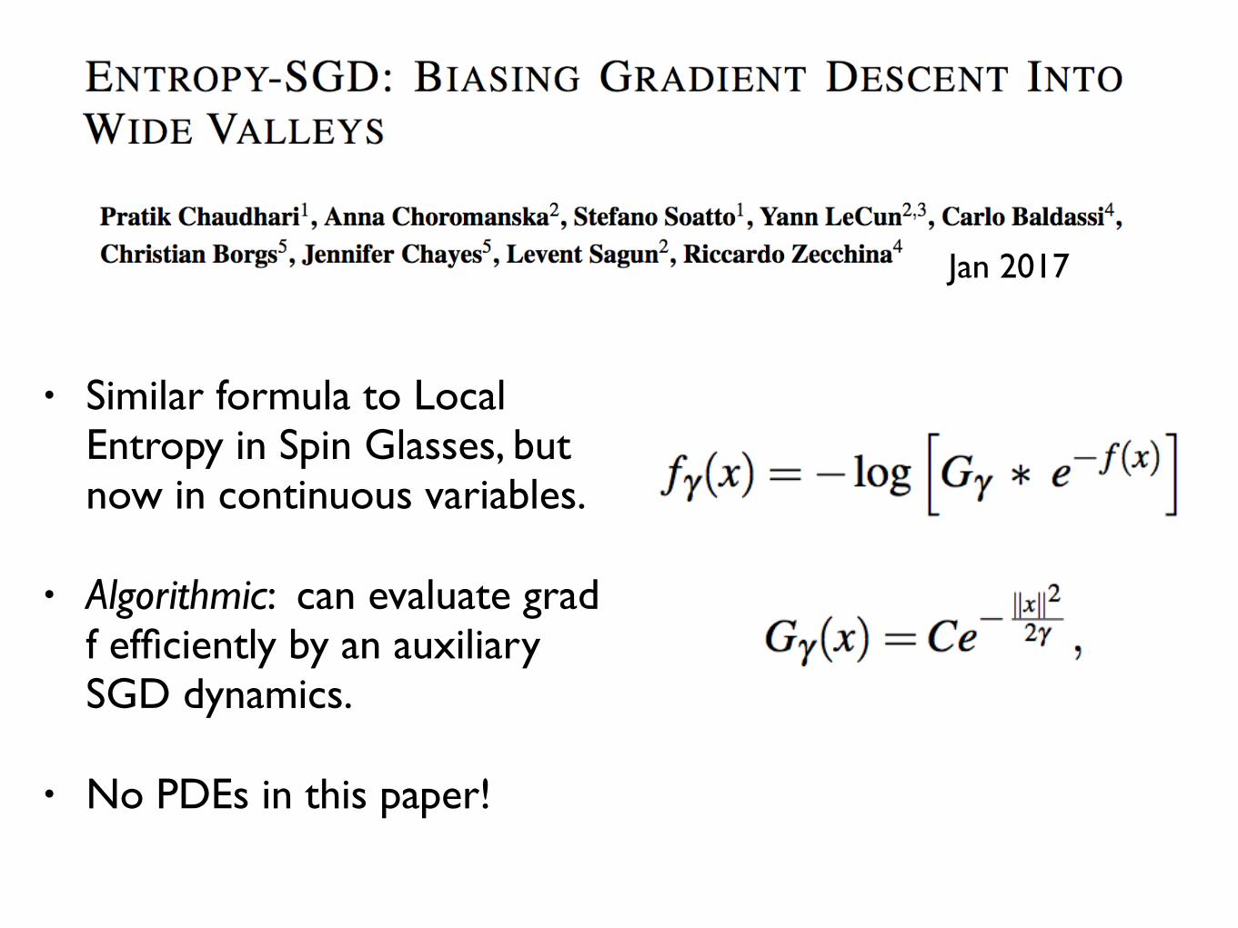
• Similar formula to Local Entropy in Spin Glasses, but now in continuous variables.
• Algorithmic: can evaluate grad f efficiently by an auxiliary SGD dynamics.
• No PDEs in this paper!
Jan 2017
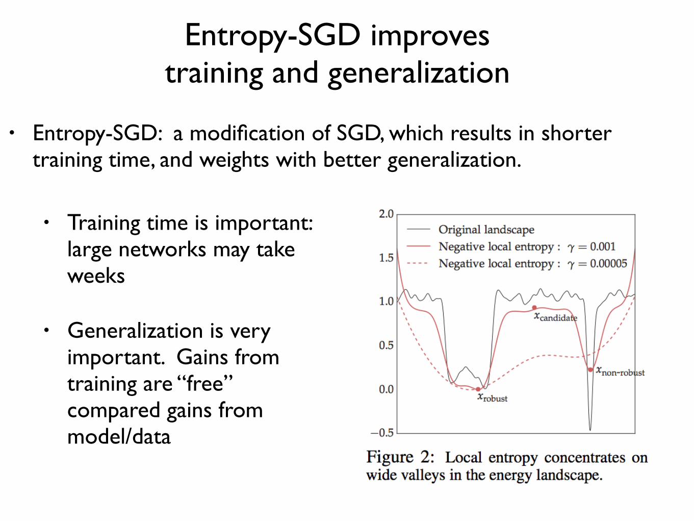
Entropy-SGD improves training and generalization
• Entropy-SGD: a modification of SGD, which results in shorter training time, and weights with better generalization.
• Training time is important: large networks may take weeks
• Generalization is very important. Gains from training are “free” compared gains from model/data
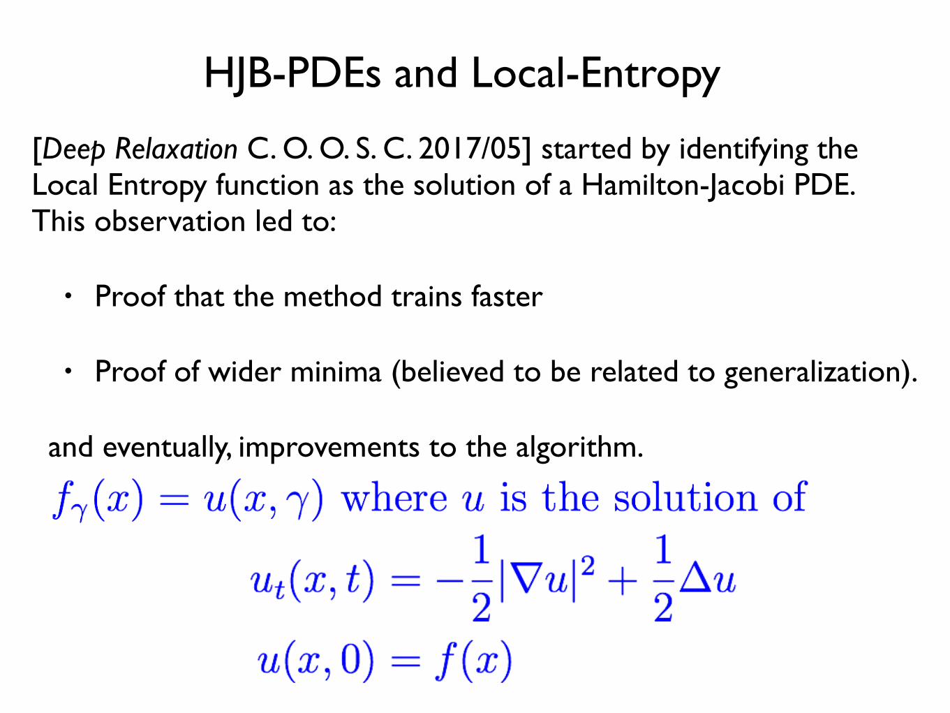
HJB-PDEs and Local-Entropy
[Deep Relaxation C. O. O. S. C. 2017/05] started by identifying the Local Entropy function as the solution of a Hamilton-Jacobi PDE. This observation led to:
• Proof that the method trains faster
• Proof of wider minima (believed to be related to generalization).
and eventually, improvements to the algorithm.

Parallel SGD
EASGD [LeCun … Elastic Averaging SGD] effective parallel training
Very recently new algorithm, PARLE [Chaudry 2017/07], giving best results to date on CIFAR-10, CIFAR-100, SVHN
• ESGD on each processor
• Elastic forcing term between each particle.
• JKO gradient flow interpretation for PARLE:

PDE interpretation of local entropyand equation for the gradient
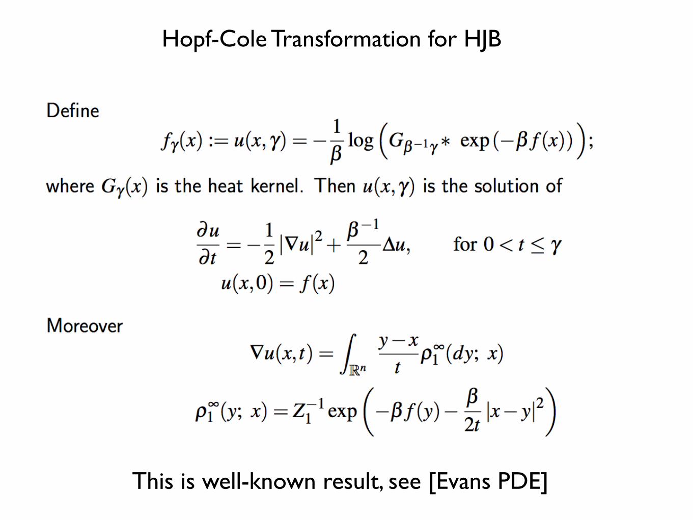
Hopf-Cole Transformation for HJB
This is well-known result, see [Evans PDE]
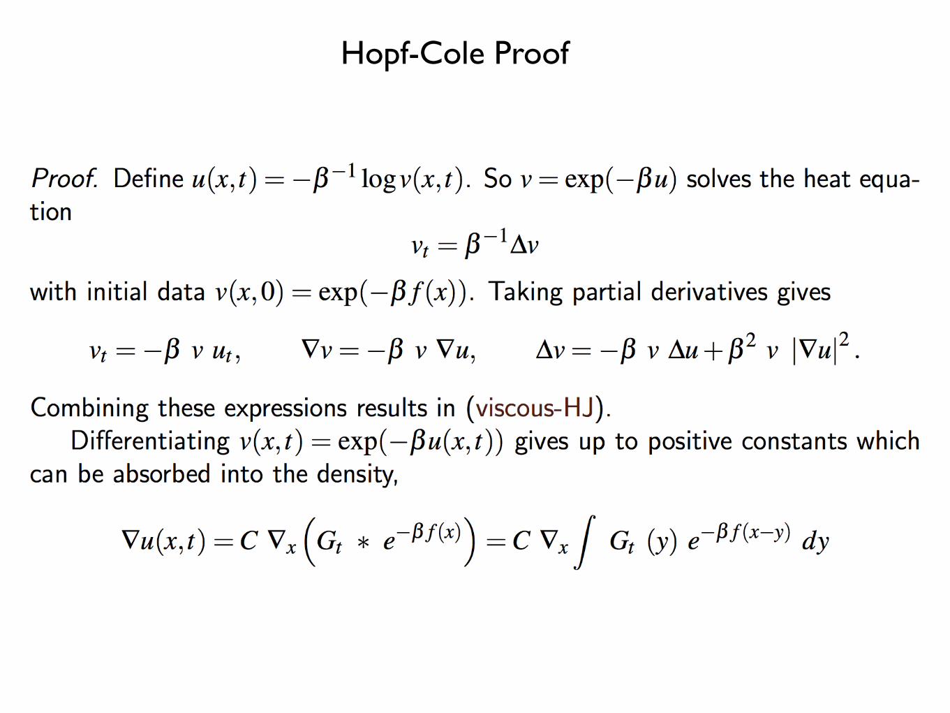
Hopf-Cole Proof
Local Entropy:Visualization
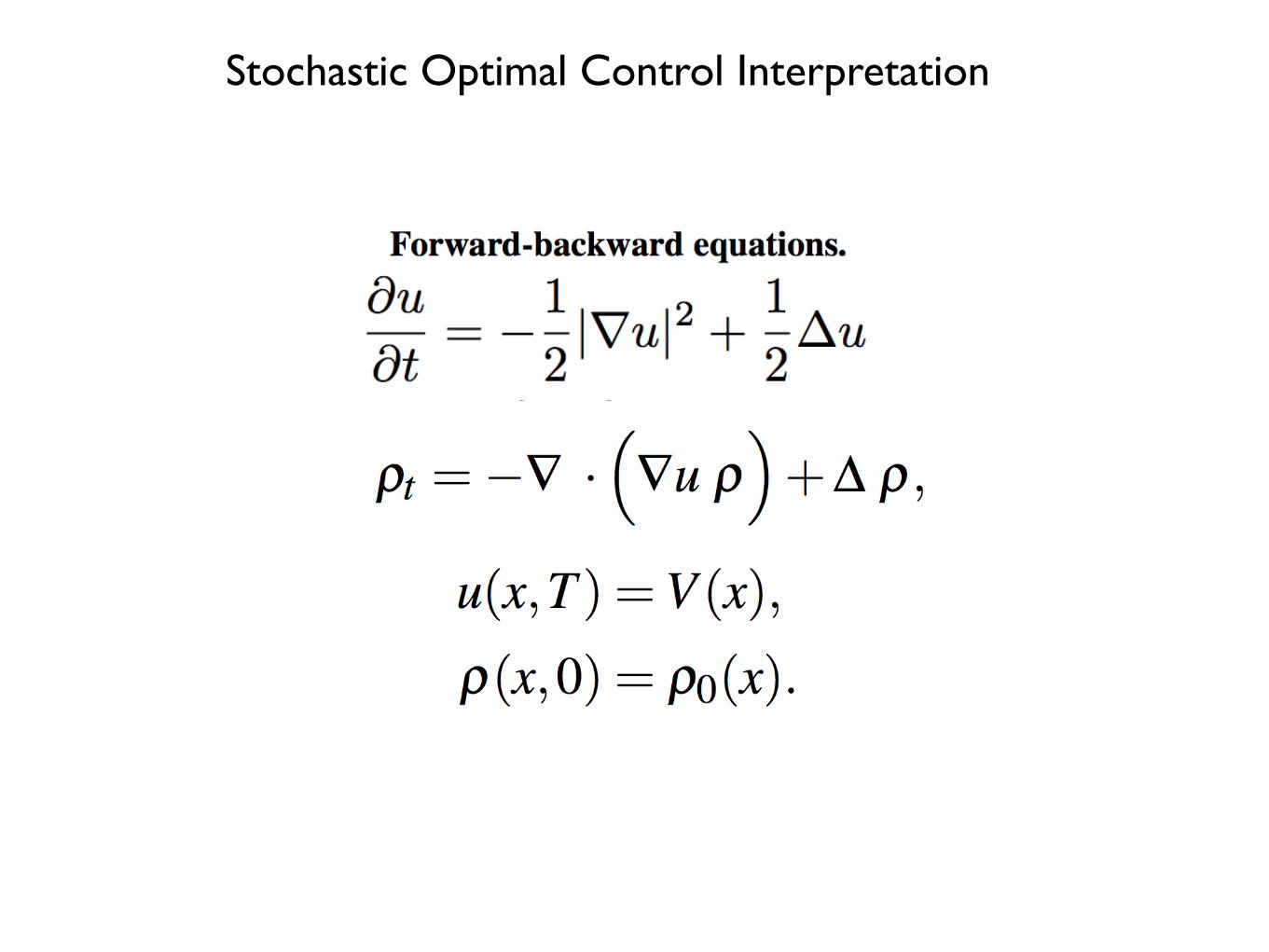
Stochastic Optimal Control Interpretation
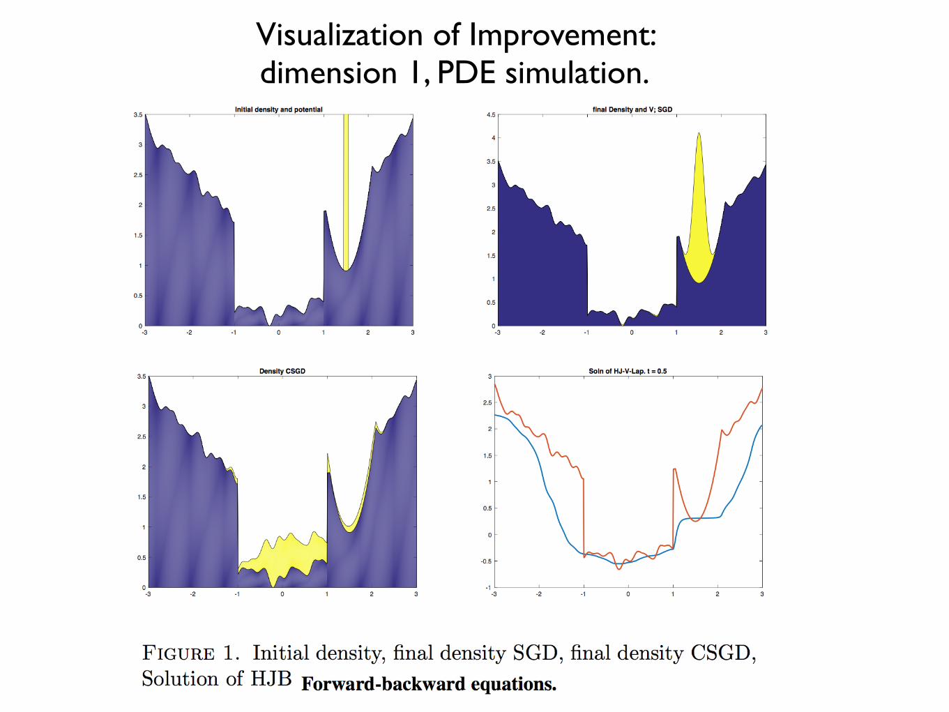
Visualization of Improvement: dimension 1, PDE simulation.

Local Entropy is Regularization using Viscous Hamilton-Jacobi PDE
• True solution in one dimension. (Cartoon in high dimensions, because algorithm only works for shorter times.)
Proof of Improvementfor Modified dynamics
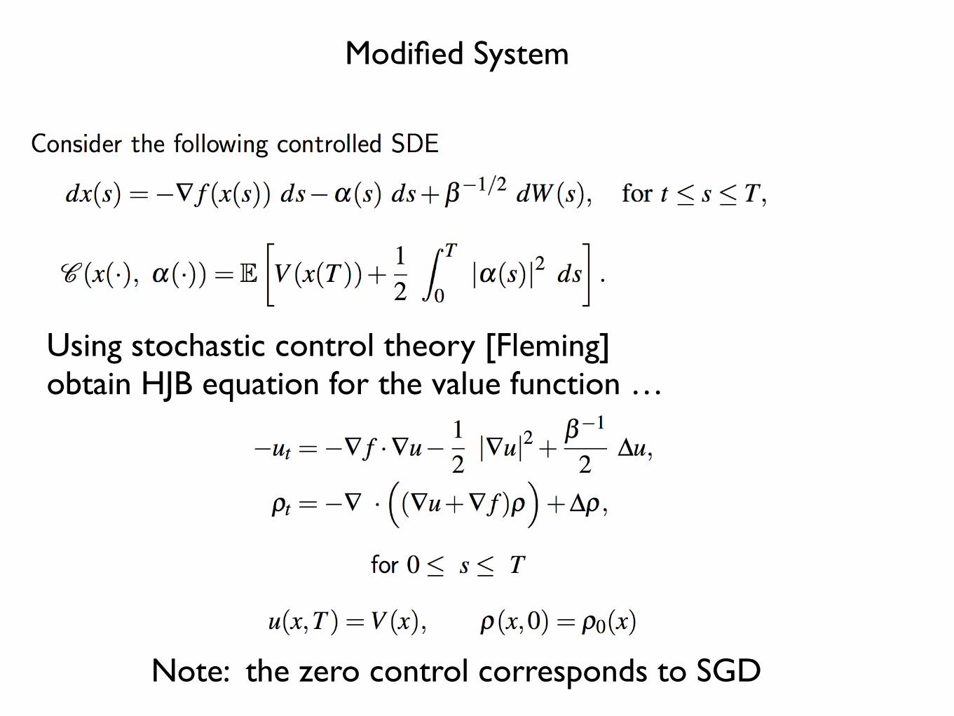
Modified System
Note: the zero control corresponds to SGD
Using stochastic control theory [Fleming] obtain HJB equation for the value function …
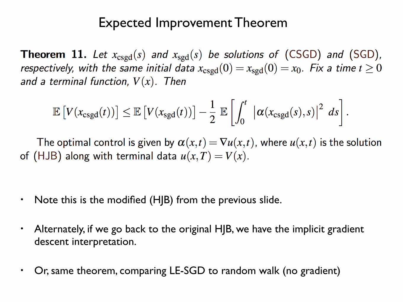
Expected Improvement Theorem
• Note this is the modified (HJB) from the previous slide.
• Alternately, if we go back to the original HJB, we have the implicit gradient descent interpretation.
• Or, same theorem, comparing LE-SGD to random walk (no gradient)
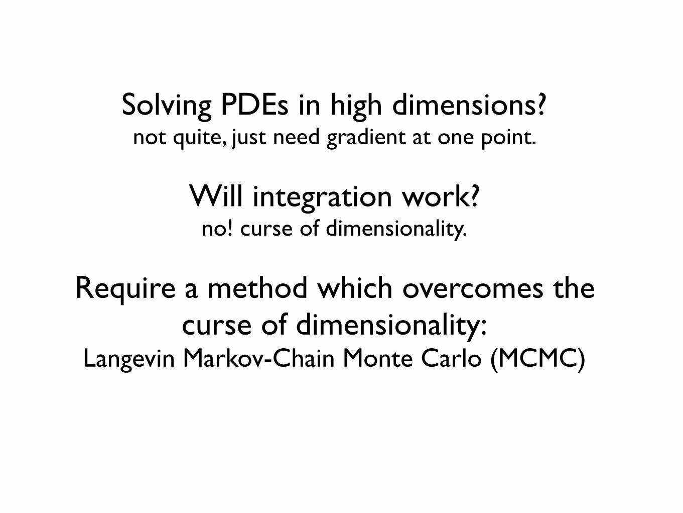
Solving PDEs in high dimensions?not quite, just need gradient at one point.
Will integration work?no! curse of dimensionality.
Require a method which overcomes the curse of dimensionality:
Langevin Markov-Chain Monte Carlo (MCMC)
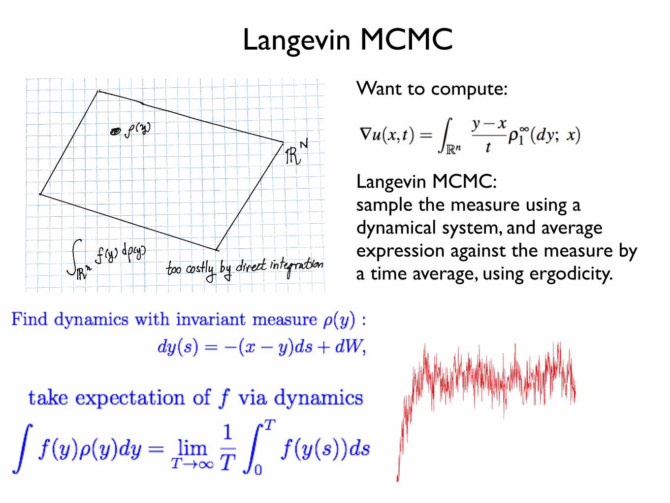
Langevin MCMC
Langevin MCMC: sample the measure using a dynamical system, and average expression against the measure by a time average, using ergodicity.
Want to compute:
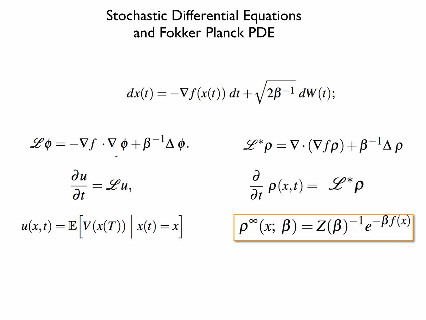
Stochastic Differential Equationsand Fokker Planck PDE

Background: Homogenization of SDEs
• Two scale dynamics
• Unique invariant measure of the fast dynamics
• In the limit, obtain homogenized dynamics
• given by averaging against the invariant measure
• Equivalent by ergodicity to a time average.
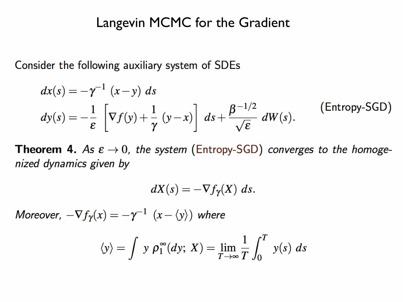
Langevin MCMC for the Gradient

Proof of MCMC for the Gradient
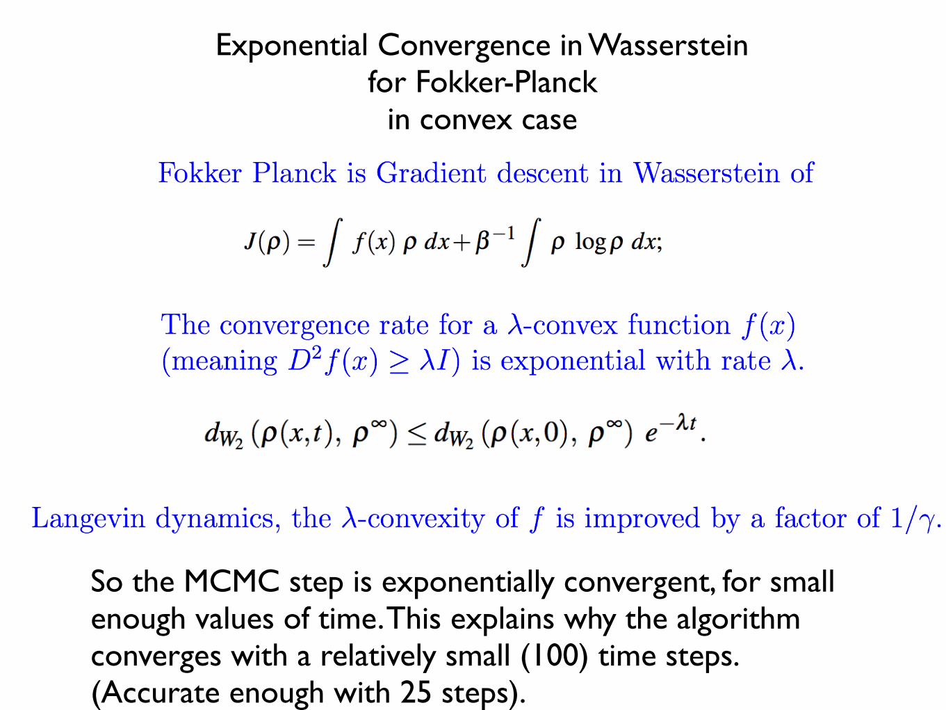
Exponential Convergence in Wasserstein for Fokker-Planck
in convex case
So the MCMC step is exponentially convergent, for small enough values of time. This explains why the algorithm converges with a relatively small (100) time steps. (Accurate enough with 25 steps).

Algorithm and Results in Deep Networks
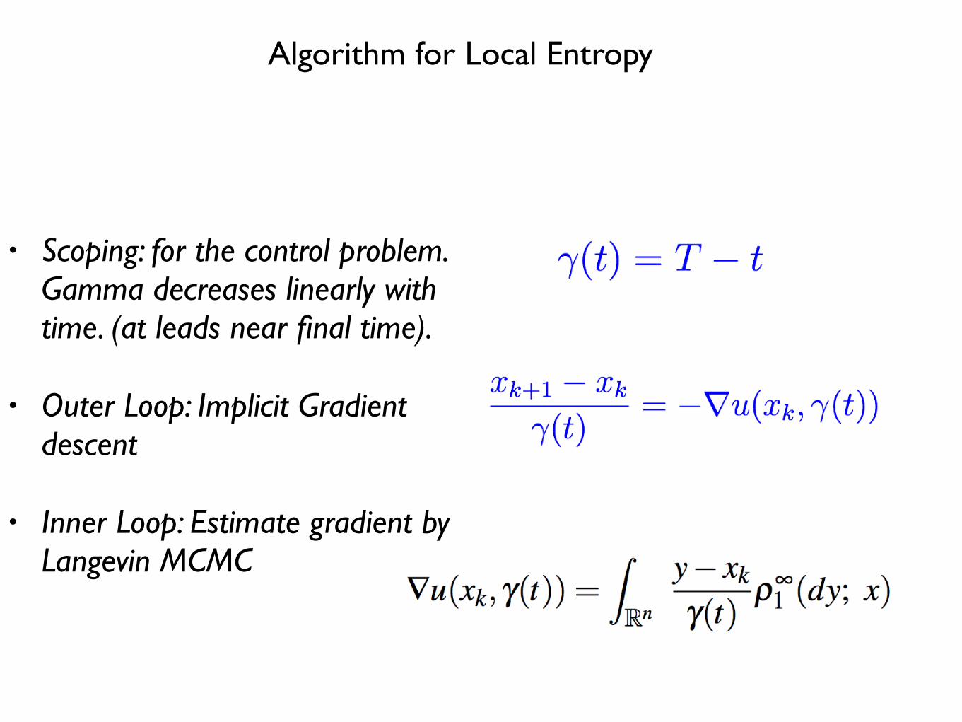
Algorithm for Local Entropy
• Scoping: for the control problem. Gamma decreases linearly with time. (at leads near final time).
• Outer Loop: Implicit Gradient descent
• Inner Loop: Estimate gradient by Langevin MCMC

Numerical Results
Visualization of Improvement in training loss (left)Improve in Validation Error (right)
dimension = 1.67 million
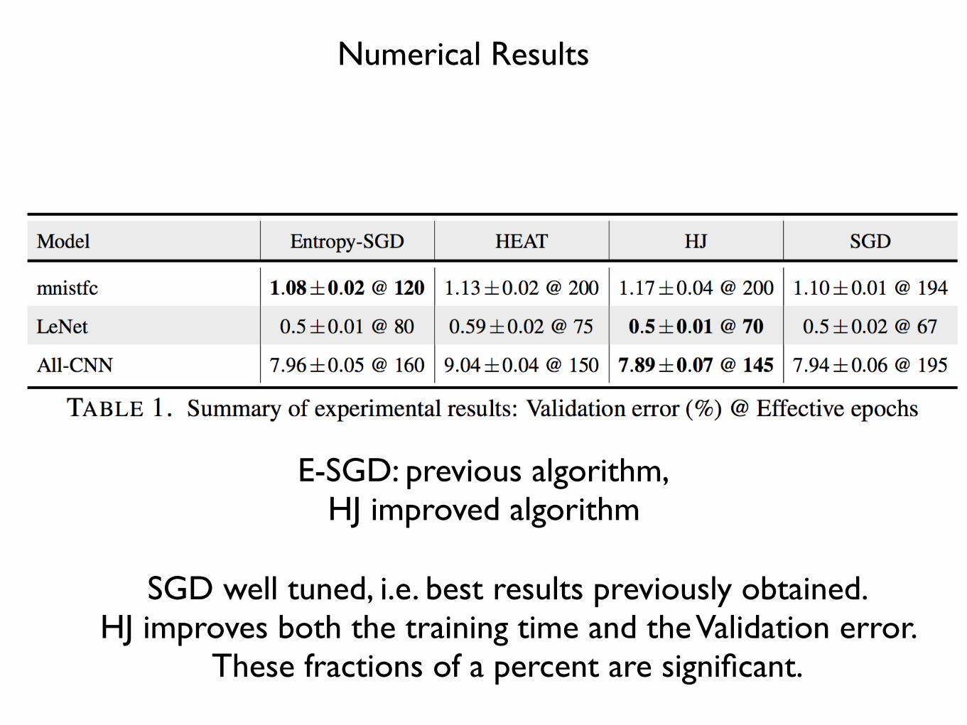
Numerical Results
E-SGD: previous algorithm,HJ improved algorithm
SGD well tuned, i.e. best results previously obtained.HJ improves both the training time and the Validation error.
These fractions of a percent are significant.
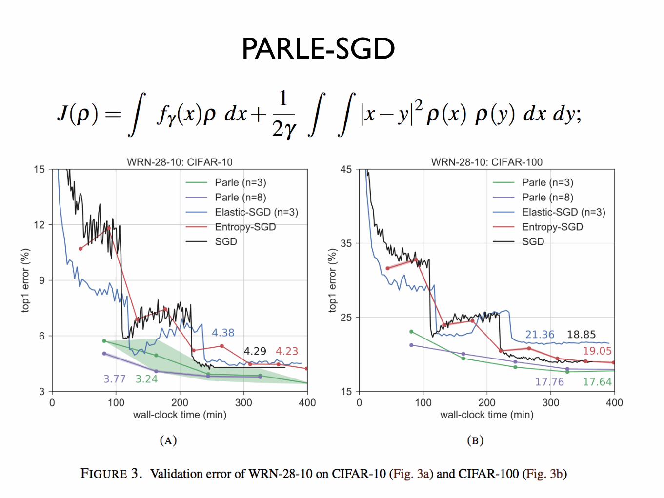
PARLE-SGD
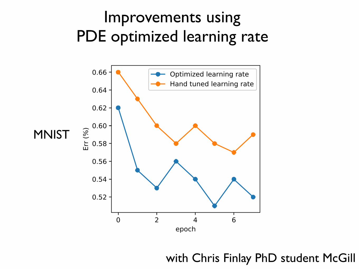
Improvements using PDE optimized learning rate
MNIST
with Chris Finlay PhD student McGill
Optimization:Acceleration methods
Deterministic and Stochastic
HJB gradient as implicit gradient descent
(Most of our analysis is for continuous time in practice, take discrete time steps)

Accelerated Gradient Methods for (non-strictly) convex functions
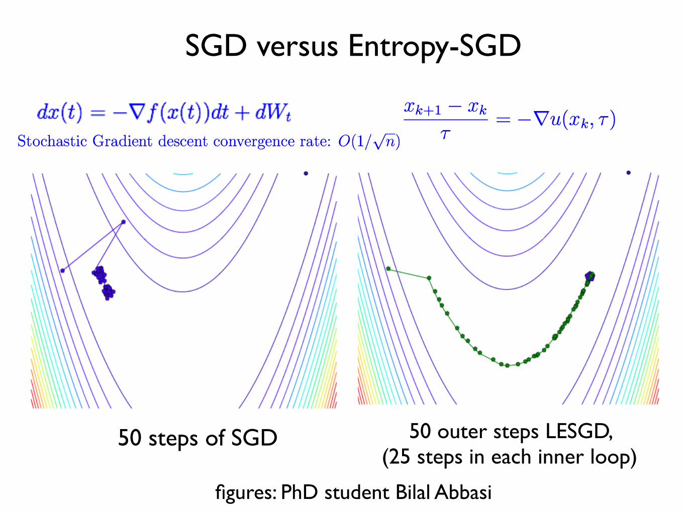
SGD versus Entropy-SGD
figures: PhD student Bilal Abbasi
50 steps of SGD 50 outer steps LESGD, (25 steps in each inner loop)
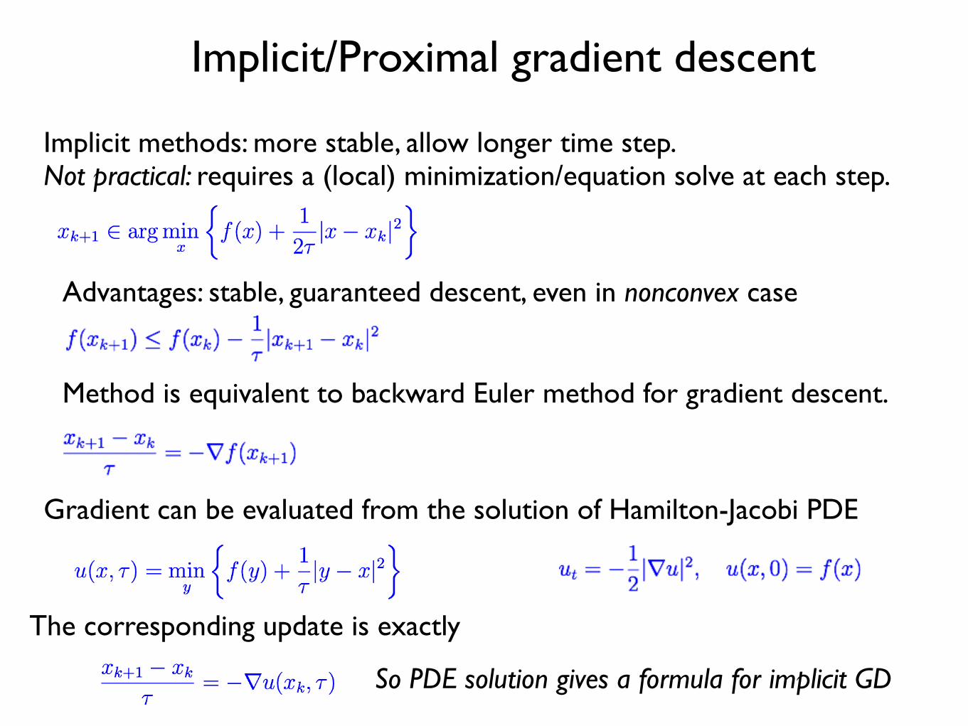
Implicit/Proximal gradient descent
Implicit methods: more stable, allow longer time step.Not practical: requires a (local) minimization/equation solve at each step.
Advantages: stable, guaranteed descent, even in nonconvex case
Method is equivalent to backward Euler method for gradient descent.
Gradient can be evaluated from the solution of Hamilton-Jacobi PDE
The corresponding update is exactly
So PDE solution gives a formula for implicit GD
Fokker-Planck with nonconvex PotentialsChallenges, and insights from
Computational Molecular Dynamics
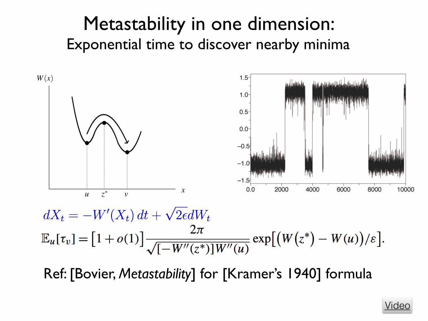
Metastability in one dimension: Exponential time to discover nearby minima
Video
Ref: [Bovier, Metastability] for [Kramer’s 1940] formula
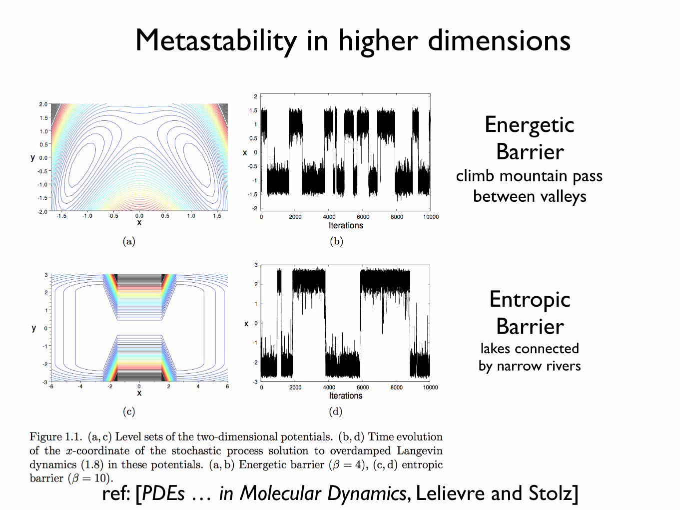
Metastability in higher dimensions
Energetic Barrier
climb mountain pass between valleys
Entropic Barrier
lakes connected by narrow rivers
ref: [PDEs … in Molecular Dynamics, Lelievre and Stolz]
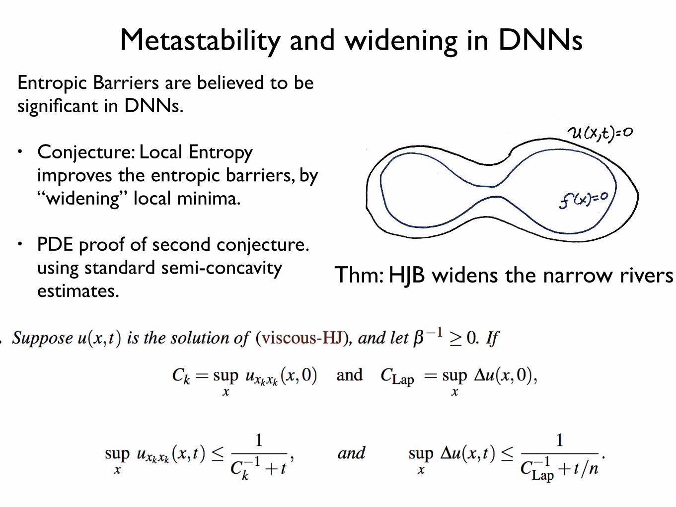
Metastability and widening in DNNsEntropic Barriers are believed to be significant in DNNs.
• Conjecture: Local Entropy improves the entropic barriers, by “widening” local minima.
• PDE proof of second conjecture. using standard semi-concavity estimates.
Thm: HJB widens the narrow rivers
Algorithm Test: K-Means
work in progress with: S. Osher, Mihn Pham, Penghang Yin, UCLA

Algorithm Applied to k-means clustering
• Standard algorithm, Lloyd’s/EM can get stuck in a local minimum.
• Our algorithm, in comparable test case, finds global minimum
• Example on Right: • 4 means, 3 clusters • Optimal solution puts two
means in the double cluster.
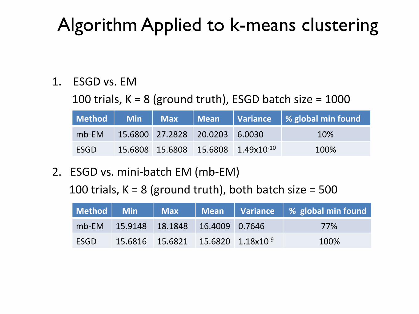
Algorithm Applied to k-means clustering
1.ESGDvs.EM100trials,K=8(groundtruth),ESGDbatchsize=10002.ESGDvs.mini-batchEM(mb-EM)100trials,K=8(groundtruth),bothbatchsize=500
Method� Min� Max � Mean� Variance � %globalminfound�
mb-EM � 15.6800� 27.2828� 20.0203� 6.0030� 10%�
ESGD� 15.6808� 15.6808� 15.6808� 1.49x10⁻¹⁰� 100%�
�
Method� Min� Max � Mean� Variance � %globalminfound�
mb-EM � 15.9148� 18.1848� 16.4009� 0.7646� 77%�
ESGD� 15.6816� 15.6821� 15.6820� 1.18x10⁻⁹� 100%�
• Discovered a HJB-PDE connection with Entropy-SGD algorithm, which has very good performance in Deep Networks.
• Exploited this connection to better understand the algorithm, giving proofs to empirical results about training.
• Improvements to algorithm using PDE insights and numerical PDE ideas.
Conclusions