Q U A N T I T A T I V E R E S E A R C H

Deep Hedging: from Theory to Practice From Greeks to Hedging under Market Frictions

Imperial Frontiers in Quantitative Finance April 24th, 2019 Dr. Hans Buehler * Global Head Equities Analytics, Automation and Optimization & Investor Services QR

Baranidharan Mohan * EMEA Analytics QR

Dr. Ben Wood * EMEA Head Equities Modelling QR

Joint research project with Josef Teichmann ETH Zurich

* Opinions expressed in this paper are those of the authors, and do not necessarily reflect the view of JP Morgan.

Q U

A N

T I

T A

T I

V E

R E

S E

A R

C H

2

Disclaimer

This material is not the product of J.P. Morgan’s Research Department. It is not a research report and is not intended as such. This material is provided for informational purposes only and is subject to change without notice. It is not intended as research, a recommendation, advice, offer or solicitation to buy or sell any financial product or service, or to be used in any way for evaluating the merits of participating in any transaction. Please consult your own advisors regarding legal, tax, accounting or any other aspects including suitability implications for your particular circumstances. J.P. Morgan disclaims any responsibility or liability whatsoever for the quality, accuracy or completeness of the information herein, and for any reliance on, or use of this material in any way. This material is provided on a confidential basis and may not be reproduced, redistributed or transmitted, in whole or in part, without the prior written consent of J.P. Morgan. Any unauthorized use is strictly prohibited. The products and/or services mentioned herein may not be suitable for your particular circumstances and may not be available in all jurisdictions or to all clients. Clients should contact their salespersons at, and execute transactions through, a J.P. Morgan entity appropriately licensed in the client’s home jurisdiction unless governing law permits otherwise. This material is a “solicitation” of derivatives business only as that term is used within CFTC Rule 1.71 and 23.605. Where this material is an “investment recommendation” as that term is defined in MAR visit: www.jpmm.com/#mardisclosures. This material is subject to terms at: www.jpmorgan.com/salesandtradingdisclaimer. © 2019 JPMorgan Chase & Co. All rights reserved. J.P. Morgan is a marketing name for investment banking businesses of J.P. Morgan Chase & Co. and its subsidiaries and affiliates worldwide. Bank products and services, including certain lending, derivative and other commercial banking activities, are offered by JPMorgan Chase Bank N.A. (JPMCB), including through its authorized branches and other global affiliates registered with local authorities as appropriate. Securities products and services, including execution services, are offered in the United States by J.P. Morgan Securities LLC (JPMS LLC), in EMEA by J.P. Morgan Securities plc (JPMS plc) where permitted and in other jurisdictions worldwide by other appropriately licensed global affiliates. JPMCB, JPMS LLC and JPMS plc are principal subsidiaries of JPMorgan Chase & Co. For information on which legal entities offer investment banking products and services in each jurisdiction, please consult: www.jpmorgan.com/ib-legal-entities. For important disclosures in respect of securities transactions, please consult: www.jpmorgan.com/securities-transactions and in respect of over-the-counter equity derivatives transactions, please consult: www.jpmorgan.com/otc-equity-derivative-transactions. For additional regulatory disclosures, please consult: www.jpmorgan.com/disclosures.

Q U

A N

T I

T A

T I

V E

R E

S E

A R

C H

3

Deep Hedging

Summary

– Greek Hedging is a legacy approach once justified by lack of data and computational power

– Statistical Hedging brings data-driven risk management but still relies on classic models for pricing

– Deep Hedging defines a new data-driven “AI” reinforcement learning risk and pricing concept for derivatives. Its challenges are

Realistic and robust simulation of markets

Efficient modern Reinforcement Learning techniques for rapid evolution

Q U

A N

T I

T A

T I

V E

R E

S E

A R

C H

4

Framework

Portfolio

– We are given an portfolio Z of securities and derivatives, all of which are assumed to expire before some terminal maturity T. Negative values represent losses.

We assume interest rates are deterministic, hence we may consider discounted variables.

We assume that FX transactions are cost-free, hence we may assume w.l.g. that all assets are denominated in the same currency.

The portfolio and all subsequent instruments are considered as ``total return” assets. The total return of Z, i.e. the sum of all cash flows of Z at T is denoted by ZT.

– We set T=tm>0 and denote by 0=t0<…<tm-1<T possible intermediate hedging days.

Q U

A N

T I

T A

T I

V E

R E

S E

A R

C H

5

Framework

Mark-to-Model

– At each t we observe relevant market data such as spots, implied vols, rates, etc. We denote this set of market data by X=(X1,…,XK).

– We assume that for each element of our portfolio we have a way to compute a “mark-to-model” value from X.

Volume-weighted mid-prices for equity, FX

Classic derivative pricing models such as Stochastic-Local Vol for derivatives.

– Combined, this yields a (mark-to-) model value Zt for our portfolio.

This is not a tradable quantity.

This meta model will yield a range of classic Greeks in the form of first or higher order derivatives.

Quant Finance as an Interpolation Problem

– Classic derivative models are neither equivalent to the statistical measure Q, nor have they been designed to behave realistically. Their primary objective is interpolation between observable market data in X. A “good” model is measured by:

Quality of fit to reference market data in X, e.g. implied volatilities.

Speed of calibration and execution

Stylized dynamics such as stochastic volatility or stochastic interest rates.

Q U

A N

T I

T A

T I

V E

R E

S E

A R

C H

6

Framework

Hedging – We are given a range of liquid hedging instruments H=H1,…,Hn such as

options, swaps, futures, ETFs, stocks, FX etc. – The mid-price at time t is denoted by Ht, which is a model value

computed from Xt, for example the volume-weighted mid-price for an equity. It is not a tradable quantity.

– The actual price for trading a=(a1,…an) is given by Ht(a):=a Ht + ct(a) in terms of a non-negative and normalized cost function ct. We usually assume ct is convex, but there are valid examples it is not, e.g. fixed fees per trade. Cost can depend on past trading activity to model impact.

Research topic: consistent impact model for option prices. – The formal mark-to-model P&L over the period dt due to trading a in t is

given as a dHt - ct(a) .

We note that this does not take into account unwind cost.

Q U

A N

T I

T A

T I

V E

R E

S E

A R

C H

7

Framework

Liquidity

– Not all instruments are tradable at all times:

An exchange traded option ( Sr – k St )+ for r>t may only be traded at times

u[t,r), i.e. when Si is known and therefore the strike is fixed.

– We denote by At the convex, non-empty set of admissible actions at time t.

The set At may depend all observable market data and our historic trading decisions. For example,

– Short-sell restrictions

– Available liquidity as a function of past trading activity

– Risk limits for our overall position (e.g. maximum Vega exposure)

We call p=(a0,…,am-1) with atAt a trading policy; we will usually omit the “At“ unless necessarily.

dt := a0+…+at-1 is our current position in H.

At time t our mark-to-market is 𝑀𝑡 ≔ 𝑍𝑡 + 𝜹𝑡𝑯𝑡.

The End of the Greek Era

Q U

A N

T I

T A

T I

V E

R E

S E

A R

C H

9

The End of the Greek Era

From Greeks to Statistical Hedging

– Before we focus on Deep Hedging, we discuss alternative approaches.

– Each of these will hedge only over a given period dt.

Q U

A N

T I

T A

T I

V E

R E

S E

A R

C H

10

The Greek Era

Risk-Neutral Hedging

– We denote by 𝜹$ ≔ (𝑋1 ∙ 𝜕𝑋1,…, 𝑋𝐾 ∙ 𝜕𝑋𝐾) the first order “Cash Delta” derivative operator to relevant observable market parameters. We denote by G$ the respective second order “cash Gamma” derivatives and by Q “Theta”.

– The risk-neutral paradigm stipulates to reduce all Delta exposure to zero, i.e. to minimize regardless of cost in each t

sup𝒂𝑡

: − 𝜹$𝑀𝑡 +𝒂𝑡𝜹$𝑯𝑡 ( 𝑀𝑡≔ 𝑍𝑡 + Δ𝑡𝑯𝑡 )

NB: for the L2 norm this can be solved using the Pseudo-inverse of 𝜹$𝑯𝑡.

– This formulation does not take into account trading cost. Ad-hoc heuristics

sup𝒂𝑡

: − 𝜆 𝜹$𝑀𝑡 + 𝒂𝑡𝜹$𝑯𝑡 2

− 𝑐𝑡 𝑎𝑡

Pros – Fast – Needs only today’s market data.

Cons – Inconsistent:

No sense of carry Difficult to add cost to this approach as the “Cash Deltas” have only nominally a $

interpretation: how do we know whether spending 100k$ to hedge a nominal 1m$ vega position is worth it?

– Unrealistic: does not account for “Skew Delta”.

Q U

A N

T I

T A

T I

V E

R E

S E

A R

C H

11

The Greek Era

Parameter Hedging

– We assume that we are estimating a simple normal model 𝑑𝑿𝑡

𝑿𝑡= 𝝁𝑡(𝑿𝑡)𝑑𝑡 + 𝚺𝑡(𝑿𝑡)𝑑𝑾𝑡

for our market parameters, e.g. simply by replaying historic data. This model gives rise to the operator

𝑑(∙) = Δ$𝚺𝑡𝑑𝑾𝑡 + Δ$𝝁𝑡 +1

2𝚺𝑡Γ

$𝚺𝑡 + Θ 𝑑𝑡

– Applying Markoviz’ mean-variance approach to 𝑀𝑡 ≔ 𝑍𝑡 + Δ𝑡𝑯𝑡 yields the intuitive “carry” expression

sup𝒂𝑡

: 𝒂𝑡Δ$𝝁𝑡 +

1

2(𝒂𝑡𝚺𝑡)′Γ

$(𝒂𝑡𝚺𝑡) + Θ 𝑑𝑡 −𝜆

2(𝒂𝑡Δ

$𝚺𝑡)′(𝒂𝑡Δ$𝚺𝑡)𝑑𝑡 − 𝑐𝑡(𝒂𝑡)

Carry term combined

both of Gamma-Theta carry and drift

Risk term driven by the covariance

matrix of X

Implementation cost

Q U

A N

T I

T A

T I

V E

R E

S E

A R

C H

12

The Greek Era

Parameter Hedging

sup𝒂𝑡

: 𝒂𝑡𝜹$𝝁𝑡 +

1

2(𝒂𝑡𝚺𝑡)′Γ

$(𝒂𝑡𝚺𝑡) + Θ 𝑑𝑡 −𝜆

2(𝒂𝑡𝜹

$𝚺𝑡)′(𝒂𝑡𝜹$𝚺𝑡)𝑑𝑡 − 𝑐𝑡(𝒂𝑡)

Pros

– Data-driven combination of carry and risk

– Captures well-known effects such as “skew delta”

– Fast

Cons

– Normal Approximation:

Does not capture strong non-linearities such as short-term barriers

I.e. can lead to strictly worse “hedged” portfolios

– Hedges are only locally optimal / what is the optimal horizon dt vs. the absolute cost term

– Still requires mark-to-model values for Greeks and pricing

Carry term combined both of Gamma-Theta

carry and drift

Risk term driven by the covariance

matrix of X

Implementation cost

Q U

A N

T I

T A

T I

V E

R E

S E

A R

C H

13

Beyond Greeks

Statistical Hedging I – quadratic case

– In our previous example, we effectively approximated the return of a derivative over dt as a normal.

– In Statistical Hedging [2013] we proposed replacing this approximation with genuine historic returns of “the same” derivatives.

For each historic day, use a derivative with the then-same moneyness and time-to-maturity, and compute that derivative’s return over then-dt.

– Do not use today’s fixed derivative terms.

– Compute returns of fixed instruments.

– For path-dependent options, keep past states consistent (e.g. past barrier breaches).

This yields genuine historic returns of both Z and H from t to t+dt.

– In practise, we will want to adjust the drift term to take into account views on relevant carry: e.g. just because the S&P went up for the last years does not mean we wish to capture this with our model topic of model uncertainty

Q U

A N

T I

T A

T I

V E

R E

S E

A R

C H

14

Beyond Greeks

Statistical Hedging I – quadratic case

– Given returns dMt and dHt we may now solve the Markoviz problem

sup𝒂𝑡

: E[𝑑𝑀𝑡 + 𝒂𝑡𝑑𝑯𝑡]𝑑𝑡 −𝜆

2Var[𝑑𝑀𝑡 + 𝒂𝑡𝑑𝑯𝑡] − 𝑐𝑡(𝒂𝑡)

– We note that if all variables are well approximated by our previous normal representation, then the two approaches coincide.

Carry term derived from historical

performane

Risk term driven by the covariance

matrix of X

Implementation cost

Q U

A N

T I

T A

T I

V E

R E

S E

A R

C H

15

Beyond Greeks

What is wrong with Markoviz for Derivatives?

__ Risk aversion levels manually calibrated to roughly fit between CVaR and Mean-Dispersion measure: Mean-MAD 1, Mean-Vol 1, CVaR 1.5, Quadratic VaR 0.5.

Mean-Dispersion measures are not monotone

𝑈 𝐴 ≔ E 𝐴 −𝜆

2𝐴 − E[𝐴] 𝑝

… it makes very little sense to optimize

over a non-monotonic objective.

Graph shows the fair risk-adjusted price for taking on a short position in a digital call. The lower the strike, the higher the required compensation.

NB: Mean-Variance, Mean-Volatility, Mean-Square, … all have

the same issue of not being monotone.

Q U

A N

T I

T A

T I

V E

R E

S E

A R

C H

16

Beyond Greeks

What is wrong with Markoviz for Derivatives?

Using entropy vs. mean-variance to hedge a net long butterfly position maturing tomorrow. Data generated with BS model, 50% vol. The same vanillas which compose the butterfly are

available to trade for free.

Increased Risk Aversion

Mean-variance sells a net long position for positive cost to reduce perceived

“variance” risk

Q U

A N

T I

T A

T I

V E

R E

S E

A R

C H

17

Beyond Greeks

Statistical Hedging II – Convex Risk Measures – Mean-Variance is not monotone; we therefore move to a systematic approach to

measure carry/risk: we call U a risk-adjusted return if U is normalized to U(0) = 0. U is monotone, i.e. AB then U(A) U(B). U is concave. U is cash-invariant, U(A+c) = U(A) + c for all constants c.

– We note –U is a convex risk measure.

– A classic example is the entropy risk-adjusted return 𝑈 𝐴 ≔ −1

𝜆log E[exp(−𝜆𝐴)].

Another important example is (the negative of) CVaR. – Boundary cases for most reasonable U’s: E 𝐴 ≥ 𝑈 𝐴 ≥ −inf (𝐴) – We now solve the local problem

sup𝒂𝑡

: U 𝑑𝑀𝑡 + 𝒂𝑡𝑑𝑯𝑡 − 𝑐𝑡 𝒂𝑡

which we may also write in terms of the associated dispersion risk measure 𝜌 𝐴 ≔ −𝑈(𝐴 − 𝐸 𝐴 ) as

sup𝒂𝑡

: E 𝑑𝑀𝑡 + 𝒂𝑡𝑑𝑯𝑡 − 𝜌(𝑑𝑀𝑡 + 𝒂𝑡𝑑𝑯𝑡) − 𝑐𝑡(𝒂𝑡)

This resembles the previous carry-risk-cost representation.

Q U

A N

T I

T A

T I

V E

R E

S E

A R

C H

18

Beyond Greeks

Cost vs. Risk Aversion – Quadratic CVaR Example

Increased Risk Aversion

Increased

Co

st

Super-Hedging under extreme

risk aversion

Hedge only spot

Here we see less hedging vs. cash

injection: trading is more expensive

than injecting more cash

𝑈 𝐴 ≔ −inf𝑤

𝑤 + 1 + 𝜆 𝐴 + 𝑤 −2

Q U

A N

T I

T A

T I

V E

R E

S E

A R

C H

19

Beyond Greeks

Statistical Hedging

sup𝒂𝑡

: U(𝑑𝑀𝑡 + 𝒂𝑡𝑑𝑯𝑡) − 𝑐𝑡(𝒂𝑡)

Pros

– Data-driven combination of carry and risk which captures non-linearities

– Captures well-known effects such as “skew delta”

– Monotone, convex hedged portfolios.

Cons

– Hedges are only locally optimal / what is the optimal horizon dt vs. the absolute cost term

– Still requires mark-to-model values for return computation and pricing

– Compute intensive

Q U

A N

T I

T A

T I

V E

R E

S E

A R

C H

20

The End of the Greek Era

Summary

– Classic Greek Hedging is unsuitable for data-driven risk management

– Parametric Hedging works for very smooth portfolios

– Statistical Hedging expands this to strong non-linear features

Challenges

– Future hedging cost for the now-optimal portfolio are not taken into account: tomorrow’s mark-to-model value is assumed to be realizable.

– Pricing relies on classic model prices, possibly with some ad-hoc adjustment due to immediate hedging cost.

Deep Hedging

– Simulate the market to maturity and then solve the generic problem

sup𝒂0…𝒂𝑇−1

: U 𝑍𝑇 + 𝜹𝑡𝑑𝑯𝑡

𝑇−1

𝑡=0− 𝑐𝑡 𝒂𝑡

𝑇−1

𝑡=0

Deep Hedging

Q U

A N

T I

T A

T I

V E

R E

S E

A R

C H

22

Deep Hedging

Deep Hedging

– Simulate the market to maturity and then solve the generic problem

sup𝒂0…𝒂𝑇−1

: U 𝑍𝑇 + 𝜹𝑡𝑑𝑯𝑡

𝑇−1

𝑡=0− 𝑐𝑡 𝒂𝑡

𝑇−1

𝑡=0

– Classic “hedging under market frictions” problem.

Challenges

– Theory

– Numerical implementation

– Market dynamics

Q U

A N

T I

T A

T I

V E

R E

S E

A R

C H

23

Theory

Deep Hedging

𝑣∗ 𝑍 ≔ sup𝜋=𝒂0…𝒂𝑇−1

: U 𝑍𝑇 + 𝜹𝑡𝑑𝑯𝑡

𝑇−1

𝑡=0− 𝑐𝑡 𝒂𝑡

𝑇−1

𝑡=0

Statistical Arbitrage

– We say the market has statistical arbitrage if 𝑣∗ 0 > 0. This does not imply presence of strict arbitrage.

Example: Black & Scholes model with positive drift. Strictly speaking, presence of strict arbitrage also does not imply presence of

statistical arbitrage. Example: market has 100 scenarios, in 6 of which the asset returns 0%. In all other scenarios the asset returns 1%. Under CVaR@95%, 𝑣∗ 0 = 0.

– Statistical Arbitrage is real – it means there are opportunities in the market, depending on one’s risk aversion. Example: realized-implied vol carry; rates curve carry etc.

– However, it can pollute the question of risk management: just as in classic cash portfolio optimization the estimation of “alpha” is much more involved. We may therefore separate the estimation of carry from the estimation of the

higher moments of the distribution of our instruments. – We call a trade a static arbitrage opportunity if the return is non-negative under

any market dynamics (e.g. violation of butterfly or calendar arb).

Q U

A N

T I

T A

T I

V E

R E

S E

A R

C H

24

Theory

Deep Hedging

𝑣∗ 𝑍 ≔ sup𝜋=𝒂0…𝒂𝑇−1

: U 𝑍𝑇 + 𝜹𝑡𝑑𝑯𝑡

𝑇−1

𝑡=0− 𝑐𝑡 𝒂𝑡

𝑇−1

𝑡=0

Pricing

– Consider a current position of Z. The price of selling a derivative Y to a customer is given by the marginal cost

𝑝(𝑌) ≔ 𝑣∗ 𝑍 − 𝑌 − 𝑣∗ 𝑍

Of course, 𝑣∗ 𝑍 − 𝑌 + 𝑝(𝑌) = 0.

Reflects naturally a bid/ask spread.

The model-price is no longer used.

Q U

A N

T I

T A

T I

V E

R E

S E

A R

C H

25

Theory

Deep Hedging

𝑣∗ 𝑍 ≔ sup𝜋=𝒂0…𝒂𝑇−1

: U 𝑍𝑇 + 𝜹𝑡𝑑𝑯𝑡

𝑇−1

𝑡=0− 𝑐𝑡 𝒂𝑡

𝑇−1

𝑡=0

Hamilton-Jacobi-Bellman

– One of the biggest short comings of the approach presented here is that Z is fixed and not a part of the “state” of the market.

– The Bellman form of the problem can be written as follows:

Denote by Mt all future cash flows of our portfolio on and after t, and by mt the cashflow arising from holding Mt at t. This gives the classic HJB reward form

𝑉∗ 𝑀𝑡|𝑺𝑡 = sup

𝑎𝑡

: 𝑈 𝑉∗ 𝑀𝑡+1 + 𝒂𝑡𝐻𝑡+1 |𝑺𝑡 − 𝑐 𝒂𝑡|𝑺𝑡 +𝑚𝑡

Research topics: – Find a representation for a portfolio of derivatives which is efficient for this to

be applicable.

– Under what conditions does this equation have a fixed point for all combined states (Mt,St).

Q U

A N

T I

T A

T I

V E

R E

S E

A R

C H

26

Theory

Deep Hedging

𝑣∗ 𝑍 ≔ sup𝜋=𝒂0…𝒂𝑇−1

: U 𝑍𝑇 + 𝜹𝑡𝑑𝑯𝑡

𝑇−1

𝑡=0− 𝑐𝑡 𝒂𝑡

𝑇−1

𝑡=0

Pricing

– Consider a current position of Z. The price of selling a derivative Y to a customer is given by the marginal cost

𝑝(𝑌) ≔ 𝑣∗ 𝑍 − 𝑌 − 𝑣∗ 𝑍

Of course, 𝑣∗ 𝑍 − 𝑌 + 𝑝(𝑌) = 0.

Reflects naturally a bid/ask spread.

The model-price is no longer used.

Q U

A N

T I

T A

T I

V E

R E

S E

A R

C H

27

Numerical Implementation

Deep Hedging

sup𝜋=𝒂0…𝒂𝑇−1

: U 𝑍𝑇 + 𝜹𝑡𝑑𝑯𝑡

𝑇−1

𝑡=0− 𝑐𝑡 𝒂𝑡

𝑇−1

𝑡=0

Structure of the Problem

– The problem above is convex in p. – We will solve this over a fixed set of paths, and therefore fixed set of terminal payoffs. – Path-dependency of the problem enters due to transaction cost and from path-dependent

restrictions on liquidity. Reinforcement Learning

– Parameterize at as a neural network, with the result of the previous step feeding into the next step.

– This is called “model-based policy search” in the ML literature. – Theoretical result [DH’18]: neural networks approximate any policy arbitrarily well with

increasing depth and width. – Practical choices:

Each at has its own network rather deep network Share network across t LSTM to capture path

– Example code in Karas is just about a page of code https://people.math.ethz.ch/~jteichma/deep_portfolio_optimization_keras.html

– Efficient, scalable, model-independent implementation.

Q U

A N

T I

T A

T I

V E

R E

S E

A R

C H

28

Numerical Implementation

Deep Hedging

– We show the efficiency and impact of the algorithm for classic derivative model dynamics.

– Used to validate convergence of the numerical scheme against (the few) analytically available results.

– Even here, we are able to compute previously inaccessible problems for entire portfolios of derivatives

Q U

A N

T I

T A

T I

V E

R E

S E

A R

C H

29

Deep Hedging

Comparison with theory: vanilla option with Heston dynamics

– Hedge an ATM 30-day call with spot and var swap

– No costs, no limits, 50% CVaR value function

PnL distribution

Spot hedge

Spot price Var swap price

Q U

A N

T I

T A

T I

V E

R E

S E

A R

C H

30

Deep Hedging

Comparison with theory: Heston dynamics with cost

– We have asymptotic results for small transaction cost for classic one-factor models such as Black Scholes.

– There are no analytic results for higher order models. We show that the same asymptotics hold using our numerical scheme

Black-Scholes for which we know

theoretical results

Heston No theoretical results but

we plot the 1-factor expected behaviour

Q U

A N

T I

T A

T I

V E

R E

S E

A R

C H

31

Deep Hedging

– 30-day ATM call option

– Plot shows spot hedge (“Delta”)

– No limits

– Entropic value

– Risk aversion 10

– Black-Scholes simulator

Vanilla option: impact of transaction costs

Q U

A N

T I

T A

T I

V E

R E

S E

A R

C H

32

Deep Hedging

Forward starting option: impact of transaction costs

Daily Delta Amount from 0th day to Maturity

– 30-day ATM call starting in 15 days

– Heston simulator, no limits, entropic value, risk aversion 50

– Hedge with spot only

Incremental delta

Q U

A N

T I

T A

T I

V E

R E

S E

A R

C H

33

Deep Hedging

Forward starting option: impact of transaction costs

Total Delta Amount from Ref day to Maturity

– 30-day ATM call starting in 15 days

– Heston simulator, no limits, entropic value, risk aversion 50

– Hedge with spot only

Total delta

Q U

A N

T I

T A

T I

V E

R E

S E

A R

C H

34

Deep Hedging

Popular retail payoff:

– Client is short a down-and-in put paid at maturity

– Upper knockout barrier

– Fixed coupons until KO

Market

– 0.1% transaction costs

– No limits

– Risk aversion 20

– Entropic value

– Monthly hedging

– Local volatility simulator

Total delta Incremental delta

Sample paths

Depending on the state (barrier breached) future

delta changes

Q U

A N

T I

T A

T I

V E

R E

S E

A R

C H

35

Deep Hedging

Deep Hedging with Classic Derivatives Generators

– Useful for assessing liquidity and cost impact at scale

Straightforward with TensorFlow

Inherently parallelizable since risk-adjusted returns tend to be expectation based.

Speed independent of number of instruments in portfolio

Asset-class agnostic: discounting, FX, own callability etc all no problem

Client-callability: master thesis under way @ ETH

…. shouldn’t we use the real market to train our model?

Market Dynamics

Q U

A N

T I

T A

T I

V E

R E

S E

A R

C H

37

Market Dynamics

Challenges

– Sparse data set vs. large number of instruments.

– Non-stationarity and robustness Idea: solve a robust version of our problem,

inf𝑄: sup𝜋=𝒂0…𝒂𝑇−1

: U𝑄 𝑍𝑇 + 𝜹𝑡𝑑𝑯𝑡𝑇−1𝑡=0 − 𝑐𝑡 𝒂𝑡

𝑇−1𝑡=0

– Avoid static arbitrage A possible approach is parameterizing the implied vol in “discrete local vol” (see also Wissel) which is an arb-free parameterization.

Model Challenges

– Statistical arbitrage.

Robustify the estimator.

Find the closest risk-neutral measure without drift.

Q U

A N

T I

T A

T I

V E

R E

S E

A R

C H

38

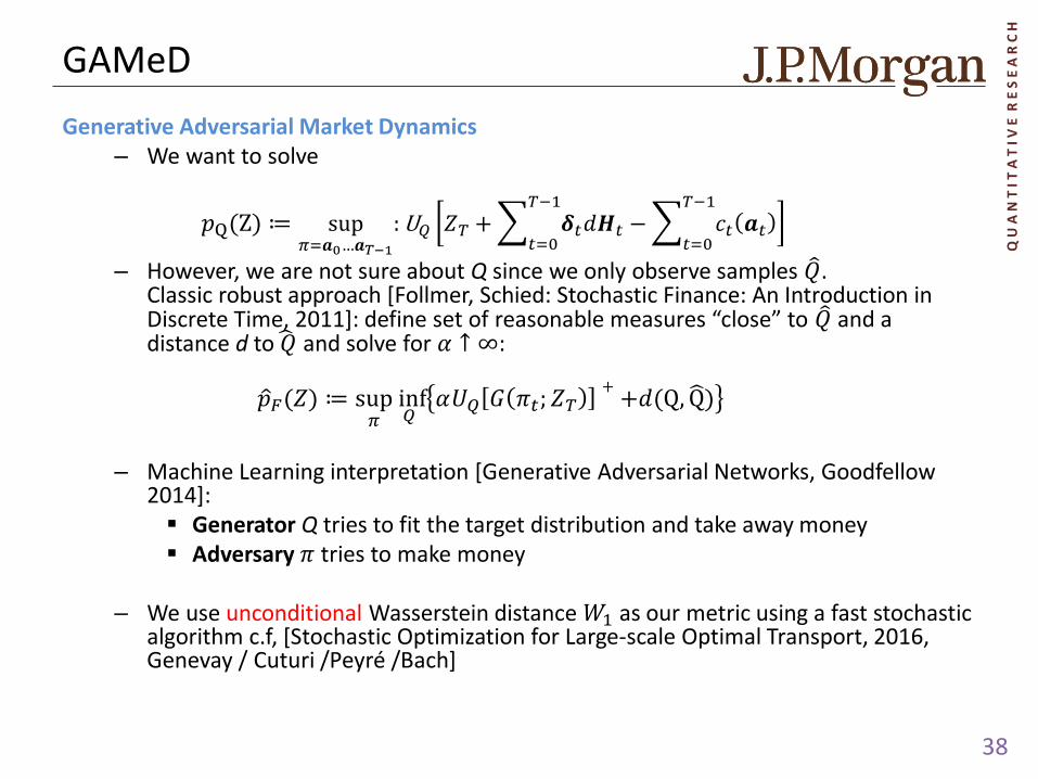
GAMeD

Generative Adversarial Market Dynamics – We want to solve

𝑝Q(Z) ≔ sup𝜋=𝒂0…𝒂𝑇−1

: U𝑄 𝑍𝑇 + 𝜹𝑡𝑑𝑯𝑡

𝑇−1

𝑡=0− 𝑐𝑡 𝒂𝑡

𝑇−1

𝑡=0

– However, we are not sure about Q since we only observe samples 𝑄 . Classic robust approach [Follmer, Schied: Stochastic Finance: An Introduction in Discrete Time, 2011]: define set of reasonable measures “close” to 𝑄 and a distance d to 𝑄 and solve for 𝛼 ↑ ∞:

𝑝 𝐹(𝑍) ≔ sup𝜋 inf𝑄

𝛼𝑈𝑄 𝐺 𝜋𝑡; 𝑍𝑇++𝑑(Q, Q )

– Machine Learning interpretation [Generative Adversarial Networks, Goodfellow

2014]: Generator Q tries to fit the target distribution and take away money Adversary 𝜋 tries to make money

– We use unconditional Wasserstein distance 𝑊1 as our metric using a fast stochastic

algorithm c.f, [Stochastic Optimization for Large-scale Optimal Transport, 2016, Genevay / Cuturi /Peyré /Bach]

Q U

A N

T I

T A

T I

V E

R E

S E

A R

C H

39

GAMeD

STOXX50 Dataset

– We obtain historical spot and option prices for last 10 years of data ~ 2000 historical data points

– Option Grid with relative strikes 𝐾 = {0.8, 0.85, 0.9, 0.95, 1.0, 1.05, 1.1, 1.15, 1.2}, and maturities of 𝑇 = {20, 40, 60, 80, 100, 120} days

– 𝑯𝑡 = 109-dimensional vector = 1 Spot + 54 Calls + 54 Puts

– At every time step, 𝑯𝑡 = generated prices for the grid of options + spot

– Each simulation time step = 20 days to match the maturities

K

T

K

T 𝑯0 𝑯1

K

T 𝑯𝑡

Day 0 Day 20

Q U

A N

T I

T A

T I

V E

R E

S E

A R

C H

40

GAMeD

Setup and Training

– Generator network: 2 layer LSTM of size 64, 𝑓 ~62K parameters

– Hedger network: 2 layer LSTM of size 64, 𝜋 ~112K parameters

– Use 2% transaction costs to regularize the hedger network

– Training:

Train with batch sizes of 32K to minimize noise, RMS Prop with a learning rate of 1e-4

Dropout of 25% between state-to-state LSTM connections to regularize training

50 K updates with a batch size of 32K takes 10hrs to train on Tesla V100 GPU

Q U

A N

T I

T A

T I

V E

R E

S E

A R

C H

41

GAMeD

Results

Q U

A N

T I

T A

T I

V E

R E

S E

A R

C H

42

GAMeD

Results

Histogram of generated spot prices compared to historical data

Q U

A N

T I

T A

T I

V E

R E

S E

A R

C H

43

GAMeD

Results

Histogram of generated call option prices at t = 3 compared to historical data

Increasin

g Matu

rity

Increasing Strike

Q U

A N

T I

T A

T I

V E

R E

S E

A R

C H

44

GAMeD

Results

K = 0.95

K = 0.90

K = 0.85

K = 0.80

K = 1.05

K = 1.10

K = 1.15

K = 1.20

Graphs show the time series of option prices from simulated by LSTM based generator

Q U

A N

T I

T A

T I

V E

R E

S E

A R

C H

45

What Next

Next steps

– Define conditional version of GAMeD

– Use distance metric which reflects use case, i.e. DH itself

– Move to recursive version of DH.

– Formalize theoretical relationship between adversarial learning and robust statistics Thank you very much for your attention