Decorrelation of Mode-Stirred

Reverberation Chamber Data

L R ARNAUT

June 2000

.

NPL Report CETM 21 (June 2000)

.....

NPL Report CETM 21

.....

L R Arnaut

..

Center for Electromagnetic and Time MetrologyNational Physical Laboratory

Queens Road

TeddingtonMiddlesex TWII OL W

United Kingdom

......

June 2000

..

Abstract

.

This paper addresses methods for the reduction of autocorrelation between sampled datacollected in mode-tuned or mode-stirred reverberation chambers. This leads to improvedaccuracy of the estimation of susceptibility or emission characteristics of an EUT. Ensembledecimation and orthogonal expansion are proposed as alternatives to conventional sampledecimation. Orthogonal expansion also allows for a rigorous statistical characterization of suchchambers, in particular for operation at relatively low mode densities.

....

Keywords: mode-stirred reverberation chamber, ensemble decimation, orthogonal expansion,Fredholm integral equation, Toplitz matrix, autocorrelation function, wide-sense stationary stochasticprocess, statistical uncertainty.

........

.

NPL Report CETM 21 (June 2000)

...

@ Crown Copyright 2000Reproduced by pennission of the Controller of HMSO

...

ISSN 1467-3932

..

National Physical LaboratoryTeddington, Middlesex, TWII OL W

Extracts of this report may be reproduced provided that the source is acknowledged and theextract is not taken out of context

.

i8I

.,8..r8..;.

Approved on behalf of the Managing Director, NPL byStuart Pollitt, Head of the Center for Electromagnetic and Time Metrology

..... 2

.

NPL Report CETM 21(June 2000)

..

CONTENTS

...

I. Introduction 4

.

2. Uncorrelated sampled data 4

.

3. Ensemble decimation 5

.

4. Orthogonal expansion 5

.

4.1 Sample orthogonalization

4.2 Ensemble orthogonalization

5

8

..

5. Examples 9

.

6. Conclusions 10

.

7. References

.

11

.

8. Figures 12

..

LIST OF FIGURES

.

Figure 1: Theoretical probability density functions, 2.5% and 97.5% percentiles of maximum- to-mean fieldstrength for Cartesian field components for various Neq.

.

12

.

Figure 2: Single-sample and ensemble autocorrelation function and power auto spectral density function forCartesian field component @ 8.2 GHz. 13

.

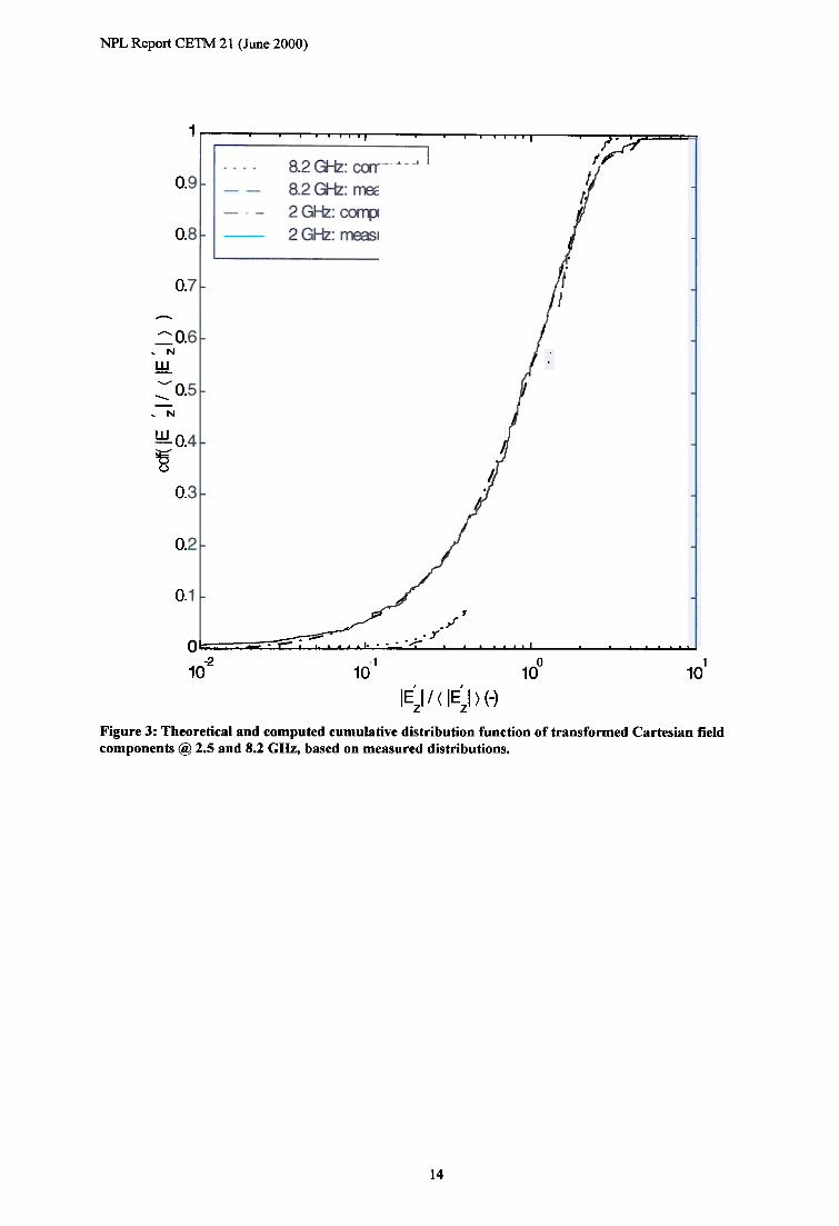
Figure 3: Theoretical and computed cumulative distribution function of transformed Cartesian field components @2.5 and 8.2 GHz, based on measured distributions. 14

..

Figure 4: Measured autocorrelation function of stirrer data after ensemble decimation (pz) and after orthogonalexpansion (Pz) @ 8.2 GHz. 15

......... 3.

.

NPL Report CETM 21 (June 2000)

..

1. Introduction

.

The statistical modelling of electromagnetic reverberation chambers is a powerful and robustanalysis technique that assists in the EMC compliance and pre-compliance testing in suchchambers [1]. However, the technique has uncertainties of various origins associated with it.Under proper reverberation conditions it enables uncertainties for the estimated maximum fieldof :t1.5dB or better to be attained, at the 95%-confidence level, at a single location of the EUT[2]. For certain EMC applications, the uncertainty levels may be required to be further reducedstill, in particular for small sample sizes aimed at shortening test cycles or for operation atrelatively low frequencies.

In this report, we address the reduction of the uncertainty caused by the tuner dataautocorrelation and the test variability. Data correlation makes the statistical characterization ofthe stirring process considerably more complicated.

..

2. Uncorrelated sampled data

.

A typical statistical analysis of measured reverberation chamber data starts with the calculationof the autocorrelation function (act) pC't') of the mode stirring or mode tuning process with stirvariable 't'. On this basis, an 'equivalent' number of 'independent' samples Neq is estimatedfrom M data points associated with M stirrer positions or sample locations. This then allowsone to estimate statistics of the local magnitude or power density of the total field or arectangular field component (e.g. maximum-to-mean ratio).

...

It has been recognized that a commonly used criterion for 'un'correlatedness, viz. thecorrelation distance 'r in the stir domain as defined by:

eq

.

(1)

.

is heuristic and is being used ad hoc [2]-[5]. Its lack of a rigorous foundation does not allowfor accurate estimates of Neq. Indeed, alternative criteria exist [2,5], defined in the stir domainor in the spectral stir domain, which yield substantially different estimates for Neq but which arenevertheless of similar appeal. Moreover, the sample correlation distance has been found toexhibit variation as a function of sample size [5], again affecting the estimation of Neq. Thus,defining criteria for uncorrelatedness with proper foundation is important in its own right.

.

In addition, field statistics have an inherent uncertainty associated with them. Although forrealistic values of N the standard deviation and confidence intervals of the field statistics are

eqoften within acceptable ranges, this presumes the value of N eq to be known with sufficientaccuracy. In view of the arbitrariness of the above or other criterion of uncorrelatedness, thisaccuracy is questionable when using one or other defmition for the correlation distance.Consequently, the uncertainty on Neq adds to the uncertainty on the field statistics themselves(as applicable for a known value of Neq under adequate reverberation conditions) and to theclassical measurement uncertainty of deterministic fields, thus giving rise to an expandeduncertainty. The effect becomes of particular concern in the trend towards using smallervalues of M and N eq for chamber operation and EUT testing to shorten test cycles and reduce

.... 4

.

NPL Report CETM 21(June 2000)

.

cost. Fig 1 illustrates the expanded uncertainty for ideal reverberation chamber data due to theuncertainty on Neq which is estimated to range between Neq = 40.. .60 by way of example. Ascan be seen, the resulting uncertainty on the bounds of the 95%-confidence interval for themaximum-to-mean ratio can be considerable, in this case about 10%.

...

In this paper, we present two transfonnation methods that enable the uncertainty on Neq to bereduced and, for large M, to be asymptotically eliminated. The first method is relatively simple,but does not address the ambiguity of the criteria for uncorrelatedness. The second method isrigorous, but requires greater computational effort. For the latter, a distinction is also madebetween sample decorrelation and ensemble decorrelation.

....

3. Ensemble decimation

..

In conventional sample decimation, the tuner data is subsampled at a rate corresponding to thecorrelation distance in the original measured sample, on the basis of an a priori chosen criterionfor uncorrelatedness such as (1). For improved decimation accuracy, ensemble decimationfactors can be calculated based on the ensemble acf. This eliminates sample variability in theassociated decimation factor, yielding a more reliable value for chambers with variableboundary conditions between tests, e.g. with different EUTs in place or with EUTs in differentchamber locations and orientations.

....

The method is based on the application of the Wiener-Khinchine theorem for the powerspectral density function (psdf) [5,6]. A 3rd-order exponential interpolation was used to obtaina filtered psdf. It thus appears that the normalized one-sided psdf can be modelled to goodapproximation as g(w) = f3 exp(-f3w) for CO>O, where f3 is a spectral parameter characterizingthe ensemble stirring process. Such an ensemble characterization achieves minimum bias in theestimation. The inverse Fourier cosine transformation of g( w) then yields the ensemble acf:

.....

(2)

.

from which the ensemble correlation length and decimation factor follow, e.g. with (1) thisyields 'l'.q = pV(e-l). The merit of the technique is in the fact that the ensemble decimationfactor is obtained from a single representative sample acf.

..

Fig 2 shows a typical single-sample act and associated psdf, as measured in the NPL stadiumreverberation chamber at 8.2 GHz in mode-tuned operation for a stirrer step L1'f. Thecorresponding ensemble act and psdf are also shown. More refined models for the psdf andstirring process often lead to nonlinear estimation problems for the spectral parameter(s).

....

4. Orthogonal expansion

.

4.1 Sample orthogonalization

..Orthogonal expansions are possible for stationary as well as non-stationary processes, whichmay have a Gauss normal distribution or other. In this method, the sample data are maximallydecorrelated, for a given sample size M with arbitrary N eq' using an eigenvalue decomposition.A I-dimensional sequence of discrete stirrer data Xl is expanded as:

... 5.

NPL Report CElM 21 (June 2000)

..

(3)

..

M-l

Xk = Laml/Jmk(T)8(T+ T/2- k/!T), -T/2 ~ T ~ T/2m=O

T/2

am = J Xkl/J;k (T)c5( T + T/ 2 -k/!T)dT-T/2

(4)

.

where T is the length of the tuner (stirrer) sweep interval in units 11'l' and where the Mxl-vectors <!>m = [<!>mk( 'l')£5( 'l'+ T/2-k11'l')] form a complete orthonormal set, chosen such that «(am-(aj)*(an-(an») = Am28mn' Upon substituting (4), the Am2 and <!>m for standardized Xk are found as the

eigenvalues and associated eigenvectors, being solutions of the matrix eigenvalue equation:

....

(5)

.

in which R is the MxM data autocorrelation matrix and I is the MxM unit matrix. For a wide-sense stationary stirring process, R is Hermitian so that all Am2 are real positive scalars.Furthermore, all t/Jm are then real vectors, hence if the data Xk have a complex Gauss normaldistribution (e.g. for measured complex ideal reverberant fields), then the random expansioncoefficients am also exhibit a complex Gauss normal distribution, by virtue of (3). In this casethe uncorrelated am, generally defining a white process, are furthermore statisticallyindependent, so that the lamF exhibit a X: distribution:

.....

(6)

.

For the 3-dimensional (vector) stirring process of interest, the cfJmk( -r)l5( -r+ TI2-kL1r) arethemselves lx3-vectors, but the am remain scalar. For mode-stirring, as opposed to mode-tuning operation, each lx3-vector Xl is itself an average across the width of the samplingwindow. In general, this averaging affects their distribution as compared to the point values.For multiple measurements, the probability density functions of the mean field magnitude I~or mean power density P associated with a Cartesian field component (a = x,y,z) or with thetotal field (t) then follow upon inverse Fourier transformation of the respective characteristicfunctions associated with the 1:.laml as:

......

f Pa (Pa) = 71 l)(l+jWAm)-l]exP(j"Pa)dW (7)

..

f p, (PI) = 11 Q (1 + imAm) -3] exp(JQJJI )dm (8)

...

.tiEal (leal) = 71 IJ'I'm(m) ]eXP(jmleal)dm (9)

.J11}

(m(W) ] exp(jml et I)dm!jEt I (letl) = (10)

... 6

.

NPL Report CETM 21(June 2000)

.

with

.

-] ]exp[

.

2im).,m

21/fm(m) = 1+

.'dz

ex{2

+~

.

z~(m) =2

..

The corresponding cumulative distributions functions (cdfs) are obtained by replacing thefactor exp(j{£fJa) etc. in (7)-(10) by [exp(j{£fJa)-I]/(j{JJ) etc. These expressions now allow for acomparison with ideal X2pN(2) distributions (p = 1,2,3) for the field magnitude or power densityof statistically independent data [8], as is usually assumed ad hoc. Note that the existence ofthe pdfs (7)-(10) presume R to be positive definite, whereas the existence of the cdfs onlyrequire R to be positive semi-definite [10].

....

We have applied the technique to the mode-tuned operation of our chamber by solving theeigenvalue problem (5) numerically. In general, this requires the inversion of a large MxM-matrix. However, this is not required for the problem at hand if M ~ 00 or if the acf issufficiently simple, as will be demonstrated next.

...

If the sample acf p(L\'t") and associated sample autocorrelation matrix R(L\'t") are used, and if adecomposition (decorrelation) is required only for the wide-sense stationary process associatedwith a large set of sample stirrer data, then the eigenvalue problem can be solved semi-analytically because of the circulant natUre of the Toplitz matrix R under stationary conditions[2,7]. In the limit M ~ 00 and arbitrary nonzero L\'t", the eigenvalues are found as:

....

M-l~ = L Rlk exp(jkOJm)

k=O

.

where R1, the [lIst row of R, is the sampled, i.e. discrete acf; (J)m = 2m/M with m = 0,1,..and with associated eigenvectors which are independent of R1k:

..

l/>m = [l;exp( -jmm);exp( -j2mm);...;exp( -j(M -l)mm)] /..{M

..

The vector of transformed measured stirrer data, [Xk'] = [cpkm]+. [Xm], then follows as [2]:

.

Xo

..

Xl = lfl/2

.

XM-l

..which become asymptotically uncorrelated when M ~ 00. Thus, as a result of R beingcirculant, the orthogonal transformation is asymptotically equivalent to a unitary discrete

... 7.

.

NPL Report CE1M 21 (June 2000)

.

Fourier transfonnation, for which a fast implementation is readily available. Consequently, theuncorrelated field is asymptotically obtained as the unitary Fourier transfonned field.

..

Sample orthogonalization is recommended if the measurement or test set-up changes very littleor not at all between tests (viz. for identical stepping or rotational speed of the tuner per testcycle, identical stirrers and antennas with fixed orientations, fixed cable layout, identical type,position and orientation of EUTs etc.), or if only a single assessment is required. Theseconditions may be difficult to meet in practical EMC tests. In this case, ensembleorthogonalization may be more appropriate.

....

4.2 Ensemble orthogonal;zat;on

..

Here the parameters of the stirring process x( -r) have been changed, due to differences instirring step or speed, chamber reconfigurations including stirrer alterations, etc., or the EUT isleft unspecified or is repositioned in between tests. Hence sample orthogonalization is nolonger appropriate. In this case, the method used in the ensemble decimation procedure can beapplied, prior to performing the orthogonal expansion. The ensemble psdf then yields theensemble acf for constructing the kernel of the eigenvalue problem. When choosing a rationalfunction to model the psdf, viz. g(ro) = 4y/ (cJ+i) with spectral parameter y; the ensemble acfcan be expressed in closed form and yields an integrable kernel for the eigenvalue equation.The orthogonal expansion now reads:

......

M-I T/2

X( 't") = IamC/>m( 't"); am = Jx( 't")C/>;( 't")d't"m=O -T/2

(16)

.

where the continuous eigenfunctions CPm( 't) are now solutions of a linear homogeneousFredholm integral equation of the second kind:

..

T/2

J p( 'l' , V)l/Jm (V )dv = ~ l/Jm ( 'l')-T/2

(17)

..

With the associated acf p( 't, v) = (1r/2) F c-l[g(m)] = exp(-~'t-~), the transfonned stiITer data canbe obtained analytically, which is advantageous in applying the orthogonalization procedure inpractice. The eigenfunctions are found upon twice differentiating (17) and solving the resulting2nd-order differential equation as:

..

-1/2

f [ sin(fJT ~2(J'2 / (fJ~m+l )-1)4>2m+l("C) = f 1+ fJT~2(J'2 /(fJ~m+l)-1

.

(18)

.

-1/2

.

sin( fJ'l" .J20' 2 / (fJA;m ) -1 ) ~l~)

.Both subsets of eigenfunctions (18)-(19) become asymptotically harmonically related in thelimit 1JFV[2d/({3Am2)-I] ~ 00. The associated eigenvalues Am2 are found from the iterativesolution of the characteristic equation:

.. 8

.

NPL Report CETM 21(June 2000)

...

~T 20' -1t1 j3""2 Iii;;: :!: =0 (20)

..

For general p( 'l"- v), the Am2 are monotonically increasing functions of T. In the limit T ~ 00,they form a continuum A1w) that coincides with g(w) and the tPm('l") then tend to exp(j(J)'l"). Forthe full 3-dimensional stirring process, the tPm(t) are lx3-vector eigenfunctions.

..

The results (18)-(20) apply to the analytical modelling of the continuous stirring process x('i),based on measurements in our chamber, and again avoid the need for solving the integralequation (17) numerically. For more general acfs, the integration can still be performedprovided (17) has a separable Pincherle-Goursat kernel of finite order, in which case theequation can always be reduced to a system of linear algebraic equations. For a wide-sensestationary stirring process, this kernel is Hermitian i.e. p( 'i, v) = p. (v, 'i), so that the Am2 are realpositive and the tf>m( 'i) are real, as noted in Sec 4.1.

.....

5. Examples

.

We applied the above techniques to measured mode-tuned reverberation data as collected inthe NPL untuned stadium reverberation chamber (diameter d = 70 cm) [2,3,5,6] at 2 GHz and8.2 GHz, corresponding to d/A = 4.67 and 19.13, thus yielding a relatively low and high mode

density, respectively.

...

In Fig 3, the dashed line shows the measured cdf for the mean-normalized amplitude of amean-normalized rectangular field component IEzV<IEJ) at 8.2 GHz, after ensemble decimationwith decimation factor mz = 4, obtained using the p-l( e-1 )-criterion. For comparison, the dottedline shows the theoretical Xz cdf for ideal reverberation chambers. The good agreementbetween both cdfs indicates adequate reverberation performance at this frequency, withdecimation being sufficient for obtaining approximately independent samples. The solid lineshows the measured cdf at 2 GHz, obtained as an average over 25 measurement locations withM = 1200 per location. This distribution is to be compared with the theoretical cdf (dot-dashedline), obtained using the sample orthogonalization as [Ez'] = [tf>km]+ .[Ez] and based on themeasured acf kernel. The transformed fields fully justify a comparison with a theoretical cdfbased on independent samples. This, then, enables various field statistics to be estimated more

accurately.

........

Fig 4 compares the magnitude of the sample acf Pz (crosses), after sample decimation, with theone for sample orthogonalization, Pz' (diamonds). As can be seen from a comparison of thevalues of the acf for the flfst two stirrer positions, the correlation distance afterorthogonalization is only about a quarter of the corresponding value for the decimated data,regardless of the choice of the threshold for uncorrelatedness. The Figure effectively indicatesthat the value of N.q, estimated using sample decimation as N.q = M/mz = 300, is beingoverestimated and that orthogonalization gives rise to superior decorrelation.

....... 9.

.

NFL Report CElM 21 (June 2000)

..

6. Conclusions

..

We have shown how ensemble decimation and orthogonal expansion of stirrer data can lead toimproved estimates of the equivalent number of independent samples and sample statistics ofthe field magnitude and power density.

..

Ensemble decimation uses the psdf rather than the measured psdf to improve on the estimatedlevel of data correlation, hence it serves in reducing the test variability and in improving thetest reproducibility. Recall that uncorrelated data are merely linearly independent, unless theyobey a Gauss normal distribution in which case uncorrelatedness guarantees statistical (i.e.linear as well as higher-order nonlinear) independence. Decimation or orthogonal expansion ofstirrer data representing field magnitude or power density, obeying non-Gaussian distributionsas opposed to complex field data, may therefore leave residual nonlinear dependencies betweenthem.

....

Orthogonal expansion was found to yield superior data decorrelation. For arbitrarily largesample sizes, the orthogonal expansion asymptotically reduces to a discrete Fouriertransformation of the acf for stationary data, i.e. a transformation of the stirrer data into theFourier spectral stir domain. In practice, the accuracy of such approximation depends on thelength T = MAT of the stir interval relative to the calculated scale of fluctuation (JT of thestirring process [5]. The orthogonal expansion is furthermore useful in studying the distributionfunction and statistics of the actual field magnitude or power density, especially for moderatelevels of mode density. The accuracy of the estimated distribution function rests on theaccuracy of the modelling of the autocorrelation function or the power spectral density of thestirring process. Furthermore, the technique enables one to determine the effect of local stiraveraging and, by extension, local spatial averaging on the change in the distribution functionof the stirrer data. This is of considerable importance in determining level crossing statistics forEMC and EUT failure testing [2,5,6].

........

The above analysis has concentrated on data autocorrelation, ignoring the cross-correlation thatmay exist between in-phase and quadrature or between Cartesian field components. Thesecross-correlations can be eliminated along similar lines, by requiring «am-(aJ)* (bn-(bn»)) =Am28mn for the expansion coefficients am and bn of the components. In an alternative approach,the cross-correlation between the field components can be taken into account explicitly via acorrelation coefficient [9]. This method requires an estimate for the thus introduced additionalstatistical parameter.

.......... 10

.

NPL Report CE1M 21(June 2000)

..

7. References

..

[1] Lehman, T H and Freyer, G J: Characterization of the maximum test level in areverberation chamber; IEEE Symposium on EMC 1997 (18-22 Aug 1997, Austin, TX), pp 44-47.

..

[2] Arnaut, L R and West, P D: Evaluation of the NPL untuned stadium reverberation chamberusing mechanical and electronic stirring techniques, NPL Report CEM 11 (Aug 1998).

.

[3] Arnaut, L R: Untuned 3D stadium reverberation chamber for microwave and millimeter-wave frequencies, Mode-stirred Chamber, Anechoic Chamber and OATS Users Meeting 1999,(7-9 Jun 1999, Northbrook, IL).

..

[4] Lunden, 0, Jansson, L and Backstrom, M: Measurements of stirrer efficiency in mode-stirred reverberation chambers; FOA Swedish Defence Research Establishment Report FOA-R-9901139-612-SE (May 1999).

..

[5] Arnaut, L R and West, P D: Electric field probe measurements in the NPL untuned stadiumreverberation chamber, NPL Report CETM 13 (Sep 1999).

..

[6] Arnaut, L R and West, P D: Effect of antenna aperture, EUT and stirrer step size onmeasurements in mode-stirred reverberation chambers, IEEE Symposium on EMC 2000 (21-25Aug 2000, Washington, DC).

..

[7] Grenander, U and Szego, G: Toplitz forms and their applications; 2nd ed, Chelsea Publ,NY (1984).

..

[8] Spiegelaar, H and Vanderheyden, E: The mode stirred chamber -a cost effective EMCtesting alternative, IEEE Symposium on EMC 1995 (21-25 Aug 1995, Atlanta, GA), pp 366-373.

..

[9] Lehman, T H, Freyer, G J, Hatfield, M 0, Ladbury, J M and Koepke, G H: Verification offields applied to an EUT in a reverberation chamber using numerical modeling, IEEESymposium on EMC 1998 (24-28 Aug 1998, Denver, CO), pp 28-33.

...

[10] Wong, E and Hajek, B: Stochastic Processes in Engineering Systems,' Springer Verlag,NY (1985).

......... 1.

NFL Report CETM 21 (June 2000)

8. Figures

N =4)EIj

N =8)EIj

N =00EIj

..

'",

.

\\

.

\ '.

..

\

,

c

\

.

~

i~fl)~"§~~Q5'B:

\

.

\ "

( f

II:.j Ir "

I "II, ., ' ,

.1 .II

1.5 2 2.5 3 3.5

rTB« IE 1/( IE I) ) (-)z z

4 4.5 5

Figure 1: Theoretical probability density functions, 2.5% and 97.5% percentiles of maximum- to-meanfield strength for Cartesian field components for various Neq.

......... 12

.

NPL Report CElM 21(June 2000)

..

RJI-s aJcmT'Bctim ftn::tim

~"""'I """,':=:- ~nJe~ei,- amTtie I

.

a8

.

_a6~

~_a4

~-No.a2

...

J~ -'. -~ J(\'~r'\I,~'~~I~il\ I ", I r

I ~ \ ~'" J ",f \ \,- \w-

-0.21 , ...1 ..,. I ""0 1 2

10 10 10

.

""

...........

Figure 2: Single-sample and ensemble autocorrelation function and power autospectral density functionfor Cartesian field component @ 8.2 GHz.

............. 13.

.

NFL Report CE'IM 21 (June 2000)

..

.11 .., , ,."..,', '/~:J.:r

..

0.9

.

0.8

..

0.7

.

"""'0.6, N

~""""0.5-

, N

~0.4

~0.3

..

jj

J

J

.;f

.1

.rJ

....

0.2

.

(I

.

.J0..f

I- =--:--;::;:.~~~'~~ .~ ..;;..0 f. ..,.10 ~ ., , , , I '" ,0 ~ of.0 .." " " " ".;:..

-2 -1 0 110 10 10 10

....

IE 1/< IE' I ) (-)z z

Figure 3: Theoretical and computed cumulative distribution function of transformed Cartesian fieldcomponents @ 2.5 and 8.2 GHz, based on measured distributions.

............ 14

.

NPL Report CETM 21(June 2000)

..................

t/d t+1

.

Figure 4: Measured autocorrelation function of stirrer data after ensemble decimation (PJ and afterorthogonal expansion <Pz'> @ 8.2 GHz.

............ 1 ~