Decision Forests with Long-Range SpatialContext for Organ Localization in CT Volumes

A. Criminisi, J. Shotton, and S. Bucciarelli

Microsoft Research Ltd, Cambridge, UK

Abstract. This paper introduces a new, efficient, probabilistic algo-rithm for the automatic analysis of 3D medical images. Given an in-put CT volume our algorithm automatically detects and localizes theanatomical structures within, accurately and efficiently.Our technique builds upon randomized decision forests, which are enjoy-ing much success in the machine learning and computer vision communi-ties. Decision forests are enriched here with learned visual features whichcapture long-range spatial context. In this paper we focus on the detec-tion of human organs, but our general-purpose classifier might be trainedinstead to detect anomalies. Applications include (and are not limitedto) efficient visualization and navigation through 3D medical scans.The output of our algorithm is probabilistic thus enabling the modelingof uncertainty as well as fusion of multiple sources of information (e.g.multiple modalities). The high level of generalization offered by decisionforests yields accurate posterior probabilities for the localization of thestructures of interest. High computational efficiency is achieved thanksboth to the massive level of parallelism of the classifier as well as the useof integral volumes for feature extraction.The validity of our method is assessed quantitatively on a ground-truthdatabase which has been sanitized by medical experts.

1 Introduction

This paper presents a new, efficient algorithm for the accurate detection andlocalization of anatomical structures within CT scans. This work represents asignificant step towards automatic parsing and understanding of medical images.

Our effort is motivated by recent studies which indicate how the great ma-jority of a radiologist’s time is spent searching through scanned volumes (oftenslice by slice) and navigating through visual data. Even with modern 3D visual-ization tools locating the organ(s) of interest and selecting optimal views is timeconsuming. Automatic tools for localizing major anatomical structures within3D scans promises to speed up navigation and improve the user’s work-flow [1].For instance, a cardiologist may just click on a button to take him/her to themost appropriate view of the heart and its valves. Robust and efficient, proba-bilistic organ detection is also useful as input to other, more specialized tasks,e.g. detecting the heart to initialize a coronary tree tracer tool.

The two main contributions are: 1) We introduce an efficient algorithm fororgan detection and localization which negates the need for atlas registration;

thus overcoming issues related to, e.g. : i) possible lack of atlases, and ii) selectingthe optimal model for geometric registration. 2) We introduce new, context-rich visual features which capture long-range spatial correlations efficiently. Thesimplicity of our features combined with the intrinsic parallelism of our classifieryield high computational efficiency. Finally, our algorithm produces probabilisticoutput, useful for instance to keep track of uncertainty in the results, to takeinto account prior information (e.g. about global location of organs) or to fusemultiple sources of information (e.g. different acquisition modalities).

The proposed algorithm is applied here to the task of localizing nine anatomi-cal structures (head, heart, left eye, right eye, l. kidney, r. kidney,l. lung, r. lung, and liver) in CT volumes with varying resolution, vary-ing cropping, different patients, different scanner types and settings, contrastenhanced and not etc. Quantitative assessment is executed on a number of man-ually labelled ground-truth CT volumes.

Previous work. In the last few years research in object detection and recogni-tion has made huge progress. The published work which is relevant to medicalapplications may be broadly categorized into the following three groups:

Geometric methods include template matching, and convolution techniques [2].Geometrically meaningful features are used in [3, 4] for the segmentation of theaorta and the airway tree, respectively. Such geometric approaches often haveproblems capturing invariance with respect to deformations (e.g. due to patholo-gies), changes in viewing geometry (e.g. cropping) and changes in intensity. Tech-niques built upon “softer” geometric models with learned spatial correlationshave been demonstrated to work well both for rigid and deformable objects [5].

Atlas-based techniques have enjoyed much popularity. Recent techniques for sin-gle and multiple organ detection and segmentation based on the use of probabilis-tic atlases include [6–10]. The apparent conceptual simplicity of such algorithmsis in contrast to the need for accurate, deformable registration algorithms. Themajor problem with n-dimensional registration is in selecting the appropriatenumber of degrees of freedom of the underlying geometric transformation; espe-cially as it depends on the level of rigidity of each organ/tissue.

Supervised, discriminative classification. Discriminative classification algorithmssuch as Support Vector Machines (SVM), AdaBoost and Probabilistic BoostingTrees have been applied successfully to tasks such as: automatic detection of tu-mors [11–14], pulmonary emphysema [15], organs in whole-body scans [19] andbrain segmentation [16–18]. Our approach is also a discriminative classificationtechnique. It achieves multi-class recognition efficiently and probabilistically. Theclassifier employed here is a random decision forest which, in non-medical do-mains has been shown to be better suited to multi-class problems than SVMs,as well as being more effective than boosting [20, 21]. A model of spatial contextis learned by automatically selecting visual features which capture the relativeposition of visual patterns. Next we describe the details of our technique.

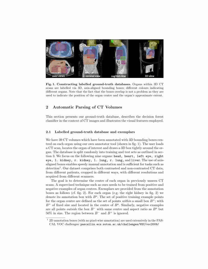
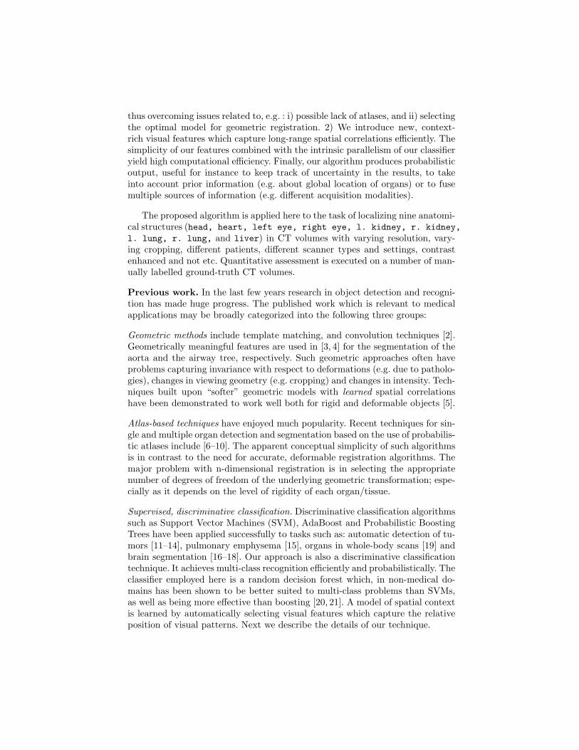
Fig. 1. Constructing labelled ground-truth databases. Organs within 3D CTscans are labelled via 3D, axis-aligned bounding boxes; different colours indicatingdifferent organs. Note that the fact that the boxes overlap is not a problem as they areused to indicate the position of the organ centre and the organ’s approximate extent.

2 Automatic Parsing of CT Volumes

This section presents our ground-truth database, describes the decision forestclassifier in the context of CT images and illustrates the visual features employed.

2.1 Labelled ground-truth database and exemplars

We have 39 CT volumes which have been annotated with 3D bounding boxes cen-tred on each organ using our own annotator tool (shown in fig. 1). The user loadsa CT scan, locates the organ of interest and draws a 3D box tightly around the or-gan. The database is split randomly into training and test sets as outlined in sec-tion 3. We focus on the following nine organs: head, heart, left eye, righteye, l. kidney, r. kidney, l. lung, r. lung, and liver. The use of axis-aligned boxes enables speedy manual annotation and is sufficient for tasks such asdetection1. Our dataset comprises both contrasted and non-contrasted CT data,from different patients, cropped in different ways, with different resolutions andacquired from different scanners.

The goal is to determine the centre of each organ in previously unseen CTscans. A supervised technique such as ours needs to be trained from positive andnegative examples of organ centres. Exemplars are provided from the annotationboxes as follows (cf. fig. 2). For each organ (e.g. the right kidney in fig. 2) wedenote its annotation box with Ba. The set of positive training example pointsfor the organ centre are defined as the set of points within a small box B+; withB+ of fixed size and located in the centre of Ba. Similarly, negative examplesare all points outside the box B− with same centre and aspect ratio as Ba but50% in size. The region between B− and B+ is ignored.

1 2D annotation boxes (with no pixel-wise annotation) are used extensively in the PAS-CAL VOC challenges: pascallin.ecs.soton.ac.uk/challenges/VOC/voc2009/

Fig. 2. Positive and negative training examples. (a) A 3D view illustrating theground truth annotation box Ba, the box of positive examples B+ and the box ofnegative examples B−. (a) A 2D view further clarifying the regions where exemplarsfor the organ centre are taken. Positive examples are sampled within the box B+ (ingreen). Negative example points are sampled outside the box B− (in red).

2.2 Decision forests for recognition in 3D medical images

This section describes our adaptation of decision forests to the task of organdetection and localization in 3D CT scans.

A random decision forest [23, 24] is a collection of deterministic decision trees.Decision trees are popular classification algorithms which are known to sufferfrom over-fitting (poor generalization). Recently, it has been shown that theensemble of many randomly trained decision trees (a random forest) yields muchbetter generalization while maintaining the advantages of conventional decisiontrees [23]. Intuitively, where one tree fails the others do well.

We use the following notation. A voxel in a volume V is defined by its coordi-nates x = (x, y, z). The forest is composed of T trees denoted Ψ1, · · · , Ψt, · · · , ΨT ;with t indexing each tree (fig. 3). In each tree, each internal node (split node)performs a binary test on the input data and based on the result directs thedata to the left or right child. The leaf nodes do not perform any action, theyjust store probability distributions over the organs of interest. Next we describehow the split functions are chosen and how the leaf probabilities are computed.Forest training. Each point x of each training volume is associated with aknown (manually obtained) class label Y (x). The label indicates whether thepoint x belongs to the positive set of organ centres (see fig. 2) or not. Thus,Y (x) ∈ { head, heart, left eye, right eye, l. kidney, r. kidney, l.lung, r. lung, liver, background }, where the background label indicatesthat the point x is not an organ centre.

During training T is fixed (we use T = 10). Then, each point x is pushedthrough each of the trees starting at the root. Each split node applies the follow-ing binary test: ξ > f(x; θ) > τ and sends the data to the respective child node.f(·) is a function applied to x with parameters θ. The parameters θ identify thevisual features which needs be computed. Features are described in the next sec-tion; for now it suffices to say that f computes some scalar filter response at x.ξ and τ are parameters of the split node. The purpose of training is to optimize

Fig. 3. Random Decision Forests. (a) An example random decision forest made of3 trees. In each tree the internal nodes (shown with ellipses) perform simple tests onthe input data while the leaf nodes (shown as squares) store the posterior probabilitiesover the classes being trained. During testing, a data point is pushed simultaneouslythrough all T trees until it reaches T leaf nodes. The probability assigned to that pointis the average of the probabilities of all the reached leaves (see text). (b) Each internalnode performs a simple binary tests on the input data x, based on the feature responsef(x; θ). The quantities ξ, τ and θ are parameters of the splitting test in that node.

the values of θ, ξ, τ of each split node by maximizing the data information gain,just like in the standard C4.5 tree training algorithm [25].Injecting randomness for improved generalization. However, unlike standard treetraining methods, here the parameters of each split node are optimized only overa randomly sampled subset Θ of all possible features (here |Θ| = 500, details insection 2.3). This is an effective and simple way of injecting randomness into thetrees, and it has been shown to improve generalization.

During node optimization all available features θi ∈ Θ are tried one afterthe other, in combination with many discrete values for the parameters ξ andτ . The combination ξ∗, τ∗,θ∗ corresponding to the maximum information gainis then stored in the node for future use. The expansion of a node is stoppedwhen the maximum information gain is below a fixed threshold. This gives riseto asymmetrical trees which naturally stop growing when no further nodes areneeded. In this work the maximum tree depth D is fixed at D = 15 levels.

Finally, by simply counting the labels of all the training points which reacheach leaf node we can associate each tree leaf with the empirical distributions overclasses Plt(x) (Y (x) = c), where lt indexes the leaf node in the tth tree (fig. 4f).This training procedure is repeated for all T component trees.Testing. During testing each point x of a previously unseen CT volume issimultaneously pushed through each of the T trees until it reaches a leaf node.Thus, the same input point x will end up in T different leaf nodes, each associatedwith a different posterior probability. The output of the forest, for the point x,is the mean of all such posteriors, i.e. :

P (Y (x) = c) =1T

T∑t=1

Plt(x) (Y (x) = c) . (1)

Other ways of combining the tree posteriors have been explored and simpleaveraging appears to be the most effective (as demonstrated also in the vastliterature). Also, analyzing the variability of individual tree posteriors carriesuseful information about the uncertainty of the final forest posterior.Organ detection. At this point detecting the presence/absence of an organ c isdone simply by looking at the max probability Pc = maxx P (Y (x) = c). Theorgan c is considered present in the volume if Pc > β, with β = 0.5.Organ localization. The centre of the organ c is estimated by marginalizationover the volume V :

xc =∫

V

x p(x|c) dx, (2)

where the likelihood p(x|c) = P (Y (x) = c) by using Bayes rule and assuminguniform2 distribution for organs. Furthermore, maximum a-posteriori classifi-cation for each voxel x may also be obtained as: c∗ = arg maxc P (Y (x) = c).After having described our classification algorithm, next we provide details ofthe visual features employed.

2.3 Visual features and learned spatial context

The problem with identifying anatomical structures in CT images is that differ-ent organs may share similar intensity values. Thus, local intensity informationis not sufficiently discriminative and further information such as texture, spatialcontext and topological cues must be used to have any chance of success. Theproblem then is how to capture and model such information efficiently.

Here we consider visual features which capture both the appearance of anatom-ical structures as well as their relative position (context) within the decisionforest framework. For each location x context is modeled by integrating infor-mation coming from multiple regions which are offset by a quantity ∆ in agiven direction. Figures 4 explains the main concepts with a 2D illustration.A feature θ is defined as a reference point o paired with two boxes F1, F2

and two signal channels C1, C2. The shapes Fi are just 3D boxes displacedwith respect to o. The channels Ci could be for example the CT intensity(C(x) = I(x)), or the magnitude of the 3D gradient (C(x) = |∇I(x)|). Givena point x in a volume, computing the feature response f(x; θ) corresponds toaligning the reference point o of the feature θ with the point x and computingf(x; θ) =

∑q∈F1

C1(q) − b∑

q∈F2C2(q). The parameter b ∈ {0, 1} indicates

whether both feature boxes are used or only one (in fig. 4 b = 0 for simplicity).As shown in fig. 4 these features tends to capture the relative layout of visual

patterns (e.g. kidney patterns tend to occur a certain distance away, in a certaindirection, from liver patterns, fig. 4d). The use of rectangular regions enablesefficient integral volume processing [29, 30, 16]. Our features may be thoughtof as a generalization of the Haar-like features used in [26, 30, 16, 17]. In fact,we do not use manually predefined Haar subdivisions of a canonical cuboid.Our classifier is free to select features with very large offsets ∆, which enables2 Alternatively one can weight each class based on its own volume in the training set

Fig. 4. Context-rich visual features, a 2D illustration. (a) Coronal view of apatient’s abdomen. (b) Features (denoted θi) are defined as the rigid pairing betweena box F and a reference point o. Here we show only some of the infinite possible features.In practice we use 3D axis-aligned boxes. (c) Computing the feature response f(x; θ)at position x within a volume corresponds to aligning o with x and computing the sumf(x; θ) =

∑q∈F I(q) (cf. text. For simplicity here we use intensity as the channel and

only one rectangle). For feature θ13 when o is on the kidney the rectangle F is in aregion of low density (air). Thus the value of f(x; θ) is small for those points. Duringtraining the algorithm will learn that feature θ13 is discriminative for the position ofthe right kidney when associated with a small, positive value of the threshold ξ13 (withτ13 = −∞). The region for which the condition ξ13 > f(x; θ) > τ13 is true is shownin green. (d,e) Similar to (c) but with different features. (f) Training associates eachnode with optimal values of ξ, τ,θ. In this example, a data point which follows thehighlighted path (in blue) gets assigned a high probability of being the centre of akidney. (g) The points which satisfy all three conditions in (f) lie in the intersectionof the three regions (c, d, e), highlighted in dark green, inside the organ of interest.

capturing very long-range spatial interactions. Inspection of the trained treesreveals that often the ∆ of selected features can be as large as the image width.For simplicity, in this paper we only consider intensity and gradient as channels.However, our features are more flexible and general than that as they allow toincorporate complex filters such as SIFT, HOG etc. Multiple modalities mayalso be exploited; e.g. in the case of MR one may use T1, T2, FLAIR etc. Morecomplex visual cues such as the ones described in [27, 28] or differently shapedaggregation regions may also be employed.

During training, for each split node the set Θ is obtained by randomly gener-ating for each feature the two boxes F1, F2 (e.g. their centre and dimensions arerandomly selected) and the corresponding channels C1, C2. Then all nodes areoptimized and once training completes the trees, their nodes and the selectedfeatures are frozen and the testing phase proceeds deterministically.

2.4 Discussion and comparisons

The classifier used here is related to the Probabilistic Boosting Tree in [16]. Inour case, the tree nodes contain test functions that are simpler than the boostersused in [16], with advantages in terms of speed both during training and testing.Furthermore, as shown in [20], a collection of simple, randomized trees tends toyield better generalization than a single tree of boosters.

In [17] the authors capture context by means of an algorithm which at eachiteration uses the posteriors of the previous iteration as features. This producesgood results at a cost of multiple iterations. Our algorithm is not iterative andcaptures spatial correlations of visual patterns, namely “appearance context”.Furthermore, our kernels have much longer range. Finally, we do not requirepreregistration of the CT volumes.

Localizing anatomical structures by atlas registration is a popular option.However, such techniques have to deal with issues such as: i) the optimal choiceof degrees of freedom of the registration model (e.g. both fully rigid and fullydeformable transformations are bad); ii) the optimal choice of the reference tem-plate (e.g. an adult male body? a child? or a woman? contrast enhanced or not?);and iii) robustness to anatomical anomalies (training a classifier on data whichpresents anomalies allows the system to learn invariance to those).

The work in [19] makes use of information gain to optimize the schedulingof single-organ boosted detectors. In our work we use information gain at thelevel of feature selection, and detection happens via an ensemble of decision treessimultaneously for all organs. The selected features are organized hierarchically,with the most discriminative ones in the top layers of each tree. This has theadvantage of “sharing” the most discriminative features amongst classes (organs)and sets of classes, with positive effects on generalization (e.g. see [31] for detailson feature sharing and [20] for a detailed comparison between AdaBoost, decisiontrees and decision forests). Next we quantify the performance of the proposedalgorithm and compare it to some known alternatives.

3 Experimental Results and Validation

This section presents qualitative and quantitative assessment of the accuracy ofour algorithm applied to the tasks of organ detection and localization.

3.1 Automatic organ detection and localization

Qualitative results are shown in fig. 5. Our classifier applied to previously unseenCT scans produces accurate posteriors for the location of organ centres. In thesevisualizations the computed posteriors are used to modulate the transfer functionemployed during 3D rendering. For instance, notice how the mass of the heartprobability (in red) is correctly concentrated around the centre of the heartregion. Similarly for the light brown region indicating the liver, etc.Quantitative evaluation of accuracy. Localization accuracy is assessed here byrunning training and testing multiple times. In each round the database is split

Fig. 5. Results of automatic organ detection and localization. (a) The original3D CT data rendered using a manually-designed colour transfer function. (b) Threeviews of the 3D organ posterior probabilities computed by our algorithm for the local-ization problem. Different colours indicate different organs. Larger opacities indicatelarger probability of a voxel being the organ centre. Notice how well eyes (green), head(yellow), heart, lungs, liver and even kidneys (purple) have been localized. A faint bodyoutline is shown to aid visualization. (c) 3D views of the automatically detected bound-ing boxes including the heart and left lung. (d,e) Results on two more test datasets.The different datasets (related to different patients) are cropped differently and havedifferent resolutions.

randomly into a training and a test set (with approximate ratio of 2 : 1). Forall algorithms evaluated in this section the same 10 random splits are used. Theforest is optimized on the training set only, and then applied on the test set.Then, the location of each organ centre is computed and compared with groundtruth. Resulting localization errors collected from 10 runs (with D = 15, |Θ| =500) are shown below (in mm).

organ head heart l. eye r. eye l. kidney r. kidney l. lung r. lung liver mean across organs

median 25.58 18.31 24.04 25.71 13.52 29.49 22.93 21.94 19.01 22.28 mm

mean 29.92 21.32 28.78 27.14 25.42 44.52 27.05 26.75 22.68 28.18 mm

std 12.80 5.67 18.88 18.66 9.82 15.00 7.25 9.44 5.30 11.42 mm

Standard deviations (computed across the means of all runs) are reportedhere only to provide an indication of stability with respect to different train/testsplits. Our algorithm achieves an overall localization error of ∼ 2 cm for median.Eyes show the largest localization uncertainty across different runs (largest std),probably due to their smaller size. Furthermore, the use of larger training setstogether with global position and shape priors [16] promises to improve general-ization across different individuals and anatomies (e.g. missing organs etc.), andincrease both the accuracy and its confidence further.

3.2 Comparisons with other algorithms

Gaussian Mixture Models. For comparison we implemented a GMM-based tech-nique where each organ is modelled by fitting a Gaussian Mixture Model toits distribution of CT intensities. During testing, for each voxel x we evaluatethe probability of that point being the centre of a certain organ c. The centreposition is then estimated as in (2). Localization errors are reported below:

organ head heart l. eye r. eye l. kidney r. kidney l. lung r. lung liver mean acr. organs

median 53.48 88.54 81.56 85.59 133.04 123.38 89.32 89.59 99.63 93.79 mm

mean 144.27 98.32 174.56 168.42 125.55 128.04 104.88 100.29 98.06 126.93 mm

std 95.63 9.55 121.46 114.19 18.70 15.10 8.48 6.19 14.76 44.90 mm

The table above shows much larger errors than with our technique. An analy-sis of the posteriors shows that some organ labels are almost uniformly scatteredspatially. This induces a bias of the detected centres towards the centre of thevolume (thus incorrect), with at times low variance. The reason for such unsat-isfactory results is that the GMM approach is based solely on the organs globalappearance and fails to capture spatial context; and ways of integrating spatialcontext efficiently within a GMM-based approach are not straightforward. Inthis case the use of further features such as gradients did not seem to help much.Template matching. We also compared our technique with a template basedmethod. Here, each organ is represented by a set of 3D templates, extractedfrom the training volumes and each containing the whole organ. During testing,for each organ c we convolve the input volume with all exemplars for that organand select as centre the point associated with the maximum correlation scoreover all exemplar templates. Localization errors are reported below.

organ head heart l. eye r. eye l. kidney r. kidney l. lung r. lung liver mean acr. organs

median 167.53 226.54 96.00 98.53 215.31 343.64 230.12 30.89 96.18 167.19 mm

mean 240.31 191.94 238.12 300.05 229.23 303.29 177.18 134.42 150.46 218.33 mm

std 209.08 24.16 51.33 57.20 33.09 67.33 24.41 40.03 55.15 62.42 mm

In this case the results are still worse than with our technique. We believethis is because rigid templates fail to model variations in object’s shape, scaleand cropping. In this case too the use of gradient features did not help. Finally,as the number of organs of interest increases having to store exemplar templatesbecomes prohibitive, and the processing burden shifts from training to test.

3.3 Computational efficiency

Training our decision forest model on ∼ 26 datasets currently takes around 10hours on an 8-core Intel desktop. We are planning to port the algorithm onto aHigh Performance Computing cluster which should reduce training to only about1 hour. Testing is much faster. In fact, a GPU implementation (following [22])runs in ∼ 2 sec for an approximately 5123 volume.

4 Conclusion

This paper has introduced a new algorithm for the efficient detection and local-ization of anatomical structures within Computed Tomography volumes.

We have presented efficient 3D visual features which capture long-range spa-tial context and help discrimination accuracy. Those features have been incorpo-rated within a random decision forest classifier. The algorithm’s parallel natureand the efficiency of its visual features account for the high computational effi-ciency. The learned model of context accounts for the good localization accuracy.

Next, we plan to extend our technique to other imaging modalities such asMRI, PET-CT and ultrasound. Also, adapting our algorithm to perform hier-archical detection (e.g. thorax → heart → mitral valve) will help dealing withdetailed anatomical structures and will yield richer semantic parsing of medi-cal images. Finally, we would like to extend our work to producing pixel-wisesegmentation of complex anatomical structures such as elongated blood vessels.This will necessitate building pixel-wise annotated ground-truth databases andpromises to deliver useful results.

References

1. Rubin, G.D.: Data explosion: the challenge of multidetector-row CT. EuropeanJournal of Radiology 36(2) (2000) 74 – 80

2. Linguraru, M.G., Summers, R.M.: Multi-organ automatic segmentation in 4Dcontrast-enhanced abdominal CT. In: IEEE Intl. Symp. Biom. Im. (ISBI). (2008)

3. Kurkure, U., Avila-Montes, O.C., Kakadiaris, I.A.: Automated segmentation ofthoracic aorta in non-contrast CT images. In: IEEE Intl. Symp. Biomedical Imag-ing (ISBI). (2008)

4. van Ginneken, B., Baggerman, W., van Rikxoort, E.M.: Robust segmentation andanatomical labeling of the airway tree from thoracic CT scans. In: MICCAI. (2008)

5. Shotton, J., Winn, J., Rother, C., Criminisi, A.: Textonboost for image understand-ing: Multi-class object recognition and segmentation by jointly modeling texture,layout, and context. In: IJCV. (2009)

6. Shimizu, A., Ohno, R., Ikegami, T., Kobatake, H.: Multi-organ segmentation inthree-dimensional abdominal CT images. Int. J CARS 1 (2006)

7. Yao, C., Wada, T., Shimizu, A., Kobatake, H., Nawano, S.: Simultaneous locationdetection of multi-organ by atlas-guided eigen-orgnmethod in volumetric medicalimages. Int. J CARS 1 (2006)

8. Han, X., Hoogeman, M.S., Levendag, P.C., Hibbard, L.S., Teguh, D.N., Voet, P.,Cowen, A.C., Wolf, T.K.: Atlas-based auto-segmentation of head and neck CTimages. In: MICCAI. (2008)

9. Zhuang, X., Rhode, K., Arridge, S., Razavi, R., Hill, D., Hawkes, D., Ourselin, S.:An atlas-based segmentation propagation framework using locally affine registra-tion – application to automatic whole heart segmentation. In: MICCAI. (2008)

10. Fenchel, M., Thesen, S., Schilling, A.: Automatic labeling of anatomical structuresin MR fastview images using a statistical atlas. In: MICCAI. (2008)

11. Dolejst, M., Kybic, J., Tuma, S., Polovincak, M.: Reducing false positive responsesin lung nodule detector system by asymmetric adaboost. In: ISBI. (2008)

12. Pescia, D., Paragios, N., Chemouny, S.: Automatic detection of liver tumors. In:ISBI. (2008)

13. Wels, M., Carneiro, G., Aplas, A., Huber, M., Hornegger, J., Comaniciu, D.: Adiscriminative model-constrained graph-cuts approach to fully automated pediatricbrain tumor segmentation in 3D MRI. In: MICCAI. (2008)

14. Freiman, M., Edrei, Y., Shmidmayer, Y., Gross, E., Joskowicz, L., Abramovitch, R.:Classification of liver metastases using fMRI images: A machine learning approach.In: MICCAI. (2008)

15. Prasad, M., Sowmya, A.: Multi-level classification of emphysema in HRCT lungimages using delegated classifiers. In: MICCAI. (2008)

16. Tu, Z., Narr, K.L., Dollar, P., Dinov, I., Thompson, P.M., Toga, A.W.: Brainanatomical structure segmentation by hybrid discriminative/generaltive models.IEEE Trans. on Medical Imaging 27(4) (2008)

17. Morra, J.H., Tu, Z., Apostolova, L.G., Green, A.E., Toga, A.W., Thompson, P.M.:Automatic subcortical segmentation using a contextual model. In: MICCAI. (2008)

18. Pohl, K.M., Bouix, S., Nakamura, M., Rohlfing, T., McCarley, R.W., Kikinis, R.,Grimson, W.E.L., Shenton, M.E., Wells, W.M.: A hierarchical algorithm for MRbrain image parcelation. IEEE Trans. on Medical Imaging 26(9) (2007)

19. Zhan, Y., Zhou, X.S., Peng, Z., Krishnan, A.: Active scheduling of organ detectionand segmentation in whole-body medical images. In: MICCAI. (2008)

20. Yin, P., Criminisi, A., Essa, I., Winn, J.: Tree-based classifiers for bilayer videosegmentation. In: CVPR. (2007)

21. Bosch, A., Zisserman, A., Munoz, X.: Image classification using random forestsand ferns. In: IEEE ICCV. (2007)

22. Sharp, T.: Implementing decision trees and forests on a GPU. In: ECCV. (2008)23. Breiman, L.: Random forests. Technical Report TR567, UC Berkeley (1999)24. Amit, Y., Geman, D.: Shape quantization and recognition with randomized trees.

Neural Computation 9 (1997) 1545–158825. Quinlan, J.R.: C4.5: Programs for Machine Learning. (1993)26. Viola, P., Jones, M.J.: Robust real-time face detection. IJCV (2004)27. Dalal, N., T.B.: Histograms of oriented gradients for human detection. In: IEEE

CVPR. (2005)28. Zambal, S., Buehler, K., Hladuvka, J.: Entropy-optimized texture models. In:

MICCAI. (2008)29. Crow, F.C.: Summed-area tables for texture mapping. In: SIGGRAPH ’84: Pro-

ceedings of the 11th annual conference on Computer graphics and interactive tech-niques, New York, NY, USA, ACM (1984)

30. Viola, P., Jones, M.J., Snow, D.: Detecting pedestrians using patterns of motionand appearance. In: ICCV. (2003)

31. Torralba, A., Murphy, K.P., Freeman, W.T.: Sharing visual features for multiclassand multiview object detection. IEEE Trans. PAMI (2007)