Debt Overhang, Rollover Risk, and CorporateInvestment: Evidence from the European Crisis∗

Sebnem Kalemli-ÖzcanU. of Maryland, CEPR and NBER

Luc LaevenECB and CEPR

David MorenoBanco Central de Chile

November 2018

Abstract

We quantify the role of financial factors behind the sluggish post-crisis performance of Eu-ropean firms. We use a firm-bank-sovereign matched database to identify separate rolesfor firm and bank balance sheet weaknesses arising from changes in sovereign risk andaggregate demand conditions. We find that firms with higher debt levels and a highershare of short-term debt reduce their investment more after the crisis. This negative ef-fect is stronger for firms linked to weak banks with exposures to sovereign risk, signifyingincreased rollover risk. These financial channels explain about 60% of the decline in aggre-gate corporate investment.

JEL-Codes: E22, E32, E44, F34, F36, G32

Keywords: Firm Investment, Debt Maturity, Rollover Risk, Bank-Sovereign Nexus

∗We are grateful for useful comments from Olivier Blanchard, Laura Blattner, Stijn Claessens, Gita Gopinath,Alberto Martin, Giuseppe Nicoletti, Steven Ongena, Marco Pagano, Thomas Philippon, Alex Popov, MoritzSchularick, and David Thesmar, and from seminar presentations at the ECB, IMF, OECD, World Bank, 21stDubrovnik Economic Conference, University of Bonn, LBS, Oxford, and University of Zurich. We also thank DiWang for her excellent research assistance. The views expressed are our own and should not be interpreted toreflect those of the European Central Bank or the Banco Central de Chile.

1 Introduction

Investment expenditure in Europe collapsed in the aftermath of the 2008 global financial crisis.

Figure 1 shows that, by the end of 2016, net corporate investment as a share of GDP across the

euro area still has not fully recovered, with higher declines in the most affected periphery

countries. By contrast, the US recovered much faster over the same period, reaching its 2008

peak by 2014, though there was a slowdown later on. This collapse in corporate investment

in Europe followed a boom period during which corporate sector borrowed heavily. Figure 2

shows that indebtedness of euro area non-financial corporations, measured as debt liabilities

to GDP, increased 30 percentage points since 1999 on average, and 90 percentage points for the

periphery countries.

Thus far the literature has primarily focused on bank-sovereign linkages and the collapse

in aggregate demand to explain the depth of the crisis in Europe. We focus instead on firm-

specific financial conditions to explain the decline in firm-level and aggregate corporate invest-

ment. In a recent paper, Bernanke (2018) provides new evidence on the channels by which the

recent financial crisis depressed economic activity in the United States. He shows that the de-

terioration in household balance sheets and the associated deleveraging played a smaller role

in explaining the severe downturn relative to the panic in funding and securitization markets,

which disrupted the supply of credit to the real economy. We also investigate the disruptive

effect of a reduction in the supply of credit on the real economy, but in contrast to Bernanke

(2018) we focus on the inter-linkages between the balance sheets of banks and firms. This ex-

ercise is not possible for the US given the limited data on bank-firm relationships due to the

lack of regulatory financial reporting by private firms.1

Specifically, we investigate whether corporate debt accumulated during the boom years

holds back investment in the aftermath of the crisis and how this effect interacts with weak

credit supply from banks in a period of tightened lending conditions. We refer to a situation

1In the US, even though private firms account for 74 percent of aggregate employment and 56 percent ofaggregate gross output, they are not required to publicly disclose their financial data. In Europe, private firmsalso account for over 70 percent of aggregate employment and over 50 percent of aggregate output on averageand in most European countries these (small) private firms are required to file their financial data. See Kalemli-Ozcan et al. (2015) for data coverage in Europe and Dinlersoz et al. (2018) for the US.

1

United States

Euro area

Periphery

-0.5

0.0

0.5

1.0

1.5

99 01 03 05 07 09 11 13 15

Figure 1: Evolution of Net Corporate Investment

Note: Net fixed capital formation of non-financial corporations, scaled by totaleconomy GDP. Index 1999q1=1. Periphery group of economies comprises Greece,Ireland, Italy, Spain, and Portugal.

Sources: Eurostat and BEA.

where debt holds back investment as “debt overhang”. The finance literature defines debt

overhang as high levels of debt that are curtailing investments because the benefits from ad-

ditional investment in firms financed with risky debt accrue largely to existing debt holders

rather than shareholders (Myers, 1977). The macro literature, on the other hand, focuses on

high levels of public debt that are crowding out private investment in general equilibrium

via higher borrowing costs (e.g. Krugman (1988), Bulow and Rogoff (1991), and Aguiar et al.

(2009)). In the European context, both channels are likely to be at work, and they will be rein-

forced by sovereign-bank linkages that weaken bank balance sheets on account of exposures

to risky sovereign debt. As a consequence, firms that are already highly leveraged may not

want to take on additional debt to finance investment, as in Myers (1977), or they might not

be able to take on additional debt because banks do not want to lend to them. Either way, the

2

United States

Euro area

Periphery

0.9

1.2

1.5

1.8

2.1

99 01 03 05 07 09 11 13 15

Figure 2: Evolution of Non-Financial Corporate Debt to GDP

Note: Credit to non financial corporations granted by banks and non-banks, scaledby total economy GDP. Index 1999q1=1. Periphery group of economies comprisesGreece, Ireland, Italy, Spain, and Portugal.

Source: Bank of International Settlements.

result will be a firm de-leveraging process, where firms that overborrowed during the boom

period will de-lever as they face an increased debt burden.

This debt overhang effect might be reinforced by an increase in rollover risk, depending on

the maturity structure of the debt. If the debt accumulated during the boom period is mostly

short-term, rollover risk will increase because lenders are often unwilling to renew expiring

credit lines during a crisis when collateral values drop (e.g. Diamond (1991) and Acharya et

al. (2011)). Debt maturity may also affect the debt overhang by altering incentives to invest.

According to Myers (1977), short-term debt reduces the debt overhang problem because the

value of shorter debt is less sensitive to the value of the firm and thus receives a much smaller

benefit from new investment. However, Diamond and He (2014) show that reducing maturity

can increase debt overhang. For firms with future investment opportunities, shorter-term debt

3

may impose stronger debt overhang in bad times since less risk is shared by shorter-term debt.

A special dataset is required to be able to distinguish between these different financial

channels that may affect firm-level investment. First, we need a firm-bank matched dataset

since the deterioration in firm and bank balance sheets have to be measured simultaneously

to separate shifts in bank weakness and firm weakness. Second, we need detailed data on

the financial position of firms including on the total amount of debt oustanding and on the

maturity of this debt to capture the effects of debt overhang and rollover risk. Third, we need

to have a comprehensive dataset of firm-level balance sheets with a broad coverage of small

and large firms to gauge the aggregate implications of financial factors. Small firms tend to

be informationally opaque and dependent on banks for their external financing, and therefore

more likely to be affected by debt overhang (e.g. Kashyap et al. (1993, 1994a,b)) and they make

up a large part of aggregate economic activity in Europe. Finally, we need firm-level data from

multiple countries with varying degrees of sovereign risk to isolate bank-sovereign linkages.

We use the Orbis-Bureau Van Dijk/Moody’s database, where the European country cov-

erage is also known as the AMADEUS database. The database has detailed firm-level balance

sheet information on investment, indebtedness, debt service, and debt maturity across a large

number of European countries. The database also incorporates information on each firm’s

main relationship bank(s), including the names and address of the bank, which we use to

match firms and banks. For each bank, we obtain bank balance sheet information, including

data on total sovereign bond holdings, from BANKSCOPE. In order to distinguish between

banks’ exposure to their own sovereign as opposed to other sovereigns, we use confidential

ECB data which has nationality information on the sovereign exposure.

We measure weakness in bank balance sheets using the bank’s holdings of risky sovereign

bonds. In Europe, where banks hold sovereign bonds and firms depend on banks for their

lending, sovereign risk can affect firm investment through bank-sovereign linkages. Following

an increase in sovereign risk, banks with large exposures to risky sovereigns will experience

a deterioration in their balance sheets, reducing the supply of loans to firms via a traditional

bank lending channel (as in Gennaioli et al. (2014) and Acharya et al. (2014b)). This will lead

to an increase in debt overhang and rollover risk, especially for firms that financed themselves

4

primarily with short-term debt during the boom years. It is also possible that weak banks

continue to lend to risky borrowers in an effort to preserve relationships, consistent with loan

evergreening and resulting in a reduction in rollover risk (e.g. Hoshi et al. (1990), Peek and

Rosengren (2000, 2005) and Caballero et al. (2008)). Our empirical strategy will be able to

evaluate the relative importance of bank lending channel versus evergreening channel.

We use a difference-in-difference approach to identify the effect of corporate debt overhang

and rollover risk on investment, assessing the differential (relative) impact on investment of

different levels of leverage and debt maturity between the pre-crisis and post-crisis periods.

Consistent with the literature, we consider the year 2008 as the start of the financial crisis.

We limit the analysis to firms in the euro area. The advantage of this setup is that we limit

the analysis to firms that were subject to the same monetary policy but experienced diverging

sovereign risk and banking conditions during the crisis. We measure leverage as the ratio

of debt to total assets and debt maturity as the ratio of long-term debt to total debt. The

analysis controls for the usual determinants of investment and also for debt service since the

debt to assets ratio may not fully capture the effects of lingering debt overhang when debt is

measured at book value. We condition on aggregate demand shocks since it is possible that

firms decreased investment due to negative demand (or productivity) shocks rather than the

debt overhang and rollover risk channels we focus on.

To control for aggregate demand shocks we use four-digit industry×country×year fixed

effects. These effects will absorb the impact of changes in credit demand for the four-digit

sector that our firms operate in as well as any changes in country-level demand conditions,

including those arising from changes in sovereign risk and general uncertainty conditions. We

also control for bank fixed effects to capture the role of pre-existing bank relationships. We

assume that most of the fluctuations in aggregate demand derive from country and narrowly

defined industry-specific factors, not idiosyncratic firm-specific factors. To the best of our

knowledge we are the first to allow these demand effects to vary at a very granular level (four-

digit) of industry classification and also across countries and over time.

We run two sets of regressions: First, a cross sectional regression of differences in average

investment rates between the crisis period (2008-2012) and the pre-crisis period (2000-2007)

5

on differences in our explanatory variables. Second, a panel regression of triple interactions,

where we interact a crisis dummy that takes the value of one starting in 2008, with the inter-

action variables of our measure of weak banks with the leverage, debt service, and maturity

variables. The advantage of the cross sectional regression is that it averages out any lumpiness

in investment within periods. The advantage of the panel regression setup is that it allows to

capture granular dynamic effects as opposed to one-time change in the cross-section regres-

sions. To mitigate concerns about reverse causality, we measure leverage, debt service, matu-

rity, and bank-firm relationships prior to the crisis. Because some firms deleveraged during

the crisis, our conservative approach, if anything, underestimates the effect of high leverage

on investment.

Our findings are as follows. First, high ex ante debt levels depress investment during crisis

times, consistent with debt overhang, with both high leverage and high debt service affecting

investment negatively. This result is due to a combination of increased debt service that is asso-

ciated with de-leveraging and a negative balance sheet shock to firms that enter the crisis with

high leverage. These firms have low net worth due to their high leverage and are financially

constrained. Second, firms with a shorter maturity of debt reduce investment more during the

crisis, consistent with an increase in rollover risk. An increase in default risk during the crisis

raises borrowing costs, making it more difficult to refinance maturing debt. This result is in

striking contrast to the pre-crisis period when firms, who financed themselves with a shorter

maturity of debt invested more. Third, the debt overhang and rollover effects are influenced

by sovereign-bank linkages. Firms whose main bank’s balance sheet deteriorated because of

large exposure to sovereign risk have significantly lower investment rates, and experience

more debt overhang during the crisis. Among these firms the ones with higher shares of long-

term debt experience less rollover risk during the crisis and increased investment more. The

latter result indicates that firms that have borrowed more long term can mitigate the adverse

effects of their banks’ weakness as they do not need to rollover loans. This result also suggests

that if there were any loan evergreening by weak banks to firms facing higher rollover risk

(i.e., firms with a higher share of short-term debt), such evergreening did not contribute to

improving real outcomes since these firms decreased investment more.

6

Our contribution to the literature is twofold. First, we consider the role of financial frictions

at the firm-level and show how these frictions interact with banks’ financial shocks, while the

existing literature mostly focuses on the role of banks on firms’ investment directly or through

their sovereign exposures. Moreover we conduct this analysis for a nationally representative

set of firms in each country, while existing literature mostly focuses on syndicated loans to

large firms (e.g. Acharya et al. (2014b), Becker and Ivashina (2018), Popov and Van Horen

(2015) for Europe and Amiti and Weinstein (2018), Correa et al. (2013) for the US). Using firm-

bank matched data to separate bank lending from firm risk/credit demand channel, we show

that firms’ financial positions have an important independent effect on investment in addition

to the role of weak bank balance sheets that led to a reduction in credit supply. Second, we

simultaneously consider the role of firm-level leverage and debt maturity, while existing em-

pirical literature abstracts from the maturity structure of debt, in spite of the important role of

maturity in the theoretical literature on debt and investment. For example, although papers

such as Giroud and Mueller (2017) and Ottonello and Winberry (2018) also focus on firm-level

leverage as we do, they do not consider the role of maturity. As we show, the role of maturity

is key to have a full understanding of firm-level leverage on sluggish investment.

Our contributions are made possible by the uniqueness of our firm-bank-sovereign matched

dataset, which features an extensive coverage of small firms including their debt levels, ma-

turity structure, and banks. Using a similar firm-level dataset encompassing small firms but

without matching it to firms’ banks’ balance sheets, Gopinath et al. (2017) show the importance

of firm leverage on misallocation and aggregate productivity dynamics during the boom pe-

riod in the Southern European countries, whereas our focus is on the investment dynamics in

the Euro Area countries during the bust period.

Our paper proceeds as follows. Section 2 presents the broader literature that our paper

relates to. Section 3 presents a stylized model to motivate our empirical exercise. Section 4

presents the data used in the paper and reports descriptive statistics. Section 5 introduces the

empirical framework and identification methodology. Section 6 presents our empirical results.

Section 7 concludes.

7

2 Related Literature

Our work builds on an extensive empirical literature on corporate debt and firm investment

that predates the crisis. For instance, Whited (1992) shows that adding debt capacity variables

to a standard investment model improves the model fit. Similarly, Bond and Meghir (1994)

finds an empirical role for debt in standard investment models. For listed firms in the US,

Lang et al. (1996) document a negative relationship between debt and investment for firms

without valuable growth opportunities.

Our work also relates to more recent empirical literature on the sovereign-bank nexus.

Sovereign-bank linkages can arise through different channels. One direct channel, which we

focus on, arises from banks holding significant amounts of sovereign debt. As sovereign de-

fault risk increases and sovereign ratings get downgraded, the net worth of banks holding

such sovereign debt will be negatively affected (Gennaioli et al., 2014). A more indirect link-

age can arise when the government (explicitly or implicitly) backstops the financial system,

through guarantees or bank bailouts (Laeven and Valencia, 2013). Such bailouts can add sig-

nificantly to sovereign debt, increasing sovereign risk (Acharya et al., 2014a). Weaknesses

in the banking sector can reinforce these sovereign-bank linkages as in Acharya and Steffen

(2015) and Gennaioli et al. (2013). Another possible linkage is through moral suasion, when

governments force banks to hold risky government bonds as in Becker and Ivashina (2018),

Altavilla et al. (2017) and Ongena et al. (2017). We use the bank-sovereign channel as one spe-

cific channel through which rollover risk can materialize to sharpen the identification of the

effect of rollover risk on corporate investment during the crisis. We focus on the channel that

arises from bank holdings of sovereign debt since it is the one that is most straightforward to

measure.

There exists a large theoretical literature on corporate investment and debt, starting with

Hart and Moore (1994), Hart and Moore (1995), and Hart and Moore (1998) who show that debt

is an optimal contract to resolve agency problems and prevent inefficient investment. These

models either only examine long-term debt or short-term debt but not a combination of the

two. Darst and Refayet (2017) develop a model where a combination of short-term and long-

8

term debt is optimal. In their model, long-term debt insulates the firm from a potential fall in

credit spreads while short-term debt exposes the firm to credit spread fluctuations. However,

short-term debt comes at the advantage of risk-free financing. Firms optimally choose the

maturity structure of debt to inter-temporally manage how much risky debt to issue. The

sovereign debt literature has developed models of debt contracts with bankruptcy costs and

agency costs for debtholders, where short-term debt will generally be preferred because it

is cheaper, except when self-fulfilling rollover crises are probable (Chaterjee and Eyigungor,

2012).

In related work on the implications of debt overhang, Lamont (1995) shows that the effect

of debt overhang varies with economic conditions. Debt overhang binds when the economy

is in a downturn since investment returns are low. As a result, high levels of debt can create

multiple equilibria in which the profitability of investment varies with economic conditions.

Hennessy (2004) shows that debt overhang distorts the level and composition of investment,

with a severe problem of underinvestment for long-lived assets. A significant debt overhang

effect is found, regardless of firms’ ability to issue additional secured debt. Hennessy et al.

(2007) corroborate large debt overhang effects of long-term debt on investment, especially for

firms with high default risk.

We build on this literature, by incorporating a concept of debt maturity into the competi-

tive equilibrium model of capital structure developed by Miao (2005) to motivate our empirical

setup, and by providing new empirical evidence on the relevance of leverage and debt matu-

rity for firm investment, exploiting the unique data and crisis setting in Europe to identify the

effects.

3 Theoretical Background

Our stylized model of firm investment, leverage and debt maturity builds on Miao (2005). We

depart from this model of firm investment by incorporating a notion of debt maturity. In this

setting, there is a large number of identical firms. Information is perfect and investors are

risk-neutral. They discount future cash flows at a constant risk-free rate r > 0. Time t ∈ [0, 1]

9

is continuous, and uncertainty is represented by a probability space (Ω,F , P) over which all

stochastic processes will be defined.

Firms operate under perfect competition and all firms are price takers. The price of the

product of firms is denoted p. Firms use capital in order to produce output using a production

function F : R+ → R+, F (k) = kν, where ν ∈ (0, 1). Capital depreciates at a constant rate

δ > 0.

The technology shock process for a given firm (zt)t≥0 follows a geometric Brownian motion

dzt

zt= µzdt + σzdWt,

where µz and σz are positive, and (Wt)t≥0 is a standard Brownian motion representing the

firm-specific uncertainty.2

3.1 Firm profits

We define operating profits of the firms as the value of total output valued minus the cost of

its inputs usage:

π (z, p) = pzkν − (r + δ)k

where r is the rental rate. We obtain the following optimality condition

k = zγ

(pν

r + δ

)γ

where γ ≡ (1− ν)−1. Hence, output y will be given by

y = zγ

(pν

r + δ

)γν

.

2Since the process (zt)t≥0 is non-stationary, Miao (2005) includes an exogenous Poisson firm-death processwith arrival rate η. However, for our purposes of studying an average firm, and not the distribution, this is notneeded. Additionally, we abstract from taxes as well. Even though taxes are necessary in this type of modelsto obtain positive amounts of debt, we will not include them for tractability. Incorporating taxes and firm-deathprocesses would not alter our comparative statics.

10

We define

a (p) ≡ pγ (1− ν)

(ν

r + δ

)νγ

,

such that firm profits can be expressed as a function of price, technology shocks and other

parameters

π (z, p) = a (p) zγ.

3.2 Corporate debt and debt maturity

In order to stay within a homogeneous time setting, we will use infinite-term debt contracts.

Departing from Miao (2005), we introduce a notion of debt maturity by assuming that the

firm pays a constant coupon b only under a shock that has arrival rate ϕ, as in Chaterjee and

Eyigungor (2012). This implies that at any given moment, there is an instantaneous probability

ϕ of having to pay the debt in full. The parameter ϕ represents the term of the debt, i.e., the

time to maturity. Under any exponential distribution, the expected duration under no-default

is given by 1/ϕ. This means that the higher the parameter ϕ, the shorter the duration.

After paying debt, the shareholders receives the remaining cash flows. If the firm defaults,

it is immediately liquidated and the proceeds go to the existing creditors; in this case, the

shareholders receive nothing in return.

3.3 Liquidation value and the value of the unlevered firm

After default, the firm is immediately liquidated and exits the industry. The liquidation value

is a fraction α ∈ (0, 1) of the value without leverage of the firm A (z, p). Since we have set

fixed costs of entry to zero,3 we can readily find this value as

A (z, p) =a (p)

λzγ, λ ≡ r− µzγ− 1

2σ2

z γ (γ− 1) > 0.

Notice that the value of liquidation A (z, p) corresponds to the discounted present value of

profits without leverage Π (z, p).3In Miao (2005), the abandonment threshold is a function of costs of entry. When this is zero, this threshold

for z is zero.

11

3.4 Liquidation decision and value of equity under leverage

At each date t, after servicing the debt b, the residual cash flows are distributed to shareholders

as dividends. The shareholders choose investment and default policy to maximize the value

of their claims taking price p as given. Assume that default is triggered when the shareholders

choose to cease raising additional equity to meet the payments. The value of their claims is

then represented by

e (z, b, p) = supT∈T

Ez[∫ T

0e−rtπ (zt, p) dt−

∫ T

0e−(r+ϕ)tbdt

]

where T is the set of all stopping times, over which maximization takes place, relative to

the filtration generated by the Brownian motion (Wt)t≥0. As Miao (2005) shows, the value of

equity is increasing in z, and hence default will be triggered when z falls below a threshold

zd, which will be determined endogenously. Investment only happens under the no-default

region z > zd (b; p). This threshold is determined by the smooth-pasting condition:

∂e(z, b; p|zd)

∂z

∣∣∣∣z=zd

= 0

which determines the value of equity as:

e (z, b, p) =

[Π (z; p)− b

r + ϕ+

(b

r + ϕ−Π (zd; p)

)(zzd

)ϑ]

, z > zd

where

ϑ =1σ2

z

(12

σ2z − µz

)−

√2 (r + ϕ) σ2

z +

(12

σ2z − µz

)2 < 0,

and

zd =

[ϑλb

(ϑ− γ) (r + ϕ) a (p)

] 1γ

Notice that the higher the debt and the longer its maturity, the higher its threshold, and

12

hence, the higher its probability of default. The value of liquidation of the firm is given by

Π (zd, p) =ϑ

ϑ− γ

br + ϕ

3.5 Expected investment

Since the distribution of z is not stationary, we must ensure stationarity by dividing the capital

stock by z. The expected stock of the detrended capital at any given moment is given by

Ek = z−1

[1−

(zzd

)ϑ]

y1γ

where it can be easily seen that the capital stock will be increasing in output, decreasing in

debt, and decreasing in debt maturity, i.e., 1/ϕ.

We can linearize the previous equation by using a first-order Taylor approximation of the

log of the variable around its steady state, those variables being y, b, and ϕ, respectively. Define

the coefficients

αx = E∂k∂x

∣∣∣∣x=x∗

, ∀x ∈ x

where x = y, b, ϕ and x∗ correspond to the deterministic steady state. With these, we obtain:

Ek = αbb + αyy + αϕ ϕ

Where αy, αϕ > 0 and αb < 0. Since the variables x are deviations from the steady state, we

could substitute those variables by ∆x/x∗ instead. We can manipulate terms to obtain:

E(

∆kk∗

)= αb

∆by∗ + αϕ∗

∆ϕ

y∗+ αk∗

∆yy∗

Where αx = αxy∗/k∗, ∀x ∈ x. As in Bloom et al. (2007), we can add an error correction

representation:

∆kk∗

= θα0 + αb∆by∗ + αϕ

∆ϕ

y∗+ αy

∆yy∗−(

θk− θbbk∗− θy

yk∗− θϕ ϕ

)+ υ (1)

13

where θx = θαxk∗ for x = b, y and θϕ = θαϕ. Notice that the left-hand side corresponds

to the net investment rate of the firm. On the right-hand side, the second term captures the

ratio of financial expenses to earnings before interest, taxes, depreciation and amortization

(i.e., interest paid/EBITDA); the third term captures the change in debt maturity; the fourth

term can be captured by the growth of operating revenue or sales; and the terms in the error

correction model proxy for size (k), leverage (b/k∗), cash flow (y/k∗), and the inverse of debt

maturity (ϕ). In normal times, we expect investment to be increasing in ϕ and decreasing in

leverage and cash flow, on account of bankruptcy and agency costs. The idiosyncratic shock υ

can contain (firm-specific and country-sector-year) fixed effects, as in Bloom et al. (2007):

υi,t = αi + αc,s,t + εi,t

The expression in equation 1 motivates our main empirical specifications – equations 2, 3, and

4 as shown below.

4 Data

In this section we describe the data and variables used in the paper, before turning to the

empirical framework and identification of the effects we are interested in.

4.1 Firm-Level Data

We use the Orbis global database, from Bureau van Dijk (BvD)—a Moody’s Analytics com-

pany. Orbis is the largest cross-country firm-level database, covering over 200 countries and

200 million firms that can be used for research focusing on linking firms’ financial accounts,

ownership structure and production decisions. The database includes all industries and both

private and public firms. BvD collects data from various sources, in particular, publicly avail-

able national company registries, and harmonizes the data into an internationally comparable

format.

The coverage of firms varies both by country, industry, over time and across variables.

14

The reason for variation in firm coverage by country is that different countries have different

laws in terms of which firms are required to file their financial accounts.4 For countries where

the law requires every firm to file with the national company registry, the data obtained via

Orbis will be identical to that contained in the country’s financial accounts prepared by official

statistical offices.5

The coverage of firms in Orbis database can vary by time and industry and this may be

a source of discrepancy between various studies. The cause of this problem is the common

practice in the literature of using a single vintage of Orbis database (or a single download

from Wharton Research Data Services (WRDS)). As, explained in detail in Kalemli-Ozcan et

al. (2015), the only way to get around this problem and have consistent coverage of firms over

time and by industry is to use the historical vintages and match the firm data over time using

unique firm identifiers. If a single vintage is used, firms will be missing since Orbis drops

firms over a certain period of time from the database and also some variables, such as value-

added and intermediate inputs, will be missing since every vintage does not cover all the

variables. The industry classification will also be misleading since these classifications change

over time due to firms’ expanding their operations and/or firm and industry ID changes made

by the national statistical offices. Due to such missing information, Orbis single vintage data

will generally over-represent larger firms and under-represent smaller firms, requiring impu-

tations and re-weighing of the data to ensure an adequate representation of small firms. As

shown in Kalemli-Ozcan et al. (2015), there is no need to re-weigh and impute the data if the

historical vintages are used, as this produces the nationally representative data mimicking the

firm size distributions of the official statistics of each country.

4There is a common misconception that data from countries’ national statistical offices always have bettercoverage than Orbis. If the country regulation is such that all firms have to file with the business registry thenthe coverage obtained from Orbis will be representative. For the other countries where the regulation is such thatfirms over a certain size threshold files their financial accounts, then the national statistical offices might haveadministrative surveys that can cover some of the differences in coverage of firms’ financial accounts. A casein point is the United States, where private firms are not required to file financial accounts but there are selectsurveys covering certain set of firms in certain years such as the Federal Reserve Board of Governors’ survey on“small business finance,” which is a repeated cross-section that comes in four waves and covers only 3000-5000firms and is not nationally representative.

5Country censuses are administrative datasets and will cover the universe of firms in a country; however, cen-sus datasets typically do not provide information on individual firms’ financial accounts as company registriesdo.

15

We follow Kalemli-Ozcan et al. (2015) to construct and clean our firm-level data. The main

financial variables used in the analysis are total assets, sales, operating revenue (gross output),

tangible fixed assets, intangible fixed assets, liabilities, and cash flow. We transform nominal

financial variables into real variables using country-specific consumer price indices with 2005

base and converting to US dollars using the end-of-year 2005 US dollar/national currency ex-

change rate. In other words, the value of variables is expressed in constant prices at constant

exchange rates. We drop financial firms and government-owned firms, and keep all the other

sectors. As shown in Kalemli-Ozcan et al. (2015), the coverage of our sample when compared

to official statistics is extensive, ranging from roughly 70 to over 90 percent depending on the

country.

4.2 Matching Firm- and Bank-Level Data

We create a novel data set of bank-firm relationships in Europe by matching our firm-level

data to their banks. For each firm, there is a variable called BANK in our firm-level database

showing the name(s) of the firm’s main bank(s), which, following the literature on firm-bank

lending relationships, we assume to be the main bank(s) that the firm borrows from. We ob-

tain this information through our firm-level database but the original source is KOMPASS.6 This

data has been used before by Giannetti and Ongena (2012), among others, to study bank-firm

relationships. We use the 2013 data entries by firms of their main banks, including both the

primary and secondary bank-firm relationship. We checked the stability of bank-firm relation-

ships with the 2015 data entries and confirmed that bank-firm relationships are sticky and do

not significantly change over short periods of time. 7

For each main bank, we obtain bank balance sheet data from BANKSCOPE. This data set

is also from Bureau Van Dijk, containing balance sheet information about more than 30,000

6KOMPASS provides the bank-firm connections in 70 countries including firm address, executive names, in-dustry, turnover, date of incorporation and, most importantly the firms’ primary bank relationships. KOMPASScollects data using information provided by chambers of commerce and firm registries, but also conducts phoneinterviews with firm representatives. Firms are also able to voluntarily register with the KOMPASS directory,which is mostly sold to companies searching for customers and suppliers.

7Giannetti and Ongena (2012) use both the 2005 and 2010 vintages and also find that bank-firm relationshipsare sticky. Other research has shown that these relationships are sticky also in the United States (see, for instance,Chodorow-Reich (2014)).

16

banks spanning most countries and data up to 16 years. Linking the main bank name to its

equivalent in BANKSCOPE is a significant hurdle since there is no standardized procedure to

match KOMPASS and BANKSCOPE bank names. We make use of the programs OpenRefine and

OpenReconcile that offer several approximate-matching algorithms. We use these programs

to match the BANK variable to the bank names in BANKSCOPE. Our match rate is very high:

87.6% of all bank name observations. Most of the unmatched observations correspond to small

cooperative banks for which financial data is anyway not available in BANKSCOPE.

4.3 Matching Bank-Level Data to Sovereigns

Banks in the BANKSCOPE database are all recorded as domestic legal entities, including the

subsidiaries of foreign parent companies. To determine the country of origin of each bank

in our sample, we need to trace its ownership information to the ultimate owner. We set the

country of origin of each bank equal to the country of origin of the ultimate owner of the

bank, even if this entity is incorporated in a foreign country, under the assumption that it is

the strength of the parent bank that determines the strength of each subsidiary. We trace this

information using the Global Ultimate Owner (GUO) variable. Then, we use its consolidated

balance sheet reported directly in BANKSCOPE.

Whenever the GUO information is missing, a couple of criteria are used. First, some of the

banks listed are actually branches of foreign banks. These are matched by hand to their GUO

abroad. Second, some banks are reported to be independent or "single location” (i.e., they

have only one branch). For these banks, the GUO is the bank itself. And finally, using the

independence indicator provided by Bureau Van Dijk, for banks with high degree of indepen-

dence (i.e., values B-, B or B+), the GUO will be also the bank itself, as in the previous case. The

sovereign of each bank is defined as the sovereign country of the entity that is the ultimate

owner of the bank.

Data on total sovereign bond holdings come from BANKSCOPE. The limitation of these data

is that they do not indicate the nationality of the sovereign. We therefore complement this

data with data on own sovereign’s holdings of the bank from the the European Central Bank

17

(ECB)’s proprietary database of Individual Balance-Sheet Items (IBSI). The difference between

the two datasets is that the BANKSCOPE data captures all sovereign bonds while the IBSI data

captures domestic bonds only. In practice, the difference between the two data series should be

small since most of a bank’s total sovereign bond holdings consist of domestic bonds. Indeed,

according to the IBSI data for our sample of banks, around 70% of euro area banks’ sovereign

bond holdings are domestic, with a even higher percentage in peripheral countries.

4.4 Descriptive Statistics

Investment in real capital expenditures can be measured on a gross or net basis (i.e., with or

without depreciation). If investment expenditures just match the depreciation of capital equip-

ment, then gross investment is positive, but net investment remains unchanged. Therefore, net

investment matters most for future productivity. Consequently, we use net investment rate in

our empirical work, computed as the annual change in fixed tangible assets.8 We measure net

investment rate as the ratio between net fixed capital stock increase and the initial net fixed

capital stock, i.e., ∆Kt/Kt−1. Fixed capital is measured as the firm’s gross capital stock minus

depreciation.

We capture firm leverage using the ratio of total debt to total assets. Total debt is measured

as the sum of long-term debt, loans, credit, and other current liabilities. To capture the drag

on finances stemming from debt payments, we include the debt service ratio calculated as

total interest paid by the firm over its earnings before taxes, depreciation and amortisation of

capital (EBITDA).

To capture rollover risk we use the share of long-term debt in total debt, which in the tables

we refer to as “maturity”. Long-term debt comprises all borrowing from credit institutions

(loans and credits) and bonds, whose residual maturities are longer than one year. Short-term

debt comprises all current liabilities, i.e., loans, trade credits and other current liabilities, with

residual maturities shorter than one 1 year. An increase in short-term debt (i.e., a decrease

in maturity) poses increased rollover risk during bad times. Small firms finance investment

8Using net investment is common in the literature; see, for example, Lang et al. (1996).

18

64

36

59

41

60

40

0

20

40

60

80

100

Long-Term Short-Term Total

Large firms SME firms

Figure 3: Debt by Maturity and Firm Size

Note: Aggregated from firm-level data. SMEs are firms with fewer than 250 em-ployees and/or firms with total assets lower than 43 million euros at 2005 prices.

predominantly with short-term debt and hence there is an inherent negative correlation be-

tween long-term debt share in total debt and investment during regular times. It is therefore

important to also control for firm size to assess the independent effect of debt maturity on firm

investment. We thus use log of total assets as a control for firm size, labelled as “size.”

Figure 3 shows the importance of including small and medium-sized firms when analyzing

the maturity structure of debt. Even though most of the total debt in the euro area is held

by large firms, small firms hold a large fraction of 41 percent of the overall short term debt

outstanding.

We control for growth opportunities using net sales growth. We cannot use Tobin’s Q or

other market-based proxies for growth opportunities because market values are only available

for listed firms which are less than 1% of our sample. We also control for cash flow as is

standard in these regressions.

19

We measure bank weakness of the firm’s main bank, WEAK BANK, using the share of total

sovereign holdings of the bank over total assets of the bank. We use both BANKSCOPE and

IBSI data on sovereign bond holdings to construct the variable WEAK BANK since IBSI data

starts only in the fourth quarter of 2007 and covers fewer banks. In an extension, we only

consider own sovereign exposure for banks from peripheral countries because exposure to

own sovereigns in core countries need not indicate weakness. While this is our preferred

specification it is also the most limited in terms of data coverage.

We also explored alternative measures of bank weakness based on bank leverage and total

capital ratio. However given that most bank assets and liabilities are not marked to market,

these balance sheet variables are very stable and do not register large enough movements over

time to qualify as reliable measures of bank weakness. Moreover, sovereign bond holdings are

a more direct measure of exposure to sovereign risk of each bank, and therefore more directly

captures bank-sovereign linkages.

All firm-level variables are winsorized such that their kurtosis falls below a threshold of 10.

This implies that net investment to lagged capital, debt to assets ratio, interest paid to EBITDA,

cash flow to assets, sales growth and log of capital stock are winsorized at the 5%, 3%, 3%, 2%,

2%, and 1% level respectively.

Table 1 presents how many of the firm-bank relationships in the sample are multiple re-

lationships (i.e., with more than one bank) and cross-border (i.e., with banks whose parent

company is foreign). Having relationships with more than one bank is not very common for

firms across euro area countries with the exception of Greece. Having a foreign bank is even

less common in this sample. In the case where multiple bank relationships are reported, the

first listed bank is considered the main bank. For Italy no firm reports their bank relationships

so this country will not be included in the analysis.

20

Table 1: Firm-Bank Relationships(percentage of the total number of firms)

Country With more thanone bank1

(percent)

Without anyforeign bank2

(percent)

Austria 20.4 99.5France 0.0 100.0Germany 32.2 99.8Greece 50.4 99.9Ireland 0.0 100.0Netherlands 0.4 100.0Portugal 37.9 97.9Spain 40.3 99.0

1 Share of firms in matched-firms sample reporting more thanone bank they have relationship with.2 Share of firms that report having relationships only with do-mestic banks.

Table 2 shows descriptive statistics for the sample of cross-sectional changes and also for

the panel. Investment rates average about 10.4 percentage points during sample period but

declined by about 8.4 percentage points during the crisis period relative to the pre-crisis pe-

riod. On average, debt accounts for about two-third of assets and about one-third of total debt

is long term (i.e. with a remaining maturity over 1 year). Financial expenses account for about

17 percent of EBITDA on average. Exposures to sovereign bond holdings are modest on aver-

age, at about 4 percent of total assets, but there is much variation with some banks holding

more than one-third of their assets in sovereign bonds.

21

Table 2: Summary Statistics†

Variables Obs. Mean St. Dev. Min. Median Max.

Cross-section1

∆ Net investment/Capital2 1, 283, 890 −0.084 0.596 −2.922 −0.028 2.922∆ Sales growth3 690, 327 −0.127 0.321 −3.005 −0.076 3.005∆ Maturity4 1, 455, 245 −0.002 0.275 −1.000 0.000 1.000∆ Size5 1, 456, 994 0.086 0.599 −11.548 0.049 12.476∆ Debt/Assets 1, 456, 615 −0.025 0.267 −2.119 −0.027 2.119∆ Int. Paid/EBITDA 692, 081 −0.010 0.354 −2.754 −0.004 2.754∆ Cash Flow/Assets 743, 292 −0.030 0.104 −1.134 −0.023 1.134∆ Bank’s own sovereign bonds/Assets 628, 067 0.012 0.019 −0.070 0.010 0.111∆ Bank’s total sovereign bonds/Assets 1, 077, 232 0.006 0.027 −0.296 0.004 0.256

Panel

Net investment/Capital2 11, 088, 755 0.104 0.608 −0.539 −0.056 2.383Sales growth3 7, 763, 804 0.011 0.324 −1.410 −0.003 1.595Maturity4 13, 006, 719 0.338 0.384 0.000 0.160 1.000Size5 13, 033, 680 13.766 1.750 0.104 13.682 26.245Debt/Assets 13, 020, 803 0.674 0.401 0.050 0.658 2.170Interest Paid/EBITDA 6, 824, 180 0.170 0.397 −1.188 0.100 1.566Cash Flow/Assets 7, 497, 526 0.073 0.119 −0.600 0.063 0.534Bank’s own sovereign bonds/Assets 3, 902, 994 0.030 0.025 0.000 0.023 0.175Bank’s total sovereign bonds/Assets 7, 950, 132 0.043 0.041 0.000 0.031 0.382† Based on unbalanced sample of matched firms (to their banks) in the euro area.1 Cross section variables are calculated as the difference between the mean for the period starting 2008 and the meanbefore 2008 (2009 for own sovereign bonds).2 Increase in real capital stock over lagged real capital stock.3 Logarithmic change of real sales.4 Long-term share of total debt.5 Logarithm of total real assets.

5 Empirical Framework and Identification

In this section we explain the framework and identification strategy we use to investigate the

role of debt overhang and rollover risk in affecting corporate investment in Europe.

As we show above, we add long-term debt by means of stochastically maturing debt as in

Chaterjee and Eyigungor (2012) to the model of Miao (2005), and then transform the expected

capital into a linear error-correction model of investment following Bloom et al. (2007), focus-

ing on debt variables rather than uncertainty. This extension produces a role for debt maturity

in shaping investment.

22

This stylized simple model serves to motivate our empirical setup, and specifically the

inclusion of debt maturity as a determinant of corporate investment as well as the set of con-

trol variables. In this simple model with bankruptcy costs and agency costs, short-term debt

will generally be preferred over long-term debt to finance investment because it is cheaper,

given the agency costs associated with long-term debt. A natural extension of this model

would be to consider self-fulfilling rollover crises, as in Chaterjee and Eyigungor (2012). If

such rollover crises are probable, this would increase the attractiveness of long-term debt. We

do not explicitly model these rollover crises but rely on the existing literature. What matters

for the empirical application is that there exists a possible tradeoff in the use of short-term

debt, where investment will be financed by short-term debt during the boom and short-term

debt will affect investment negatively during the bust.

We use a difference-in-difference approach, both in the cross-section and in panel struc-

ture, to identify the effect of corporate debt overhang and rollover risk on investment. We

implement this approach by assessing the differential impact on investment of different levels

of leverage and debt maturity pre-post crisis, where we define the pre period as 2000–2007

and the post period as 2008–2012. The analysis controls for the usual determinants of invest-

ment and also for debt service since the debt to assets ratio may not fully capture the effects

of lingering debt overhang when debt is measured at book value. We condition on aggregate

demand shocks since it is possible that firms decreased investment due to negative demand

(or productivity) shocks rather than the debt overhang and rollover risk channels we focus

on. We do so by including four-digit industry×country fixed effects (in the cross-sectional re-

gressions) or four-digit industry×country×year fixed effects (in the panel regressions). These

effects will absorb the impact of changes in credit demand at the four-digit sector level as

well as changes in country-level demand conditions, including those arising from changes in

sovereign risk and general uncertainty conditions. Where feasible, we control for bank fixed

effects to capture the role of pre-existing bank relationships.

Our identification approach is valid as long as any remaining variation in ex post firm-

specific demand conditions does not vary systematically with the ex ante level and maturity

structure of the firm’s indebtedness. We think this is a reasonable assumption. To see why, let’s

23

assume that firms with positive demand shocks during the boom years accumulated a lot of

debt to be able to produce and meet that demand. Then, our identification strategy using triple

differences-in-differences would be invalid if firms a) suffer from negative demand shocks, b)

operate in a different four-digit industry, and c) have accumulated more long-term than short-

term debt during boom years. We think it is not plausible that all these conditions are met

simultaneously. It is more likely that firms with positive demand shocks in the boom years

accumulated more short-term debt, as this was a cheaper source of financing, and that firms

operating in the same four-digit sector tend to be hit by similar demand shocks (be it positive

or negative) over time.

We limit the analysis to firms in the euro area. These firms were subject to the same mon-

etary policy when they experienced diverging conditions in terms of banking and sovereign

risk during the crisis. We run a cross-sectional regression using average changes for each firm-

level variable between the period 2000–2007 to 2008–2012 as follows (the estimation equation

below can directly be mapped into the equation (1)):

∆(

InvestmentCapital

)i

= β ∆(

DebtAssets

)i+ δ ∆Maturityi + φ ∆

(Interest Paid

EBITDA

)i+ (2)

∆Xi′ γ + αc,s + εi

where αc,s are country×four-digit sector fixed effects. Debt/Assets is the ratio of total debt to

total assets, capturing the financial leverage of the firm. Maturity is the ratio of long-term debt

to total debt, denoting rollover risk. Interest Paid/EBITDA is financial expenses to earnings

before interest, depreciation, and amortization. The vector Xi contains control variables, such

as changes in sales growth, cash flow, and firm size, and most importantly an indicator of

whether firm’s main bank is a weak bank or not. We will detail below how we will include this

variable.

Our main variables of interest are ∆(

DebtAssets

)i, ∆Maturityi, and ∆

(Interest Paid

EBITDA

)i. We expect

β and φ to be negative on account of debt overhang effects. And we expect the coefficient δ to

be positive as rollover risk increases during the crisis for firms with shorter maturity debt.

Alternatively we can estimate the model using a panel regression where we interact all

24

variables (in levels and lagged one period) with the variable POSTt, which is a binary variable

equal to 1 starting in the year 2008, which we take as the beginning of the global financial

crisis:9

(Investment

Capital

)it

= POSTt ×Wit−1′β + Wit−1

′δ (3)

+POSTt × Xit−1′ γ + Xit−1

′ ω + αi + αc,s,t + εit

The vector Wi,t−1 contains our main variables of interest—debt, maturity, and interest paid—

and the vector of control variables Xit−1, αi are firm-specific fixed effects, and αc,s,t are country×four-

digit sector×year fixed effects. This specification allows to test for differential effects during

the crisis. Specifically, we expect that the coefficient on Maturity switches sign from nega-

tive in normal times to positive during crisis times, consistent with rollover risk materializing

during crisis periods.

Thus far we have considered rollover risk as a general phenomenon during crises for highly

indebted firms that finance their investment primarily using short-term debt, without a special

role for banks. One particular channel through which rollover risk can manifest itself is when

weak bank balance sheets trigger a reduction in the supply of credit exactly at a time when

firms need to rollover their bank loans. In our setting, firms borrow from banks with holdings

of risky sovereign debt. These bank-sovereign linkages can affect firm investment via a bank

lending channel when increases in sovereign risk weaken bank balance sheets, reducing the

supply of loans to firms and increasing rollover risk.

In order to gauge the impact of the crisis and the role of sovereign exposures as a specific

manifestation of rollover risk, our next strategy is to run a triple difference-in-difference re-

gression, conditioning on both the crisis and bank’s exposure to sovereign bonds. Specifically,

we will interact all variables with the variables POSTt and Weak Bankibt−1. POSTt is a binary

variable equal to 1 starting in the year 2008, which we take as the beginning of the global fi-

nancial crisis.10 Weak Bankibt−1 is the amount of sovereign bond holdings on the balance sheet

9For most countries in our sample, this is also the starting year of a major recession.10When using IBSI data on banks’ sovereign exposure, we start the variable POST in 2009 because the IBSI data

starts only in the fourth quarter of 2007.

25

of the firm’s main bank. The regression capturing the role of sovereign exposures is as follows:

(Investment

Capital

)it

= POSTt ×Weak Bankibt−1 ×Wit−1′β + (4)

POSTt ×Wit−1′δ + Weak Bankibt−1 ×Wit−1

′θ+

POSTt ×Weak Bankibt−1′η+ Wit−1

′µ + αi + αb + αc,s,t + εit

where αi are firm-specific fixed effects, αb are bank-specific fixed effects, and αcst are country

× four-digit sector × year fixed effects. αb is estimated for firms that have relationships with

more than one bank (single relationships are equivalent to a firm fixed effect). The vector

Wi,t−1 contains our main variables of interest—the ratio of total debt to assets, the ratio of

long-term debt to total debt (Maturity), and the debt service ratio (Interest Paid/EBITDA)—

and also all control variables, including sales growth (∆ log Sales), cash flow and firm size

measured as log of total assets. Changes in sovereign risk that affect bank weakness through

their holdings of sovereign bonds are taken to be largely exogenous to the bank, such that

the bank’s pre-crisis holdings of sovereign bonds are a meaningful proxy for changes in bank

weakness during the crisis.

Our main coefficients of interest are formed by the vector β. We expect a negative coeffi-

cient on the interaction term POSTt ×Weak Bankibt−1 × ∆ (Debt/Assets)it−1 on the premise

that debt overhang effects are more pronounced for firms linked to weak banks. In addition,

we expect a positive coefficient on the interaction term POSTt×Weak Bankibt−1×∆Maturityit−1

as firms that predominantly borrow long term are less affected by the risk of weak banks not

being able to roll over loans during the crisis.

An important assumption underlying the use of the difference-in-difference methodology

is that there is a parallel trend in the dependent variable for different cross sections of the data

over which the difference in explanatory variables is taken and that this difference diverges

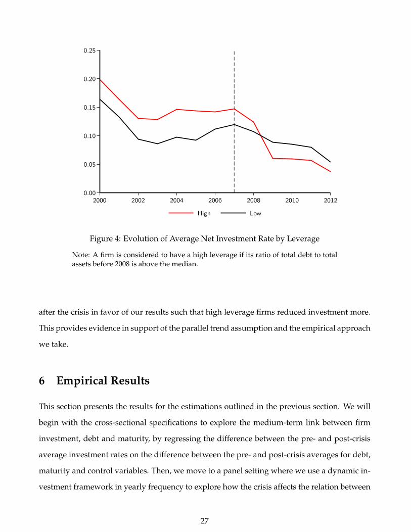
after the shock (i.e., after the crisis starting in 2008). Figure 4 shows the behavior of the average

net investment rate for firms with high and low leverage. A firm is considered to have high

leverage if its leverage before 2008 is above the median of the sample. It is clear that the

investment behavior of these different sets of firms was similar before the crisis but diverged

26

0.00

0.05

0.10

0.15

0.20

0.25

2000 2002 2004 2006 2008 2010 2012

High Low

Figure 4: Evolution of Average Net Investment Rate by Leverage

Note: A firm is considered to have a high leverage if its ratio of total debt to totalassets before 2008 is above the median.

after the crisis in favor of our results such that high leverage firms reduced investment more.

This provides evidence in support of the parallel trend assumption and the empirical approach

we take.

6 Empirical Results

This section presents the results for the estimations outlined in the previous section. We will

begin with the cross-sectional specifications to explore the medium-term link between firm

investment, debt and maturity, by regressing the difference between the pre- and post-crisis

average investment rates on the difference between the pre- and post-crisis averages for debt,

maturity and control variables. Then, we move to a panel setting where we use a dynamic in-

vestment framework in yearly frequency to explore how the crisis affects the relation between

27

investment, debt and maturity. Then we will use the role of weak bank balance sheets from

exposures to sovereign bond holdings as a supply-side shock to investment and as a channel

of rollover risk during the crisis. We end this section with inference of the aggregate effects on

investment of the firm financial frictions explored in this paper.

6.1 Debt Overhang and Rollover Risk

In this section we describe the results of estimating the cross-sectional first-difference equation

2. Table 3 shows our benchmark results where we include our main variables of interest—

leverage, interest coverage, and debt maturity—one-at-a-time to investigate the impact of each

of these three variables. All regressions include four-digit sector-country fixed effects to absorb

demand effects. All variables are expressed in differences, resulting in a fully balanced panel of

firms, equivalent to including firm-fixed effects on the same variables in levels. The differences

are computed as the difference for each firm-level variable between its average over the crisis

period (2008–2012) and its average over the pre-crisis period (2000–2007).

The objective of these regressions is to gain a medium-term perspective on the effects of

financial frictions on firm investment, since the build-up of financial imbalances takes some

time to build, as well as on the de-leveraging process. Moreover by focusing on averages of

investment rates over subperiods we also smooth out any lumpiness in investments within

subperiods. The alternative is to identify the effect we are interested in from year-to-year

changes in the variables of interest, as we will do next.

The results in Column 1 of Table 3 indicate that firms that ended up with higher indebt-

edness (leverage) had on average a significantly lower investment rate as compared to the

pre-crisis period. The same holds for an increase in the associated debt service burden, as cap-

tured by the ratio of interest expenses to EBITDA, as seen in Column 2. Taken together, these

results point to significant debt overhang. An increase in debt maturity between the pre- and

post-crisis periods, however, is associated with higher investment, as seen in Column 3. This

means that firms with longer maturity debt had relatively higher investment rates during the

crisis (i.e., decreased investment less). This result points to increased rollover risk during the

28

Table 3: Debt Overhang, Rollover Risk, and Investment

Dependent variable: ∆ Net investment / Capital

(1) (2) (3) (4)

∆ Debt/Assets −0.0569∗∗∗ −0.0701∗∗∗

(0.0060) (0.0070)∆ Int. Paid/EBITDA −0.0161∗∗∗ −0.0174∗∗∗

(0.0031) (0.0031)∆ Maturity 0.0563∗∗∗ 0.0798∗∗∗

(0.0069) (0.0078)∆ Cash Flow −0.1443∗∗∗ −0.1274∗∗∗ −0.1041∗∗∗ −0.1639∗∗∗

(0.0178) (0.0179) (0.0166) (0.0193)∆ Sales growth 0.2963∗∗∗ 0.2921∗∗∗ 0.2942∗∗∗ 0.2954∗∗∗

(0.0164) (0.0169) (0.0163) (0.0169)∆ Size 0.0308∗∗∗ 0.0345∗∗∗ 0.0287∗∗∗ 0.0294∗∗∗

(0.0037) (0.0048) (0.0038) (0.0039)

Sector-Country FE Yes Yes Yes Yes

Observations 377,576 340,054 377,550 340,002R2 0.06 0.06 0.06 0.06

Standard errors are in parentheses, clustered at the sector-country level.All variables are expressed in differences between their pre-2008 firm-specific mean and their

firm-specific mean over the period 2008–2012. Debt/Assets is total debt scaled by total assets.Interest paid is scaled by EBITDA, ratio that corresponds to the coverage ratio. Maturity is theratio of long-term debt to total debt. Sales is the change in logarithm of sales. Size is measuredby the logarithm of total assets. Cash flow is scaled by total assets.∗p < 0.10, ∗∗p < 0.05, ∗∗∗p < 0.01.

crisis associated with the accumulation of short-term debt during the boom period, which had

to be rolled over at more restrictive conditions during the crisis.

Turning to the control variables, we find that sales growth enters positively, as expected,

signifying the positive effect of growth opportunities on firm investment. Firm size enters

positively, as expected, capturing the presence of increasing returns to scale in investment

and/or the fact that small firms tend to be more affected by financial shocks. Cash flow enters

with a negative sign, showing that firms who hoarded cash during the crisis invested less.

Our results are economically significant. Based on the estimates in Table 3), a one standard-

deviation increase in the debt variable—capturing worsening debt overhang—implies a de-

crease in the investment rate equivalent to 23% of its average change.11 Similarly, a decrease

of one standard deviation in maturity explains about 26% of the average change in the invest-

11This economic effect is computed as follows: we first obtain the standard deviation of the variable of interestfor the sample being used in the estimation; then we calculate the product of the coefficient (shown in Table 3)of a given independent variable with its standard deviation; then we produce the economic effect by dividingthis number by the absolute value of the mean of the left-hand-side variable, since we are interested in scalingthe effects. This produces an estimate of the effect of a standard-deviation change in the value of an independentvariable on the average value of the dependent variable.

29

ment rate.

Table 4 presents the panel regressions with annual frequency. Column 2 of this table in-

cludes interactions with the Post crisis dummy. All other explanatory variables are lagged

one period to mitigate simultaneity bias. The results are consistent with the results obtained

in Table 3. Moreover, we can now interpret the positive coefficient on the Maturity variable

obtained in the cross-sectional regressions, where all variables are included in first-differences.

The level effect of this variable in the panel regression is negative, suggesting that more long-

term debt is affecting investment negatively, consistent with debt overhang. The coefficient on

the interaction between the Post and Maturity variables, however, flips sign, turning positive

during the crisis, consistent with an increase in rollover risk during the crisis period.

The results are economically significant and broadly similar to those obtained using cross-

sectional regressions. Based on the estimates in column 2 of Table 4, a one standard deviation

increase in leverage implies a relative decline in the investment rate during the crisis equiva-

lent to 17% of its average level. Similarly, a one standard deviation decrease in maturity im-

plies a relative decline in the investment rate during the crisis equivalent to 11% of its average

level.

Next, we want to understand what drives these changes from regular to crisis times. There-

fore, we investigate the role of bank-sovereign linkages as potential drivers of these changes.

But before turning to this, we first consider the direct effect of bank weaknesses on investment,

also to make sure that the effects found so far are not contaminated by supply side effects aris-

ing from weak balance sheets.

30

Table 4: Rollover Risk During the Crisis

Dependent variable: Net investment / Capital

(1) (2)

Debt/Assetst−1 −0.0952∗∗∗ −0.0704∗∗∗

(0.0028) (0.0034)Int. Paid/EBITDAt−1 −0.0116∗∗∗ −0.0194∗∗∗

(0.0009) (0.0014)Maturityt−1 −0.2525∗∗∗ −0.2705∗∗∗

(0.0023) (0.0030)Cash flowt−1 0.1683∗∗∗ 0.1842∗∗∗

(0.0047) (0.0064)Sales growtht−1 0.0628∗∗∗ 0.0568∗∗∗

(0.0012) (0.0017)Sizet−1 −0.2248∗∗∗ −0.2286∗∗∗

(0.0013) (0.0014)Postt×Debt/Assetst−1 −0.0440∗∗∗

(0.0030)Postt×Int. Paid/EBITDAt−1 0.0138∗∗∗

(0.0017)Postt×Maturityt−1 0.0298∗∗∗

(0.0031)Postt×Cash flowt−1 −0.0293∗∗∗

(0.0078)Postt×Sales growtht−1 0.0116∗∗∗

(0.0023)Postt×Sizet−1 0.0068∗∗∗

(0.0005)

Firm FE Yes YesSector-Country FE Yes YesBank FE No No

Observations 3,722,889 3,722,889R2 0.20 0.20

Standard errors are in parentheses, clustered at the firm-level. Post is adummy taking the value of 1 starting in 2008 and 0 otherwise. Debt/Assetsis total debt scaled by total assets. Interest paid is scaled by EBITDA, ratiothat corresponds to the coverage ratio. Maturity is the ratio of long-termdebt to total debt. Sales is the change in logarithm of sales. Size is measuredby the logarithm of total assets. Cash flow is scaled by total assets.∗p < 0.10, ∗∗p < 0.05, ∗∗∗p < 0.01.

6.2 The Role of Weak Banks

Table 5 runs multivariate regressions similar to those in Table 3 with the difference that we

now include a Weak bank variable. Each column uses a different definition of the Weak Bank

variable, based on the main bank’s exposure to total sovereign holdings, domestic sovereign

holdings, and periphery country sovereign holdings, respectively. Periphery countries include

31

Greece, Ireland, Italy, Portugal, and Spain.

Table 5: The Role of Weak Banks(Alternative Sovereign Exposures)

Dependent variable: ∆ Net investment / Capital

(1) (2) (3)

∆ All Sovereign ∆ Own Sovereign ∆ Own Sovereign(Periphery)

∆ Debt/Assets −0.0559∗∗∗ −0.0536∗∗∗ −0.0535∗∗∗

(0.0086) (0.0095) (0.0095)∆ Int. Paid/EBITDA −0.0131∗∗∗ −0.0119∗∗∗ −0.0119∗∗∗

(0.0037) (0.0040) (0.0040)∆ Maturity 0.0531∗∗∗ 0.0575∗∗∗ 0.0575∗∗∗

(0.0081) (0.0083) (0.0083)∆ Weak Bank −0.0670∗ −0.2754∗∗∗ −0.2581∗∗

(0.0358) (0.0992) (0.1075)∆ Cash Flow −0.1793∗∗∗ −0.1770∗∗∗ −0.1769∗∗∗

(0.0230) (0.0238) (0.0238)∆ Sales growth 0.2905∗∗∗ 0.2957∗∗∗ 0.2957∗∗∗

(0.0192) (0.0175) (0.0175)∆ Size 0.0143∗∗∗ 0.0146∗∗∗ 0.0146∗∗∗

(0.0044) (0.0047) (0.0047)

Sector-Country FE Yes Yes Yes

Observations 294,255 226,412 226,412R2 0.07 0.07 0.07

Standard errors are in parentheses, clustered at the sector-country level.All variables are expressed in differences between their pre-2008 firm-specific mean and their firm-

specific mean over 2008–2012 (2009–2012 for the case where weak bank corresponds to own-sovereignbond holdings of the bank). Debt/Assets is total debt scaled by total assets. Interest paid is scaled byEBITDA, ratio that corresponds to the coverage ratio. Maturity is the ratio of long-term debt to total debt.Weak Bank measures the exposure of the firm’s main bank to sovereign bonds, scaled by total assets.In column 1, it includes all sovereign bond holdings; in column 2, it includes only own-sovereign bondholdings (domestic sovereign bonds); and lastly, in column 3, it includes own-sovereign bond holdings ifthe parent bank of the firm’s main bank (or the main bank itself in case it does not have a parent bank) islocated in a Periphery country (Periphery domestic sovereign bonds), and otherwise it is set equal to 0.Sales growth is the change in logarithm of sales. Size is measured by the logarithm of total assets. Cashflow is scaled by total assets.∗p < 0.10, ∗∗p < 0.05, ∗∗∗p < 0.01.

The Weak bank variable enters negatively and statistically significant, indicating that there

is a direct negative effect on investment due to reduced credit supply from weak banks. Re-

sults are qualitatively similar across specifications, although the statistical significance on the

Weak Bank variable increases when using own sovereign bond holdings instead of total bond

holdings. This is to be expected as using own sovereign holdings increases the precision re-

garding the factor that contributes to bank weakness during the European sovereign debt crisis

(i.e., sovereign exposure). Importantly, controlling for Weak banks does not alter the results on

our main variables of interest: Debt/Assets and Maturity. The coefficients and statistical sig-

32

nificance of both variables are hardly affected when including the Weak bank variables. Taken

together these results indicate that debt overhang becomes a drag on investment during the

crisis when rollover risk associated with short term debt surfaces. In addition, investment is

depressed during the crisis period because of a weakening of bank balance sheets on account

of sovereign debt exposures.

Next we run a panel difference-in-difference specification that includes triple interactions,

where we interact all firm-specific variables with the Post crisis dummy and the Weak Bank

variables. This specification compares firm investment before and after the crisis as a function

of the debt overhang and rollover risk variables, differentiating between firms that are linked

to weak banks and those that are not. As before, we measure bank weakness using three alter-

native measures of sovereign exposure. First, we measure bank weakness as total sovereign

bond-holdings over total assets of the firm’s main bank. Second, we define bank weakness as

its exposure to domestic sovereign bond holdings scaled by total assets. Using data on do-

mestic holdings has the advantage that one can more accurately measure exposure to weak

sovereigns, though this comes at the cost of a reduced sample size due to data availability.

Third, we refine our measure of bank weakness even further, by setting the exposure to do-

mestic sovereign debt to zero for those banks whose parent entity resides in a non-periphery

euro-area country. In principle, periphery sovereign bonds were the ones subject to the high-

est stress during the crisis, and hence the condition of banks holding these bonds should have

been affected the most. All regressions include firm fixed effects, bank fixed effects, and four-

digit sector-country-year effects. The sample period covers the years 2000 to 2012 and the Post

crisis dummy variable takes on a value of one starting in the year 2008. The bottom panel

reports the estimated total effects of our key variables: leverage, debt service, maturity and

weak bank. The results are presented in Table 6.

33

Table 6: The Role of Weak Banks During the Crisis(Alternative Sovereign Exposures)

Dependent variable: Net investmentt / Capitalt−1

(1) (2) (3)

All Sovereign Own Sovereign Own Sovereign(Periphery)

Interaction effects:†

Postt×Weak Bankt−1× Debt/Assetst−1 −0.4383∗∗∗ −0.9515∗∗∗ −1.1088∗∗∗

(0.0905) (0.2902) (0.2680)Postt×Weak Bankt−1× Int. Paid/EBITDAt−1 0.0404 0.159 0.1654

(0.0557) (0.1734) (0.1642)Postt×Weak Bankt−1×Maturityt−1 −0.1104 0.5232∗∗ 0.9303∗∗∗

(0.0765) (0.2512) (0.2416)Postt×Weak Bankt−1× Cash Flowt−1 −0.0201 −1.3726 −1.2479

(0.2791) (0.8645) (0.7884)Postt×Weak Bankt−1× Sales growtht−1 0.1980∗∗∗ 0.5248∗∗ 0.4543∗∗

(0.0746) (0.2410) (0.2268)Postt×Weak Bankt−1× Sizet−1 −0.0142 0.0038 0.0337

(0.0138) (0.0492) (0.0459)

Total effects:‡

Debt/Assetst−1 −0.1165∗∗∗ −0.0920∗∗∗ −0.0921∗∗∗

(0.0052) (0.0070) (0.0070)Int. Paid/EBITDAt−1 −0.0072∗∗∗ −0.0046∗∗∗ −0.0047∗∗∗

(0.0012) (0.0015) (0.0015)Maturityt−1 −0.2404∗∗∗ −0.2229∗∗∗ −0.2235∗∗∗

(0.0034) (0.0046) (0.0046)Weak Bankt−1 0.0364 0.0609 0.0603

(0.0231) (0.0500) (0.0504)

Firm FE Yes Yes YesSector-Country-Year FE Yes Yes YesBank FE Yes Yes Yes

Observations 2,135,137 1,315,060 1,315,060R2 0.32 0.34 0.34

† Value of the coefficient of the corresponding triple interaction.‡ Total effects of a variable are calculated as the sum of all coefficients where the variable is present using the mean value of thecorresponding weak-banker variable.Standard errors are in parentheses, clustered at the firm-level if no banker fixed effect is included and at firm-bank-level otherwise.

Post is a dummy variable equal 1 starting 2008 (2009 in the case of domestic sovereign bonds, due to data availability). Debt/Assetsis the ratio of total debt to total assets. Interest paid is scaled by EBITDA, ratio that corresponds to the coverage ratio. Maturity isthe ratio of long-term debt to total debt. In Column 1, Weak Bank is measured as the exposure to all sovereign bonds of the firm’smain bank, scaled by the bank’s total assets. In Column 2, Weak Bank is measured as the exposure to domestic sovereign bonds ofthe firm’s main bank, scaled by the bank’s total assets. In Column 3, Weak Bank is measured as the exposure to domestic sovereignbonds of the firm’s main bank, scaled by the bank’s total assets, and is set to zero if the parent bank of the firm’s main bank is notlocated in a Periphery country (i.e., Greece, Ireland, Italy, Portugal and Spain). Sales is the change in logarithm of sales. Size ismeasured by the logarithm of total assets. Cash flow is scaled by total assets.∗p < 0.10, ∗∗p < 0.05, ∗∗∗p < 0.01.

We find that firms with high leverage reduced their investment rates disproportionately

during the crisis when their main bank has a large exposure to sovereign debt. The differential

34

effect of debt service and debt maturity are both insignificant when using total sovereign bond

holdings to measure bank weakness (column 1). However, when measuring sovereign expo-

sure more precisely using domestic sovereign holdings (column 2) we obtain a differential

effect of debt maturity: a higher share of long-term debt is associated with higher net invest-

ment rates during the crisis for firms linked to weak banks, relative to firms whose banks are

not weak. These results imply that the rollover risk associated with short term debt during

the crisis is more pronounced for firms linked to weak banks. In other words, the rollover risk

we identify in part operates through sovereign-bank linkages. Another implication of these

results is that loan evergreening by weak banks to firms facing higher rollover risk played a

limited role during the crisis as these firms decreased investment more.

We obtain very similar results when measuring bank weakness using the domestic sovereign

holdings of periphery country banks only (column 3). In this case we set the exposure to do-

mestic sovereign debt to zero for those banks whose parent entity resides in a non-periphery

euro area country. In principle, periphery sovereign bonds were the ones subject to the largest

decline in value during the crisis, and hence the condition of banks holding these bonds de-

clined the most, ceteris paribus. This implies that the results are largely explained by exposure

to periphery sovereigns. This provides further evidence in support of our hypothesis that the

debt overhang and rollover risk effects are in part driven by increases in sovereign risk trans-

mitted to firms through firm-bank linkages, and that these effects modify firm investment in

comparison to periods of normal market functioning. In the next section we assess the quanti-

tative role of these various effects and their aggregate implications for investment in the euro

area.

6.3 Aggregate Implications

Our results imply that debt overhang and rollover risk negatively affected firm investment

during the crisis. But how much of the decline in aggregate corporate investment since the

onset of the crisis is due to debt overhang and rollover risk? Inferring aggregate effects from

micro-level evidence faces two challenges: external validity and general equilibrium consid-

35

erations. External validity refers to the representativeness of the sample relative to firms in

the economy. Since our data has extensive coverage and is representative of the official data

from Eurostat, the external validity criterion is satisfied and we can use a back of the enve-

lope calculation to link our micro estimates to the actually observed macro level decline in

investment. Such aggregation of micro-level evidence abstracts from any general equilibrium

effects, including the impact of the crisis on the investment demand of unconstrained firms

that do not face debt overhang and rollover risk, such as those arising from a fall in aggregate

demand.

According to official macroeconomic statistics from Eurostat, the average net investment

rate (net investment over GDP) of the non-financial corporate sector in the Euro area fell by 60

percent during the crisis period compared to its pre crisis average level (see Figure 1). Since

our estimates are predicting the decline in investment over capital for the average firm, i,

(∆Ki/Ki), we compare our predictions to the decline in aggregate gross fixed capital formation

for business investment (∆K/K), which is 20 percentage points. Using the estimates from

column (3) of Table 6, we calculate the total effects of each of our variables, leverage, debt

service, and maturity, for the average value of the Weak Bank variable. Next we calculate the

predicted total effects for a one standard deviation change in each of our variables, which are

3, 0.1, and 9 percentage points respectively. Thus, the sum of the predicted percentage point

changes is 12 percentage points. As a result, our coefficients can explain 60 percent of the

20 percentage point decline in aggregate investment (measured as the change in gross fixed

capital formation), with the remainder due to a combination of aggregate demand shocks and

other factors.

7 Conclusions

We quantify the role of financial factors that have contributed to sluggish investment in Eu-

rope in the aftermath of the 2008–2009 crisis. We use a very large pan-European firm-bank-

time level dataset, in which we match the firms to their banks based on banking relation-

ships in 8 countries over time. Our identification relies on a difference-in-difference estima-

36

tion approach, where we compare the investment of high debt (maturity) firms with low debt

(maturity) firms between crisis and normal times, while absorbing demand shocks through

country-four-digit industry-year fixed effects. Furthermore, we use confidential ECB data on

the exposures of banks to (own) sovereign debt together with information on the main bank

relation of each firm to identify the role of sovereign-bank linkages in driving the effect of debt

overhang and rollover risk. Regressions also include bank fixed effects alongside firm fixed

effects to abstract from any unobserved bank and firm characteristics.

Our results highlight the important interaction between the role of firm leverage, debt ma-

turity, and weak bank balance sheets in determining firm investment. Firms with higher lever-

age reduce investment more and this effect strengthens when these firms are linked to weak

banks. Firms that borrowed more short-term suffer from rollover risk and decrease investment

more, and again this effect gets stronger when these firms are connected to weak banks. This

is in sharp contrast to normal times when firms that borrow more short-term tend to invest

more. The effect of bank weakness is strongest for banks in peripheral countries with large ex-

posures to sovereign risk through their holdings of own sovereign debt. In quantitative terms,

the debt overhang and rollover risk channels are both important channels. A simple back

of the envelope calculation based on our firm-level estimates suggests that the debt overhang

and rollover risk channels explain about 60 percent of the actual decline in aggregate corporate

investment during the crisis.

These results highlight that debt overhang and rollover risk of firms, compounded by an

impaired bank lending channel, played a significant role in holding back corporate invest-

ment during the European debt crisis. This is different from (and complementary to) existing

explanations in the literature that have focused on aggregate demand, banking health, and

sovereign-bank linkages to explain the severity of the crisis. These new findings suggest that

growth-enhancing policies that more directly target the financial conditions of firms may be

needed to reduce the debt overhang and stimulate the real economy. The results also point to

the dangers of an overreliance on short-term debt to finance investment during good times.

37

References

Acharya, Viral and Sascha Steffen, “The ‘Greatest’ Carry Trade Ever: Understanding Euro-zone Bank Risks,” Journal of Financial Economics, 2015, 115 (2), 215–236.

, Douglas Gale, and Tanju Yorulmazer, “Rollover risk and market freezes,” The Journal ofFinance, 2011, 66 (4), 1177–1209.

, Itamar Drechsler, and Philipp Schnabl, “A Pyrrhic Victory? Bank Bailouts and SovereignCredit Risk,” Journal of Finance, 2014, 69 (6), 2689–2739.

, Tim Eisert, Christian Eufinger, and Christian Hirsch, “Real Effects of the Sovereign DebtCrisis in Europe: Evidence from Syndicated Loans,” Mimeo, NYU Stern 2014.

Aguiar, Mark, Manuel Amador, and Gita Gopinath, “Investment Cycles and Sovereign DebtOverhang,” Review of Economic Studies, 2009, 76 (1), 1–31.

Altavilla, Carlo, Marco Pagano, and Saverio Simonelli, “Bank Exposures and SovereignStress Transmission,” Review of Finance, 2017, 21 (6), 2103–2139.

Amiti, Mary and David E. Weinstein, “How Much Do Idiosyncratic Bank Shocks Affect In-vestment? Evidence from Matched Bank-Firm Loan Data,” Journal of Political Economy, 2018,126 (2), 525–587.

Becker, Bo and Victoria Ivashina, “Financial Repression in the European Sovereign Debt Cri-sis,” Review of Finance, 2018, 22 (1), 83–115.

Bernanke, Ben, “The Real Effects of the Financial Crisis,” Brookings Papers on Economic Activity,2018, Fall 2018.

Bloom, Nick, Stephen Bond, and John Van Reenen, “Uncertainty and Investment Dynam-ics,” Review of Economic Studies, 2007, 74 (2), 391–415.

Bond, Stephen and Costas Meghir, “Dynamic Investment Models and the Firm’s FinancialPolicy,” The Review of Economic Studies, 1994, 61 (2), 197–222.

Bulow, Jeremy and Kenneth Rogoff, “Sovereign Debt Repurchases: No Cure for Overhang,”The Quarterly Journal of Economics, 1991, 106 (4), 1219–1235.

Caballero, Ricardo J., Takeo Hoshi, and Anil K. Kashyap, “Zombie Lending and DepressedRestructuring in Japan,” American Economic Review, 2008, 98 (5), 1943–1977.

Chaterjee, Stayajit and Burcu Eyigungor, “Maturity, Indebtedness, and Default risk,” Ameri-can Economic Review, 2012, 102 (6), 2674–2699.

Chodorow-Reich, Gabriel, “The Employment Effects of Credit Market Disruptions: Firm-level Evidence from the 2008–9 Financial Crisis,” The Quarterly Journal of Economics, 2014,129 (1), 1–59.

Correa, Ricardo, Horacio Sapriza, and Andrei Zlate, “Liquidity Shocks, Dollar FundingCosts, and the Bank Lending Channel During the European Sovereign Crisis,” InternationalFinance Discussion Papers 1059r, Board of Governors of the Federal Reserve System 2013.

38

Darst, R. Matthew and Ehraz Refayet, “A Collateral Theory of Endogenous Debt Maturity,”Working Paper, Board of Governors of the Federal Reserve System 2017.

Diamond, Douglas W., “Debt Maturity Structure and Liquidity Risk,” The Quarterly Journal ofEconomics, 1991, pp. 709–737.

and Zhiguo He, “A Theory of Debt Maturity: The Long and Short of Debt Overhang,” TheJournal of Finance, 2014, 69 (2), 719–762.

Dinlersoz, Emin, Sebnem Kalemli-Ozcan, Henry Hyatt, and Veronika Penciakova, “Lever-age over the Life Cycle and Implications for Firm Growth and Shock Responsiveness,” 2018.NBER WP 25226.

Gennaioli, Nicola, Alberto Martin, and Stefano Rossi, “Banks, Government Bonds, and De-fault: What Do the Data Say?,” Mimeo, Bocconi University and Universitat Pompeu Fabra2013.

, , and , “Sovereign Default, Domestic Banks, and Financial Institutions,” The Journal ofFinance, 2014, 69 (2), 819–866.

Giannetti, Mariassunta and Steven Ongena, ““Lending by Example”: Direct and IndirectEffects of Foreign Banks in Emerging Markets,” Journal of International Economics, 2012, 86(1), 167–180.

Giroud, Xavier and Holger M. Mueller, “Firm Leverage, Consumer Demand, and Employ-ment Losses during the Great Recession,” The Quarterly Journal of Economics, 2017, pp. 271–316.

Gopinath, Gita, Sebnem Kalemli-Özcan, Loukas Karabarbounis, and Carolina Villegas-Sánchez, “Capital Allocation and Productivity in Southern Europe,” Quarterly Journal ofEconomics, 2017, 132 (4), 1915–1967.

Hart, Oliver and John Moore, “A Theory of Debt Based on the Inalienability of Human Capi-tal,” The Quarterly Journal of Economics, 1994, 109 (4), 841–879.

and , “Debt and Seniority: An Analysis of the Role of Hard Claims in Constraining Man-agement,” The American Economic Review, 1995, pp. 567–585.

and , “Default and Renegotiation: A Dynamic Model of Debt,” The Quarterly Journal ofEconomics, 1998, 113 (1), 1–41.

Hennessy, Christopher A., “Tobin’s Q, Debt Overhang, and Investment,” The Journal of Fi-nance, 2004, 59 (4), 1717–1742.

, Amnon Levy, and Toni M. Whited, “Testing ‘Q’ Theory With Financing Frictions,” Journalof Financial Economics, 2007, 83 (3), 691–717.

Hoshi, Takeo, Anil Kashyap, and David Scharfstein, “The Role of Banks in Reducing theCosts of Financial Distress in Japan,” Journal of Financial Economics, 1990, 27 (1), 67–88.

39

Kalemli-Ozcan, Sebnem, Bent E. Sørensen, Carolina Villegas-Sanchez, Vadym Volosovych,and Sevcan Yesiltas, “How to Construct Nationally Representative Firm Level data fromthe ORBIS Global Database and an Application to Industry Concentration,” September 2015,(21558).

Kashyap, Anil K., Jeremy C. Stein, and David W. Wilcox, “Monetary Policy and Credit Con-ditions: Evidence from the Composition of External Finance,” American Economic Review,1993, 83 (1), 79–98.

, Owen A. Lamont, and Jeremy C. Stein, “Credit Conditions and the Cyclical Behavior ofInventories,” The Quarterly Journal of Economics, 1994, 109 (3), 565–92.

Kashyap, Anil, Owen Lamont, and Jeremy C. Stein, “Monetary Policy and Bank Lending,”in Gregory Mankiw, ed., Monetary Policy, Vol. 29 of Studies in Business Cycles, The Universityof Chicago Press, 1994, chapter 7, pp. 221–261.

Krugman, Paul, “Financing vs. Forgiving a Debt Overhang,” Journal of Development Economics,1988, 29 (3), 253–268.

Laeven, Luc and Fabián Valencia, “Systemic banking crises database,” IMF Economic Review,2013, 61 (2), 225–270.

Lamont, Owen, “Corporate-Debt Overhang and Macroeconomic Expectations,” American Eco-nomic Review, 1995, 85 (5), 1106–17.

Lang, Larry, Eli Ofek, and René M. Stulz, “Leverage, Investment, and Firm Growth,” Journalof Financial Economics, 1996, 40 (1), 3–29.

Miao, Jianjun, “Optimal Capital Structure and Industry Dynamics,” The Journal of Finance,December 2005, 60 (6), 2621–2659.

Myers, Stewart C., “Determinants of Corporate Borrowing,” Journal of Financial Economics,1977, 5 (2), 147–175.

Ongena, Steven, Alexander A Popov, and Neeltje Van Horen, “The Invisible Hand of theGovernment: ’Moral Suasion’ during the European Sovereign Debt Crisis,” Working Paper2017.

Ottonello, Pablo and Thomas Winberry, “Financial Heterogeneity and the Investment Chan-nel of Monetary Policy,” Working Paper 24221, National Bureau of Economic Research 2018.

Peek, Joe and Eric S. Rosengren, “Collateral damage: Effects of the Japanese bank crisis onreal activity in the United States,” American Economic Review, 2000, pp. 30–45.

and , “Unnatural selection: Perverse incentives and the misallocation of credit in Japan,”The American Economic Review, 2005, 95 (4), 1144–1166.

Popov, Alexander and Neeltje Van Horen, “Exporting Sovereign Stress: Evidence From Syn-dicated Bank Lending During the Euro Area Sovereign Debt Crisis,” Review of Finance, 2015,19 (5), 1825–1866.

Whited, Toni M., “Debt, Liquidity Constraints, and Corporate Investment: Evidence FromPanel Data,” The Journal of Finance, 1992, 47 (4), 1425–1460.

40