1

Agency Cost of Debt Overhang with Optimal Investment Timing and Size

Michi Nishihara

Graduate School of Economics, Osaka University, Japan

E-mail: nishihara@econ.osaka-u.ac.jp

Sudipto Sarkar

DeGroote School of Business, McMaster University, Canada

E-mail: sarkars@mcmaster.ca

Chuanqian Zhang

Cotsakos College of Business, William Paterson University, U.S.A

E-mail: zhangc4@wpunj.edu

2

Agency Cost of Debt Overhang with Optimal Investment Timing and Size

Abstract

The debt overhang or underinvestment problem (that is, an equity-maximizing levered firm will under-

invest relative to a firm-value-maximizing firm) is well established in the literature. However, numerical

studies have demonstrated that the agency cost of debt overhang is negligible, which might bring into

question the practical relevance of the debt overhang problem in corporate finance. Our study contributes

to the literature by demonstrating that, when the firm is allowed to choose both the timing and the size of

investment (as is usually the case in real life), the agency cost of debt overhang is substantially larger. It is

shown numerically that, in this scenario, the agency cost of debt overhang is no longer negligible. In fact,

when the firm chooses investment size and capacity as well as debt level optimally, agency cost can be

quite large, about 11% in the base case. Thus, in realistic scenarios, the agency cost can be economically

very significant. This illustrates that the debt overhang problem is of significant practical relevance, and

must not be ignored when making corporate investment decisions.

Keywords: Contingent-claim model; Debt overhang; Underinvestment; Investment trigger;

Agency cost.

JEL Classification Codes: G3.

3

1. Introduction

This paper studies the debt overhang problem and the associated agency cost when a firm has the

flexibility to choose both the timing and the size of its investment. This issue has not been examined in

the literature to date, although there is a substantial literature on debt overhang.1 We show that the agency

cost of debt overhang increases with investment flexibility, and for reasonable parameter values it can be

economically very significant, in contrast to earlier studies which reported negligible agency costs. Thus,

the debt overhang problem is of significant practical importance in corporate investment decisions.

The underinvestment or debt overhang problem, first proposed by Myers (1977), has been widely

studied in the literature. A common approach is to use a contingent-claim model where the capacity is

exogenously specified and the firm chooses the investment timing optimally (Chen and Manso, 2014,

Childs, et al., 2005, Hennessy, 2004, Manso, 2008, Mauer and Ott, 2000, Mello and Parsons, 1992,

Pawlina, 2010, Sarkar and Zhang, 2015, Titman and Tsyplakov, 2007, etc). These papers show that

shareholders of a levered firm have an incentive to delay investing in a project financed by equity,

because existing debt holders would benefit from the investment without contributing to the financing; in

other words, the second-best investment trigger will exceed the first-best trigger. This delayed investment

is tantamount to “under-investing” (Childs, et al., 2005, Sarkar and Zhang, 2015).2

However, the existing literature also finds that the agency cost of debt overhang is very small,3

e.g., Mello and Parsons (1992) estimate it at only 0.8% of firm value. In fact, Parrino and Weisbach

(1999) demonstrate, using Monte Carlo simulations, that agency costs are unlikely to be important in

corporate investment decisions. This leads to the question: if the agency cost of debt overhang is so small,

1 Existing papers allow the firm to choose either the investment timing or the capacity, but not both (see the

following paragraph). 2 In addition, two papers have examined the firm’s investment decision when the timing is exogenously specified.

Jou and Lee (2004) and Moyen (2007) show that shareholders of such a firm will choose a smaller investment size,

or second-best capacity is smaller than first-best, which also depicts underinvestment. 3 Agency cost is the cost imposed on shareholders by the underinvestment incentive, and is given by the margin by

which firm value could have been increased by following the first-best rather than second-best investment policy.

This is a measure of the severity of the debt overhang problem (Mauer and Ott, 2000, Moyen, 2007, Pawlina, 2010).

4

does the debt overhang problem have a material effect on shareholder well-being, or can it, for practical

purposes, be ignored in corporate decisions?

We extend the existing literature to study the investment decision of a levered firm that can

choose both investment timing and investment size, using a “lumpy investment” capacity model similar to

Bar-Ilan and Strange (1999) and Dangl (1999). While this has not been examined yet in the literature, it

should be of significant practical interest, since a firm making a lumpy investment generally gets to

choose both the timing and the scale of the investment (Bar-Ilan and Strange, 1999).

It is not clear how the debt overhang problem will be affected by the ability of the company to

choose investment size. The second-best trigger might be higher than the first-best, but then the second-

best capacity would also exceed the first-best, if chosen optimally (as shown by Bar-Ilan and Strange,

1999, if the firm invests later it will optimally choose a larger capacity). These offsetting effects make it

difficult to determine the overall effect on investment; a higher trigger or delayed investment denotes

underinvestment, while a larger capacity denotes overinvestment. In order to overcome this difficulty, we

have to look for a composite measure that accounts for both effects (timing and size). Section 3.5

discusses two such measures, the expected present value of the investment and the agency cost of debt

overhang.

Our main results are described below. With limited investment flexibility (when firm can choose

only timing or capacity but not both), underinvestment does exist but the agency cost is extremely small,

consistent with earlier studies. But with additional investment flexibility (when the firm can choose both

timing and capacity), we get the following outcomes. When using the first measure above, the

underinvestment problem might be mitigated or exacerbated depending on the cost of capacity. On the

other hand, investment flexibility always increases the agency cost significantly and thus exacerbates the

underinvestment problem. In general, the agency cost with investment flexibility is economically

significant, hence debt overhang should not be ignored in the investment decision-making process. The

magnitude of agency cost depends on the debt level; with the optimal debt level, the agency cost of

underinvestment is economically very significant (about 11% of firm value in the base case).

5

Although our conclusions are based on numerical results, they are robust to changes in parameter

values; thus, we are confident of the generality of the results. The rest of the paper is organized as

follows. Section 2 summarizes the findings in the existing literature, Section 3 develops the model,

Section 4 illustrates the main results, and Section 5 concludes.

2. Literature

As mentioned above, a large number of studies analyze the debt overhang problem when the investment

size is specified and the firm chooses investment timing optimally. These studies show that the second-

best investment trigger exceeds the first-best trigger, implying delayed investment or underinvestment.

Mauer and Ott (2000) and Mello and Parsons (1992) demonstrate underinvestment but report very small

agency costs. Pawlina (2010) also finds extremely small agency cost (except for the unusual scenario of

negative growth), and shows that debt renegotiation in financial distress exacerbates the debt overhang

problem. Sarkar and Zhang (2015) demonstrate underinvestment, and show that performance-sensitive

debt can mitigate the debt overhang problem.

Two papers (Jou and Lee, 2004, and Moyen, 2007) analyze the other scenario, that is, when

investment timing is specified and the firm chooses investment size (capacity). These papers show that

the second-best capacity is smaller than the first-best capacity (which demonstrates underinvestment) and

also that the agency cost is quite small. However, Moyen (2007) also shows that, while agency cost is

very small for irreversible (i.e., not flexible) investment, it is magnified when the firm can adjust the

investment level every period (flexible investment).

Two things are clear from the existing literature. On one hand, there is a potential problem with

debt overhang, which can result in sub-optimal investment policy. On the other hand, the agency cost of

debt overhang (loss in firm value because of the sub-optimal investment policy) seems very small,

perhaps not even relevant for practical purposes. However, as shown by Moyen (2007), if the firm can

choose its investment level every period, the agency cost will be larger. This leads to the question: what if

the firm does not have the ability to change investment level every period, but has a one-time ability to

6

choose investment size (say, when it makes the investment)? This is generally what happens with lumpy

investment, that is, the firm decides on the capacity at time of investment but future adjustments to

capacity are not possible or are prohibitively expensive (Bar-Ilan and Strange, 1999, Dangl, 1999). In

such a scenario, will the underinvestment problem still exist, and will the agency cost be large enough to

matter for practical purposes? This is the question our paper attempts to answer.

3. The Model

We assume that the levered firm has an investment opportunity, and it can choose the time of investment

(when the size is pre-specified, as in Mauer and Ott, 2000, Sarkar and Zhang, 2015) or the size (when the

timing is pre-specified, as in Jou and Lee, 2004, Moyen, 2007). In addition, we allow the firm to choose

both timing and size of investment, using the “lumpy investment” approach of Bar-Ilan and Strange

(1999).4

3.1. The Investment Project

When the firm decides to invest in the project, it incurs a one-time investment cost of κQη, where Q is the

capacity of the project (i.e., units of output per unit time), Qη is the amount of capital required to produce

at that capacity,5 and κ is the cost per unit of capital. This investment cost function is commonly used in

the literature (Bar-Ilan and Strange, 1999, Bertola and Caballero, 1994, Dangl, 1999). The output price is

$x per unit, and is stochastic, following the usual lognormal process:

dx = μxdx + σxdz (1)

where µ is the expected growth rate and σ is the volatility of the price process, both assumed constant,

and dz is the increment to a standard Brownian Motion Process. We assume that operating costs are zero,

so the firm always operates at full capacity. The firm’s earnings (after interest) are taxed at a constant rate

4 Thus, our results apply to “lumpy” as opposed to “incremental” investment (see Bar-Ilan and Strange, 1999, and

Dangle, 1999, for discussions of lumpy versus incremental investment). In lumpy investment, adjustments to

installed capacity are ruled out because of economic, environmental, physical or other restrictions. 5 Note that we must have η > 1 to ensure decreasing returns to scale, otherwise the optimal capacity will be infinitely

large.

7

of τ, and all cash flows are discounted at a constant discount rate of r. Shareholders receive all residual

cash flows after interest and taxes.

3.2. The Capital Structure

The firm is levered before it makes the investment decision. In some models, the leverage or debt-issue

decision is taken at the same time as, or after, the investment is made (e.g., Leland, 1998); in such cases,

maximizing equity value is tantamount to maximizing firm value, hence the investment decision will

always be first-best and there will be no debt overhang problem. Since we are interested in the spread

between first-best and second-best investment, we assume that the investment decision is made after the

leverage decision has been made and the debt is in place, as in Hirth and Uhrig-Homburh (2010), Mao

(2003), Mauer and Ott (2000), Sarkar and Zhang (2015), Brander and Lewis (1986) and Jou and Lee

(2004). In our model, therefore, a manager looking after shareholder interests will choose an investment

policy (timing and size) that maximizes equity value rather than total firm value, that is, will follow a

second-best investment policy.

With a levered firm we must consider the possibility of bankruptcy. The bankruptcy timing

decision will be made so as to maximize equity value, as is standard in the literature. This means the firm

will declare bankruptcy when x falls to a sufficiently low level (Leland, 1994, Mauer and Ott, 2000, etc).

When the company declares bankruptcy, the equity holders will depart with no payoff and the

bondholders will take over the assets of the firm after incurring bankruptcy costs (that is, the absolute

priority rule will be enforced).

We assume that the magnitude of the fractional bankruptcy cost is α1 prior to investment and α2

after investment, where 1 ≥ α1 ≥ α2 ≥ 0. This is because after investment the firm has tangible assets

(buildings, plant, machinery, etc), while before investment its only asset is the (intangible) option to

invest (Sarkar and Zhang, 2015); since the magnitude of bankruptcy cost is known to be a decreasing

function of asset tangibility (Brealey and Myers, 2000), the post-investment bankruptcy cost should be

smaller than the pre-investment bankruptcy cost.

8

3.3. Valuation

Unlevered Firm

The unlevered firm value or project value will be a function of the state variable x, and will also depend

on whether the option to invest has been exercised. Let the value be U0(x) before investment and U1(x)

after investment (i.e., an operating project). Then it can be shown that:6

1xZ)x(U 00

(2)

)r/(Qx)1()x(U1 (3)

where Z0 is a constant to be determined by boundary conditions (below), and γ1 and γ2 are the positive

and negative solutions, respectively, of the quadratic equation 0r)1(5.0 2 , given by:7

22221 /5.0/r2/5.0 (4)

22222 /5.0/r2/5.0 (5)

To identify the constants, we use the value-matching and smooth-pasting conditions (Dixit and Pindyck,

1994). The former is given by: Q)x(U)x(U i1i0 , and the latter by: )x('U)x('U i1i0 , where xi is

the optimal investment trigger. These boundary conditions give:

)/11)(1(

)r(Qx

1

1

i

and

)r(

xQ)1(Z

1

1

i0

1

.

Levered Firm

Post-investment: It can also be shown that the post-investment debt and equity values are given by:

2xZr/c)x(D 11

(6)

2xZr/c)r/(Qx)1()x(E 21

(7)

6 All derivations are available from authors on request. 7 Note that γ1 > 1 and γ2 < 0.

9

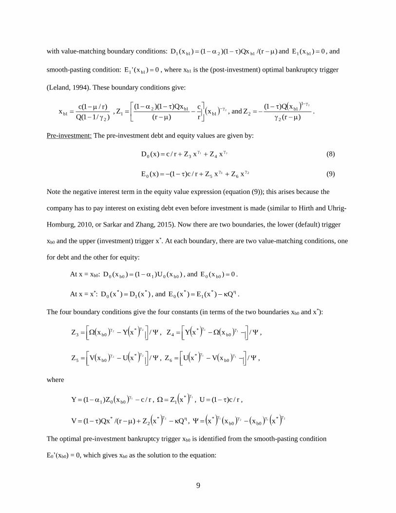
with value-matching boundary conditions: )r/(Qx)1)(1()x(D 1b21b1 and 0)x(E 1b1 , and

smooth-pasting condition: 0)x('E 1b1 , where xb1 is the (post-investment) optimal bankruptcy trigger

(Leland, 1994). These boundary conditions give:

)/11(Q

)r/1(cx

2

1b

, 2

1b1b2

1 xr

c

)r(

Qx)1)(1(Z

, and

)r(

xQ)1(Z

2

1

1b2

2

.

Pre-investment: The pre-investment debt and equity values are given by:

21 xZxZr/c)x(D 430

(8)

21 xZxZr/c)1()x(E 650

(9)

Note the negative interest term in the equity value expression (equation (9)); this arises because the

company has to pay interest on existing debt even before investment is made (similar to Hirth and Uhrig-

Homburg, 2010, or Sarkar and Zhang, 2015). Now there are two boundaries, the lower (default) trigger

xb0 and the upper (investment) trigger x*. At each boundary, there are two value-matching conditions, one

for debt and the other for equity:

At x = xb0: )x(U)1()x(D 0b010b0 , and 0)x(E 0b0 .

At x = x*: )x(D)x(D *1

*0 , and Q)x(E)x(E *

1*

0 .

The four boundary conditions give the four constants (in terms of the two boundaries xb0 and x*):

/xYxZ

22 *

0b3 ,

/xxYZ 1

1

0b*

4 ,

/xUxVZ

22 *

0b5 ,

/xVxUZ 1

1

0b*

6 ,

where

r/cxZ)1(Y 1

0b01

, 1*1 xZ

, r/c)1(U ,

QxZ)r/(Qx)1(V

2*2

* , 212

1 *0b0b

* xxxx

The optimal pre-investment bankruptcy trigger xb0 is identified from the smooth-pasting condition

E0’(xb0) = 0, which gives xb0 as the solution to the equation:

10

0xZxZ 21

0b260b15

(10)

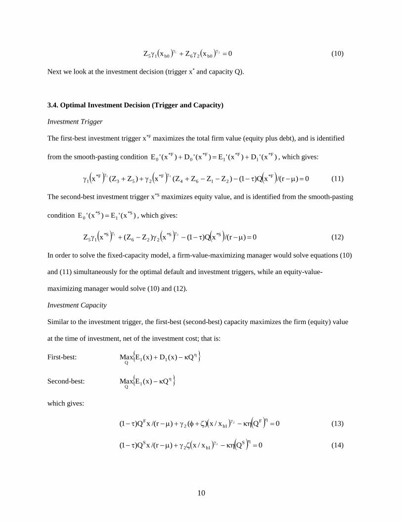
Next we look at the investment decision (trigger x* and capacity Q).

3.4. Optimal Investment Decision (Trigger and Capacity)

Investment Trigger

The first-best investment trigger x*F maximizes the total firm value (equity plus debt), and is identified

from the smooth-pasting condition )x('D)x('E)x('D)x('E F*1

F*1

F*0

F*0 , which gives:

0)r/(xQ)1()ZZZZ(x)ZZ(x F*2164

F*253

F*1

21

(11)

The second-best investment trigger x*S maximizes equity value, and is identified from the smooth-pasting

condition )x('E)x('E S*1

S*0 , which gives:

0)r/(xQ)1(x)ZZ(xZ S*S*226

S*15

21

(12)

In order to solve the fixed-capacity model, a firm-value-maximizing manager would solve equations (10)

and (11) simultaneously for the optimal default and investment triggers, while an equity-value-

maximizing manager would solve (10) and (12).

Investment Capacity

Similar to the investment trigger, the first-best (second-best) capacity maximizes the firm (equity) value

at the time of investment, net of the investment cost; that is:

First-best: Q)x(D)x(EMax 11Q

Second-best: Q)x(EMax 1Q

which gives:

0Qx/x)()r/(xQ)1( F1b2

F 2

(13)

0Qx/x)r/(xQ)1( S1b2

S 2

(14)

11

where x is the state variable when the investment is made, QF (QS) is the first-best (second-best) capacity,

1)/11/()1)(1()r/c( 22 , and )1/()r/c)(1( 2 .

In order to solve the fixed-timing model (with immediate investment, or investment trigger

specified to be x* = x), a firm-value-maximizing manager would solve equations (10) and (13)

simultaneously for the optimal default trigger and capacity, while an equity-value-maximizing manager

would solve (10) and (14).

Finally, in order to solve the model when both investment trigger and capacity can be chosen by

the firm, a firm-value-maximizing manager would solve equations (10), (11) and (13) simultaneously for

the optimal default trigger, investment trigger and capacity, respectively, while an equity-value-

maximizing manager would solve (10), (12) and (14).8

3.5. Underinvestment

We identified above the first-best and second-best investment triggers (x*F and x*S) and first-best and

second-best capacities (QF and QS). In the context of our model, underinvestment would mean x*F < x*S

when Q is fixed, or QF > QS when x* is fixed. However, it is not clear how to characterize under (over)-

investment when both Q and x* are chosen by the firm, because of the following reason. The optimal

capacity is an increasing function of x at the time of investment (Bar-Ilan and Strange, 1999, or Dangle,

1999), thus if we have x*F < x*S it follows that QF < QS. Since the former indicates underinvestment and

the latter indicates overinvestment, it is difficult to compare the first-best and second-best outcomes,

hence it is difficult to say whether there is under- or over-investment. What is needed is a composite

measure that takes into account both aspects of investment (timing and size), and therefore allows us to

make a direct comparison of first-best and second-best outcomes.

We consider two such composite measures. First, since we know that delayed investment is larger

in size, the way to compare first-best and second-best investment is to consider the EPV (expected present

value) of the investment size (in dollars). This will be determined by the investment size, the investment

8 These systems of equations have to be solved numerically because no closed-form solutions are available.

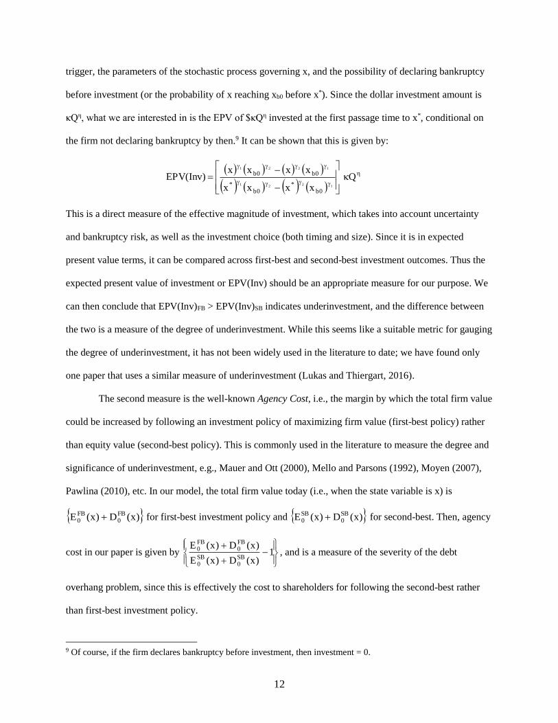
12

trigger, the parameters of the stochastic process governing x, and the possibility of declaring bankruptcy

before investment (or the probability of x reaching xb0 before x*). Since the dollar investment amount is

κQη, what we are interested in is the EPV of $κQη invested at the first passage time to x*, conditional on

the firm not declaring bankruptcy by then.9 It can be shown that this is given by:

Q

xxxx

xxxx)Inv(EPV

12

21

1221

0b*

0b*

0b0b

This is a direct measure of the effective magnitude of investment, which takes into account uncertainty

and bankruptcy risk, as well as the investment choice (both timing and size). Since it is in expected

present value terms, it can be compared across first-best and second-best investment outcomes. Thus the

expected present value of investment or EPV(Inv) should be an appropriate measure for our purpose. We

can then conclude that EPV(Inv)FB > EPV(Inv)SB indicates underinvestment, and the difference between

the two is a measure of the degree of underinvestment. While this seems like a suitable metric for gauging

the degree of underinvestment, it has not been widely used in the literature to date; we have found only

one paper that uses a similar measure of underinvestment (Lukas and Thiergart, 2016).

The second measure is the well-known Agency Cost, i.e., the margin by which the total firm value

could be increased by following an investment policy of maximizing firm value (first-best policy) rather

than equity value (second-best policy). This is commonly used in the literature to measure the degree and

significance of underinvestment, e.g., Mauer and Ott (2000), Mello and Parsons (1992), Moyen (2007),

Pawlina (2010), etc. In our model, the total firm value today (i.e., when the state variable is x) is

)x(D)x(E FB0

FB0 for first-best investment policy and )x(D)x(E SB

0SB0 for second-best. Then, agency

cost in our paper is given by

1

)x(D)x(E

)x(D)x(ESB0

SB0

FB0

FB0 , and is a measure of the severity of the debt

overhang problem, since this is effectively the cost to shareholders for following the second-best rather

than first-best investment policy.

9 Of course, if the firm declares bankruptcy before investment, then investment = 0.

13

4. Results

We first illustrate, for benchmarking purposes, the two instances of underinvestment already discussed in

the existing literature. We demonstrate “delayed investment” (Childs, et al., 2005, Mauer and Ott, 2000,

Sarkar and Zhang, 2015) by showing that, for fixed investment size, an equity-value-maximizing manager

will delay investment relative to a firm-value-maximizing manager; that is, the second-best investment

trigger will exceed the first-best trigger. We also demonstrate capacity underinvestment (Jou and Lee,

2004, Moyen, 2007) by showing that, for fixed investment trigger, the second-best investment size is

smaller than the first-best investment size. Finally, we derive new results, for the case of investment

flexibility, when both investment trigger and investment size can be chosen by the firm. This scenario has

not been examined in the existing literature.

We present results obtained by numerically solving the model of Section 3 (since no analytical

solution exists). For numerical results, we need to specify values of the input parameters. We start with a

set of reasonable “base-case” parameter values, and then repeat the computations with a range of

parameter values, in order to ensure robustness of the results and also to derive the comparative static

relationships.

4.1. Base-case Parameter Values

The parameter values are chosen to be similar to existing contingent-claim studies such as Leland (1994),

Mauer and Ott (2000), Pawlina (2010), etc, wherever possible. Accordingly, we use the following:

discount rate r = 6%, growth rate µ = 1% and volatility σ = 15% and effective tax rate τ = 15%. For the

bankruptcy cost, the existing studies use a range of values. Leland (1994), for instance, uses 50%, but a

number of papers have argued that 50% is too high, and have estimated bankruptcy cost at significantly

lower levels, closer to 25% (Andrade and Kaplan, 1998, Davydenko, et al., 2012, Hackbarth and Mauer,

2012). We therefore set the bankruptcy cost of an active (post-investment) firm at α2 = 25%. Prior to

investment, however, the bankruptcy cost should be significantly higher (as explained in Section 3.2),

14

because the firm’s only asset at that time is the (intangible) option to invest, and intangible assets are

subject to significantly higher bankruptcy costs (Brealey and Myers, 2000). We therefore set the pre-

investment bankruptcy cost at α1 = 50%. For the capacity cost parameters, we use κ = 6 and η = 1.75,

close to Bar-Ilan and Strange (1999). Finally, we choose output price x = 0.8 without loss of generality,

since it is just a scaling variable.

However, while the above “base-case” parameter values are chosen to be realistic, all the

computations are repeated with a wide range of parameter values, in order to ensure the generality and

robustness of our numerical results. We therefore feel confident about the generality of our results, even

in the absence of analytical results.

4.2. Numerical Results

We start with the base-case parameter values specified in Section 4.1: r = 6%, µ = 1%, σ = 15%, τ = 15%,

α1 = 50%, α2 = 25%, κ = 6, η = 1.75 and x = 0.8. First we examine the investment timing decision when

the capacity is fixed at Q = 3. Next we examine the capacity decision when the investment timing is

specified at x* = x = 0.9. Finally we examine the hitherto ignored scenario where both investment timing

and capacity are chosen by the firm. In all cases, we start with a given debt level (c = 0.3) and then repeat

the procedure for various debt levels.

4.2.1. With exogenously-specified capacity (Q = 3)

Solving the model of Section 3 with coupon c = 0.3, we get the following output: first-best investment

trigger x*F = 1.3860 and second-best investment trigger x*S = 1.4048. Since x*S > x*F, this illustrates

underinvestment in the form of delayed investment, consistent with Mauer and Ott (2000), Pawlina

(2010), Sarkar and Zhang (2015), etc.

Next, the expected present value of investment (EPV(Inv) from Section 3.5) is $10.4462 for first-

best and $10.1154 for second-best. This also demonstrates underinvestment, the magnitude of which is

15

(10.4462/10.1154 – 1) = 3.27%. Finally, the total firm value (equity plus debt) is $8.3742 for first-best

and $8.3719 for second-best, giving an agency cost of (8.3742/8.3719 – 1) = 0.03%.

Figure 1 about here

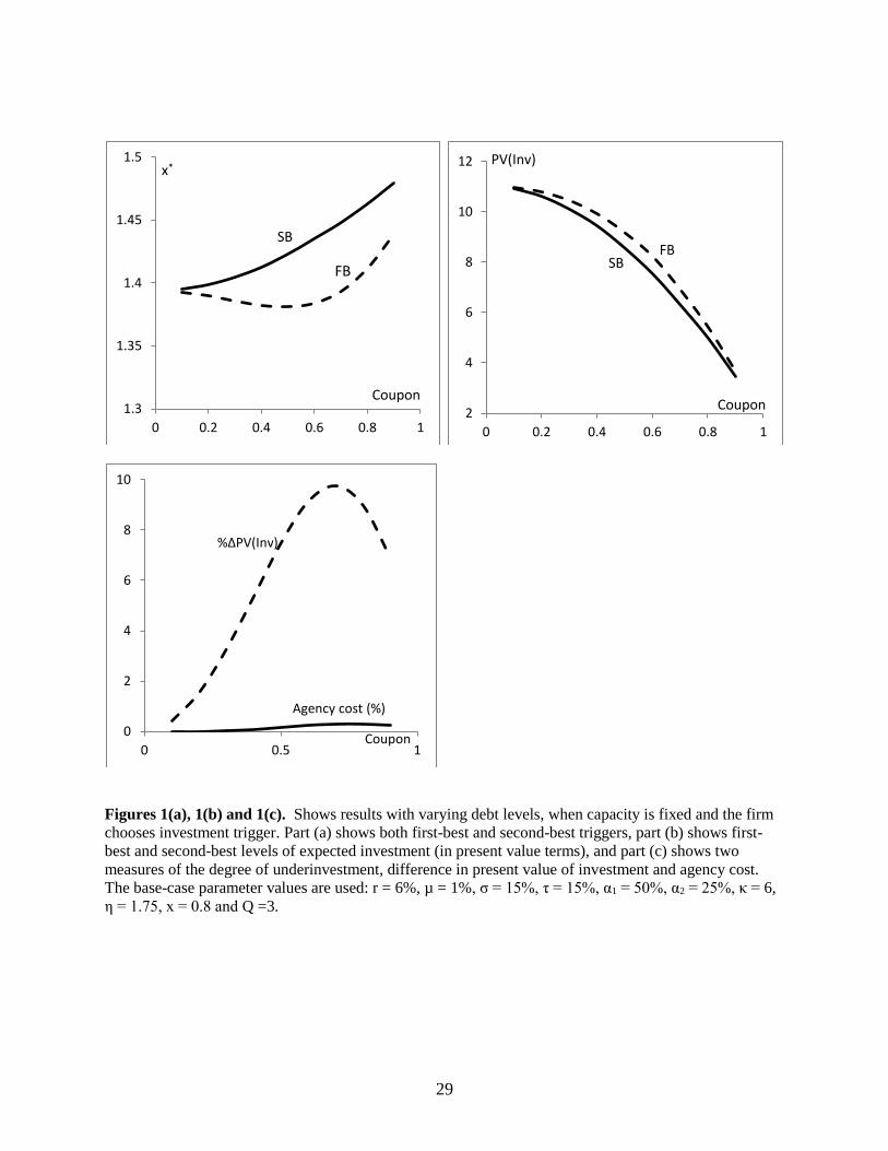
Figure 1 displays the corresponding results with different levels of debt, c. We note from Figure

1(a) that the first-best investment trigger initially falls and then rises as c is increased, while the second-

best trigger is unambiguously increasing in c. We also note that: (i) the latter always exceeds the former,

indicating underinvestment for all debt levels; and (ii) the spread between x*S and x*F first widens and

then narrows as the debt level is increased.

Figure 1(b) compares first-best and second-best investment in terms of the expected present value

of investment. For both first-best and second-best, EPV(Inv) is a monotonically decreasing function of

debt level. However, it can be noted that: (i) the first-best EPV(Inv) always exceeds the second-best,

confirming underinvestment; and (ii) the spread between first-best and second-best is initially increasing

and subsequently decreasing in debt level.

Finally, Figure 1(c) shows the severity of the debt overhang problem, measured by (i) the

difference between first-best and second-best EPV(Inv), and (ii) agency cost. In both cases, the effect of

debt level is non-monotonic; the difference in EPV(Inv) and the agency cost are both initially increasing

and subsequently decreasing in debt level. The former rises from 0.41% to 9.75% and then falls to 6.88%

as the debt level is increased from c = 0.1 to 0.7 and then to 0.9 (corresponding to leverage ratios of 19%,

84% and 95% respectively). The agency cost rises from 0.0005% to 0.30% and then falls to 0.23% as the

debt level is increased from c = 0.1 to 0.8 and then 0.9 (with corresponding leverage ratios of 19%, 90%

and 95% respectively). While the former measure of underinvestment is not negligible, the agency cost is

very small for all debt levels, consistent with earlier papers (Mauer and Ott, 2000, Pawlina, 2010, etc).

It is also clear that the debt overhang or underinvestment effect, measured either way, is initially

an increasing function and subsequently a decreasing function of the debt level. This can be explained as

16

follows. As the amount of debt is increased, there is more wealth that can be transferred from bondholders

to shareholders, hence the agency problem of underinvestment should become more acute (or the

underinvestment incentive should rise). This makes underinvestment an increasing function of debt level.

On the other hand, a higher debt level increases the probability of bankruptcy before investment, which

would leave the shareholder with nothing; this reduces the underinvestment incentive and causes

underinvestment to be a decreasing function of debt level. Because of the two opposing effects, the

overall effect of debt level on underinvestment is non-monotonic. For small debt level, the risk of

bankruptcy is not a serious concern, hence the former effect dominates and the overall effect is that

underinvestment increases with debt level. But when the debt level is already high, there is a significant

probability of bankruptcy before investment, which increases the shareholders’ incentive to invest. Thus,

when the debt level is high, the latter effect dominates, and the degree of underinvestment is a decreasing

function of debt level. The overall result, therefore, is that the degree of underinvestment is initially

increasing and subsequently decreasing in debt level, as shown in Figure 1(c).

4.2.2. With exogenously-specified investment trigger

We repeat the above exercise with the investment trigger specified at x* = x = 0.9 (i.e., investment has to

be made immediately), but capacity can be chosen optimally. Thus, the first-best capacity QF will be

chosen to maximize total firm value, while the second-best capacity QS will maximize equity value. With

the same parameter values, we get QF = 1.6543 and QS = 1.6500. This illustrates underinvestment

(smaller investment size) caused by equity-maximization rather than firm-value-maximization, and is

consistent with Jou and Lee (2004) and Moyen (2007). In terms of investment size in dollars, the

investment is worth $14.4786 (first-best) and $14.4128 (second-best), for a difference of 0.46%. The total

firm value is $11.5706 for first-best and $11.5705 for second-best, resulting in an agency cost that is

negligible (0.001%).

Figure 2 about here

17

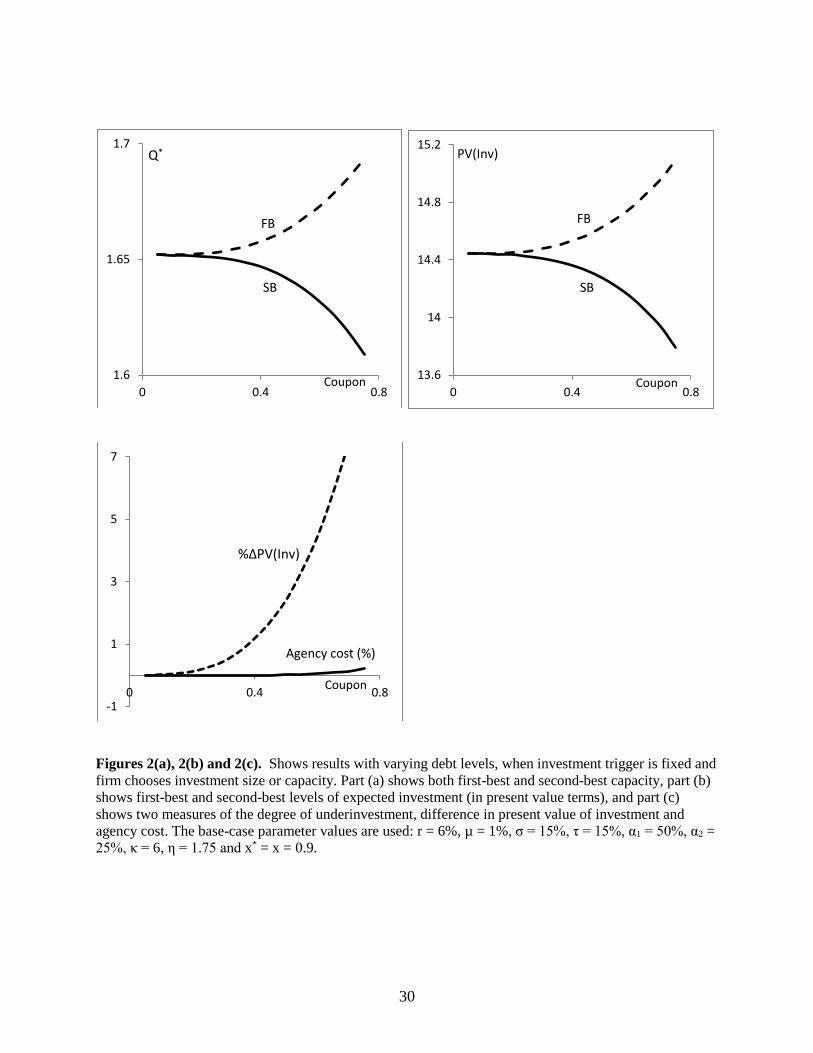
Figure 2 shows the results with varying levels of debt. In Figure 2(a), we note that QF is an

increasing function of coupon c, while QS is a decreasing function. Also, QF exceeds QS in all cases,

demonstrating underinvestment, the degree of which is an increasing function of debt level. The results

are very similar with investment dollar amount (Figure 2(b)). Finally, Figure 2(c) shows the severity of

underinvestment (in two different measures) and how it is affected by the debt level. The degree of

underinvestment, measured by the difference in EPV(Inv), increases from 0 to 9.43% as the debt level is

increased from 0.05 to 0.75 (corresponding to leverage ratio of 7.6% and 97% respectively). But when

underinvestment is measured by agency cost, it rises from 0 to 0.22% for the same increase in debt level.

In both cases, the severity of underinvestment is a monotonically increasing function of the debt

level (in contrast to Section 4.2.1, where it was initially increasing and subsequently decreasing). The

reason for this difference is that in this section the investment takes place right away (since x = x* by

assumption), hence there is no risk of bankruptcy prior to investment; thus the second effect discussed in

Section 4.2.1 does not exist, as a result of which the underinvestment incentive increases with debt levels

for all debt levels.

Thus, this sub-section (when company chooses investment capacity rather than timing) again

demonstrates underinvestment. Also, as in the previous sub-section, it can be noted that the agency cost is

very small in magnitude while the difference in EPV(Inv) can be significant.

4.2.3. Both investment size and trigger chosen by the firm

The above two sections (4.2.1 and 4.2.2) demonstrated the underinvestment phenomenon as well as the

fact that agency cost is very small in magnitude. Both findings verify existing results, but are not new

results. What has not been examined yet is how investment flexibility (when the firm can choose both

timing and capacity) affects the underinvestment problem.

Let us consider the expected present value of investment first. As mentioned earlier, because x*S

> x*F, we will have QS > QF. The latter inequality means that underinvestment will be mitigated, since a

18

larger capacity will be chosen. However, the higher QS will result in higher x*S (which exacerbates

underinvestment), which in turn will result in larger capacity QS (which mitigates underinvestment), and

so on. Because of the two opposing effects (“higher trigger” implying underinvestment and “larger

capacity” implying overinvestment), it is difficult to predict whether the final effect will be to mitigate or

exacerbate the underinvestment problem. Intuitively, it should depend on how expensive the capacity is,

i.e., the value of the parameters κ and η. If κ and η are larger, it will be more expensive to install capacity,

and the “larger capacity” effect will be more subdued, so the net effect is more likely to be greater

underinvestment. Thus, for high capacity costs, underinvestment is likely to be exacerbated by investment

flexibility. Conversely, for lower capacity costs (smaller κ and η) the “larger capacity” effect is more

likely to dominate, hence the net effect is more likely to be mitigation of the underinvestment problem.

Thus, it is not clear whether greater investment flexibility (ability to choose both timing and size) will

mitigate or exacerbate the underinvestment problem, but it is more likely to exacerbate (mitigate) it when

κ and η are large (small). This is confirmed by numerical results in Section 4.2.4.

For the agency cost, the effect of being allowed the additional flexibility to choose capacity will

be as follows. Because the company has the additional flexibility (and in the absence of informational

asymmetry), rational bondholders will expect that shareholders will use the additional investment

flexibility to increase activities that transfer wealth from bondholders to shareholders (such as

underinvestment), thus they will penalize the company to a larger extent (in the form of higher cost of

debt). Shareholders will end up paying the additional cost, as a result of which agency cost will go up.

Therefore, greater investment flexibility should result in a higher agency cost of underinvestment. This is

consistent with Moyen’s (2007) finding; in particular, she mentions (p. 435) “More investment flexibility

magnifies the debt overhang cost.”10 A similar argument was made in the context of the risk-shifting

agency problem by MacKay (2003).

10 In Moyen’s (2007) model, however, the firm can invest in every period and investment flexibility denotes the ease

of reversibility of the investment.

19

To identify the net effect, we solved the model of Section 3 with the firm choosing both

investment timing and capacity simultaneously. With the same base-case parameter values (Section 4.1),

we get the following results:

First-best: x*F = 1.0595, QF = 2.0543, EPV(Inv) = $10.3022, total firm value = $8.9577

Second-best: x*S = 1.3296, QS = 2.7794, EPV(Inv) = $10.0956, total firm value = $8.3958

As expected, second-best investment is delayed relative to first-best (implying underinvestment) but

larger in size than first-best investment (implying overinvestment). To gauge the overall effect, we can

look at the present value of investment, which is smaller for the equity-value-maximizing company; we

therefore conclude that the overall effect is underinvestment.

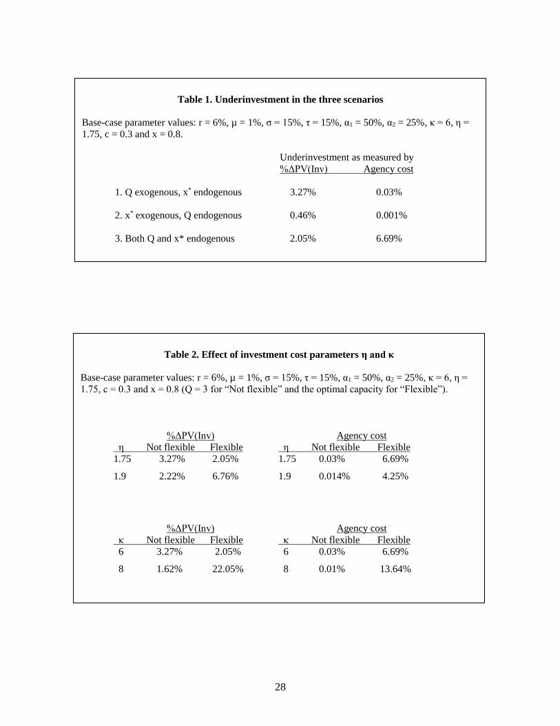
Table 1 about here

Comparing the first-best and second-best outcomes, we find that the difference in EPV(Inv) is

(10.3022/10.0956 – 1) = 2.05%, and the agency cost is (8.9577/8.3958 – 1) = 6.69%. For completeness,

we summarize the results for all three scenarios in Table 1, two with reduced investment flexibility

(choose either timing or size) and the last with increased investment flexibility (choose both timing and

size). We note that the degree of underinvestment measured by the difference in present value of

investment can rise or fall with additional investment flexibility. However, the striking result is that

agency cost of debt overhang is significantly higher as a result of investment flexibility, 6.69% compared

to 0.03% and 0.001% (for the same parameter values).

Figure 3 about here

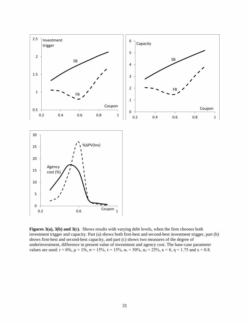
Figure 3 shows the results from optimizing both investment trigger and capacity simultaneously

for varying levels of debt c. Part (a) shows the first-best and second-best investment triggers as functions

of c. It can be noted that the behavior is very similar to that in Figure 1(a); that is, the first-best trigger is

20

initially a decreasing function and subsequently an increasing function of the debt level, while the second-

best trigger is an increasing function of debt level. Moreover, (i) the second-best trigger always exceeds

the first-best trigger, which illustrates underinvestment; and (ii) the spread between the two triggers is

initially increasing and subsequently decreasing in the debt level.

Figure 3(b) shows the first-best and second-best capacity as functions of debt level c. The second-

best capacity QS is an increasing function of debt level while the first-best capacity QF is initially

decreasing and subsequently increasing in debt level. We can note that the behavior is similar to Figure

3(a), which is not surprising since delayed (earlier) investment is strongly associated with larger (smaller)

investment (Bar-Ilan and Strange, 1999). In all cases, we note that QF ≤ QS, which indicates

overinvestment. Also, the difference between the first-best and second-best capacity is initially increasing

and subsequently decreasing in the debt level.

Figure 3(c) shows the severity of underinvestment (measured by difference in EPV(Inv) and

agency cost) as a function of the debt level. The difference in EPV(Inv) rises from 2.05% to 26.7% and

then falls to 0.25% as the debt level is increased from c = 0.3 to 0.6 and then to 0.9 (corresponding to

leverage ratios of 48%, 76% and 94% respectively). Comparing these to Figure 1(c), we can see that it is

not possible to state unambiguously the effect of the added flexibility (from being able to choose the

investment size) on the degree of underinvestment. However, it is clear that, with investment flexibility,

the degree of underinvestment measured this way can be of significant magnitude.

When measured by the agency cost, the degree of underinvestment rises from 6.69% to 17.40%

and then falls to 0.58% as debt level is increased from c = 0.3 to 0.5 and then to 0.9 (corresponding to

leverage ratios of 48%, 68% and 94% respectively). Comparing these outputs to Figure 1(c), it is clear

that the added investment flexibility of being able to choose the capacity results in a significantly higher

agency cost than in the existing literature (which ignores investment flexibility, e.g., Mauer and Ott, 2000,

Mello and Parsons, 1992, Parrino and Weisbach, 1999). Thus, investment flexibility unambiguously

increases the agency cost of debt overhang or underinvestment.

21

Under both measures, the severity of the underinvestment problem is initially an increasing

function and subsequently a decreasing function of debt level. The reason for this non-monotonicity was

discussed in Section 4.2.1.

We summarize the main results below.

Result 1. Looking at investment timing and size, it is not clear whether the underinvestment problem will

survive under investment flexibility (because of the offsetting effects). However, looking at the two

composite measures of underinvestment, it is clear that underinvestment does exist under investment

flexibility.

Result 2. (i) The effect of investment flexibility on the degree of underinvestment measured by the

expected present value of investment can be positive or negative, depending on cost of capacity;

(ii) However, the agency cost of debt overhang always increases with investment flexibility.

Result 3. Earlier studies argued that agency cost is negligibly small, but we find that, with investment

flexibility, agency cost is generally (with reasonable input parameters) economically significant;

therefore, the debt overhang problem should be highly relevant in corporate investment decisions.

Finally, it is clear from Figure 3(c) that the agency cost is very sensitive to the debt level, since

the degree of underinvestment with investment flexibility varies considerably with debt level. Thus, how

large the agency cost is (and consequently, how significant the debt overhang problem might be in

practice) would depend on the debt level used by the firm. This leads to the question: what is the

appropriate level of debt? This issue is discussed in Section 4.3 below.

22

4.2.4. Comparative Static Results

The numerical procedure is repeated with different parameter values to test for the robustness of the main

results. Table 2 summarizes the relevant results; in table 2, “not flexible” means the firm can choose only

the timing (with size specified), and “flexible” means the firm can choose both timing and size.

Table 2 about here

The left half shows the degree of underinvestment in terms of expected present value of investment; from

Section 3.5, this is given by

1

)Inv(EPV

)Inv(EPV

SB

FB . The right half shows the agency cost; from Section 3.5,

this is given by

1

)x(D)x(E

)x(D)x(ESB0

SB0

FB0

FB0 . Table 2 only shows the comparative static results for the

investment cost parameters η and κ. The other parameters are less interesting because the effect of

flexibility on underinvestment does not change from the base-case results, hence these are not reported.

The results are consistent with the discussion in Section 4.2.3. In all cases the agency cost is

higher with investment flexibility (when the firm chooses both timing and size of investment). While

agency cost is negligible under “not flexible,” it is quite large under “flexible,” e.g., 6.69% for the base-

case parameter values.

For the expected present value of investment, however, the effect of investment flexibility is

ambiguous. The effect depends on the investment cost parameters η and κ. For η = 1.75, the degree of

underinvestment is 3.27% for non-flexible and falls to 2.05% for flexible investment. However, when

capacity is more expensive (η = 1.9), the effect is just the opposite, with degree of underinvestment

increasing from 2.22% (for non-flexible) to 6.76% (flexible). When capacity is more expensive the

company is less willing to increase capacity, hence the increase in capacity is not enough to compensate

for the rise in investment trigger, resulting in a negative effect overall. Thus, when capacity is more

23

expensive, the additional flexibility exacerbates the underinvestment problem. This result is consistent

with the argument in Section 4.2.3.

The results are similar for the parameter κ; for smaller κ the degree of underinvestment (measured

by EPV of investment) falls with additional flexibility, but for larger κ it rises with additional flexibility.

Thus, when capacity is more (less) expensive, investment flexibility exacerbates (mitigates) the

underinvestment problem.

4.3. When Debt Level is Chosen Optimally

So far we have shown results over a range of debt levels (Figures 1 through 3), from which it is clear that

the degree of underinvestment, however measured, varies significantly with the debt level, and can be

very large for some debt levels. This leads to the question: what would be a realistic debt level of practical

interest? In other words, what kind of debt level(s) could we expect firms to use? This will determine how

important the underinvestment problem would be in real life.

It is commonly assumed in the literature that when a company issues debt, it chooses the optimal

debt level; that is, the debt level maximizes total firm value {D0(x0) + E0(x0)} if debt is issued at time 0

(Leland, 1994, Mauer and Ott, 2000, Mauer and Sarkar, 2005, etc). However, after the debt has been

issued, it might no longer be the optimal level because of fluctuations in the state variable. In our model,

recall that the investment decision is taken after debt is already in place, hence the debt level will not

necessarily be optimal. Nevertheless, if the investment decision is considered shortly after issuing debt,

the state variable (being continuous in nature) should not be very different from when the debt was issued,

thus the debt level should be close to optimal for the prevailing value of x. We therefore look at the case

when the firm’s debt is at the optimal level, as in Moyen (2007).

Figure 4 about here

24

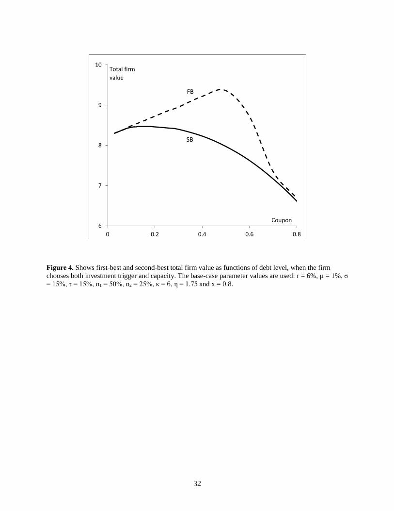
Figure 4 shows the total firm value (first-best and second-best) as a function of the debt level. For

first-best investment policy, the debt level that maximizes total firm value is c = 0.51, resulting in a

leverage ratio of 86.76% and total firm value of 9.3849; for second-best policy, the output is c = 0.159,

leverage ratio = 28.82% and total firm value = 8.4693.

Thus, if we compare the total firm value when both the first-best and second-best investment

policies are at the respective optimal capital structure, we get an agency cost of [9.3849/8.4693 – 1] =

10.81%. This is a significant magnitude, certainly much larger than suggested by previous papers (Mauer

and Ott, 2000, Moyen, 2007, Pawlina, 2010). Thus, if a firm with the greater investment flexibility is not

far from its optimal capital structure when it makes the investment decision, the agency cost of debt

overhang will likely be economically significant.11

Another point worth noting is that the second-best optimal leverage ratio (28.82%) is quite small

compared to typical models of the trade-off theory of capital structure such as Leland (1994), and much

closer to observed leverage ratios in the real world.12 The reason for the firm choosing this low leverage

ratio is that it mitigates future conflicts between equity-holders and debt-holders. This result can

potentially explain the well-known puzzle that structural models lead to optimal leverage ratios that are

much higher than leverage ratios observed in the real world (Leland, 1994).

5. Conclusion

Since first introduced by Myers (1977), the concept of debt overhang or underinvestment has interested

researchers in corporate finance. Although there is widespread agreement about the existence of the debt

overhang agency problem, its practical significance was uncertain because most studies concluded that

the magnitude of the agency cost was insignificant.

11 We call this “greater investment flexibility” because the firm can choose both timing and capacity when making

the investment decision. There are other types of flexibility that have been examined in the literature, which could

also potentially have an impact on the debt overhang problem, e.g., operating flexibility or the ability to temporarily

shut down operations and restart them subsequently (Dixit, 1989, Mauer and Triantis, 1994), and financial flexibility

(Mauer and Triantis, 1994, Titman and Tsyplakov, 2007). 12 According to Berens and Cuny (1995), the typical firm has a leverage ratio in the 25-30% range.

25

This paper takes another look at the debt overhang problem and quantifies the agency cost, using

a contingent-claim model similar to the existing models. We first show that, consistent with the earlier

literature, underinvestment exists when the firm has limited investment flexibility (either investment

timing or size is exogenously specified), but the agency cost is very small, perhaps small enough to be

ignored for practical purposes.

However, with additional investment flexibility (when the firm is allowed to choose both the

timing and size of investment), the agency cost of debt overhang is much higher than previously

estimated figures. Since agency cost is a function of the debt level, we looked at the optimally-levered

firm, and found that the agency cost was economically very significant (about 11% of total firm value in

the base case). Thus it is clear that, in a general setting, the agency cost of debt overhang can be very

large. The main contribution of our paper is to demonstrate that debt overhang generally has a significant

effect on firm value, thus it should not be ignored in the corporate decision-making process.

26

References

Andrade, G. and S.N. Kaplan (1998) How Costly is Financial (Not Economic) Distress? Evidence from

Highly Leveraged Transactions that Became Distressed, Journal of Finance 53, 1443-1493.

Bar-Ilan, A. and W.C. Strange (1996) Investment Lags, American Economic Review 86, 610-622.

Berens, J.L. and C.J. Cuny (1995) The Capital Structure Puzzle Revisited, Review of Financial Studies 8,

1185-1208.

Bertola, G. and R. Caballero (1994) Irreversibility and Aggregate Investment, Review of Economic

Studies 61, 223-246.

Brander, J.A. and T.R Lewis (1986). Oligopoly and Financial Structure: The Limited Liability Effect,

American Economic Review 76, 956-970.

Brealey,R.A. and S.C. Myers (2000) Principles of Corporate Finance. McGraw-Hill, New York, NY.

Chen, H. and G. Manso (2014) Macroeconomic Risk and Debt Overhang, Working Paper.

Childs, P.D., D.C. Mauer and S.F. Ott (2005) Interactions of Corporate Financing and Investment

Decisions: The Effects of Agency Conflicts, Journal of Financial Economics 76, 667-690.

Dangl, T. (1999) Investment and Capacity Choice under Uncertain Demand, European Journal of

Operational Research 117, 415-428.

Davydenko, S.A., I.A. Strebulaev and X. Zhao (2012) A Market-Based Study of the Cost of Default,

Review of Financial Studies 25, 2959-2999.

Dixit, A. (1989) Entry and Exit Decisions under Uncertainty, Journal of Political Economy 97, 620-638.

Dixit, A. and R.S. Pindyck (1994) Investment Under Uncertainty, Princeton University Press, Princeton,

NJ.

Hackbarth, D. and D.C. Mauer (2012) Optimal Priority Structure, Capital Structure, and Investment, Review

of Financial Studies 25, 747-796.

Hennessy, C.A. (2004) Tobin’s Q, Debt Overhang, and Investment, Journal of Finance 59, 1717-1742.

Hirth, S. and M. Uhrig-Homburg (2010) Investment Timing, Liquidity, and Agency Costs of Debt, Journal

of Corporate Finance 16, 243-258.

Jou, J-B. (2001) Corporate Borrowing and Growth Option Value: The Limited Liability Effect, Journal of

Economics and Finance 25, 79-98.

Jou, J-B. and T. Lee (2004) Debt Overhang, Costly Expandability and Reversibility, and Optimal Financial

Structure, Journal of Business Finance and Accounting 31, 1191-1222.

Leland, H. (1994) Risky Debt, Bond Covenants and Optimal Capital Structure, Journal of Finance 49,

1213-1252.

27

Leland, H. (1998) Agency Costs, Risk Management, and Capital Structure, Journal of Finance 53, 1213-

1243.

Lukas, E. and S. Thiergart (2016) Investment under Uncertainty: Does Investment Stimulus Lead to

Underinvestment? Working Paper.

MacKay, P. (2003) Real Flexibility and Financial Structure: An Empirical Analysis, Review of Financial

Studies 16, 1131-1165.

Manso, G. (2008) Investment Reversibility and Agency Cost of Debt, Econometrica 76, 437-42.

Mao, C.X. (2003) Interaction of Debt Agency Problems and Optimal Capital Structure: Theory and

Evidence, Journal of Financial and Quantitative Analysis 38, 399-423.

Mauer, D.C. and S. Ott (2000) Agency Costs, Under-investment, and Optimal Capital Structure: The

Effect of Growth Options to Expand, in: Brennan, M. and Trigeorgis, L. (Eds.), Project Flexibility,

Agency, and Competition, Oxford University Press, New York, 151-180.

Mauer, D.C. and S. Sarkar (2005) Real Options, Agency Conflicts, and Optimal Capital Structure, Journal

of Banking and Finance 29, 1405-1428.

Mauer, D.C. and A. Triantis (1994) Interactions of Corporate Financing and Investment Decisions: A

Dynamic Framework, Journal of Finance 49, 1253-1277.

McDonald, R. and D. Siegel (1986) The Value of Waiting to Invest, Quarterly Journal of Economics 101,

707-727.

Mello, A.S. and J.E. Parsons (1992) Measuring the Agency Cost of Debt, Journal of Finance 47, 1887-

1904.

Moyen, N. (2007) How Big is the Debt Overhang Problem? Journal of Economic Dynamics and Control

31, 433-472.

Myers, S.C. (1977) Determinants of Corporate Borrowing, Journal of Financial Economics 5, 147-175.

Parrino, R. and M.S. Weisbach (1999) Measuring Investment Distortions Arising from Stockholder-

Bondholder Conflicts, Journal of Financial Economics 53, 3-42.

Pawlina, G. (2010) Underinvestment, Capital Structure and Strategic Debt Restructuring, Journal of

Corporate Finance 16, 679-702.

Sarkar, S. and C. Zhang (2015) Underinvestment and the Design of Performance-Sensitive Debt,

International Review of Economics and Finance 37, 240-253.

Titman, S. and S. Tsyplakov (2007) A Dynamic Model of Optimal Capital Structure, Review of Finance

11, 401-451.

28

Table 1. Underinvestment in the three scenarios

Base-case parameter values: r = 6%, µ = 1%, σ = 15%, τ = 15%, α1 = 50%, α2 = 25%, κ = 6, η =

1.75, c = 0.3 and x = 0.8.

Underinvestment as measured by

%ΔPV(Inv) Agency cost

1. Q exogenous, x* endogenous 3.27% 0.03%

2. x* exogenous, Q endogenous 0.46% 0.001%

3. Both Q and x* endogenous 2.05% 6.69%

Table 2. Effect of investment cost parameters η and κ

Base-case parameter values: r = 6%, µ = 1%, σ = 15%, τ = 15%, α1 = 50%, α2 = 25%, κ = 6, η =

1.75, c = 0.3 and x = 0.8 (Q = 3 for “Not flexible” and the optimal capacity for “Flexible”).

%ΔPV(Inv) Agency cost

η Not flexible Flexible η Not flexible Flexible

1.75 3.27% 2.05% 1.75 0.03% 6.69%

1.9 2.22% 6.76% 1.9 0.014% 4.25%

%ΔPV(Inv) Agency cost

κ Not flexible Flexible κ Not flexible Flexible

6 3.27% 2.05% 6 0.03% 6.69%

8 1.62% 22.05% 8 0.01% 13.64%

29

Figures 1(a), 1(b) and 1(c). Shows results with varying debt levels, when capacity is fixed and the firm

chooses investment trigger. Part (a) shows both first-best and second-best triggers, part (b) shows first-

best and second-best levels of expected investment (in present value terms), and part (c) shows two

measures of the degree of underinvestment, difference in present value of investment and agency cost.

The base-case parameter values are used: r = 6%, µ = 1%, σ = 15%, τ = 15%, α1 = 50%, α2 = 25%, κ = 6,

η = 1.75, x = 0.8 and Q =3.

1.3

1.35

1.4

1.45

1.5

0 0.2 0.4 0.6 0.8 1

Coupon

x*

SB

FB

2

4

6

8

10

12

0 0.2 0.4 0.6 0.8 1

Coupon

PV(Inv)

SBFB

0

2

4

6

8

10

0 0.5 1Coupon

%ΔPV(Inv)

Agency cost (%)

30

Figures 2(a), 2(b) and 2(c). Shows results with varying debt levels, when investment trigger is fixed and

firm chooses investment size or capacity. Part (a) shows both first-best and second-best capacity, part (b)

shows first-best and second-best levels of expected investment (in present value terms), and part (c)

shows two measures of the degree of underinvestment, difference in present value of investment and

agency cost. The base-case parameter values are used: r = 6%, µ = 1%, σ = 15%, τ = 15%, α1 = 50%, α2 =

25%, κ = 6, η = 1.75 and x* = x = 0.9.

1.6

1.65

1.7

0 0.4 0.8Coupon

Q*

FB

SB

13.6

14

14.4

14.8

15.2

0 0.4 0.8Coupon

PV(Inv)

FB

SB

-1

1

3

5

7

0 0.4 0.8Coupon

%ΔPV(Inv)

Agency cost (%)

31

Figures 3(a), 3(b) and 3(c). Shows results with varying debt levels, when the firm chooses both

investment trigger and capacity. Part (a) shows both first-best and second-best investment trigger, part (b)

shows first-best and second-best capacity, and part (c) shows two measures of the degree of

underinvestment, difference in present value of investment and agency cost. The base-case parameter

values are used: r = 6%, µ = 1%, σ = 15%, τ = 15%, α1 = 50%, α2 = 25%, κ = 6, η = 1.75 and x = 0.8.

0.5

1

1.5

2

2.5

0.2 0.4 0.6 0.8 1

Coupon

Investmenttrigger

SB

FB

0

1

2

3

4

5

6

0.2 0.4 0.6 0.8 1

Coupon

Capacity

SB

FB

0

5

10

15

20

25

30

0.2 0.6 1Coupon

Agencycost (%)

%ΔPV(Inv)

32

Figure 4. Shows first-best and second-best total firm value as functions of debt level, when the firm

chooses both investment trigger and capacity. The base-case parameter values are used: r = 6%, µ = 1%, σ

= 15%, τ = 15%, α1 = 50%, α2 = 25%, κ = 6, η = 1.75 and x = 0.8.

6

7

8

9

10

0 0.2 0.4 0.6 0.8

FB

SB

Total firm

value

Coupon