Dealing with VarianceAn Efficient Minibatch Acceptance Test for Metropolis-Hastings

Daniel SeitaUniversity of California, Berkeley

Uncertainty in Artificial IntelligenceAugust 14, 2017

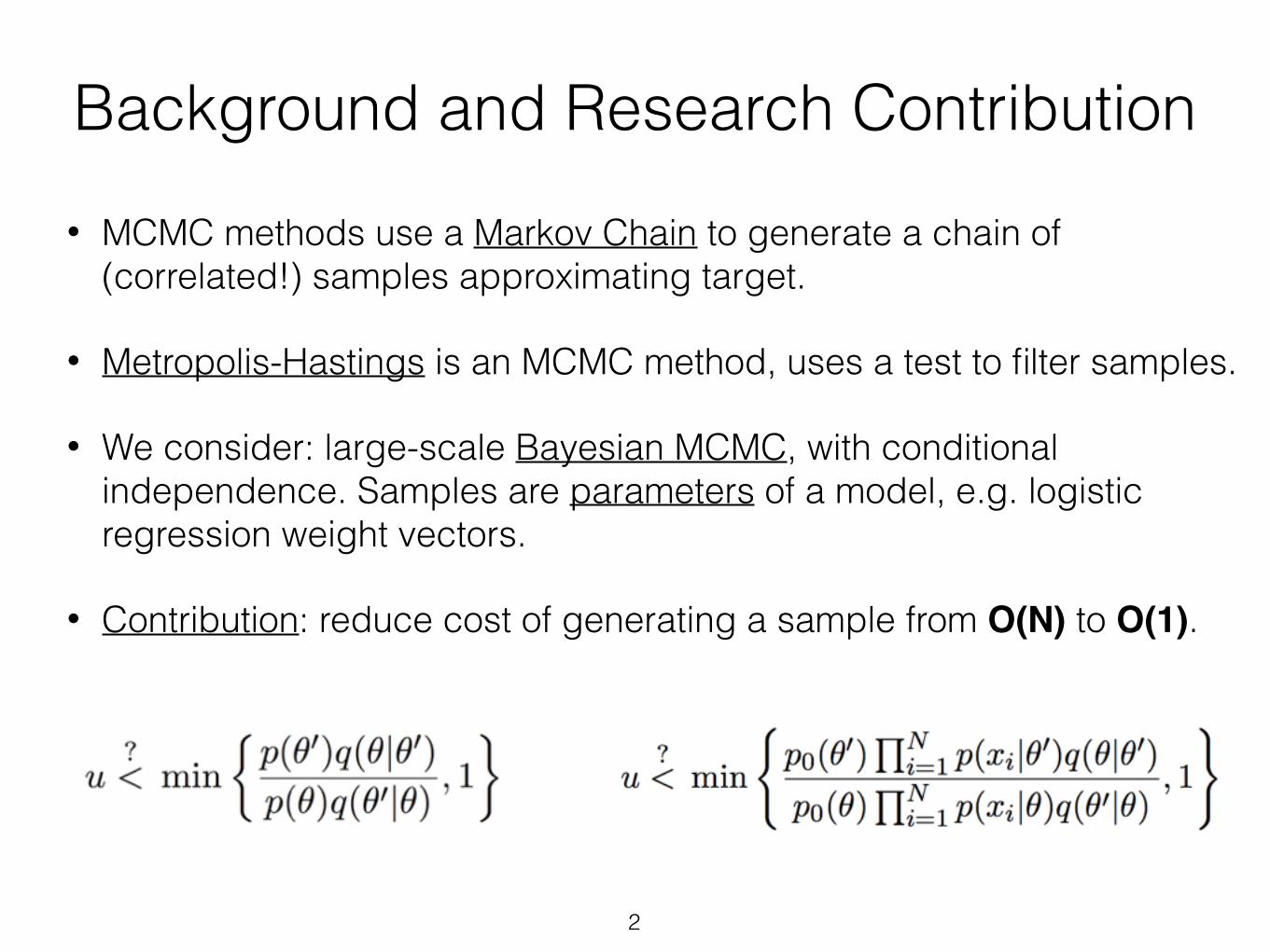
• MCMC methods use a Markov Chain to generate a chain of (correlated!) samples approximating target.

• Metropolis-Hastings is an MCMC method, uses a test to filter samples.

• We consider: large-scale Bayesian MCMC, with conditional independence. Samples are parameters of a model, e.g. logistic regression weight vectors.

• Contribution: reduce cost of generating a sample from O(N) to O(1).

Background and Research Contribution

2

Data Deluge: SGD and MCMC

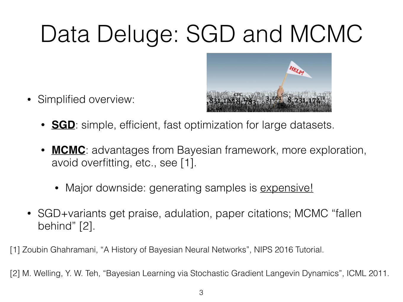
• Simplified overview:

• SGD: simple, efficient, fast optimization for large datasets.

• MCMC: advantages from Bayesian framework, more exploration, avoid overfitting, etc., see [1].

• Major downside: generating samples is expensive!

• SGD+variants get praise, adulation, paper citations; MCMC “fallen behind” [2].

3

[1] Zoubin Ghahramani, “A History of Bayesian Neural Networks”, NIPS 2016 Tutorial.

[2] M. Welling, Y. W. Teh, “Bayesian Learning via Stochastic Gradient Langevin Dynamics”, ICML 2011.

What This Paper Doesn't Do• Generate independent samples from a model posterior in O(1).

• Independent model samples require data samples in general [1].

• Note: Gibbs samplers (for LDA, CRP etc) generate posterior samples in O(1) input samples [2]??

• Minibatch samples can be generated in O(1) when either

• Step size is reduced (correlated samples)

• Temperature is increased

• Hamiltonian Dynamics is used - M-H test need only correct errors

4

[1] S. Mandt, M.D. Hoffman, D. Blei, “Stochastic Gradient Descent as Approximate Bayesian Inference,” arXiv 2017.

[2] C. Dupuy, F. Bach, “Online but Accurate Inference for Latent Variable Models with Local Gibbs Sampling,” arXiv 2016.

Ω(N )

What This Paper Doesn't Do• Generate independent samples from a model posterior in O(1).

• Independent model samples require data samples in general [1].

• Note: Gibbs samplers (for LDA, CRP etc) generate posterior samples in O(1) input samples [2] - step size is O(1/N)

• Minibatch samples can be generated in O(1) when either

• Step size is reduced (correlated samples)

• Temperature is increased

• Hamiltonian Dynamics is used - M-H test need only correct errors

5

[1] S. Mandt, M.D. Hoffman, D. Blei, “Stochastic Gradient Descent as Approximate Bayesian Inference,” arXiv 2017.

[2] C. Dupuy, F. Bach, “Online but Accurate Inference for Latent Variable Models with Local Gibbs Sampling,” arXiv 2016.

Ω(N )

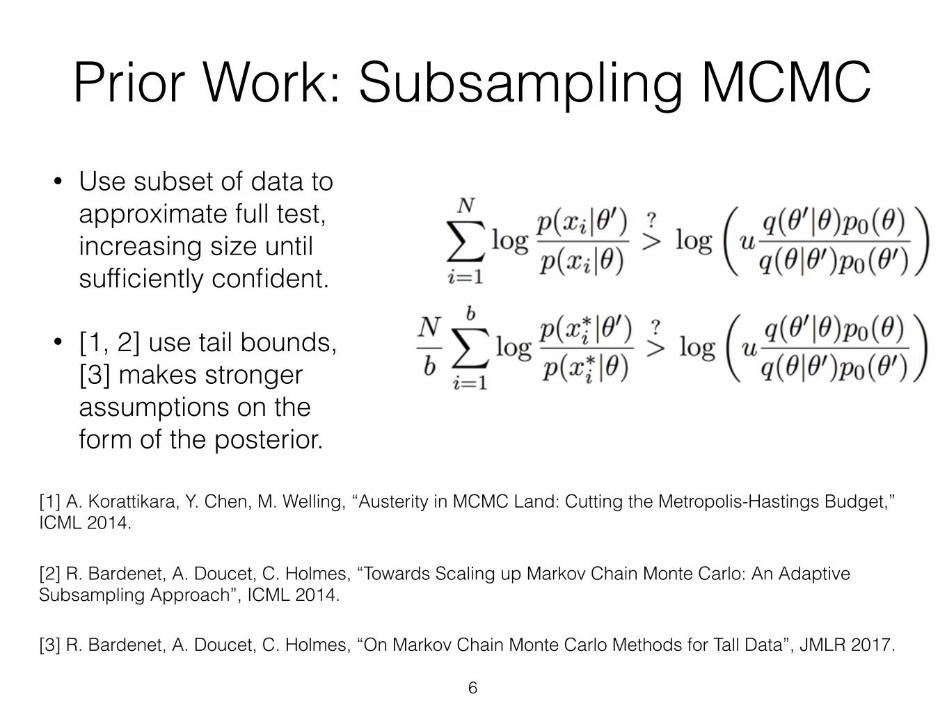
Prior Work: Subsampling MCMC

6

[1] A. Korattikara, Y. Chen, M. Welling, “Austerity in MCMC Land: Cutting the Metropolis-Hastings Budget,” ICML 2014.

[2] R. Bardenet, A. Doucet, C. Holmes, “Towards Scaling up Markov Chain Monte Carlo: An Adaptive Subsampling Approach”, ICML 2014.

[3] R. Bardenet, A. Doucet, C. Holmes, “On Markov Chain Monte Carlo Methods for Tall Data”, JMLR 2017.

• Use subset of data to approximate full test, increasing size until sufficiently confident.

• [1, 2] use tail bounds, [3] makes stronger assumptions on the form of the posterior.

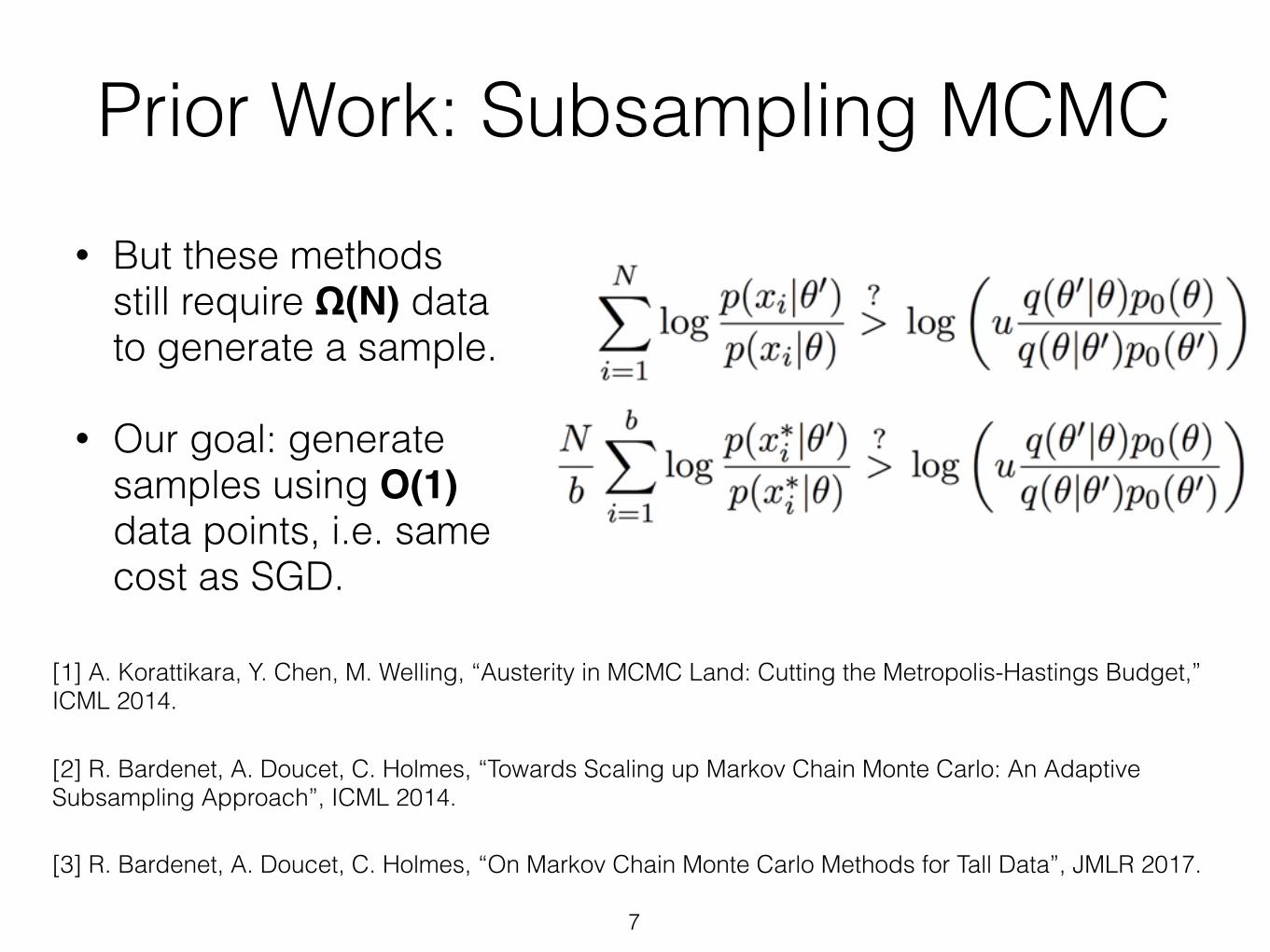
• But these methods still require Ω(N) data to generate a sample.

• Our goal: generate samples using O(1) data points, i.e. same cost as SGD.

7

[1] A. Korattikara, Y. Chen, M. Welling, “Austerity in MCMC Land: Cutting the Metropolis-Hastings Budget,” ICML 2014.

[2] R. Bardenet, A. Doucet, C. Holmes, “Towards Scaling up Markov Chain Monte Carlo: An Adaptive Subsampling Approach”, ICML 2014.

[3] R. Bardenet, A. Doucet, C. Holmes, “On Markov Chain Monte Carlo Methods for Tall Data”, JMLR 2017.

Prior Work: Subsampling MCMC

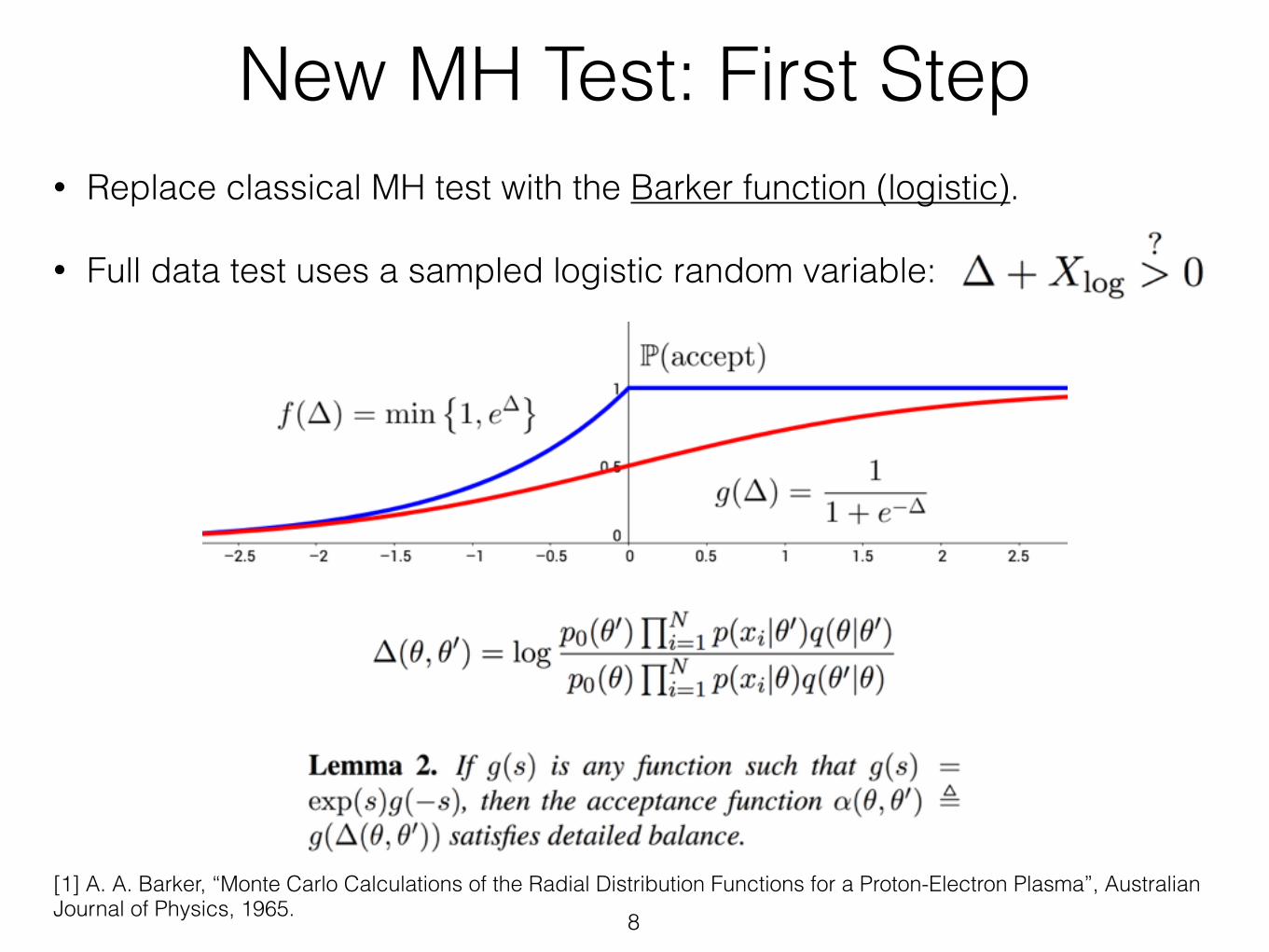
New MH Test: First Step

8[1] A. A. Barker, “Monte Carlo Calculations of the Radial Distribution Functions for a Proton-Electron Plasma”, Australian Journal of Physics, 1965.

• Replace classical MH test with the Barker function (logistic).

• Full data test uses a sampled logistic random variable:

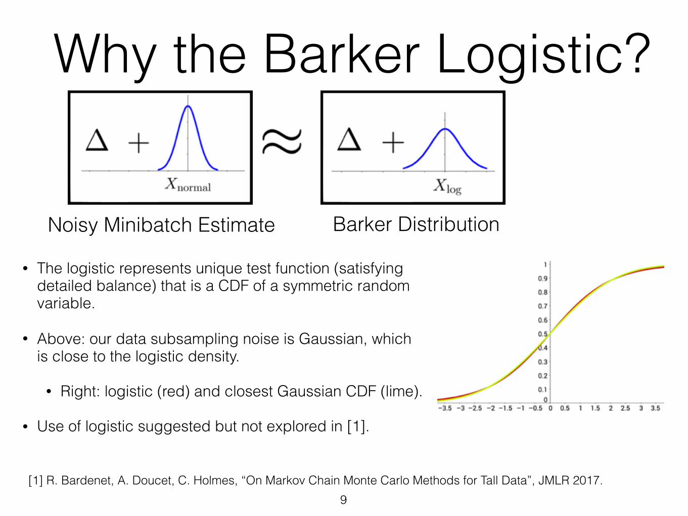
Why the Barker Logistic?

• The logistic represents unique test function (satisfying detailed balance) that is a CDF of a symmetric random variable.

• Above: our data subsampling noise is Gaussian, which is close to the logistic density.

• Right: logistic (red) and closest Gaussian CDF (lime).

• Use of logistic suggested but not explored in [1].

9[1] R. Bardenet, A. Doucet, C. Holmes, “On Markov Chain Monte Carlo Methods for Tall Data”, JMLR 2017.

Noisy Minibatch Estimate Barker Distribution

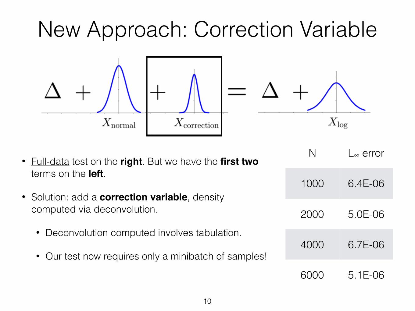
• Full-data test on the right. But we have the first two terms on the left.

• Solution: add a correction variable, density computed via deconvolution.

• Deconvolution computed involves tabulation.

• Our test now requires only a minibatch of samples!

New Approach: Correction Variable

10

N L∞ error

1000 6.4E-06

2000 5.0E-06

4000 6.7E-06

6000 5.1E-06

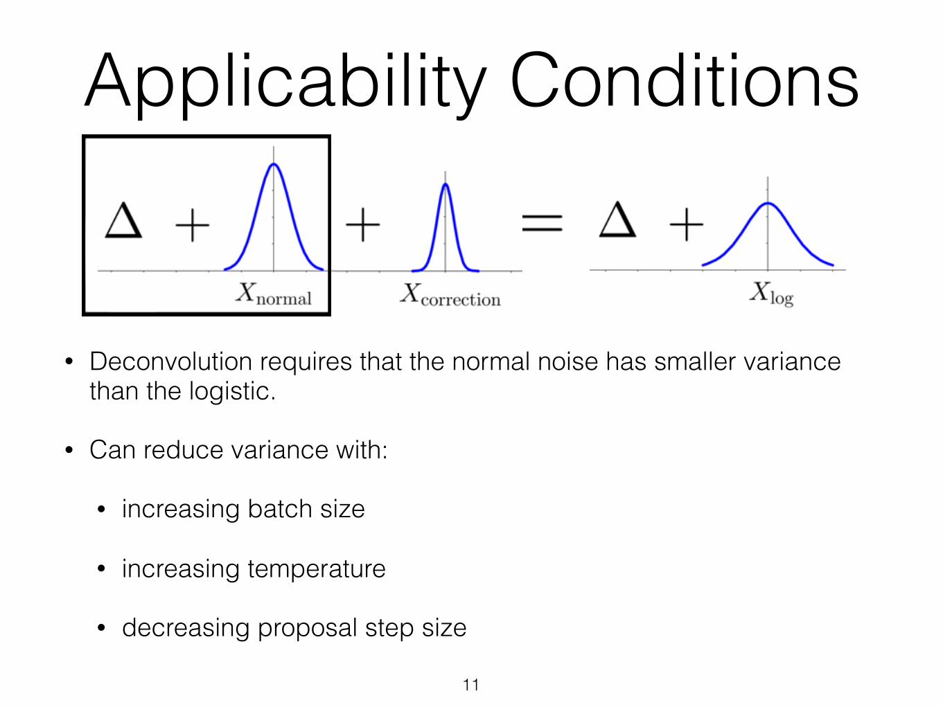
• Deconvolution requires that the normal noise has smaller variance than the logistic.

• Can reduce variance with:

• increasing batch size

• increasing temperature

• decreasing proposal step size

Applicability Conditions

11

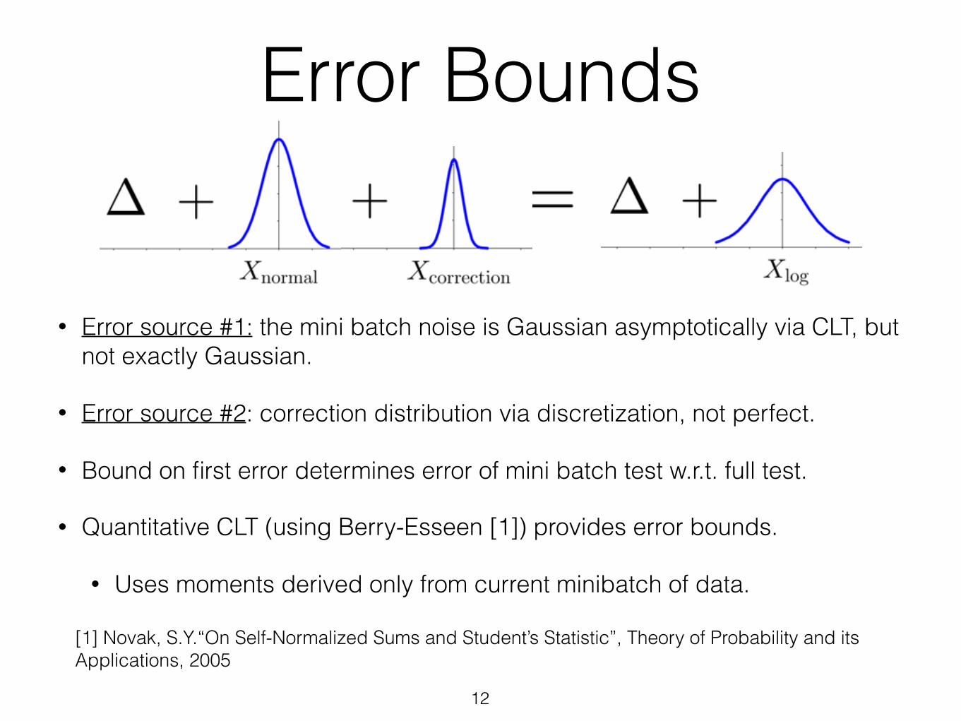
• Error source #1: the mini batch noise is Gaussian asymptotically via CLT, but not exactly Gaussian.

• Error source #2: correction distribution via discretization, not perfect.

• Bound on first error determines error of mini batch test w.r.t. full test.

• Quantitative CLT (using Berry-Esseen [1]) provides error bounds.

• Uses moments derived only from current minibatch of data.

[1] Novak, S.Y.“On Self-Normalized Sums and Student’s Statistic”, Theory of Probability and its Applications, 2005

Error Bounds

12

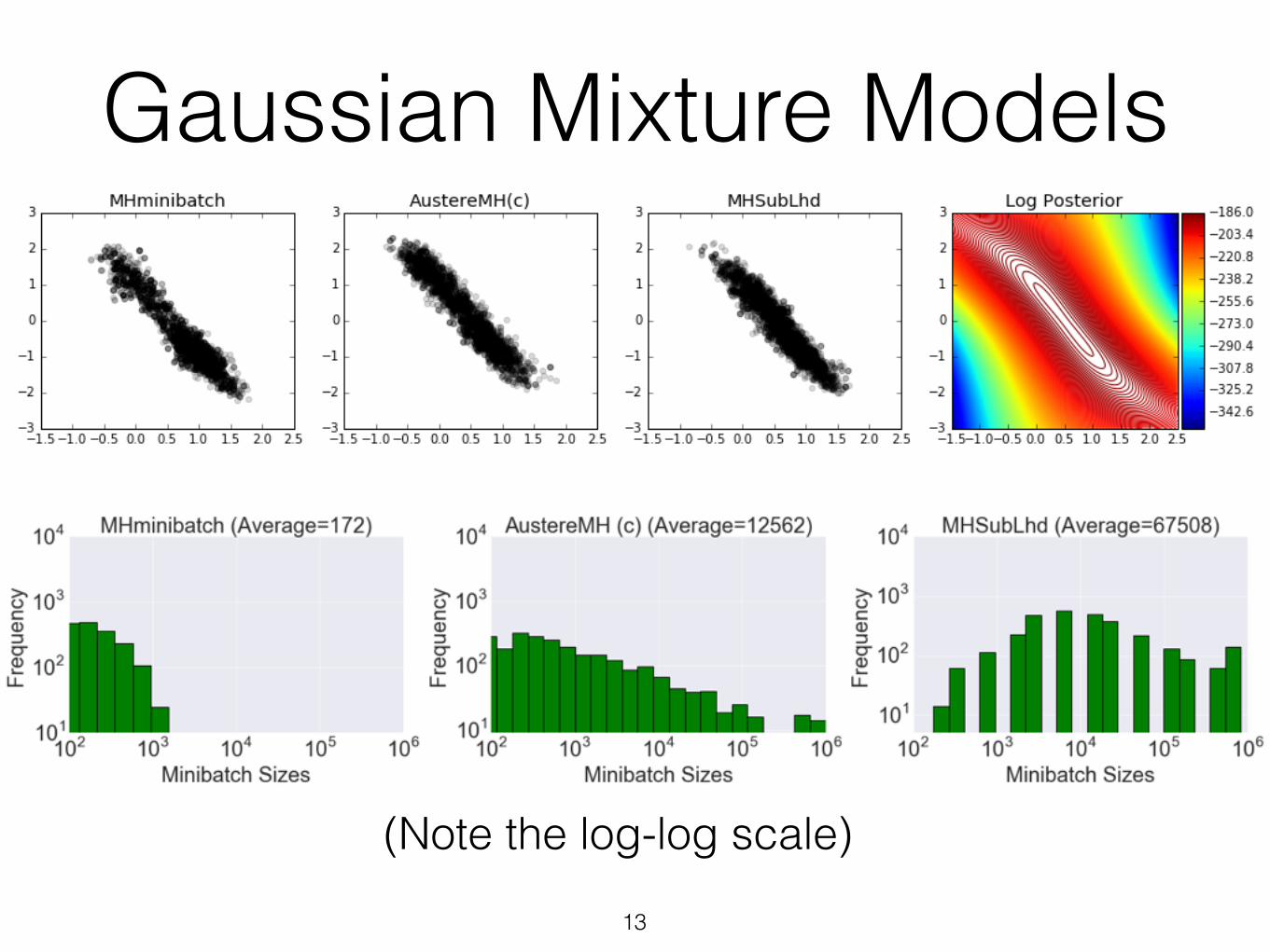
Gaussian Mixture Models

13

(Note the log-log scale)

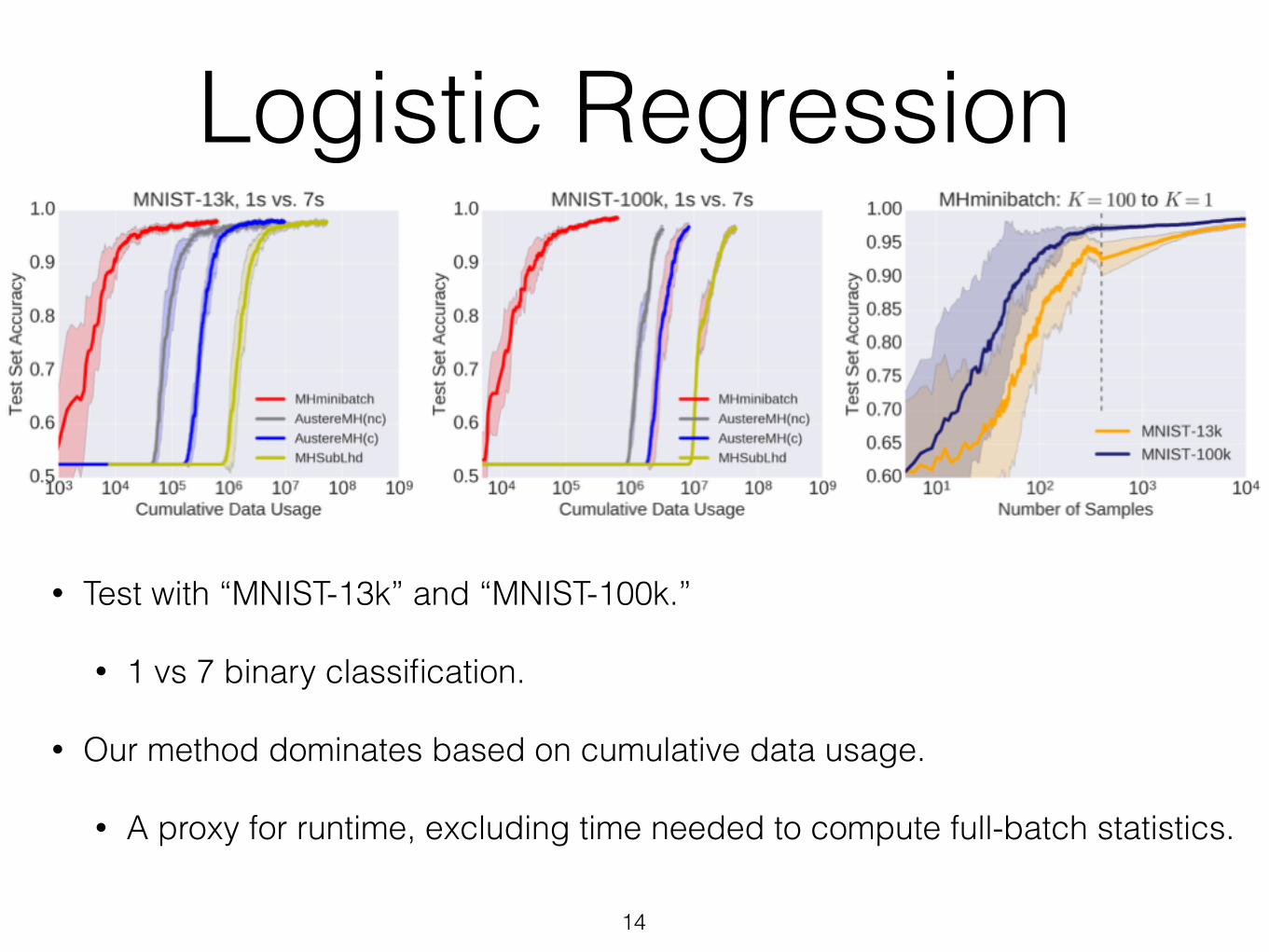
Logistic Regression

• Test with “MNIST-13k” and “MNIST-100k.”

• 1 vs 7 binary classification.

• Our method dominates based on cumulative data usage.

• A proxy for runtime, excluding time needed to compute full-batch statistics.

14

Conclusions• Derived and analyzed a minibatch MH test.

• Uses Barker test plus novel correction variable.

• Excellent performance on Gaussian Mixture Model and Logistic Regression experiments.

• Consumes substantially less data than prior methods, uses minibatches (constant expected subset size).

• Implemented in BIDMach. [1]

15

[1] https://github.com/BIDData/BIDMach

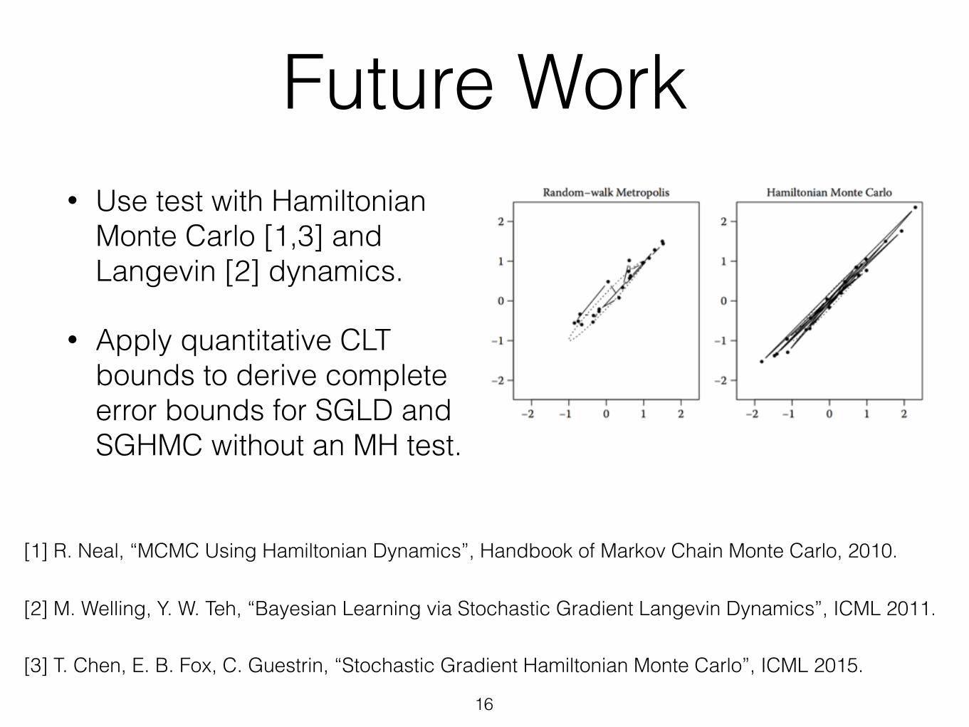
Future Work• Use test with Hamiltonian

Monte Carlo [1,3] and Langevin [2] dynamics.

• Apply quantitative CLT bounds to derive complete error bounds for SGLD and SGHMC without an MH test.

16

[1] R. Neal, “MCMC Using Hamiltonian Dynamics”, Handbook of Markov Chain Monte Carlo, 2010.

[2] M. Welling, Y. W. Teh, “Bayesian Learning via Stochastic Gradient Langevin Dynamics”, ICML 2011.

[3] T. Chen, E. B. Fox, C. Guestrin, “Stochastic Gradient Hamiltonian Monte Carlo”, ICML 2015.

Thank You!• Thanks to a hard-working team, lots of ideas refined,

tuned, and improved.

• Also, thank you for your attention.

17

Daniel Seita Xinlei Pan Haoyu Chen John Canny

Don’t forget to check out our blog post! Search “Berkeley AI Research Blog”. http://bair.berkeley.edu/blog/2017/08/02/minibatch-metropolis-hastings/

These slides are also available on my academic website. https://people.eecs.berkeley.edu/~seita/