VarianceFrom Wikipedia, the free encyclopedia

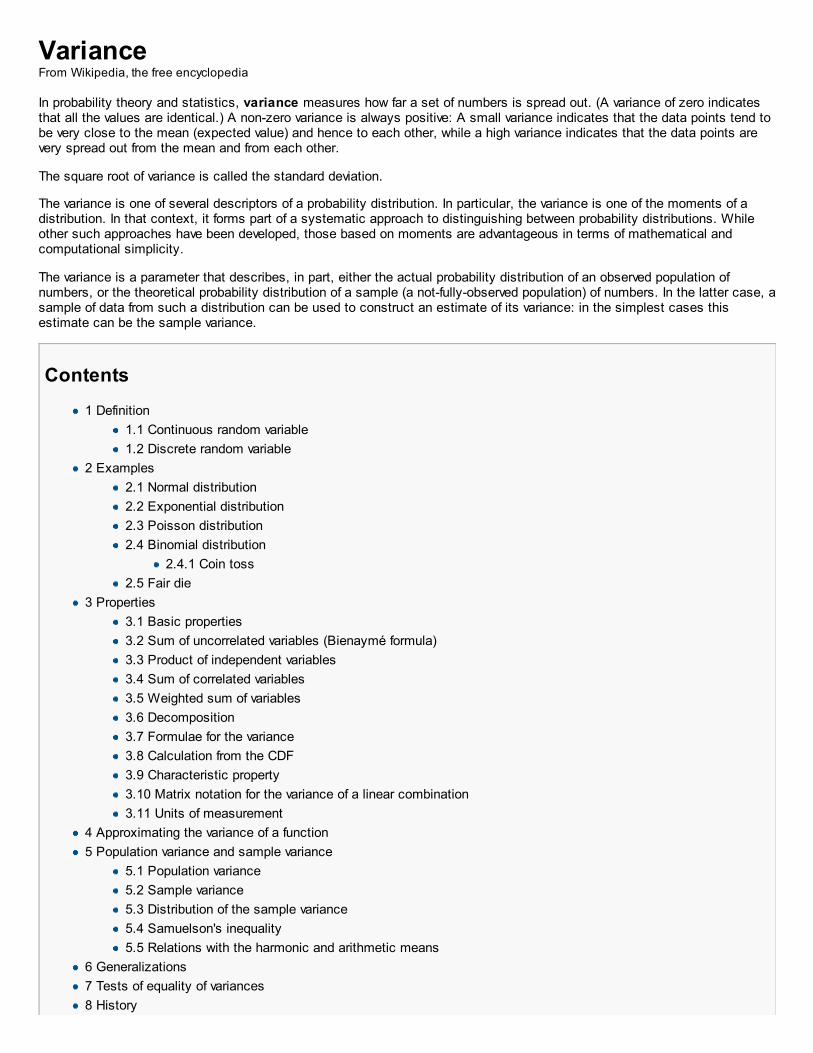
In probability theory and statistics, variance measures how far a set of numbers is spread out. (A variance of zero indicatesthat all the values are identical.) A non-zero variance is always positive: A small variance indicates that the data points tend tobe very close to the mean (expected value) and hence to each other, while a high variance indicates that the data points arevery spread out from the mean and from each other.

The square root of variance is called the standard deviation.

The variance is one of several descriptors of a probability distribution. In particular, the variance is one of the moments of adistribution. In that context, it forms part of a systematic approach to distinguishing between probability distributions. Whileother such approaches have been developed, those based on moments are advantageous in terms of mathematical andcomputational simplicity.

The variance is a parameter that describes, in part, either the actual probability distribution of an observed population ofnumbers, or the theoretical probability distribution of a sample (a not-fully-observed population) of numbers. In the latter case, asample of data from such a distribution can be used to construct an estimate of its variance: in the simplest cases thisestimate can be the sample variance.

Contents

1 Definition

1.1 Continuous random variable

1.2 Discrete random variable

2 Examples

2.1 Normal distribution

2.2 Exponential distribution

2.3 Poisson distribution

2.4 Binomial distribution

2.4.1 Coin toss

2.5 Fair die

3 Properties

3.1 Basic properties

3.2 Sum of uncorrelated variables (Bienaymé formula)

3.3 Product of independent variables

3.4 Sum of correlated variables

3.5 Weighted sum of variables

3.6 Decomposition

3.7 Formulae for the variance

3.8 Calculation from the CDF

3.9 Characteristic property

3.10 Matrix notation for the variance of a linear combination

3.11 Units of measurement

4 Approximating the variance of a function

5 Population variance and sample variance

5.1 Population variance

5.2 Sample variance

5.3 Distribution of the sample variance

5.4 Samuelson's inequality

5.5 Relations with the harmonic and arithmetic means

6 Generalizations

7 Tests of equality of variances

8 History

9 Moment of inertia

10 See also

11 Notes

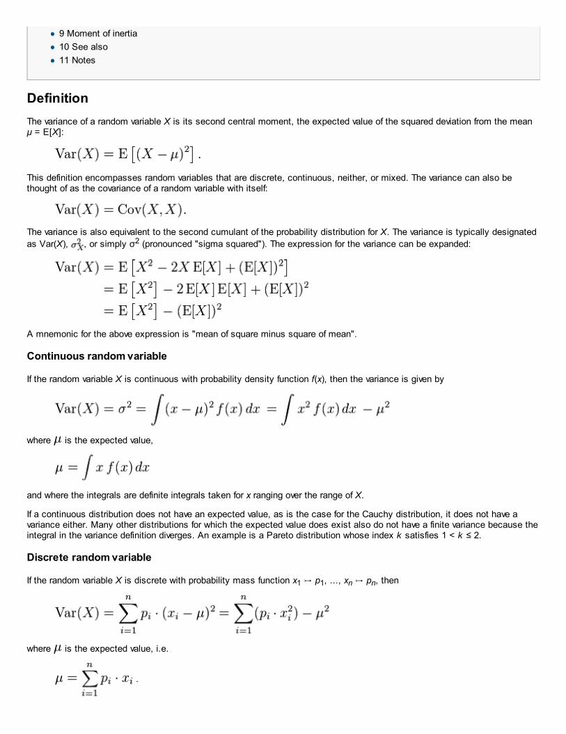
Definition

The variance of a random variable X is its second central moment, the expected value of the squared deviation from the meanμ = E[X]:

This definition encompasses random variables that are discrete, continuous, neither, or mixed. The variance can also bethought of as the covariance of a random variable with itself:

The variance is also equivalent to the second cumulant of the probability distribution for X. The variance is typically designated

as Var(X), , or simply σ2 (pronounced "sigma squared"). The expression for the variance can be expanded:

A mnemonic for the above expression is "mean of square minus square of mean".

Continuous random variable

If the random variable X is continuous with probability density function f(x), then the variance is given by

where is the expected value,

and where the integrals are definite integrals taken for x ranging over the range of X.

If a continuous distribution does not have an expected value, as is the case for the Cauchy distribution, it does not have avariance either. Many other distributions for which the expected value does exist also do not have a finite variance because theintegral in the variance definition diverges. An example is a Pareto distribution whose index k satisfies 1 < k ≤ 2.

Discrete random variable

If the random variable X is discrete with probability mass function x1 ↦ p1, ..., xn ↦ pn, then

where is the expected value, i.e.

.

(When such a discrete weighted variance is specified by weights whose sum is not 1, then one divides by the sum of theweights.)

The variance of a set of n equally likely values can be written as

The variance of a set of n equally likely values can be equivalently expressed, without directly referring to the mean, in terms of

squared deviations of all points from each other:[1]

Examples

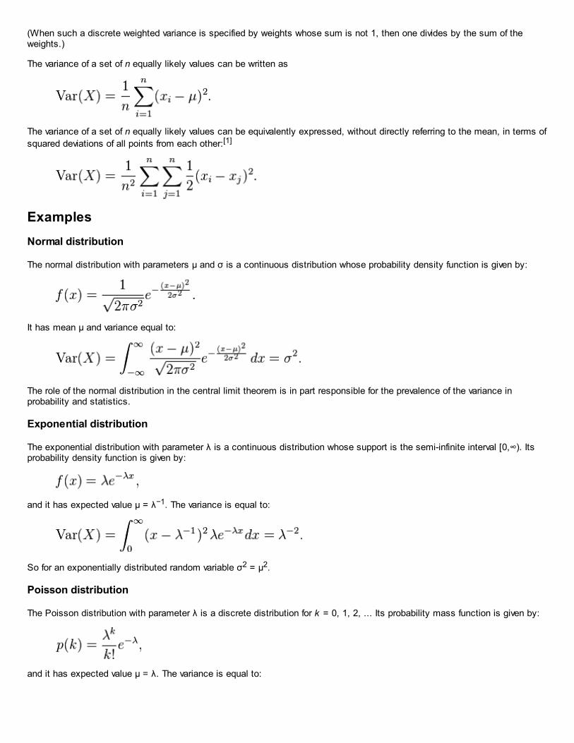
Normal distribution

The normal distribution with parameters μ and σ is a continuous distribution whose probability density function is given by:

It has mean μ and variance equal to:

The role of the normal distribution in the central limit theorem is in part responsible for the prevalence of the variance inprobability and statistics.

Exponential distribution

The exponential distribution with parameter λ is a continuous distribution whose support is the semi-infinite interval [0,∞). Itsprobability density function is given by:

and it has expected value μ = λ−1. The variance is equal to:

So for an exponentially distributed random variable σ2 = μ2.

Poisson distribution

The Poisson distribution with parameter λ is a discrete distribution for k = 0, 1, 2, ... Its probability mass function is given by:

and it has expected value μ = λ. The variance is equal to:

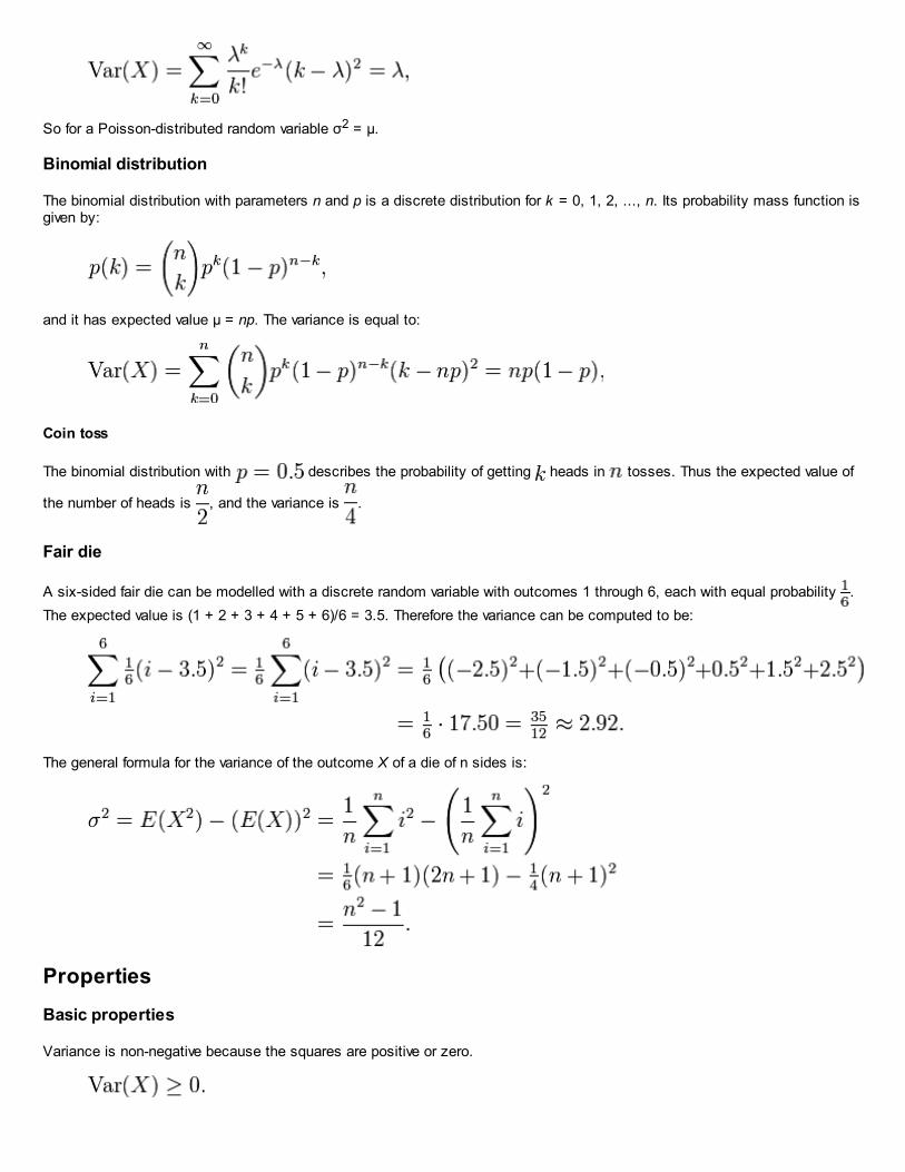
So for a Poisson-distributed random variable σ2 = μ.

Binomial distribution

The binomial distribution with parameters n and p is a discrete distribution for k = 0, 1, 2, ..., n. Its probability mass function isgiven by:

and it has expected value μ = np. The variance is equal to:

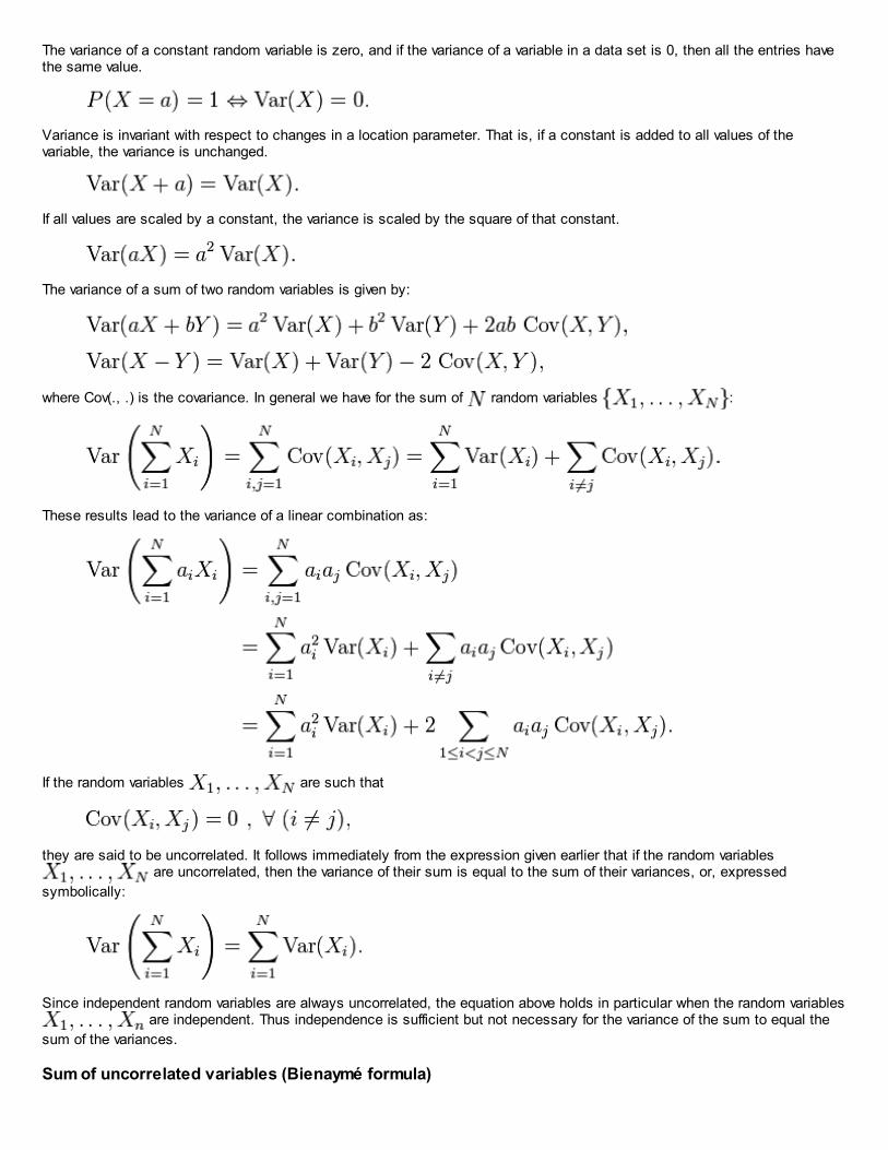
Coin toss

The binomial distribution with describes the probability of getting heads in tosses. Thus the expected value of

the number of heads is , and the variance is .

Fair die

A six-sided fair die can be modelled with a discrete random variable with outcomes 1 through 6, each with equal probability .

The expected value is (1 + 2 + 3 + 4 + 5 + 6)/6 = 3.5. Therefore the variance can be computed to be:

The general formula for the variance of the outcome X of a die of n sides is:

Properties

Basic properties

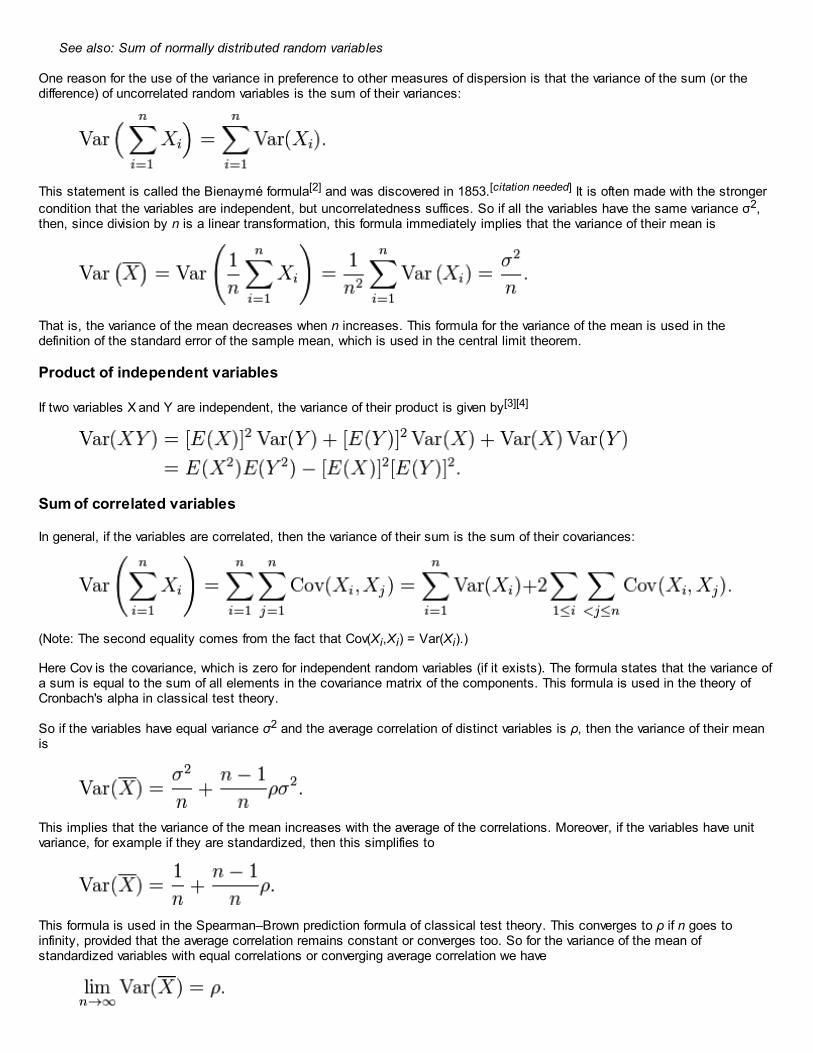
Variance is non-negative because the squares are positive or zero.

The variance of a constant random variable is zero, and if the variance of a variable in a data set is 0, then all the entries have

The variance of a constant random variable is zero, and if the variance of a variable in a data set is 0, then all the entries havethe same value.

Variance is invariant with respect to changes in a location parameter. That is, if a constant is added to all values of thevariable, the variance is unchanged.

If all values are scaled by a constant, the variance is scaled by the square of that constant.

The variance of a sum of two random variables is given by:

where Cov(., .) is the covariance. In general we have for the sum of random variables :

These results lead to the variance of a linear combination as:

If the random variables are such that

they are said to be uncorrelated. It follows immediately from the expression given earlier that if the random variables are uncorrelated, then the variance of their sum is equal to the sum of their variances, or, expressed

symbolically:

Since independent random variables are always uncorrelated, the equation above holds in particular when the random variables are independent. Thus independence is sufficient but not necessary for the variance of the sum to equal the

sum of the variances.

Sum of uncorrelated variables (Bienaymé formula)

See also: Sum of normally distributed random variables

One reason for the use of the variance in preference to other measures of dispersion is that the variance of the sum (or thedifference) of uncorrelated random variables is the sum of their variances:

This statement is called the Bienaymé formula[2] and was discovered in 1853.[citation needed] It is often made with the stronger

condition that the variables are independent, but uncorrelatedness suffices. So if all the variables have the same variance σ2,then, since division by n is a linear transformation, this formula immediately implies that the variance of their mean is

That is, the variance of the mean decreases when n increases. This formula for the variance of the mean is used in thedefinition of the standard error of the sample mean, which is used in the central limit theorem.

Product of independent variables

If two variables X and Y are independent, the variance of their product is given by[3][4]

Sum of correlated variables

In general, if the variables are correlated, then the variance of their sum is the sum of their covariances:

(Note: The second equality comes from the fact that Cov(Xi,Xi) = Var(Xi).)

Here Cov is the covariance, which is zero for independent random variables (if it exists). The formula states that the variance ofa sum is equal to the sum of all elements in the covariance matrix of the components. This formula is used in the theory ofCronbach's alpha in classical test theory.

So if the variables have equal variance σ2 and the average correlation of distinct variables is ρ, then the variance of their meanis

This implies that the variance of the mean increases with the average of the correlations. Moreover, if the variables have unitvariance, for example if they are standardized, then this simplifies to

This formula is used in the Spearman–Brown prediction formula of classical test theory. This converges to ρ if n goes toinfinity, provided that the average correlation remains constant or converges too. So for the variance of the mean ofstandardized variables with equal correlations or converging average correlation we have

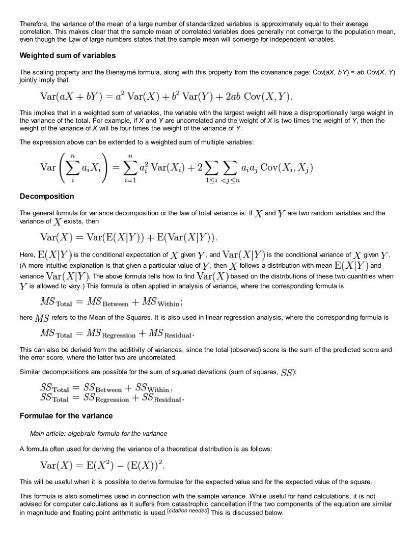
Therefore, the variance of the mean of a large number of standardized variables is approximately equal to their averagecorrelation. This makes clear that the sample mean of correlated variables does generally not converge to the population mean,even though the Law of large numbers states that the sample mean will converge for independent variables.

Weighted sum of variables

The scaling property and the Bienaymé formula, along with this property from the covariance page: Cov(aX, bY) = ab Cov(X, Y)jointly imply that

This implies that in a weighted sum of variables, the variable with the largest weight will have a disproportionally large weight inthe variance of the total. For example, if X and Y are uncorrelated and the weight of X is two times the weight of Y, then theweight of the variance of X will be four times the weight of the variance of Y.

The expression above can be extended to a weighted sum of multiple variables:

Decomposition

The general formula for variance decomposition or the law of total variance is: If and are two random variables and thevariance of exists, then

Here, is the conditional expectation of given , and is the conditional variance of given .

(A more intuitive explanation is that given a particular value of , then follows a distribution with mean and

variance . The above formula tells how to find based on the distributions of these two quantities when

is allowed to vary.) This formula is often applied in analysis of variance, where the corresponding formula is

here refers to the Mean of the Squares. It is also used in linear regression analysis, where the corresponding formula is

This can also be derived from the additivity of variances, since the total (observed) score is the sum of the predicted score andthe error score, where the latter two are uncorrelated.

Similar decompositions are possible for the sum of squared deviations (sum of squares, ):

Formulae for the variance

Main article: algebraic formula for the variance

A formula often used for deriving the variance of a theoretical distribution is as follows:

This will be useful when it is possible to derive formulae for the expected value and for the expected value of the square.

This formula is also sometimes used in connection with the sample variance. While useful for hand calculations, it is notadvised for computer calculations as it suffers from catastrophic cancellation if the two components of the equation are similar

in magnitude and floating point arithmetic is used.[citation needed] This is discussed below.

Calculation from the CDF

The population variance for a non-negative random variable can be expressed in terms of the cumulative distribution function Fusing

where H(u) = 1 − F(u) is the right tail function. This expression can be used to calculate the variance in situations where theCDF, but not the density, can be conveniently expressed.

Characteristic property

The second moment of a random variable attains the minimum value when taken around the first moment (i.e., mean) of the

random variable, i.e. . Conversely, if a continuous function satisfies

for all random variables X, then it is necessarily of the form

, where a > 0. This also holds in the multidimensional case.[5]

Matrix notation for the variance of a linear combination

Let's define as a column vector of n random variables , and c as a column vector of N scalars .

Therefore is a linear combination of these random variables, where denotes the transpose of vector . Let also be

the variance-covariance matrix of the vector X. The variance of is given by:[6]

Units of measurement

Unlike expected absolute deviation, the variance of a variable has units that are the square of the units of the variable itself. Forexample, a variable measured in inches will have a variance measured in square inches. For this reason, describing data setsvia their standard deviation or root mean square deviation is often preferred over using the variance. In the dice example thestandard deviation is √2.9 ≈ 1.7, slightly larger than the expected absolute deviation of 1.5.

The standard deviation and the expected absolute deviation can both be used as an indicator of the "spread" of a distribution.The standard deviation is more amenable to algebraic manipulation than the expected absolute deviation, and, together withvariance and its generalization covariance, is used frequently in theoretical statistics; however the expected absolute deviationtends to be more robust as it is less sensitive to outliers arising from measurement anomalies or an unduly heavy-taileddistribution.

Approximating the variance of a function

The delta method uses second-order Taylor expansions to approximate the variance of a function of one or more randomvariables: see Taylor expansions for the moments of functions of random variables. For example, the approximate variance of afunction of one variable is given by

provided that f is twice differentiable and that the mean and variance of X are finite.

Population variance and sample variance

See also: Unbiased estimation of standard deviation

Real-world distributions such as the distribution of yesterday's rain throughout the day are typically not fully known, unlike thebehavior of perfect dice or an ideal distribution such as the normal distribution, because it is impractical to account for everyraindrop. Instead one estimates the mean and variance of the whole distribution as the computed mean and variance of asample of n observations drawn suitably randomly from the whole sample space, in this example the set of all measurementsof yesterday's rainfall in all available rain gauges.

This method of estimation is close to optimal, with the caveat that it underestimates the variance by a factor of (n − 1) / n. (Forexample, when n = 1 the variance of a single observation is obviously zero regardless of the true variance). This gives a biaswhich should be corrected for when n is small by multiplying by n / (n − 1). If the mean is determined in some other way thanfrom the same samples used to estimate the variance then this bias does not arise and the variance can safely be estimatedas that of the samples.

Population variance

In general, the population variance of a finite population of size N with values xi is given by

where

is the population mean. The population variance therefore is the variance of the underlying probability distribution. In this sense,the concept of population can be extended to continuous random variables with infinite populations.

Sample variance

In many practical situations, the true variance of a population is not known a priori and must be computed somehow. Whendealing with extremely large populations, it is not possible to count every object in the population, so the computation must be

performed on a sample of the population.[7] Sample variance can also be applied to the estimation of the variance of acontinuous distribution from a sample of that distribution.

We take a sample with replacement of n values y1, ..., yn from the population, where n < N, and estimate the variance on the

basis of this sample.[8] Directly taking the variance of the sample gives:

Here, denotes the sample mean:

Since the yi are selected randomly, both and are random variables. Their expected values can be evaluated by summing

over the ensemble of all possible samples {yi} from the population. For this gives:

Hence gives an estimate of the population variance that is biased by a factor of (n-1)/n. For this reason, is referred to as

the biased sample variance. Correcting for this bias yields the unbiased sample variance:

Either estimator may be simply referred to as the sample variance when the version can be determined by context. The sameproof is also applicable for samples taken from a continuous probability distribution.

The use of the term n − 1 is called Bessel's correction, and it is also used in sample covariance and the sample standarddeviation (the square root of variance). The square root is a concave function and thus introduces negative bias (by Jensen'sinequality), which depends on the distribution, and thus the corrected sample standard deviation (using Bessel's correction) isbiased. The unbiased estimation of standard deviation is a technically involved problem, though for the normal distribution usingthe term n − 1.5 yields an almost unbiased estimator.

The unbiased sample variance is a U-statistic for the function ƒ(y1, y2) = (y1 − y2)2/2, meaning that it is obtained by averaging a2-sample statistic over 2-element subsets of the population.

Distribution of the sample variance

Being a function of random variables, the sample variance is itself a random variable, and it is natural to study its distribution.

In the case that yi are independent observations from a normal distribution, Cochran's theorem shows that s2 follows a scaled

chi-squared distribution:[9]

As a direct consequence, it follows that

and[10]

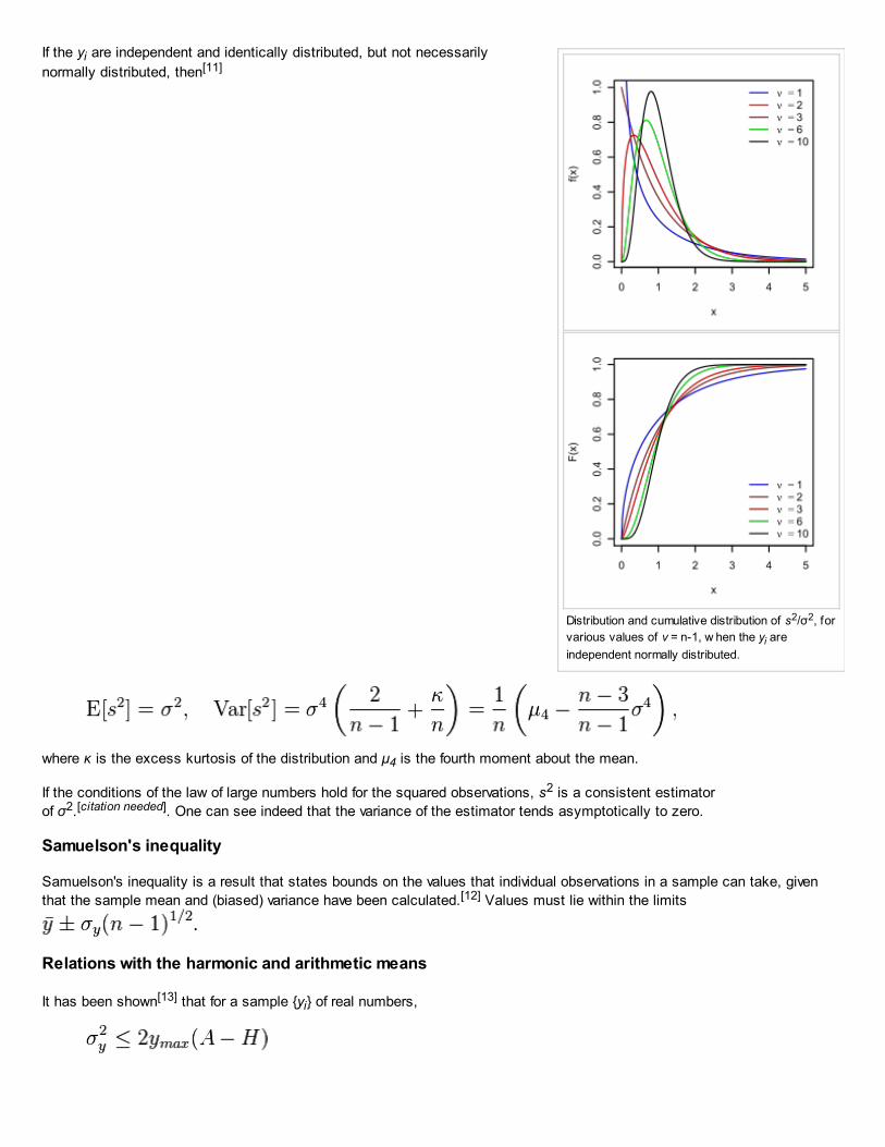
Distribution and cumulative distribution of s2/σ2, for

various values of ν = n-1, w hen the yi are

independent normally distributed.

If the yi are independent and identically distributed, but not necessarily

normally distributed, then[11]

where κ is the excess kurtosis of the distribution and μ4 is the fourth moment about the mean.

If the conditions of the law of large numbers hold for the squared observations, s2 is a consistent estimator

of σ2.[citation needed]. One can see indeed that the variance of the estimator tends asymptotically to zero.

Samuelson's inequality

Samuelson's inequality is a result that states bounds on the values that individual observations in a sample can take, given

that the sample mean and (biased) variance have been calculated.[12] Values must lie within the limits

Relations with the harmonic and arithmetic means

It has been shown[13] that for a sample {yi} of real numbers,

where ymax is the maximum of the sample, A is the arithmetic mean, H is the harmonic mean of the sample and is the

(biased) variance of the sample.

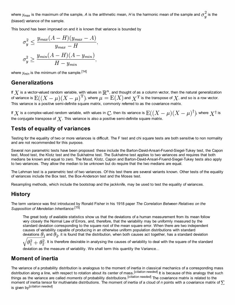
This bound has been improved on and it is known that variance is bounded by

where ymin is the minimum of the sample.[14]

Generalizations

If is a vector-valued random variable, with values in , and thought of as a column vector, then the natural generalization

of variance is , where and is the transpose of , and so is a row vector.

This variance is a positive semi-definite square matrix, commonly referred to as the covariance matrix.

If is a complex-valued random variable, with values in , then its variance is , where is

the conjugate transpose of . This variance is also a positive semi-definite square matrix.

Tests of equality of variances

Testing for the equality of two or more variances is difficult. The F test and chi square tests are both sensitive to non normalityand are not recommended for this purpose.

Several non parametric tests have been proposed: these include the Barton-David-Ansari-Fruend-Siegel-Tukey test, the Capontest, Mood test, the Klotz test and the Sukhatme test. The Sukhatme test applies to two variances and requires that bothmedians be known and equal to zero. The Mood, Klotz, Capon and Barton-David-Ansari-Fruend-Siegel-Tukey tests also applyto two variances. They allow the median to be unknown but do require that the two medians are equal.

The Lehman test is a parametric test of two variances. Of this test there are several variants known. Other tests of the equalityof variances include the Box test, the Box-Anderson test and the Moses test.

Resampling methods, which include the bootstrap and the jackknife, may be used to test the equality of variances.

History

The term variance was first introduced by Ronald Fisher in his 1918 paper The Correlation Between Relatives on the

Supposition of Mendelian Inheritance:[15]

The great body of available statistics show us that the deviations of a human measurement from its mean followvery closely the Normal Law of Errors, and, therefore, that the variability may be uniformly measured by thestandard deviation corresponding to the square root of the mean square error. When there are two independentcauses of variability capable of producing in an otherwise uniform population distributions with standarddeviations and , it is found that the distribution, when both causes act together, has a standard deviation

. It is therefore desirable in analysing the causes of variability to deal with the square of the standard

deviation as the measure of variability. We shall term this quantity the Variance...

Moment of inertia

The variance of a probability distribution is analogous to the moment of inertia in classical mechanics of a corresponding mass

distribution along a line, with respect to rotation about its center of mass.[citation needed] It is because of this analogy that such

things as the variance are called moments of probability distributions.[citation needed] The covariance matrix is related to themoment of inertia tensor for multivariate distributions. The moment of inertia of a cloud of n points with a covariance matrix of

is given by[citation needed]

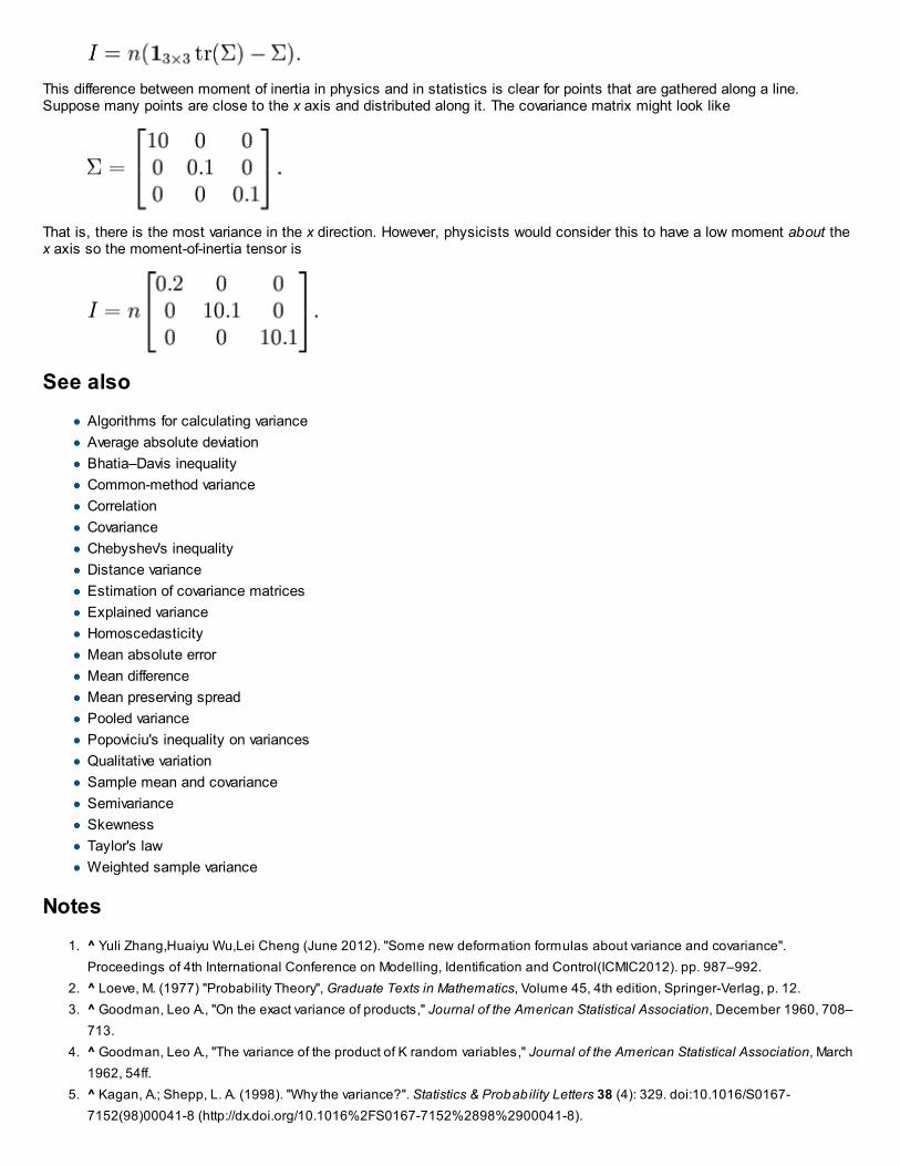
This difference between moment of inertia in physics and in statistics is clear for points that are gathered along a line.Suppose many points are close to the x axis and distributed along it. The covariance matrix might look like

That is, there is the most variance in the x direction. However, physicists would consider this to have a low moment about thex axis so the moment-of-inertia tensor is

See also

Algorithms for calculating variance

Average absolute deviation

Bhatia–Davis inequality

Common-method variance

Correlation

Covariance

Chebyshev's inequality

Distance variance

Estimation of covariance matrices

Explained variance

Homoscedasticity

Mean absolute error

Mean difference

Mean preserving spread

Pooled variance

Popoviciu's inequality on variances

Qualitative variation

Sample mean and covariance

Semivariance

Skewness

Taylor's law

Weighted sample variance

Notes

1. ^ Yuli Zhang,Huaiyu Wu,Lei Cheng (June 2012). "Some new deformation formulas about variance and covariance".

Proceedings of 4th International Conference on Modelling, Identification and Control(ICMIC2012). pp. 987–992.

2. ^ Loeve, M. (1977) "Probability Theory", Graduate Texts in Mathematics, Volume 45, 4th edition, Springer-Verlag, p. 12.

3. ^ Goodman, Leo A., "On the exact variance of products," Journal of the American Statistical Association, December 1960, 708–

713.

4. ^ Goodman, Leo A., "The variance of the product of K random variables," Journal of the American Statistical Association, March

1962, 54ff.

5. ^ Kagan, A.; Shepp, L. A. (1998). "Why the variance?". Statistics & Probability Letters 38 (4): 329. doi:10.1016/S0167-

7152(98)00041-8 (http://dx.doi.org/10.1016%2FS0167-7152%2898%2900041-8).

This page w as last modif ied on 23 October 2013 at 15:27.

Text is available under the Creative Commons Attribution-ShareAlike License; additional terms may apply. By

using this site, you agree to the Terms of Use and Privacy Policy.

Wikipedia® is a registered trademark of the Wikimedia Foundation, Inc., a non-profit organization.

6. ^ Johnson, Richard; Wichern, Dean (2001). Applied Multivariate Statistical Analysis. Prentice Hall. p. 76. ISBN 0-13-187715-1

7. ^ Navidi, William (2006) Statistics for Engineers and Scientists, McGraw-Hill, pg 14.

8. ^ Montgomery, D. C. and Runger, G. C. (1994) Applied statistics and probability for engineers, page 201. John Wiley & Sons

New York

9. ^ Knight K. (2000), Mathematical Statistics, Chapman and Hall, New York. (proposition 2.11)

10. ^ Casella and Berger (2002) Statistical Inference, Example 7.3.3, p. 331

11. ^ Neter, Wasserman, and Kutner (1990) Applied Linear Statistical Models, 3rd edition, pp. 622-623

12. ^ Samuelson, Paul (1968)"How Deviant Can You Be?", Journal of the American Statistical Association, 63, number 324

(December, 1968), pp. 1522–1525 JSTOR 2285901 (http://www.jstor.org/stable/2285901)

13. ^ Mercer A McD (2000) Bounds for A-G, A-H, G-H, and a family of inequalities of Ky Fan’s type, using a general method. J Math

Anal Appl 243, 163–173

14. ^ Sharma R (2008) Some more inequalities for arithmetic mean, harmonic mean and variance. J Math Inequalities 2 (1) 109–

114

15. ^ Ronald Fisher (1918) The correlation between relatives on the supposition of Mendelian Inheritance

(http://digital.library.adelaide.edu.au/dspace/bitstream/2440/15097/1/9.pdf)

Retrieved from "http://en.wikipedia.org/w/index.php?title=Variance&oldid=578415738"

Categories: Theory of probability distributions Statistical deviation and dispersion Data analysis