How Costly Are Debt Crises?

Davide Furceri and Aleksandra Zdzienicka

WP/11/280

© 2011 International Monetary Fund WP/11/280

IMF Working Paper

Middle East and Central Asia, and African Departments

How Costly Are Debt Crises?

Prepared by Davide Furceri and Aleksandra Zdzienicka1

Authorized for distribution by Joël Toujas-Bernaté and Hervé Joly

December 2011

Abstract

The aim of this paper is to assess the short- and medium-term impact of debt crises on GDP. Using an unbalanced panel of 154 countries from 1970 to 2008, the paper shows that debt crises produce significant and long-lasting output losses, reducing output by about 10 percent after eight years. The results also suggest that debt crises tend to be more detrimental than banking and currency crises. The significance of the results is robust to different specifications, identification and endogeneity checks, and datasets.

JEL Classification Numbers:G1, E6

Keywords: output losses, debt crises, sovereign defaults

Authors’ e-mail:dfurceri@imf.org; azdzienicka@imf.org.

1 The authors would like to thank Said Bakhache, Oscar Bajo, Adolfo Barajas, Charles Calomiris, Hervé Joly, Luiz de Mello, Markus Jorra,Yngve Lind, Keiichi Nakatani, Javier Perez, Jean-Luc Schneider, Carlo Sdralevich, Athanasios Tagkalakis, Joël Toujas-Bernaté , Dave Turner, Paul Van Den Noord, Luke Willard, and other participants to the OECD Economics Department Seminar, the XVIII Meeting in Public Economics, the 3rd EMG Conference for Emerging Markets Finance, the IMF-MCD and the IMF-RES Department Seminars for useful comments and discussions, and Kadia Kebet, Désirée Amon and Kia Penso for excellent editorial assistance.

This Working Paper should not be reported as representing the views of the IMF.

The views expressed in this Working Paper are those of the author(s) and do not necessarily represent those of the IMF or IMF policy. Working Papers describe research in progress by the author(s) and are published to elicit comments and to further debate.

2

I. INTRODUCTION

The recent general increase in public debt levels and severe funding pressures faced by some European countries has brought renewed attention to the problems of sovereign debt. Although it is a common view that debt crises may be detrimental and that large increases in public debt have frequently led to sovereign defaults, few studies have tested the effect of debt crises on output, and even fewer papers have focused on the timing of the recovery after debt crisis episodes.1

The economic literature has identified three main channels through which sovereign debt crises affect output.2 The first channel is through the exclusion from international capital markets. Gelos et al. (2011) show that after a sovereign default, countries were excluded from international capital markets for about four years on average. Similarly, Richmond and Dias (2008) find that exclusion from international capital markets after a sovereign default lasted on average 4 years: 5.5 years for debt crisis episodes in the 1980s, 4.1 years in the 1990s, and 2.5 years in the 2000s. The second channel is through an increase in the cost of borrowing. For example, Borensztein and Panizza (2009) find that for 31 emerging market economies in the period 1997–2004, in the year after a sovereign default episode spreads increased by about 400 basis points compared to tranquil times. The third channel is through international trade. Rose (2005) finds a significant reduction in bilateral trade of approximately 8 percent per year following the occurrence of a sovereign default. In addition to these channels, debt crises can affect output indirectly by leading to banking and currency crises (De Paoli et al. 2009), and through domestic channels such as a reduction in consumption and investment or fall in total factor productivity.

The results of the empirical literature on the relation between sovereign default and growth have in general confirmed that debt crises may lead to significant output contractions. Sturzenegger (2004), using cross-country and panel regressions, finds that debt defaults are associated with a reduction in output growth of about 0.6–2.2 percentage points. Similarly, Borensztein and Panizza (2010) find that defaults are associated with a decrease in growth of 1.2 percentage points per year. De Paoli et al. (2009), comparing output growth five years before and after the occurrence of a debt crisis, find that debt crises are associated with large output losses of at least 5 percent per year. In contrast, Levy-Yeyati and Panizza (2011), analyzing quarterly data for

1 Cerra and Saxena (2008) Panizza et al., (2009).

2 See Panizza et al. (2009) for a survey of the recent literature on sovereign debt defaults, its determinants and effects.

3

output growth, find that growth recovers in the quarters immediately after the occurrence of a debt crisis.3

However, the results of these growth regressions should be interpreted with some caution because they may suffer from two main biases. First, sovereign debt crises may be endogenous to output contractions. Indeed, many episodes of debt defaults have occurred in periods of strong output contractions. Chiang and Coronado (2005), and Borensztein and Panizza (2010) attempt to address this issue by using a two-step approach in which the probability of sovereign defaults is estimated in the first-stage regression, and then used as a regressor in the second stage in the growth regression. However, this approach does not fully address endogeneity problems given the impossibility of finding true strongly exogenous instruments for debt crises. In addition, the results of the second stage regression may be very sensitive to the particular model used to estimate the probabilities of debt crises.

The second form of bias comes from the indistinguishable connection that exists between currency, banking, and debt crises. This is particularly the case for emerging economies simultaneously hit by all three. The simultaneous occurrence of these types of financial crisis is often attributed to the so-called “original sin” syndrome (Eichengreen et al., 2003), taking place when most of the private and public debt is short-term and/or denominated in foreign currency. Following large domestic exchange rate depreciations associated with currency crises, public debt (when mostly foreign currency denominated) can increase considerably and lead to defaults. Reinhart and Rogoff (2010a, b) suggest the following causality: private-sector defaults precede banking sector crises that coincide with or precede public debt defaults. At the same time, the opposite may also occur: public debt defaults may lead to banking crises when banks are the main holders of government debt. Banking and debt crises could also lead to currency crises. For instance, third-generation crisis theory (Krugman, 1999) underlines the role of maturity mismatches and currency disequilibria in private (mostly banking-sector) balance sheets as the main reason for the onset of currency crises.

This paper tries to address these issues. In particular, its contribution to the existing literature is fourfold:

It analyzes the impact of debt crises on output in both the short term and the medium term.

It attempts to address endogeneity and reverse causality by using two approaches. The first, in line with the most recent empirical literature that analyzes the determinants of growth in a panel framework, consists of using a two-step GMM-system estimator. The

3 The authors argue that a more persistent impact of sovereign default, found using annual data. is likely to be driven by the anticipation of defaults. Panizza et al. (2009), comparing the impact of anticipated and non-anticipated defaults on output, find no significant differences between the two types of crises.

4

second approach consists of estimating the impact of debt crises on growth using the two-step GMM only for those debt crises episodes that occurred in periods of relatively good economic performance.

It tries to isolate the impact of debt crises from the effect of banking and currency crises using two different estimation strategies. The first approach consists of estimating the effect of debt crises on output together with the effect of currency and banking crises. In this way, it is possible to quantify the marginal contribution of each crisis to output. In the second strategy, the effect of debt crises on output is estimated only for those episodes for which neither a banking nor a currency crisis occurred in the two years before, during, or the two years after the onset of a debt crisis.

To check the robustness of our results, several datasets of starting dates for debt crisis episodes are used.

The estimates, based on an unbalanced panel of 154 countries from 1970 to 2008, suggest that debt crises are very costly to output in both the short term and the medium term. In the short term, the results suggest that debt crises reduce contemporaneous output growth by about 6 percentage points. The results are robust to different specifications, and to different robustness checks to control for endogeneity and identification of debt crises (vs. banking and currency crises). In particular, focusing on those debt crisis episodes characterized by contemporaneous favorable economic performance, the analysis suggests that debt crises reduce contemporaneous output growth by about 6-10 percentage points. Similarly, focusing on debt crisis episodes for which neither a banking nor a currency crisis occurred in the two years before, during, or after the onset of a debt crisis, the results confirm that debt crises significantly and negatively affect contemporaneous output growth, with a magnitude of the effect of about 8 percentage points. The results are also robust to alternative datasets with a magnitude of the effect ranging from 5 to 10 percentage points.

Debt crises are also associated with significant output losses over the medium term: eight years after the occurrence of a debt crisis, output contracts by about 10 percent (compared to the country-specific output trend). The statistical significance of the result is robust to the estimation procedures used (local projections and ARDL) and to different specifications.

Finally, the paper presents empirical evidence that output growth is reduced not only when a debt crisis occurs, but also when public (total and foreign) debt exceeds a given threshold.

The rest of the paper is organized as follows: Section 2 describes the data and the identification of debt crisis episodes. Section 3 presents the empirical methodology used to assess the short- and medium-term effects of debt crises on output, and the results. Section 4 summarizes the main results and concludes with some issues for future research.

5

II. DATA

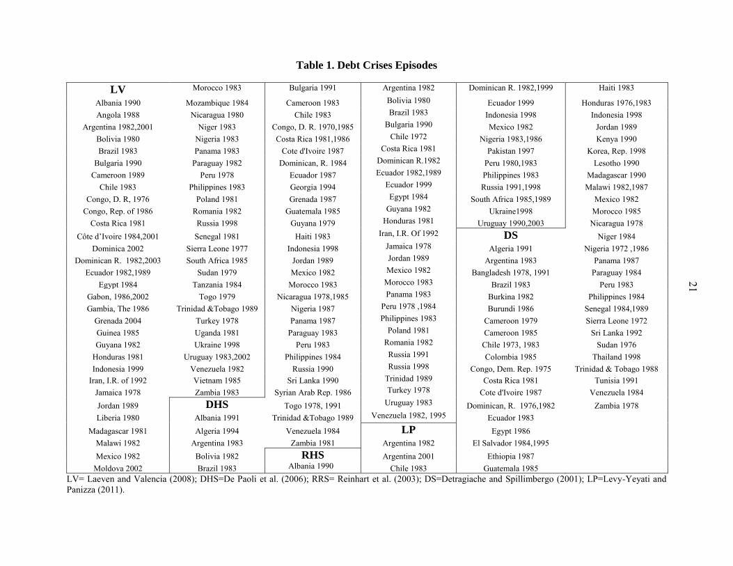
To identify debt crisis episodes the paper relies on several datasets (Table 1):

The first dataset is the one constructed by Laeven and Valencia (2008) who list the starting date of debt crisis episodes as a compilation of years of sovereign defaults to private lending (creditors) and years of debt rescheduling. The authors rely on information from Beim and Calomiris (2001), World Bank (2002), Sturzenegger and Zettelmeyer (2006), and IMF Staff Reports.4 Overall the authors identify 63 crisis episodes, which mainly occurred in the 1980s: seven episodes occurred in the period 1970–1979, 41 between 1980 and 1989, seven in the period 1990–1999, and eight after 1999.

The second set of debt crisis episodes is the one collected by De Paoli et al. (2006). The authors identify 39 episodes of sovereign default over the 1970–2000 period, in which the arrears on principal on external obligations to private creditors reached at least 15 percent of total commercial debt outstanding and/or there was a rescheduling with private creditors as listed in the World Bank’s Global Development Finance.

An alternative dataset of debt crisis episodes is the one constructed by Reinhart et al. (2003). The authors identify 31 debt crisis episodes over the period 1970–2001 using the dates reported in Beim and Calomiris (2001) on defaults and restructurings, and Standard and Poor’s Credit Week information.

A fourth dataset is Detragiache and Spillimbergo (2001) which covers 54 episodes of debt crisis. Defaults are identified when arrears of principal on external obligations to commercial creditors exceed 5 percent of total commercial debt outstanding (excluding the episodes that occur within four years of the previous defaults) and/or there is a rescheduling with private creditors as listed in the World Bank’s Global Development

Finance.

Finally, the last dataset considered in the analysis is Levy-Yeyati and Panizza (2011). The authors identify 20 default episodes over the period 1980–2003 (excluding the episodes that occured within three years of the previous defaults). Episodes are classified as beginning years of foreign currency bank or bond debt default, using information reported in Standard and Poor’s Credit Week, the World Bank’s Global Development

Finance, and the financial press.

4 The World Bank Global Development Finance Report (2002) provides a list of 26 countries for which debt-restructuring agreements with their commercial creditors were completed in 2001. Beim and Calomiris (2001) provide the date of debt defaults for several emerging economies during the period 1970–2000. Sturzenegger and Zettelmeyer (2006) list selected government defaults and restructurings of privately held bonds and loans over the period 1920–2004.

6

Table 2 presents descriptive statistics for total and foreign public debt (as share of GDP), and GDP growth in relation to the debt crisis episodes identified in the datasets described above. Looking at the table, it is immediately evident that starting dates of debt crises are associated with periods of negative growth and relatively high domestic and foreign public debt. In particular, focusing on the first row of the table (for which more episodes and more observations for public debt are available), it appears that on average, at the time of debt crises, the gross public debt-to-GDP ratio is about 80 percent, the public foreign gross debt-to-GDP ratio is about 55 percent, and GDP growth is about –2 percent. There is, however, considerable dispersion around these averages.

Data for banking and currency crises episodes are taken from Laeven and Valencia (2008). The authors determine the starting dates of banking crises by combining quantitative indicators measuring banking sector distress, such as a sharp increase in nonperforming loans and bank runs, with a subjective assessment of the situation. In particular, the database extends and builds on the Caprio et al. (2005) banking crisis database and covers the universe of systemic banking crises for the period 1970–2007. Currency crisis episodes are identified as episodes of nominal depreciation of the currency of at least 30 percent that is also at least a 10 percent increase in the rate of depreciation compared to the year before. Data for real GDP are taken from the World Bank Economic Indicators. Data for public (domestic and foreign5) debt are taken from Panizza (2008).

III. EMPIRICAL ANALYSIS

This section analyzes the impact of debt crises on short-term growth. The first part of the section assesses the short-term effect of debt crises controlling for reverse causality, identification of debt crises (vs. banking and currency crises) and providing several robustness checks. Additionally, it investigates the impact of the (total and foreign) public debt-to-GDP ratio on output and the existence of debt thresholds. The second part of the section extends the analysis to the medium-term, analyzing the response of output up to 8 years after the occurrence of a debt crisis.

A. Short Term

Following previous studies in the literature on the short-term effects of banking and/or currency crises on output, the methodological approach used in the paper consists of estimating contemporaneous output growth against a dummy variable that takes a value equal to 1 for the occurrence of a crisis and 0 otherwise, and a set of variables influencing short-term growth. In particular, the formal specification of the empirical model used for the short-term analysis is as follows:

5 Foreign debt is defined as public debt issued in foreign countries and under the jurisdiction of a foreign court.

7

(1)

where is the log of real GDP for country i at time t and zero otherwise, is a dummy

variable that takes the value equal to 1 if a debt crisis occurred in country i at time t and 0 otherwise, are country-specific effects included to account for different growth trends among countries, is a set of variables influencing growth in the short-term, and represents the marginal effect of the occurrence of a debt crisis on growth. The empirical literature on growth has suggested numerous variables as possible determinants of growth (see, for example, Levine and Renelt, 1992; Sala-i-Martin 1997, Sala-i-Martin et al. 2004). However, some of these variables are likely to influence growth only over the medium term, and are not available on a yearly basis (e.g., human capital) over a long time span and for a large set of countries. Therefore to keep the specification parsimonious, the variables included in the vector X have been restricted to: trade openness (defined as the share of total exports and imports in GDP), population growth, (private) credit growth, real exchange rate growth and the initial (lagged) level of GDP. In addition, as the main concern is to introduce relevant control variables into the regression so that their omission does not bias the estimated impact of a debt crisis on output, two lags of real GDP growth have been included.

To address endogeneity due to the presence of the lagged dependent variable among regressors and to reverse causality from growth to the occurrence of debt crises, Equation 1 has been estimated using the two-step GMM-system estimator. 6

The results obtained estimating Equation 1 (column I, Table 3) suggest that debt crises significantly reduce contemporaneous output growth by about 6 percentage points. The significance of the results is robust across the different specifications with an estimated impact that ranges from about 5 to 6 percentage points (columns II–VII, Table 3). The control variables that have a positive and (most of the time) statistically significant effect are trade openness, population growth, credit growth and the first lag of real GDP growth.

Consistency of the two-step GMM estimates has been checked using the Hansen and the Arellano-Bond tests. The Hansen J-test of over-identifying restrictions, which tests the overall validity of the instruments by analyzing the sample analog of the moment conditions used in the estimation process, cannot reject the null hypothesis that the full set of orthogonality conditions are valid (across the different specifications the p-value ranges from 0.3 to 1). The Arellano-Bond test for autocorrelation cannot reject the null hypothesis of no second-order serial

6 The two-step GMM-system estimates (with Windmeijer standard errors) are computed using the xtabond2 Stata command developed by Roodman (2009a). Openness, lagged real exchange rate growth, lagged real credit growth, lagged credit growth, and lagged debt crises are as predetermined; other control variables are considered as endogenous (instrumented using up to 3 lags). The significance of the results is robust to different choices of instruments and predetermined variables.

8

correlation in the first-differenced error terms (across the different specifications the p-value ranges from 0.2 to 1). However, as pointed out by Roodman (2009b) a problem with applying the GMM-system estimator is that it may generate too many instruments, which may reduce the efficiency of the two-step estimator and weaken the Hansen test of the instrument’s joint validity. While it is common practice to limit the number of instruments so that they do not exceed the number of panels (as in our case7), there is no precise guidance on what is the appropriate number of instruments. To address this issue and check the robustness of our results, we follow Roodman’s suggestions: i) include the difference-Hansen-test, ii) collapse the number of instruments and iii) check the validity of the results using the GMM-difference estimator. The results presented in Table 4 confirm the robustness of our results and validate the evidence of a negative and statistically significant impact of debt crises on growth.

Although these tests confirm the consistency of the GMM estimates, reverse causality from growth to debt crises may still be an issue because, as shown in Table 2, debt crises tend to occur in periods of negative growth, and because of the impossibility of finding true strongly exogenous instruments. To address this issue and to check the robustness of the results, Equation 1 has been re-estimated excluding those debt crisis episodes that occurred in periods when contemporaneous output fell after a period of positive growth (growtht<0, growtht-1>0). In detail, two different specifications are estimated. In the first specification all observations are considered. In the second specification, the observations characterized by contemporaneous negative growth and the occurrence of a debt crisis are dropped. The results obtained with both approaches confirm that debt crises have a statistically significant and negative impact on contemporaneous output growth (Column II and III, Table 5). In addition, given that debt crises also tend to occur in periods of positive growth (Table 2), we re-estimated Equation 1, focusing only on debt crisis episodes that occurred in periods of contemporaneous and lagged positive output gap (measured as the deviation of real GDP from its trend) ,8 and in periods when contemporaneous growth did not slow down. The results in this case also point to a significant and negative effect of debt crises on growth of 7.5 percent for periods of output gap (Column IV, Table 5) and 9.3 percent for periods of non-slowing growth (Column V, Table 5). However, it must be stressed that these results may not be fully comparable with those presented in the baseline, because the selection mechanism of the debt crises focuses on those countries that defaulted in relatively good times. These defaults may be viewed as inexcusable in terms of Grossman and Huyck (1988) and thus may be punished more harshly punished. This could explain the larger default costs resulting from this approach.9 Nevertheless, despite this limitation, we believe that this approach represents a useful robustness check.

7 We have 118 instruments for 154 panels.

8 Trend GDP is estimated using an HP filter with a smoothness parameter equal to 100.

9 We are grateful to an anonymous referee for making this point.

9

To further check the robustness of the results, another approach to addressing reverse causality from growth to debt crises has also been carried out. Following Chiang and Coronado (2005), and Borensztein and Panizza (2009), the approach consists of estimating the probability of default using various predictors of debt crises, and then using the predicted probability of default as a regressor in the growth regression.10 The results obtained with this approach, not reported, confirm that debt crises have a significant and negative effect on contemporaneous output growth. The magnitude of the effect, however, is very sensitive to the choice of specification used to estimate default probabilities, with point estimates that range from 1 to 25 percentage points.

Comparison with Previous Studies and Robustness Checks

The results of the baseline regression suggest that debt crises reduce contemporaneous output growth by about 6 percentage points. While the size of the estimated coefficient is higher than the one reported in some of the previous studies (e.g. Sturzenegger, 2004; Borensztein and Panizza, 2010; and Levy-Yeyati and Panizza, 2011) the difference in the point estimate is not statistically significant. 11

However, to further explore the robustness of our results, also in comparison with previous studies, three robustness checks have been carried out. First, equation 1 has been re-estimated using the alternative datasets described in Section 2. The results reported in Table 6 provide robust empirical evidence that debt crises have a significant and negative effect on contemporaneous output, with point estimates ranging from 5 to 10 percentage points. Since these datasets mainly differ in the composition of the countries to which a debt crisis is attributed, rather than in the dating of the crisis itself, it is likely that the different estimates simply reflect the heterogeneous response of countries to the debt crises and the different severities of the crises. However, these differences are not statistically significant.

Second, to control for differences in the set of explanatory variables used in the empirical analysis and to check for possible omission bias, a measure of terms of trade and the investment-to-GDP ratio have been included in the analysis. However, while these additional variables turn out to be statistically insignificant, the estimated effect of debt crises on growth changes only slightly and not in a statistically significant manner (Table 7).

10 The probability of default is estimated using a logit model and considering as explanatory variables: i) the debt-to-GDP ratio; ii) banking crisis dummy; iii) currency crisis dummy; iv) contemporaneous and lagged growth; v) the ratio of foreign reserve to GDP; vi) the ratio of short-term debt to GDP ; vii) openness; ix) exchange rate volatility and x) inflation. The full set of results is available upon request.

11 We cannot reject the hypothesis that the estimated coefficient in the baseline is statistically different from the lowest point estimate (0.6) found in previous studies (Sturzenegger, 2004).

10

Third, to control for differences in the econometric specification, Equation 1 has been re-estimated using OLS as in Sturzenegger (2004), Borensztein and Panizza (2010), and Levy-Yeyati and Panizza (2011). The result with this approach points to a lower impact of debt crises on growth, although the difference is not statistically significant (Table 7). These robustness checks corroborate the validity of our results.

Debt crises versus currency and banking crises

The close connection between currency, banking, and debt crises makes it particularly difficult to isolate the impact of debt crises on real output. For example, as pointed out by Reinhart and Rogoff (2010b), it is possible that a banking (and/or currency) crisis may trigger a debt crisis, in which case the estimated effect of debt crises on contemporaneous output growth could be just interpreted as the lagged effect of banking (or currency) crisis episodes. To address this issue, two different approaches have been taken.

The first approach consists of estimating the effect of debt crises on output together with the effect of currency and banking crises. In this way, it is possible to quantify the marginal contribution of each crisis to output. For this purpose the following specification is estimated:

(2)

where (

is a dummy variable that takes the value equal to 1 if a currency (banking) crisis occurred in country i at time t, and zero otherwise. The (full) empirical specification includes three types of twin crises: debt-currency (

debt-banking

, and currency-banking

(

). Similarly to Hutchinson and Noy (2005), twin crises are defined as those crises in which the onset of a given crisis occurs two years before, during, or two years after the onset of another type of crisis. Finally, Equation 3 also includes triple debt-currency-banking crises

. Triple crises are defined as those crises in which the onset of a given crisis occurs two years before, during, or two years after the onset of the other two types of crises. The coefficients represent the marginal effect of debt, currency, banking, twin, and triple crises on output growth. Thus, if the ( coefficients are found to be negative and statistically significant, it implies that the occurrence of a twin (triple) crisis has an additional negative impact on output growth above and beyond the combined effect of the two (three) types of crises. The results obtained estimating Equation 3 (Table 8) confirm that debt crises significantly reduce output growth with an estimated impact that ranges across the different specifications from 5 to 8 percentage points (Column I-IV, Table 8). More interestingly, looking at the full specification, the effect of debt crises seems to be more detrimental than the effect of currency or banking crises. Among the twin and the triple crisis dummies, only the twin banking-currency crisis dummy has a negative and statistically significant effect. The results are qualitatively robust to different year windows (one year and three years).

11

The second approach consists of estimating the effect of debt crises on output together with the effect of currency and banking crises but only for those episodes for which neither a banking nor a currency crisis occurred in the two years before, during, or the two years after the onset of a debt crisis. By doing this, the number of debt crises episodes is reduced to 20. The results obtained with this approach confirm that debt crises significantly reduce output growth (Column V of Table 8). In particular, the occurrence of a debt crisis, neither preceded nor followed by a banking and/or a currency crisis, is found to reduce contemporaneous output growth by about 8 percentage points.

Debt thresholds

The results presented in the previous section have provided strong empirical evidence that debt crises significantly reduce contemporaneous output growth. Another interesting hypothesis to test is whether output growth is reduced not only when a debt crisis occurs, but also when public (total and foreign) debt exceeds a particular threshold. A first work in this direction is Reinhart and Rogoff (2010a). The authors, analyzing a multi-country historical large dataset on central government debt as well as data on external (public and private) debt, present descriptive evidence showing that when the gross public debt-to-GDP ratio exceeds 90 percent, median growth rates fall by one percentage point. Similarly, annual growth declines by about 2 percentage points when external debt reaches 60 percent of GDP.

To test Reinhart and Rogoff’s predictions a model specification similar to Equation 1 has been estimated alternatively, using the debt-to-GDP ratio (foreign debt-to-GDP) and a dummy variable taking a value equal to 1 if the gross debt-to-GDP (foreign debt-to-GDP) ratio exceeds a given threshold and zero otherwise. Table 9 displays the results obtained for the linear and nonlinear effects of debt on output growth. Starting with the debt-to-GDP ratio (Columns I-IV), the results provide no statistical evidence of a linear relationship between growth and debt, and show that output is reduced by about 1.8 percentage points when the debt-to-GDP ratio exceeds 70 percent. Lower thresholds, tested but not reported, are found to be not statistically significant, while the 80 and 90 percent thresholds are associated with a decline in output growth greater than 2 percentage points. Similarly, higher thresholds are found not to contribute significantly to additional negative effects. This finding is consistent with the evidence provided in recent studies (Kumar and Woo, 2010; Checherita and Rother, 2010; and Carner et al. 2010).

The results for the foreign debt-to-GDP ratio provide only weak statistical evidence of a linear relationship between foreign debt and output growth, and show that output growth is reduced by about 2.4 percentage points when the ratio exceeds 80 percent. Lower thresholds, such as 60 and 70 percent, are not statistically significant at 5 percent. Similarly, higher thresholds are found to not contribute significantly to additional negative effects.

Overall, the results seems to validate Reinhart and Rogoff’s predictions (i.e., the existence of thresholds for the debt-to-GDP ratio and the foreign debt-to-GDP ratio above which output growth starts to decline), although not in terms of the magnitude of these effects.

12

The analysis also suggests that the effect of high (total and foreign) debt is considerably lower than the effect of debt crises, which indirectly implies that a large debt burden is not the only channel through which debt crises negatively affect output. This finding is confirmed from the results obtained when threshold and debt crisis dummies are jointly included in the estimation. In particular, both dummies are statistically significant, but while debt crises reduce output by about 45 percentage points, higher debt levels (total and foreign) reduce output by about 1.5–2 percentage points.

B. Medium Term

This paper also assesses whether the effect of debt crises on output is reversed over the medium term. In order to estimate the medium-term dynamic impact of debt crisis episodes on output, the paper follows the method proposed by Jorda (2005) and Teuling and Zubanov (2010), which consists of estimating impulse response functions (IRFs) directly from local projections. In detail, for each future period k the following equation has been estimated on annual data:

(3)

where k = 1, ...8, are country fixed effects, Timeit are country-specific time trends, and

measures the impact of debt crises on the change of (the log of) the real output for each future period k.12 The number of lags (l) has been chosen to be equal 2, even if the results are extremely robust to different numbers of lags included in the specification. Corrections for heteroskedasticity, when appropriate, have been applied using White robust standard errors. IRFs are then obtained by plotting the estimated for k = 0, 1, …8, with 95 percent confidence bands for the estimated IRFs computed using the standard deviations associated with the estimated coefficients . While the presence of a lagged dependent variable and country fixed effects may in principle bias the estimation of

and in small samples (Nickel, 1981), the length of the time dimension mitigates this concern.13

The results from estimating the medium-term impact of debt crises on output using Equation 3 are presented in Figure 1. The figure suggests that debt crises have long-lasting effects, reducing output even eight years after the occurrence of the crisis. In particular, the estimates suggest that eight years after the occurrence of a debt crisis output is lower by about 10 percent.

To check the robustness of our results, Equation 3 has been re-estimated by alternatively including a common time trend and time fixed effects (Panels A and B, Figure 2). The results using these different controls remain statistically significant and broadly unchanged.

12 Since fixed effects are included in the regression the dynamic impact of debt crises on output should be interpreted as changes in output compared to a baseline country-specific output trend. 13 The finite sample bias is in the order of 1/T, where T in our sample is 39.

13

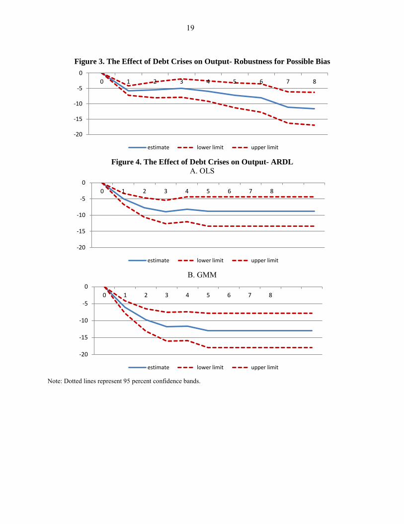
As shown by Teulings and Zubanov (2010), a possible bias from estimating Equation 3 using country fixed effects is that the error term of the equation may have a non-zero expected value, due to the interaction of fixed effects and country-specific arrival rates of crises. This would lead to a bias of the estimates that is function of k. To address this issue and check the robustness of our results, Equation 3 has been re-estimated by excluding country fixed effects from the analysis. The results reported in Figure 3, however, suggest that this bias is negligible (the difference in the point estimate is small and not statistically significant) and confirm the empirical evidence that eight years after the occurrence of a debt crisis, output is lower by about 10 percent.

As an additional robustness test the medium-term impact of debt crises on output has been re-estimated using an ARDL (4, 4) equation.14

(4)

The RFs are obtained by simulating a one-year crisis and by computing the response of output over time through the estimated coefficients. Confidence bands at 95 percent significance level are derived using Monte Carlo simulations in one thousand trials. The results obtained estimating Equation 4 with both OLS and GMM confirm that debt crises have long-lasting effects on output: eight years after the occurrence of a debt crisis output is lower by about 9–12 percent (Figure 4).

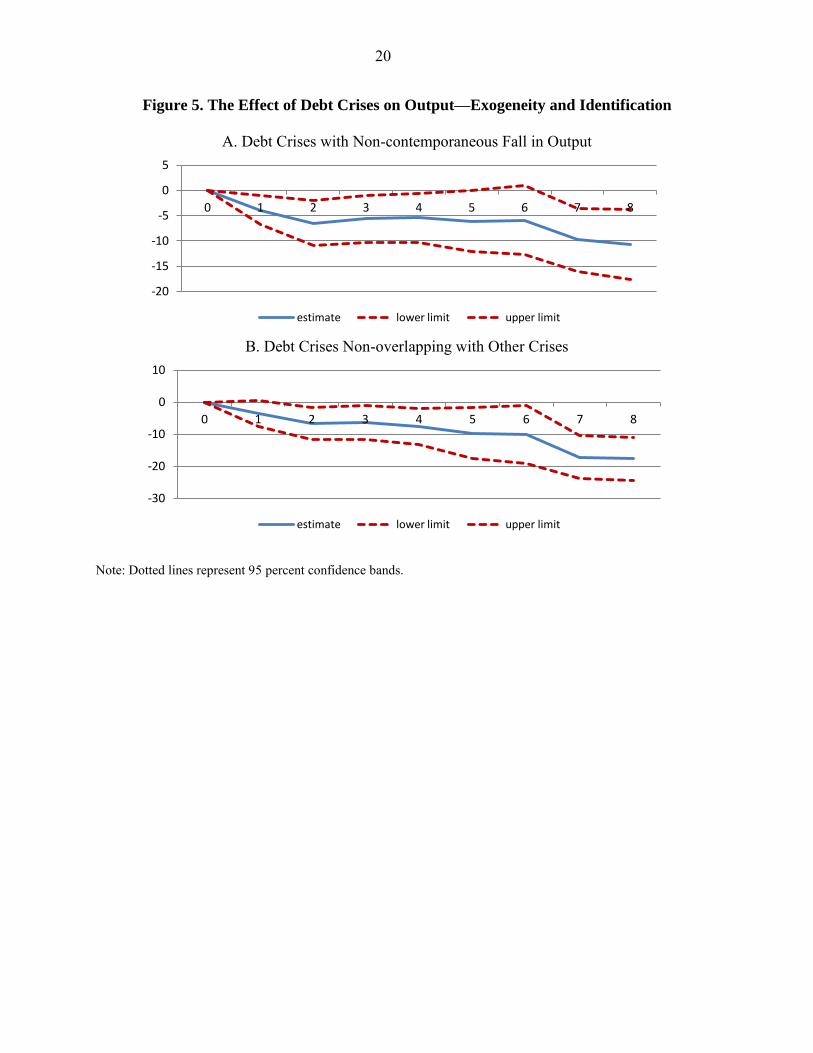
Finally, in order to address possible reverse causality15 and the identification problems discussed in the previous section, Equation 3 has been re-estimated by alternatively considering: (i) those debt crisis episodes with contemporaneous non-negative growth; (ii) debt crisis episodes for which neither a banking nor a currency crisis occurred in the eight years before, during, or in the eight years after the onset of a debt crisis. The results for these two cases are shown in Panels A and B of Figure 5, and corroborate the negative impact of debt crises on output over the medium term.

14 The approach was initially proposed by Romer and Romer (1989) and then recently applied by Cerra and Saxena (2008), Furceri and Mourougane (2009), and Furceri and Zdzienicka (2011) to assess the long-term impact of banking crises on economic activity. It is worth stressing that the IRFs derived using this approach may suffer from some problems, such as (i) they may be sensitive to the choice of the number of lags, which makes the IRFs less stable; (ii) the significance of long-lasting effects on output can be simply driven by the use of one-type-of-shock models (Cai and Den Haan, 2009); and iii) medium-term effects are more sensitive to endogeneity problems, because they are implicitly derived by estimating contemporaneous output growth.

15 In this approach the risk of reverse causality between changes in (the log of) output and the occurrence of a debt crisis is quite small, because changes in output are estimated for subsequent periods (from t +1 to t + 8). This is particularly the case for the estimates of the medium-term effect (i.e., eight years after the occurrence of a debt crisis).

14

IV. CONCLUSIONS AND ISSUES FOR FUTURE RESEARCH

The paper analyzes the short- and medium-run effects of debt crises on output for an unbalanced panel of 154 countries from 1970 to 2008. The results suggest that in the short term debt crises are very detrimental, reducing contemporaneous output growth by 6 percentage points. The results are robust to different specifications, and to different robustness checks to control for endogeneity and identification of debt crises (vs. banking and currency crises). In particular, focusing on those debt crisis episodes characterized by contemporaneous relatively good economic performance, the analysis suggests that debt crises reduce output growth by about 6–10 percentage points. Similarly, focusing on debt crisis episodes for which neither a banking nor a currency crisis occurred in the two years before, during, or the two years after the onset of a debt crisis, the results confirm that debt crises significantly and negatively affect contemporaneous output growth, with a magnitude of the effect of about 8 percentage points. The results are also robust to alternative datasets with a magnitude of the effect ranging from 5 to 10 percentage points. Since these datasets mainly differ in the composition of the countries to which a debt crisis is attributed, rather than in the dating of the crisis itself, it is likely that the different estimates simply reflect the heterogeneous response of countries to the debt crises and the different severities of the crises. These differences are, however, not statistically significant.

The medium-term analysis confirms the negative effect of debt crises on output. In particular, debt crises are associated with persistent output losses: eight years after the occurrence of a debt crisis, output is lower by about 10 percent. The statistical significance of the result is robust to the estimation procedures used (local projections and ARDL) and to different specifications. These are large estimates and should alarm policy makers about the risks of defaults.

Our study suggests that a number of interesting extensions can be pursued. First, as suggested by the results obtained by using different datasets, the response of output to debt crises may vary across countries and debt crisis episodes. Therefore, it would be useful to empirically examine the determinants of this heterogeneity, also differentiating between episodes of debt versus flow restructuring , and episodes that have involved preemptive/voluntary debt exchanges with private creditors before running arrears or outright default.

An additional promising direction would be to expand the investigation on whether output is negatively affected not only by the occurrence of a debt crisis, but to whether it is negatively affected when public (total and foreign) debt exceeds a particular threshold. The results presented in the paper suggest that output growth declines by about 1.8 percentage points (2.4 percentage points) when the gross debt-to-GDP ratio (foreign debt-to-GDP ratio) exceeds 70 (80) percent. This analysis could be extended by analyzing thresholds with non-parametric (or semi-parametric) approaches, and by looking at possible interactions between the share of public (total and foreign) debt and other variables such as trade openness, domestic saving, financial integration, financial development, and measures of perceived country risks.

15

REFERENCES

Beim, D. and C. Calomiris, 2001, Emerging Financial Markets, Appendix to Chapter 1 (New York: McGraw-Hill/Irwin Publishers).

Borensztein, E., and U. Panizza, 2009, “The Costs of Sovereign Default,” Staff Papers, International Monetary Fund, Vol. 56(4), pp. 683-741.

Cai, X., and W. J. Den Haan, 2009, “Predicting Recoveries and the Importance of Using Enough Information,” CEPR Discussion Paper No. 7508 (London: Centre for Economic Policy Research).

Caprio, G., and others, 2005, “Appendix: Banking Crisis Database,” in Systemic Financial

Crises: Containment and Resolution, ed. by Patrick Honohan and Luc Laeven (Cambridge, U.K.: Cambridge University Press).

Carner, M, T. Grennes, and F. Koeheler-Geib, 2010, “Finding the Tipping Point When Sovereign Debt Turns Bad,” Policy Research Working Paper No. 5391 (Washington: World Bank).

Cerra, V., and S. Saxena, 2008, “Growth Dynamics: The Myth of Economic Recovery,” American Economic Review, Vol. 98, pp. 439-57.

Checherita, C., and P. Rother, 2010, “The Impact of High and Growing Government Debt on Economic Growth: An Empirical Investigation for the Euro Area” ECB Working Papers

forthcoming.

Chiang, G., and J. Coronado, 2005, “A Two Step Approach to Assess the Cost of Default for Latin America,” www.urrutiaelejalde.org/Summer-School/2005/papers/coronadochiang.pdf.

De Paoli, B., G. Hoggarth, and V. Saporta, 2006, “Costs of Sovereign Defaults,” Bank of England Financial Stability Paper No. 1, July.

De Paoli, B., G. Hoggarth, and V. Saporta, 2009, “Output Costs of Sovereign Crises: Some Empirical Estimates,” Bank of England Working Paper No. 362.

Detragiache E., and A. Spilimbergo, 2001, “Crises and Liquidity–Evidence and Interpretation,” IMF Working Papers 01/2 (Washington: International Monetary Fund).

Eichengreen, B., R Hausmann, and U. Panizza, 2003, “Currency Mismatches, Debt Intolerance, and Original Sin: Why They Are Not the Same and Why It Matters,” NBER Working Paper No. 10036 (Cambridge, Massachusetts: National Bureau of Economic Research).

16

Furceri, D., and A. Mourougane 2009, “The Effect of Financial Crises on Potential Output: New Empirical Evidence form OECD Countries,” OECD Working Paper No. 699 (Paris: Organisation for Economic Co-operation and Development).

Furceri, D., and A. Zdzienicka, 2011, “The Real Effects of Financial Crises in the European Transition Economies,” Economics of Transition,17, 1-25.

G. Gelos, R. Sahay, and G. Sandleris, 2011, “Sovereign Borrowing by Developing Countries: What Determines Market Access?” Journal of International Economics, Vol. 83(2), pp 243-54.

Grossman, H. I. and J. B. Huyck, 1988, “Sovereign Debt as a Contingent Claim: Excusable Default, Repudiation, and Reputation,” The American Economic Review, Vol. 78 (5), pp 1088-97.

Hutchison, M., and N. Ilan, 2005, “How Bad Are Twins? Output Costs of Currency and Banking Crises,” Journal of Money, Credit and Banking, Vol. 37(4), pp. 725-52.

Jorda, O., 2005, “Estimation and Inference of Impulse Responses by Local Projections,” American Economic Review, Vol. 95, No. 1, pp. 161–82.

Krugman, P., 1999, “Balance Sheets, the Transfer Problem, and Financial Crises,” International

Tax and Public Finance, Springer, Vol. 6(4), pp. 459-72.

Kumar, M.S., and J.Woo, 2010, “Public Debt and Growth,” IMF Working Paper 10/174 (Washington: International Monetary Fund).

Leaven, L., and F. Valencia, 2008, “Systemic Banking Crises: a New Database,” IMF Working Paper 08/224 (Washington: International Monetary Fund).

Levine, R., and D. Renelt, 1992, “A Sensitivity Analysis of Cross-country Growth Regressions,” American Economic Review, Vol. 82, pp. 942–4.

Levy-Yeyati, E., and U. Panizza, 2011, “The Elusive Costs of Sovereign Defaults,” Journal of

Development Economics, Vol. 94 (1), pp. 95-105.

Panizza, U., 2008, “The External Debt Contentious Six Years after the Monterrey Consensus.” G-24 Discussion Paper No. 51.

Panizza, U., F. Sturzenegger, and J. Zettelmeyer, 2009, “The Economics and Law of Sovereign Debt and Default,” Journal of Economic Literature, Vol. 47(3), pp. 651-98.

Reinhart C., K. Rogoff, and M. Savastano, 2003, “Debt Intolerance,” NBER Working Paper No. 9908 (Cambridge, Massachusetts: National Bureau of Economic Research).

17

Reinhart C., and K. Rogoff, 2010a, “Growth in a Time of Debt,” American Economic Review, Vol. 100(2), pp. 573-78.

____________, 2010b “From Financial Crash to Debt Crisis,” NBER Working Paper No. 15795 (Cambridge, Massachusetts: National Bureau of Economic Research)

Richmond, C., and D. Dias, 2008, “Duration of Capital Market Exclusion: Stylized Facts and Determining Factors” http://personal.anderson.ucla.edu/christine.richmond/Marketaccess_0808.pdf.

Romer, C., and D. Romer, 1989, “Does Monetary Policy Matter? A New Test in the Spirit of Friedman and Schwartz,” NBER Macroeconomics Annual, (4) pp. 121-70.

Roodman, D., 2009a, “How to do xtabond2: An Introduction to Difference and System GMM in Stata,” Stata Journal, Vol. 9(1), pp. 86-136.

____________ 2009b, “A Note on the Theme of Too Many Instruments,” Oxford Bulletin of

Economics and Statistics, Vol. 71 (1), pp. 135-58.

Rose, A., 2005, “One Reason Countries Pay Their Debts: Renegotiation and International Trade,” Journal of Development Economics, Vol. 77(1), pp. 189–206.

Sala-i-Martin, X., 1997, “I Just Run Two Million Regressions,” American Economic Review, Vol 87, pp. 178-83.

Sala-i-Martin, X., G. Doppelhofer, and R. Miller, 2004, “Determinants of Long-Term Growth: A Bayesian Averaging of Classical Estimates (BACE) Approach,” American Economic

Review, Vol. 94(4), 813-35.

Sturzenegger, F., 2004, “Toolkit for the Analysis of Debt Problems,” Journal of Restructuring

Finance, Vol. 1(1), pp. 201–03.

Sturzenegger, F., and J. Zettelmeyer, 2006, Debt Defaults and Lessons from a Decade of Crises, Table 1 in Chapter 1 (Cambridge, Massachusetts: MIT Press).

Teulings, C.N., and N. Zubanov, 2010, “Economic Recovery a Myth? Robust Estimation of Impulse Responses,” CEPR Discussion Papers No. 7800 (London: Center for Economic Policy Research)

World Bank, 2002, Global Development Finance, Appendix on Commercial Debt Restructuring, (Washington, D.C.: World Bank).

18

Figure 1. The Effect of Debt Crises on Output-Baseline

Figure 2. The Effect of Debt Crises on Output-Robustness Checks

A. Common Time Trend

B. Time Fixed Effects

Note: Dotted lines represent 95 percent confidence bands.

-20

-15

-10

-5

0

0 1 2 3 4 5 6 7 8

estimate lower limit upper limit

-20

-15

-10

-5

0

0 1 2 3 4 5 6 7 8

estimate lower limit upper limit

-20

-15

-10

-5

0

1 2 3 4 5 6 7 8 9

estimate lower limit upper limit

19

Figure 3. The Effect of Debt Crises on Output- Robustness for Possible Bias

Figure 4. The Effect of Debt Crises on Output- ARDL

A. OLS

B. GMM

Note: Dotted lines represent 95 percent confidence bands.

-20

-15

-10

-5

0

0 1 2 3 4 5 6 7 8

estimate lower limit upper limit

-20

-15

-10

-5

0

0 1 2 3 4 5 6 7 8

estimate lower limit upper limit

-20

-15

-10

-5

0

0 1 2 3 4 5 6 7 8

estimate lower limit upper limit

20

Figure 5. The Effect of Debt Crises on Output—Exogeneity and Identification

A. Debt Crises with Non-contemporaneous Fall in Output

B. Debt Crises Non-overlapping with Other Crises

Note: Dotted lines represent 95 percent confidence bands.

-20

-15

-10

-5

0

5

0 1 2 3 4 5 6 7 8

estimate lower limit upper limit

-30

-20

-10

0

10

0 1 2 3 4 5 6 7 8

estimate lower limit upper limit

21

Table 1. Debt Crises Episodes

LV Morocco 1983 Bulgaria 1991 Argentina 1982 Dominican R. 1982,1999 Haiti 1983

Albania 1990 Mozambique 1984 Cameroon 1983 Bolivia 1980 Ecuador 1999 Honduras 1976,1983 Angola 1988 Nicaragua 1980 Chile 1983 Brazil 1983 Indonesia 1998 Indonesia 1998

Argentina 1982,2001 Niger 1983 Congo, D. R. 1970,1985 Bulgaria 1990 Mexico 1982 Jordan 1989 Bolivia 1980 Nigeria 1983 Costa Rica 1981,1986 Chile 1972 Nigeria 1983,1986 Kenya 1990 Brazil 1983 Panama 1983 Cote d'Ivoire 1987 Costa Rica 1981 Pakistan 1997 Korea, Rep. 1998

Bulgaria 1990 Paraguay 1982 Dominican, R. 1984 Dominican R.1982 Peru 1980,1983 Lesotho 1990 Cameroon 1989 Peru 1978 Ecuador 1987 Ecuador 1982,1989 Philippines 1983 Madagascar 1990

Chile 1983 Philippines 1983 Georgia 1994 Ecuador 1999 Russia 1991,1998 Malawi 1982,1987 Congo, D. R, 1976 Poland 1981 Grenada 1987 Egypt 1984 South Africa 1985,1989 Mexico 1982

Congo, Rep. of 1986 Romania 1982 Guatemala 1985 Guyana 1982 Ukraine1998 Morocco 1985 Costa Rica 1981 Russia 1998 Guyana 1979 Honduras 1981 Uruguay 1990,2003 Nicaragua 1978

Côte d’Ivoire 1984,2001 Senegal 1981 Haiti 1983 Iran, I.R. Of 1992 DS Niger 1984 Dominica 2002 Sierra Leone 1977 Indonesia 1998 Jamaica 1978 Algeria 1991 Nigeria 1972 ,1986

Dominican R. 1982,2003 South Africa 1985 Jordan 1989 Jordan 1989 Argentina 1983 Panama 1987 Ecuador 1982,1989 Sudan 1979 Mexico 1982 Mexico 1982 Bangladesh 1978, 1991 Paraguay 1984

Egypt 1984 Tanzania 1984 Morocco 1983 Morocco 1983 Brazil 1983 Peru 1983 Gabon, 1986,2002 Togo 1979 Nicaragua 1978,1985 Panama 1983 Burkina 1982 Philippines 1984 Gambia, The 1986 Trinidad &Tobago 1989 Nigeria 1987 Peru 1978 ,1984 Burundi 1986 Senegal 1984,1989

Grenada 2004 Turkey 1978 Panama 1987 Philippines 1983 Cameroon 1979 Sierra Leone 1972 Guinea 1985 Uganda 1981 Paraguay 1983 Poland 1981 Cameroon 1985 Sri Lanka 1992 Guyana 1982 Ukraine 1998 Peru 1983 Romania 1982 Chile 1973, 1983 Sudan 1976

Honduras 1981 Uruguay 1983,2002 Philippines 1984 Russia 1991 Colombia 1985 Thailand 1998 Indonesia 1999 Venezuela 1982 Russia 1990 Russia 1998 Congo, Dem. Rep. 1975 Trinidad & Tobago 1988

Iran, I.R. of 1992 Vietnam 1985 Sri Lanka 1990 Trinidad 1989 Costa Rica 1981 Tunisia 1991 Jamaica 1978 Zambia 1983 Syrian Arab Rep. 1986 Turkey 1978 Cote d'Ivoire 1987 Venezuela 1984 Jordan 1989 DHS Togo 1978, 1991 Uruguay 1983 Dominican, R. 1976,1982 Zambia 1978 Liberia 1980 Albania 1991 Trinidad &Tobago 1989 Venezuela 1982, 1995 Ecuador 1983

Madagascar 1981 Algeria 1994 Venezuela 1984 LP Egypt 1986 Malawi 1982 Argentina 1983 Zambia 1981 Argentina 1982 El Salvador 1984,1995 Mexico 1982 Bolivia 1982 RHS Argentina 2001 Ethiopia 1987

Moldova 2002 Brazil 1983 Albania 1990 Chile 1983 Guatemala 1985 LV= Laeven and Valencia (2008); DHS=De Paoli et al. (2006); RRS= Reinhart et al. (2003); DS=Detragiache and Spillimbergo (2001); LP=Levy-Yeyati and Panizza (2011).

22

Table 2. Descriptive Statistics

Datasets N. Crises Debt over GDP (percent) Foreign debt over GDP (percent) GDP Growth (percent)

Average Max Min S.D. Average Max Min S.D. Average Max Min S.D.

LV 63 78.3 119.4 34.4 25.5 55.9 86.3 26.5 19.6 -2.1 7.5 -14.4 5.1

DHS 39 111.9 166.6 81.0 37.6 59.7 95.9 7.6 32.7 -2.5 10.6 -32.1 7.7

RRS 31 68.6 85.2 47.4 19.3 53.0 65.4 39.4 13.0 -2.2 5.9 -14.4 5.4

DS 54 63.8 142.0 10.8 39.7 41.0 70.6 6.0 23.3 0.7 15.4 -14.4 6.4

LY 21 64.5 96.6 21.0 26.1 46.7 78.4 21.0 20.9 -2.2 6.5 -14.1 5.3

Average 77.4 51.2 -1.7

LV= Laeven and Valencia (2008); DHS= De Paoli et al. (2006); RRS= Reinhart et al. (2003); DS=Detragiache and Spillimbergo (2001); LP=Levy-Yeyati and Panizza (2011).

23

Table 3. Output Growth and Debt Crises

(I)

(II)

(III)

(IV)

(V)

(VI)

(VII)

Debt crises t -5.566 (-2.05)**

-5.384 (-2.04)**

-5.529 (-1.97)**

-5.414 (-2.01)**

-6.065 (-2.36)**

-5.321 (-1.98)**

-6.412 (-2.66)***

Real GDP growth t-1 0.387

(6.34)*** 0.345

(6.48)*** 0.401

(6.60)*** 0.397

(6.89)*** 0.554

(8.47)*** 0.385

(6.29)*** 0.382

(10.04)*** Real GDP growth t-2 -0.029

(-0.88) - -0.033

(-0.99) -0.021 (-0.63)

-0.033 (-0.83)

-0.029 (-0.88)

0.01 (0.60)

Openness t 0.735 (2.31)**

0.791 (2.52)***

- 0.769 (2.42)**

0.532 (1.70)*

0.377 (1.97)**

0.526 (1.62)*

Population growth t 0.215 (1.94)**

0.200 (1.82)*

0.037 (0.39)

- 0.067 (0.47)

0.082 (0.93)

0.235 (2.13)**

Credit growth t 0.031 (1.72)*

0.026 (1.51)

0.034 (2.04)**

0.025 (1.48)

- 0.033 (1.95)**

-0.006 (-0.22)

Real GDPt-1 (log) 0.197 (1.48)

0.199 (1.48)

-0.056 (-0.68)

0.269 (2.04)**

0.211 (1.17)

- 0.121 (0.84)

Real exchange rate growth t

-0.001 (-1.17)

-0.001 (-1.22)

-0.001 (-1.52)

-0.001 (-1.15)

-0.001 (-1.33)

-0.001 (-1.29)

-

N 2403 2409 2403 2404 3208 2403 3398

Hansen test-pvalue 0.323 0.460 0.327 0.348 0.166 0.312 1.00

Arellano-bond AR(2) test-pvalue

0.567 0.995 0.546 0.622 0.151 0.590 0.969

Note: z-statistics in parenthesis. ***,**,* denote significance at 1%, 5%, and 10%, respectively. GMM-System Estimator: Two-step using Windmeijer standard errors, Openness , lagged real exchange rate growth, lagged real credit growth, lagged credit growth and lagged debt crises as predetermined, other control variables considered as endogenous (instrumented using up to 3 lags).

24

Table 4. Output Growth and Debt Crises--Checks for Instruments Validity

(I) System-GMM

(II) System-GMM-Collapsed

Instruments

(III) Difference-GMM

Debt Crises t -5.566 (-2.05)**

-3.797 (-3.05)**

-4.000 (-3.67)***

Real GDP growth t-1 0.387

(6.34)*** 0.255

(4.89)*** 0.138

(1.62)* Real GDP growth t-2 -0.029

(-0.88) --0.021 (-0.43)

-0.040 (-1.00)

Openness t 0.735 (2.31)**

0.752 (3.38)***

0.364 (1.68)*

Population growth t 0.215 (1.94)**

0.260 (0.96)

-0.045 (-0.17)

Credit Growth t 0.031 (1.72)*

-0.001 (-0.66)

-0.027 (-1.20)

Real GDPt-1 (log) 0.197 (1.48)

-0.006 (-0.16)

0.115 (0.10)

Real Exchange Rate Growth t -0.001 (-1.17)

-0.001 (-1.45)

-0.001 (-1.35)

N 2403 2403 2403

Number of instruments 118 15 99

Hansen test-pvalue 0.323 0.17 0.307

Difference-Hansen test GMM instrument -pvalue

0.838 0.141 0.250

Arellano-Bond AR(2) test-pvalue

0.567 0.944 0.546

Note: z-statistics in parenthesis. ***,**,* denote significance at 1%, 5%, and 10%, respectively. Two-step using Windmeijer standard errors.

25

Table 5. Output Growth and Debt Crises—Robustness Check for Exogenous Crises

(I)

(II) a

(III) b

(IV)c (V)d

Debt crises t -5.566 (-2.05)**

-5.727 (-1.65)*

-10.043 (-2.65)***

-7.546 (-3.88)***

-9.260 (-3.52)***

Real GDP growth t-1 0.387

(6.34)*** 0.387

(6.33)*** 0.343

(5.35)*** 0.359

(3.27)*** -0.218

(-2.62)*** Real GDP growth t-2 -0.029

(-0.88) -0.026 (-0.80)

-0.003 (-0.08)

0.047 (1.03)

0.125 (2.53)***

Openness t 0.735 (2.31)**

0.738 (2.38)**

0.771 (2.45)**

0.007 (0.02)

1.131 (2.11)**

Population growth t 0.215 (1.94)**

0.200 (1.81)*

0.241 (1.99)**

-0.089 (-0.56)

0.368 (1.75)*

Credit growth t 0.031 (1.72)*

0.028 (1.58)*

0.020 (1.06)

0.020 (0.77)

0.029 (0.89)

Real GDPt-1 (log) 0.197 (1.48)

0.188 (1.40)

0.211 (1.37)

-0.167 (-1.22)

0.141 (0.54)

Real exchange rate growth t -0.001 (-1.17)

-0.001 (-1.23)

-0.001 (-1.04)

0.001 (0.23)

-0.001 (-2.76)***

N 2403 2403 2369 828 1263

Hansen test-pvalue 0.323 0.321 0.341 0.372 0.345

Arellano-bond AR(2) test-pvalue

0.567 0.600 0.746 0.390 0.055

Note: z-statistics in parenthesis. ***,**,* denote significance at 1%, 5%, and 10%, respectively. GMM-System Estimator: Two-step using Windmeijer standard errors, Openness , lagged real exchange rate growth, lagged real credit growth, lagged credit growth and lagged debt crises as predetermined, other control variables considered as endogenous (instrumented using up to 3 lags). a Episodes of debt crises with contemporaneous non-negative output growth, and all growth observations. b Episodes of debt crises with contemporaneous non-negative output growth, and observations characterized by a contemporaneous negative growth and the occurrence of a debt crisis dropped. c Episodes of debt crises with contemporaneous non-negative output-gap, and observations characterized by a contemporaneous negative output-gap and the occurrence of a debt crisis dropped. d Episodes of debt crises with contemporaneous slowing growth, and observations characterized by a contemporaneous slowing growth and the occurrence of a debt crisis dropped.

26

Table 6. Output Growth and Debt Crises—Different Datasets

(I) LV

(II) DHS

(III) LP

(IV) DS

(V) RRS

Debt crises t -5.566 (-2.05)**

-5.096 (-1.72)*

-9.984 (-2.27)**

-7.143 (-1.94)**

-9.319 (-2.63)***

Real GDP growth t-1 0.387 (6.34)***

0.392 (6.33)***

0.380 (6.10)***

0.386 (6.19)***

0.396 (6.10)***

Real GDP growth t-2 -0.029 (-0.88)

-0.023 (-0.69)

-0.026 (-0.79)

-0.011 (-0.32)

-0.027 (-0.81)

Openness t 0.735 (2.31)**

0.685 (2.35)**

0.596 (1.88)*

0.841 (2.95)***

0.723 (2.25)**

Population growth t 0.215 (1.94)**

0.182 (1.65)*

0.176 (1.56)

0.259 (2.18)**

0.207 (1.77)**

Credit growth t 0.031 (1.72)*

0.025 (1.39)*

0.033 (1.84)*

0.013 (0.88)

0.029 (1.61)*

Real GDPt-1 (log) 0.197 (1.48)

0.173 (1.24)

0.148 (1.12)

0.263 (2.26)**

0.189 (1.39)

Real exchange rate growth t -0.001 (-1.17)

-0.001 (-1.00)

-0.001 (-1.23)

-0.001 (-0.81)

-0.001 (-1.17)

N 2403 2403 2403 2403 2403

Hansen test-pvalue 0.323 0.290 0.325 0.923 0.309

Arellano-bond AR(2) test-pvalue

0.567 0.687 0.699 0.730 0.688

Note: z-statistics in parenthesis. ***,**,* denote significance at 1%, 5%, and 10%, respectively. GMM-System Estimator: Two-step using Windmeijer standard errors, Openness , lagged real exchange rate growth, lagged real credit growth, lagged credit growth and lagged debt crises as predetermined, other control variables considered as endogenous (instrumented using up to 3 lags). LV= Laeven and Valencia (2008); DHS= De Paoli et al. (2006); LP=Levy-Yeyati and Panizza (2011); DS=Detragiache and Spillimbergo (2001); RRS= Reinhart et al. (2003).

27

Table 7. Output Growth and Debt Crises—Different Controls and Estimation Methods

(I) Baseline

(II) Additional controls

(III) OLS

Debt crises t -5.566 (-2.05)**

-7.025 (-3.51)***

-4.316 (-4.91)***

Real GDP growth t-1 0.387 (6.34)***

0.213 (3.09)***

0.219 (5.77)***

Real GDP growth t-2 -0.029 (-0.88)

-0.014 (-0.35)

-0.018 (-0.59)

Openness t 0.735 (2.31)**

-0.041 (-0.07)

2.246 (3.81)***

Population growth t 0.215 (1.94)**

0.146 (1.06)

0.075 (0.37)

Credit growth t 0.031 (1.72)*

0.022 (1.06)

-0.011 (-1.84)*

Real GDPt-1 (log) 0.197 (1.48)

-0.094 (-0.48)

-1.015 (-2.47)

Real exchange rate growth t -0.001 (-1.17)

-0.001 (-1.87)*

-0.001 (-2.56)**

Terms-of-trade t - 0.001 (1.01)

-

Investment-GDP ratio t - 0.060 (1.08)

-

Saving-GDP ratio t 0.018 (0.96)

Private credit-GDP ratio t 0.322 (0.29)

Political conflict dummy t -2.793 (-1.30)

N 2403 2179 2526 Hansen test-pvalue 0.323 0.575 - Arellano-Bond AR(2) test-pvalue 0.567 0.837 -

Note: z-statistics in parenthesis. ***,**,* denote significance at 1%, 5%, and 10%, respectively. GMM-System Estimator: Two-step using Windmeijer standard errors, Openness , lagged real exchange rate growth, lagged real credit growth, lagged credit growth and lagged debt crises as predetermined, other control variables considered as endogenous (instrumented using up to 3 lags).

28

Table 8. Output Growth and Financial Crises: Debt vs. Banking and Currency

(I)

(II)

(III)

(IV)

(V)%

Debt t -4.963 (-1.89)*

-5.435 (-1.63)*

-8.913 (-1.97)**

-8.064 (-1.90)**

-8.740 (-1.93)**

Banking t -1.667 (-0.88)

-9.312 (-2.19)**

- -3.683 (-1.64)*

-1.800 (-0.93)

Currency t -6.02 (-3.89)***

- -3.766 (-3.82)***

-2.173 (-1.25)

-6.076 (-3.51)***

Debt t * banking t - 3.561 (0.63)

- -0.220 (-0.04)

-

Debt t * currency t - - 5.921 (1.08)

11.812 (0.84)

-

Currency t * banking t - - - -8.616 (-2.44)**

-

Debt t * banking t * Currency

- - - -4.193 (-0.27)

-

N 4863 4863 4863 4863 4863

Hansen test-pvalue 0.869 0.888 0.865 1.00 0.890

Arellano-bond AR(2) test-pvalue

0.311 0.308 0.310 0.325 0.308

Note: z-statistics in parenthesis. ***,**,* denote significance at 1%, 5%, and 10%, respectively. Control variables included but not reported. GMM-System Estimator: Two-step using Windmeijer standard errors, Openness , population growth, openness and lagged crises as predetermined, other control variables considered as endogenous (instrumented using up to 3 lags). % Non-contemporaneous episodes of debt, banking and currency crises.

29

Table 9. Output Growth, Debt-GDP and Foreign Debt-GDP Ratios

Debt-to-GDP ratio Foreign Debt-to-GDP ratio (I)

linear (II)

>70% (III)

>80% (IV)

>90% (V)

linear (VI)

>60% (VII) >70%

(VIII) >80%

Debt_GDPt -0.011 (-1.52)

-1.776 (-2.62)***

-2.546 (-3.14)***

-2.239 (-2.79)***

- - - -

Foreign debt GDPt - - - - -0.011 (-1.72)*

-1.176 (-1.79)*

-1.538 (-1.67)*

-2.418 (-2.09)**

Real GDP growth t-1 0.307 (3.73)***

0.326 (4.07)***

0.326 (4.07)***

0.308 (4.29)***

0.248 (3.72)***

0.266 (3.74)***

0.220 (3.20)***

0.232 (3.26)***

Real GDP growth t-2 0.057 (1.44)

0.045 (1.10)

0.053 (1.14)

0.055 (1.29)

0.036 (0.73)

0.028 (0.57)

0.047 (0.97)

0.039 (0.79)

Openness t 0.922 (2.16)**

0.632 (1.54)

0.819 (1.94)**

0.846 (2.32)**

0.967 (1.77)*

1.104 (2.19)**

1.351 (2.56)***

1.046 (2.08)**

Population growth t 0.267 (2.13)**

0.231 (1.86)*

0.332 (2.59)***

0.287 (2.22)**

0.154 (1.28)

0.241 (1.65)*

0.262 (1.73)*

0.228 (1.52)

Credit growth t -0.018 (-1.06)

-0.022 (-1.01)

-0.019 (-0.95)

-0.021 (-1.19)

-0.008 (-0.39)

-0.001 (-0.05)

-0.004 (-0.28)

-0.006 (-0.40)

Real GDPt-1 (log) 0.211 (1.25)

0.093 (0.64)

0.169 (1.11)

0.175 (1.29)

0.081 (0.33)

0.132 (0.63)

0.226 (1.16)

0.098 (0.48)

Real exchange rate growth t

-0.001 (-0.19)

-0.002 (-0.57)

-0.001 (-0.13)

0.001 (0.07)

0.001 (0.18)

0.001 (0.13)

-0.001 (-0.17)

-0.002 (-0.70)

N 1505 1505 1505 1505 1403 1403 1403 1403

Hansen test-pvalue 0.676 0.648 0.663 0.706 0.649 0.537 0.754 0.683

Arellano-bond AR(2) test-pvalue

0.214 0.307 0.208 0.217 0.146 0.211 0.126 0.161

Note: z-statistics in parenthesis. ***,**,* denote significance at 1%, 5%, and 10%, respectively. GMM-System Estimator: Two-step using Windmeijer standard errors, Openness , lagged real exchange rate growth, lagged real credit growth and lagged credit growth as predetermined, other control variables considered as endogenous (instrumented using up to 3 lags). Debt and foreign debt crises considered as endogenous (instrumented using up to 3 lags).