DATING OF LAODIKEIA (DENIZLI) BUILDING CERAMICS USING OPTICALLY STIMULATED LUMINESCENCE (OSL) TECHNIQUES

A THESIS SUMBITTED TO THE GRADUATE SCHOOL OF NATURAL AND APPLIED SCIENCES

OF MIDDLE EAST TECHNICAL UNIVERSITY

BY

TAYFUN DEMİRTÜRK

IN PARTIAL FULFILMENT OF THE REQUIREMENTS FOR

THE DEGREE OF DOCTOR OF PHILOSPHY IN

PHYSICS

SEPTEMBER 2006

Approval of the Graduate School of Natural and Applied Sciences.

Prof. Dr. Canan Özgen Director

I certify that this thesis satisfies all the requirements as a thesis for the degree of Doctor of Philosophy.

Prof. Dr. Sinan Bilikmen Head of Department

This is to certify that we have read this thesis and that in our opinion it is full adequate, in scope and quality, as a thesis for the degree of Doctor of Philosophy.

Prof. Dr. Ay Melek Özer Supervisor Examining Committee Members

Prof. Dr. Şahinde Demirci (METU, CHEM)

Prof. Dr. Ay Melek Özer (METU, PHYS)

Prof. Dr. Selahattin Özdemir (METU, PHYS)

Assoc. Prof. Dr. Enver Bulur (METU, PHYS)

Asst. Prof. Dr. Esma B. Kırıkkaya (KOU, SSME)

ii

“I hereby declare that all information in this document has been obtained and presented in accordance with academic rule and ethical conduct. I also declare that, as required by these rules and conduct, I have fully cited and referenced all material and results that are not original to this work.”

Name Surname: Tayfun Demirtürk

Signature:

iii

ABSTRACT

DATING OF LAODIKEIA (DENIZLI) BUILDING CERAMICS USING OPTICALLY STIMULATED LUMINESCENCE (OSL) TECHNIQUES

Tayfun Demirtürk

Ph.D., Department of Physics

Supervisor: Prof. Dr. Ay Melek Özer

September 2006, 106 pages

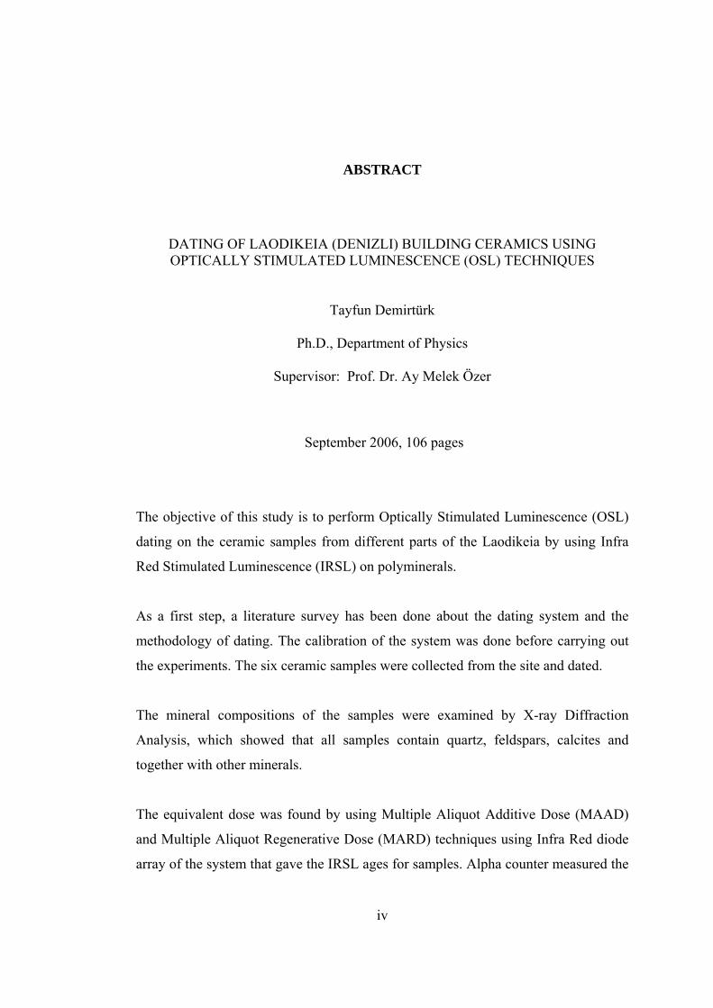
The objective of this study is to perform Optically Stimulated Luminescence (OSL)

dating on the ceramic samples from different parts of the Laodikeia by using Infra

Red Stimulated Luminescence (IRSL) on polyminerals.

As a first step, a literature survey has been done about the dating system and the

methodology of dating. The calibration of the system was done before carrying out

the experiments. The six ceramic samples were collected from the site and dated.

The mineral compositions of the samples were examined by X-ray Diffraction

Analysis, which showed that all samples contain quartz, feldspars, calcites and

together with other minerals.

The equivalent dose was found by using Multiple Aliquot Additive Dose (MAAD)

and Multiple Aliquot Regenerative Dose (MARD) techniques using Infra Red diode

array of the system that gave the IRSL ages for samples. Alpha counter measured the

iv

dose components of uranium and thorium contributions to the annual dose. The

potassium concentration was determined by Atomic Emission Spectrometry. The

cosmic ray component of annual dose was evaluated by the Al2O3:C

Thermoluminescence Dosimeter (TLD) discs which have been placed and kept for 8

and 11 months in the site.

From the data the IRSL ages were calculated for six ceramic samples LDKY-1,

LDKY-2, LDKY-3, LDKY-4, LDKY-5 and LDKY-6 with the help of the OSL

system software. The IRSL ages for these samples, in the given order, are 737 ± 60,

1563 ± 120, 1445 ± 110, 1602 ± 120, 1034 ± 80 and 1034 ± 80 years by using

MAAD technique. The IRSL ages for the same samples are 870 ± 60, 1550 ± 120,

1440 ± 110, 1600 ± 120, 1030 ± 80 and 1030 ± 70 years by using MARD technique.

KEY WORDS: Dating, Optically Stimulated Luminescence (OSL), Infra Red

Stimulated Luminescence (IRSL), Laodikeia, MAAD technique, MARD technique.

v

ÖZ

OPTİK UYARMALI LÜMİNESANS (OSL) TEKNİĞİ İLE LAODIKEIA (DENİZLİ) BİNA SERAMİKLERİNİN TARİHLENDİRİLMESİ

Tayfun Demirtürk

Doktora, Fizik Bölümü

Tez Danışmanı: Prof. Dr. Ay Melek Özer

Eylül 2006, 106 sayfa

Bu çalışmanın amacı Laodikeia kazısının farklı yerlerinden alınan seramik örneklerin

optik uyarmalı lüminesans (OSL) tarihlerinin poliminerallere kızıl ötesi uyarmalı

lüminesans (IRSL) uygulanarak tarihlendirilmesidir.

İlk adım olarak, tarihleme sistemi ve tarihleme metodu hakkında bir literatür

taraması yapıldı. Deneylere başlamadan önce sistemin kalibrasyonu yapıldı. Altı

seramik örnek kazı bölgesinden alındı ve tarihlendi.

Örneklerin mineral içerikleri X-ışını kırınım analizi yöntemiyle belirlendi, temelde

kuvars, feldispat, kalsit ve diğer bazı minerallerin bulunduğu sonucuna varıldı.

Çalışmada eşdeğer doz ölçümü, sistemdeki kızıl ötesi diyotlar dizisi yardımıyla çok

örnekli eklemeli doz (MAAD) ve çok örnekli rejenerasyon doz (MARD)

teknikleriyle yapıldı. Yıllık doza uranyum ve toryum bileşenlerinin katkısı alfa

vi

sayacı ile ölçüldü. Potasyum miktarı atomik emisyon spektrometresi ile bulundu.

Yıllık dozun kozmik ışınlara bağlı bileşeni kazı yerinde toprak altında 8 ve 12 ay

süreyle tutulan Al2O3:C ısı uyarmalı dozimetreleri (TLD) ile belirlendi.

Toplanan veriler ve OSL sisteminin yazılımı ile LDKY-1, LDKY-2, LDKY-3,

LDKY-4, LDKY-5 ve LDKY-6 olarak simgelenen örneklerin MAAD yönteminden

gidilerek IRSL yaşları sırasıyla 737 ± 60, 1563 ± 120, 1445 ± 110, 1602 ± 120, 1034

± 80 ve 1034 ± 80 yıl olarak belirlendi. Aynı örneklerin yaşları MARD yönteminden

gidilerek sırasıyla 870 ± 60, 1550 ± 120, 1440 ± 110, 1600 ± 120, 1030 ± 80 ve

1030 ± 80 yıl olarak bulundu.

Anahtar Sözcükler: Tarihleme, Optik Uyarmalı Luminesans (OSL), Kızılı Ötesi

(Infra Red) Uyarmalı Lüminesans (IRSL), Laodikeia, MAAD tekniği, MARD

tekniği..

vii

TO MY FAMILY

and

TO MY TEACHERS

viii

ACKNOWLEDGEMENTS

I am grateful to my supervisor Prof. Dr. Ay Melek Özer for her guidance and

comprehension.

I would like to thank to Prof.Dr. Şahinde Demirci and Dr. Mustafa Özbakan, for their

special guidance and support throughout my research.

It is a very big pleasure for me to thank to Assoc. Prof. Dr. Enver Bulur and Assoc.

Prof. Dr. H. Yeter Göksu since they shared their endless experiences and knowledge

during my work. If I had never met them, this work was not completed and

meaningful.

I also thank to Prof. Dr. Selahattin Özdemir for his valuable criticisms during the

committee meetings.

I am really thankful to Pamukkale University Excavation Team and especially to

Assoc. Prof. Dr. Celal Şahin and Ali Ceylan who helped me during my visits to the

site of Laodikeia for collecting the ceramic samples, placing and taking back TLDs.

I would like to thank all the people in the physics department for their endless help

during this work.

I also would like to thank to my dear friend and also physics graduate student M.

Altay Atlıhan with whom we spent hours in the dark rooms of OSL laboratories for

preparing the samples and making luminescence measurements.

ix

I am grateful to Prof. Dr. Veysel Kuzucu from Pamukkale University, Physics

Department for guiding and encouraging me to study OSL.

It is also a pleasure for me to thank to Assoc. Prof. Dr. Birol Engin and Hayrünnisa

Demirtaş from Ankara Nükleer Araştırma ve Eğitim Merkezi for their help in TL

measurements of the TLD dosimeters.

I would like to thank to the technician of METU Chemistry Department, Saliha

Pirdoğan for her help during the sample preparations for potassium analysis.

It is a great pleasure for me to thank to my parents, without their valuable support, all

this work was not possible.

Special thanks go to my family who always shared my excitements and enthusiasms

during my study.

x

TABLE OF CONTENTS

PLAGIARISM…………………………………………………………………….. iii

ABSTRACT……………………………………………………………………….. iv

ÖZ………………………………………………………………………………….. vi

DEDICATION……………………………………………………………………... viii

TABLE OF CONTENTS………………………………………………………….. xi

LIST OF TABLES………………………………………………………………… xiv

LIST OF FIGURES……………………………………………………………….. xvi

CHAPTERS

1 INTRODUCTION 1

2 FUNDAMENTALS OF LUMINESCENCE DATING…………………….. 8

2.1 General principles of luminescence dating……………………........ 12

2.2 Mechanism of luminescence……………………………………….. 14

2.3 Signal growth and trap stability…………………………………….. 18

2.4 Anomalous fading………………………………………………….. 22

2.5 Stimulation of the signal……………………………………………. 23

2.6 Materials studied by OSL…………………………………………… 25

3 MATERIALS and METHODS…………………………………………..…. 27

3.1 Samples of Laodikeia Archaeological Site…………………………. 27

3.2 Age Determination………………………………………………….. 30

3.3 Evaluation of Paleodose (Equivalent Dose, Deq)…………………….32

3.3.1 MAAD (Multiple Aliquots Additive Dose) Technique…... 34

3.3.2 MARD (Multiple Aliquots Regenerated Dose) Technique. 35

3.3.3 SAR (Single Aliquot Regeneration) Technique…………...36

3.4 Preheating…………………………………………………………… 37

3.5 Normalization……………………………………………………….. 37

3.6 Sample Preparation…………………………………………………. 38

xi

3.7 Size distribution of the samples…………………………...................39

3.8 Annual Dose Measurements…………………………………………39

3.8.1 Water Saturation and Water Uptake Measurements……... 42

3.8.2 Determination of Potassium in Samples…………………. 43

3.9 Sources of α, β particles and γ rays…………………………………. 45

3.9.1 Contribution of Gamma and Cosmic Rays for Dose Rate... 46

3.10 Supralinearity, Sensitization and Saturation………………………... 46

4 RESULTS and DISCUSSIONS ……………………………………………. 48

4.1 X-Ray Diffraction Analysis (XRD) and Sample Separation……….. 59

4.1.1 Size distribution of the samples 62

4.2 Preheating…………………………………………………………… 64

4.3 Normalization……………………………………………………….. 68

4.4 MAAD (Multiple Aliquots Additive Dose) Technique…………….. 69

4.5 MARD (Multiple Aliquots Regenerated Dose) Technique………….72

4.6 Annual Dose Measurements…………………………………………76

4.6.1 Water Saturation and Water Uptake Measurements……... 76

4.6.2 Alpha Counting for LDKY Samples……………………... 77

4.6.3 Determination of Potassium in Samples…………………. 78

4.6.3.1 Preparation of the samples for potassium

analysis (AES analysis)………………………...80

4.6.4 Contribution of Gamma and Cosmic Rays for Dose Rate.. 81

4.7 Supralinearity, Sensitization and Saturation of the LDKY Samples.. 83

5 CONCLUSION……………………………………………………….......... 85

APPENDICES

A ……………….…...…………………………………………………………. 88

A.1 The Parts of ELSEC 9010 Optical Dating System Comprises………88

A.2 Alpha Counting System…………………………………………….. 92

B ……………….……………………………………………………………….95

B.1 OSL Dating System………………………………………………… 95

B.2 Calibration of Optical Dating System………………………………. 95

B.3 Alpha Counting System…………………………………………….. 100

xii

B.4 Calibration of Alpha Counter……………………………………….. 100

B.5 Dose Rate Calculations of Sr-90 Beta Radiation Source…………… 104

REFERENCES……………………………………………………………………...

xiii

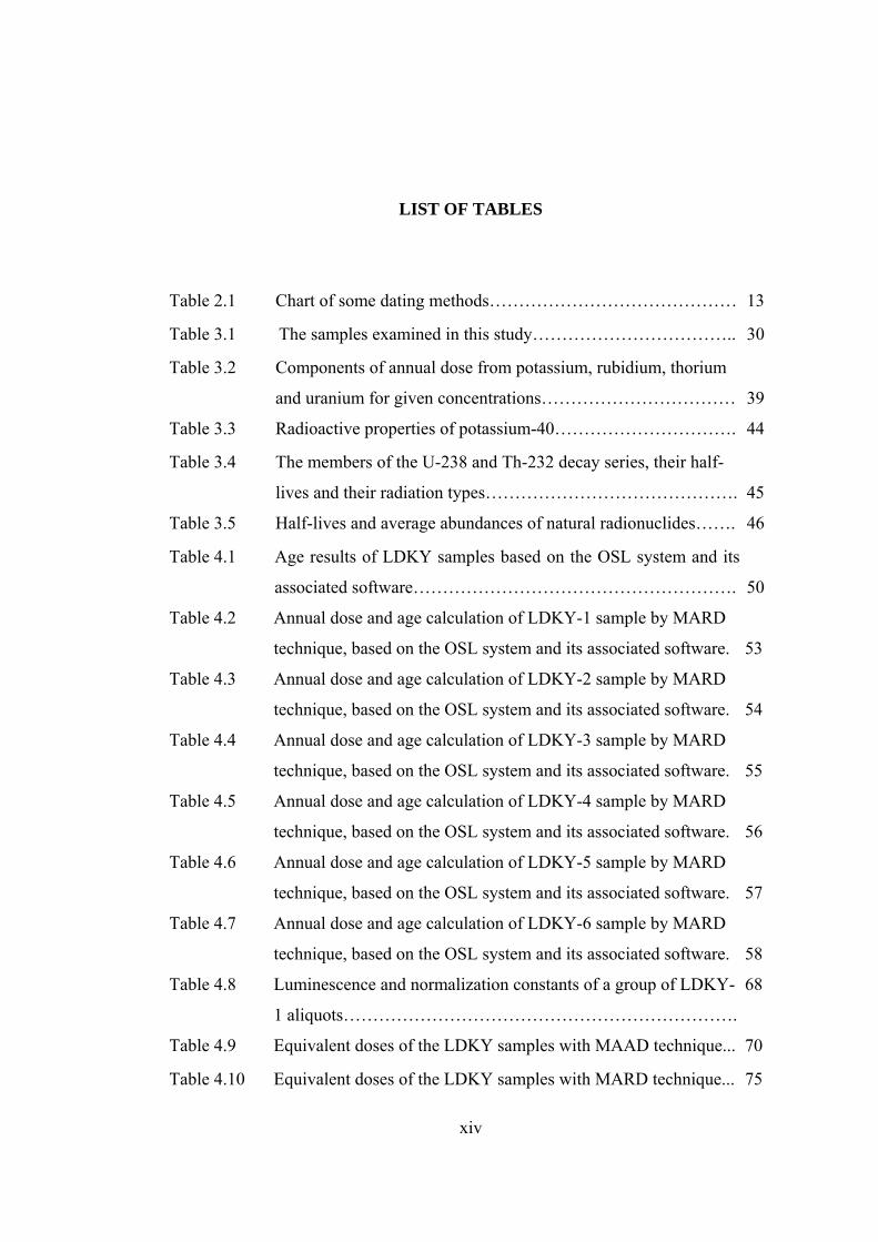
LIST OF TABLES

Table 2.1 Chart of some dating methods…………………………………… 13

Table 3.1 The samples examined in this study…………………………….. 30

Table 3.2 Components of annual dose from potassium, rubidium, thorium

and uranium for given concentrations……………………………

39

Table 3.3 Radioactive properties of potassium-40…………………………. 44

Table 3.4 The members of the U-238 and Th-232 decay series, their half-

lives and their radiation types…………………………………….

45

Table 3.5 Half-lives and average abundances of natural radionuclides……. 46

Table 4.1 Age results of LDKY samples based on the OSL system and its

associated software……………………………………………….

50

Table 4.2 Annual dose and age calculation of LDKY-1 sample by MARD

technique, based on the OSL system and its associated software.

53

Table 4.3 Annual dose and age calculation of LDKY-2 sample by MARD

technique, based on the OSL system and its associated software.

54

Table 4.4 Annual dose and age calculation of LDKY-3 sample by MARD

technique, based on the OSL system and its associated software.

55

Table 4.5 Annual dose and age calculation of LDKY-4 sample by MARD

technique, based on the OSL system and its associated software.

56

Table 4.6 Annual dose and age calculation of LDKY-5 sample by MARD

technique, based on the OSL system and its associated software.

57

Table 4.7 Annual dose and age calculation of LDKY-6 sample by MARD

technique, based on the OSL system and its associated software.

58

Table 4.8 Luminescence and normalization constants of a group of LDKY-

1 aliquots………………………………………………………….

68

Table 4.9 Equivalent doses of the LDKY samples with MAAD technique... 70

Table 4.10 Equivalent doses of the LDKY samples with MARD technique... 75

xiv

Table 4.11 Annual doses of LDKY samples…………………………………. 76

Table 4.12 Water saturation content and water uptake measurements for

LDKY samples……………….......................................................

77

Table 4.13 Unsealed and sealed alpha counts of LDKY samples……………. 78

Table 4.14 Concentrations of potassium standards and their emission

intensity readings by AES………………………………………..

79

Table 4.15 Atomic Emission Spectrometry results of LDKY samples for

potassium content………………………………………………...

80

Table 4.16 Thick Al2O3:C dose response table for gamma irradiation……… 82

Table 4.17 Dose rates of TLD dosimeters for annual γ and cosmic rays of

LDKY samples…………………………………………………...

83

Table B.1 High Tension (HT) voltage calibration data of the PM tube of the

OSL system…………………………………………………..

95

Table B.2 Threshold voltage calibration data of the PM tube of OSL system 96

Table B.3 High Tension (HT) voltage calibration data of the Alpha counter

PM tube…......................................................................................

99

Table B.4 Threshold voltage calibration data of the Alpha Counter PM tube 101

Table B.5 Sr-90 beta radiation source dose rates for feldspar and quartz

components of the sample and its calculated activity values.........

106

xv

LIST OF FIGURES

Figure 1.1 Satellite photo of Laodikeia site………………………………... 4

Figure 1.2 Plan of Laodikeia……………………………………………….. 5

Figure 2.1 Simple types of defects in the lattice structure of an ionic

crystal…………………………………………………………...

10

Figure 2.2 Schematic representation of the event that is being used in the

luminescence dating of pottery and sediments…………………..

14

Figure 2.3 Energy-level representation of the luminescence process……… 15

Figure 2.4 Anomalous fading of the trapped electrons……………………... 22

Figure 3.1 Ceramic Floor tiles of the room which is at the right side of

North of the from church door entrance…………………………

28

Figure 3.2 The ceramic water pipes from the front of the north wall of the

church……………………………………………………………

28

Figure 3.3 The ceramic ceiling tiles from the entrance of the church door… 29

Figure 3.4 Ceramic water pipes and a floor tile from Laodikeia site……… 29

Figure 3.5 The depletion of signal with time……………………………….. 31

Figure 3.6 Block diagram of OSL system and luminescence measurement.. 33

Figure 3.7 Additive dose method of paleodose evaluation…………………. 34

Figure 3.8 Decay curve of luminescence signal from natural or already

dosed sample…………………………………………………….

35

Figure 3.9 Additive regenerated dose method of paleodose evaluation……. 36

Figure 3.10 Luminescence growth characteristic showing supralinear and

sublinear regions.

Figure 4.1 XRD analysis of LDKY-1 ceramic sample……………………... 61

Figure 4.2 TL signal versus temperature curve for the feldspar component

of LDKY-2 sample………………………………………………

65

xvi

Figure 4.3 (a) Luminescence versus temperature graph at constant heating

time. (b) Luminescence versus time graph at 160 oC……………

66

Figure 4.4 Luminescence versus day graph for un-preheated polimineral

aliquots. ………………………………………………………...

67

Figure 4.5 Luminescence counts versus sample # graph…………………… 69

Figure 4.6 Grouping the samples on a tray and adding doses for (MAAD)

luminescence measurements…………………………………….

71

Figure 4.7 Luminescence versus time graph for a polimineral LDKY

sample…………………………………………………………...

71

Figure 4.8 Luminescence versus added Dose graph for LDKY-1 sample..... 72

Figure 4.9 Arrangement of aliquots in the sample tray for natural

luminescence measurements…………………………………….

73

Figure 4.10 Grouping the samples on a tray and adding doses for (MARD)

luminescence measurements…………………………………….

74

Figure 4.11 Luminescence versus added dose graph……………….………... 75

Figure 4.12 Potassium calibration curve…………………………………….. 79

Figure 4.13 Thick Al2O3:C dose response curve for gamma irradiation…….. 82

Figure 4.14 Luminescence versus dose graph for high dose response……… 84

Figure A.1 Sample Tray……………………………………………………. 88

Figure A.2 The graph of fractional transmission versus wavelength of

Schott BG 39 filter………………………………………………

90

Figure A.3 Basic set-up for beta irradiation …………………………….…. 92

Figure A.4 ELSEC 7286 Low Level Alpha Counter system……………….. 93

Figure A.5 Simplified block diagram of alpha counting system…………… 94

Figure B.1 ELSEC 9010 Optical Dating System…………………………… 95

Figure B.2 The apparent intensity versus HT voltage curve.……………….. 97

Figure B.3 The calibration curve of the PM tube, apparent intensity versus

threshold voltage graph………………………………………….

99

Figure B.4 HT voltage calibration curve of the Alpha counter PM tube. ….. 102

Figure B.5 Threshold voltage calibration curve…...………………………... 104

xvii

xviii

CHAPTER 1

INTRODUCTION

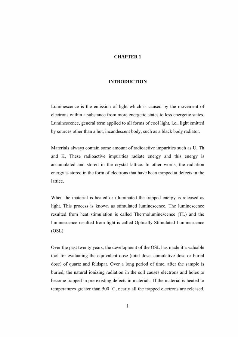
Luminescence is the emission of light which is caused by the movement of

electrons within a substance from more energetic states to less energetic states.

Luminescence, general term applied to all forms of cool light, i.e., light emitted

by sources other than a hot, incandescent body, such as a black body radiator.

Materials always contain some amount of radioactive impurities such as U, Th

and K. These radioactive impurities radiate energy and this energy is

accumulated and stored in the crystal lattice. In other words, the radiation

energy is stored in the form of electrons that have been trapped at defects in the

lattice.

When the material is heated or illuminated the trapped energy is released as

light. This process is known as stimulated luminescence. The luminescence

resulted from heat stimulation is called Thermoluminescence (TL) and the

luminescence resulted from light is called Optically Stimulated Luminescence

(OSL).

Over the past twenty years, the development of the OSL has made it a valuable

tool for evaluating the equivalent dose (total dose, cumulative dose or burial

dose) of quartz and feldspar. Over a long period of time, after the sample is

buried, the natural ionizing radiation in the soil causes electrons and holes to

become trapped in pre-existing defects in materials. If the material is heated to

temperatures greater than 500 oC, nearly all the trapped electrons are released.

1

Also, exposure to sunlight will empty some or all of the traps. These are the

two most common re-setting events. Infrared light has the frequency suitable

for feldspar to stimulate electrons from their traps (Duller, 1991). These

electrons recombine with the trapped holes and produce photons with

frequencies higher than infrared. By measuring the number of emitted photons

resulting from optical stimulation, the age of the sample can be determined.

Huntley et al. (1985) were the first to demonstrate that optically stimulated

luminescence could be used to find the equivalent dose of a sample to the same

level of certainty as previously existing methods such as thermoluminescence

and electron spin resonance.

The procedure for recording Optically Stimulated Luminescence (OSL) during

dating and/or dosimeter applications is to record the luminescence as a function

of illumination time at room temperature (Mckeever et al. 1996). In the

development in OSL instrumentation, two important studies can be mentioned.

One of them is the single grain apparatus described by Duller et al. (1999) and

the linear modulation technique described by Bulur (1996). Initial experiments

with linearly modulated OSL (LM-OSL) were carried out using near-IR

(approximately 880 nm) stimulation on feldspars (Bulur 1996); Bulur and

Göksu (1999).

The first objective of this work is to explain and to apply luminescence

mechanism on nonconductive which is well described in solid state physics.

The second objective is to investigate the potential of applying optically

stimulated luminescence (OSL) for dating studies. The application of OSL

techniques to archaeological ceramics for the past assessment of natural

radiation doses was first suggested by Huntley et al. (1985), and has been

applied in natural dosimeter with great success (Aitken, 1985; Roberts, 1997;

and Wagner, 1998), and the method became firmly established for testing the

authenticity of art ceramics (Stoneham, 1991). These studies have all been

carried out using heated materials. Fortunately, heated materials are frequently

2

available, especially in archeological environments, where heated building

materials such as ceramics are more widely used. Ceramic materials are

suitable in dating, since they mostly have been adequately zeroed in the last

zeroing event (e.g., at the time of manufacture) and they usually have a

sufficient luminescence sensitivity. In this work, experimental studies were

carried out on two ceramic water pipes, two ceramic floor and two ceiling tiles

samples from Laodikeia collected during the 2002 excavation. From now on

the abbreviation LDKY will be used for Laodikeia.

In the Hellenistic era, LDKY was the name given to a number of cities,

founded by the successors of Alexander the Great. Our site is marked by the

river Lykos (Çürüksu), and thus was called LDKY ad Lycum (Roman name,

following earlier Hellenistic practice). LDKY ad Lycum is 6 km north-east of

Denizli, and modern villages incorporated within the Hellenistic city’s borders

are Eskihisar, Goncalı, and Bozburun villages (Figures 1.1 and 1.2). Once

founded by the Seleucid King Antiochos II sometime before B.C. 253, and

named for his wife Laodike, the new city soon became the largest and most

important city in the Lycos Valley. LDKY was completely leveled in the

devastating earthquake in A.D. 494 after which it has never quite recovered.

The site continued to be inhabited, and Byzantine writers occasionally

mentioned Laodikeia, (Şimşek, 2004). Pliny states that the Antiochian city of

LDKY was formerly called Diospolis, “the city of Zeus,” and then Rhoas

(Pliny, AD 77).

For this site no dating study has been done before the LDKY excavation that

has been conducted together with the Archaeology Department of Pamukkale

University (P.U.) and Denizli Museum Directorate teams. However, even

though we are the first sample takers from the site, a M.Sc. thesis has been

done for the LDKY site at P.U. before this study was completed. In the study,

building ceramic samples taken from Laodikeia archaeological site (Denizli)

have been examined.

3

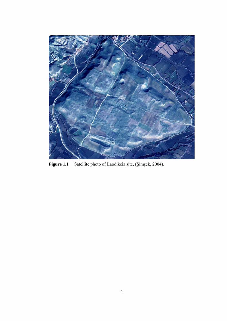
Figure 1.1 Satellite photo of Laodikeia site, (Şimşek, 2004).

4

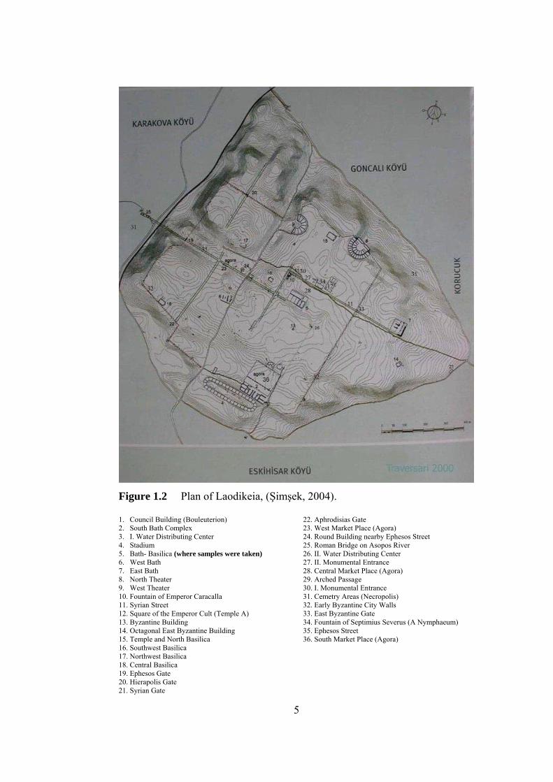
Figure 1.2 Plan of Laodikeia, (Şimşek, 2004). 1. Council Building (Bouleuterion) 2. South Bath Complex 3. I. Water Distributing Center 4. Stadium 5. Bath- Basilica (where samples were taken) 6. West Bath 7. East Bath 8. North Theater 9. West Theater 10. Fountain of Emperor Caracalla 11. Syrian Street 12. Square of the Emperor Cult (Temple A) 13. Byzantine Building 14. Octagonal East Byzantine Building 15. Temple and North Basilica 16. Southwest Basilica 17. Northwest Basilica 18. Central Basilica 19. Ephesos Gate 20. Hierapolis Gate 21. Syrian Gate

22. Aphrodisias Gate 23. West Market Place (Agora) 24. Round Building nearby Ephesos Street 25. Roman Bridge on Asopos River 26. II. Water Distributing Center 27. II. Monumental Entrance 28. Central Market Place (Agora) 29. Arched Passage 30. I. Monumental Entrance 31. Cemetry Areas (Necropolis) 32. Early Byzantine City Walls 33. East Byzantine Gate 34. Fountain of Septimius Severus (A Nymphaeum) 35. Ephesos Street 36. South Market Place (Agora)

5

In Chapter 2, the fundamental concepts of luminescence process are introduced

including the mechanism based on the band model. The chapter discusses the

band model, giving its use to describe the basic concepts of luminescence,

Optically Stimulated Luminescence (OSL) and Thermoluminescence (TL). The

natural materials of OSL, the development of OSL as dating method and the

dosimeter applications are also introduced in this chapter.

Chapter 3 describes the important characteristic features of the OSL system in

the Department of Physics, METU, (the ELSEC 9010 optical dating system).

The samples of OSL are sensitive to light. Therefore, the 9010 system has been

installed in a dark room. The system was established in 1995 and three theses

have been completed in the laboratory already by Yurdatapan, (1997); Buluş-

Kırıkkaya, (2002) and Akoğlu, (2003). The system is equipped with the parts

and software utilized for the OSL studies in this work. There is also an alpha

counter (the ELSEC 7286 low level alpha counter) in the laboratory. In

addition, this chapter introduces the samples used and the experimental

methods including the sample preparation techniques modified during the

work. Two distinct measurements have been carried out in the Laboratory to

determine the age of the LDKY samples. The first measurement is equivalent

dose, the amount of radiation that samples were exposed during burial, which

is measured in grays (Gy). A sample gives off luminescence when exposed to a

light source (Aitken, 1998). Paleodose is determined from the intensity of the

luminescence signal. The second measurement is dose rate, the annual

radiation accumulation rate (Gy/year) of the sample, which is measured from

the concentration of radioactive isotopes within the sample and from

surrounding soil (Aitken, 1985). The dose rate is an approximation of the

radiation a sample has received over time, based on the assumption that the

concentration of radioactive isotopes has remained constant. Fluctuations in the

radiation levels over time are difficult to account for, and result in much of the

uncertainty in OSL ages (Taylor and Aitken, 1997).

6

Chapter 4 tabulates the data and discusses the results of OSL analysis. Age

calculations of LDKY samples carried out with three different processes by

using different radiation coefficients. In addition, this chapter deals with the

results of two quantities which are the equivalent and the annual dose of six

different LDKY ceramic samples. These quantities need to be experimentally

determined to reach an OSL age. An overview is presented of the different

measurement protocols and procedures for equivalent dose (Deq) determination,

with specific attention to those that have been developed for feldspar.

In chapter 5, the conclusions of the studies are given. LDKY has been

destroyed as a result of an earthquake and all the water pipelines have been

renewed as the archaeologists claimed so. The dates of the pipeline samples

may give also the date of the earthquake. Archaeologists also claim that LDKY

has been set into fire during the Seljuk invasion and the dates of the ceiling

tiles may give the date of invasion and fire.

7

CHAPTER 2

FUNDAMENTALS OF LUMINESCENCE DATING

Luminescence is the cool emission of light from material which is caused by

the electrons during their movements from high energy level through low

energy level. It can also be caused by the stimulation of trapped electrons from

metastable energy levels, which are related to their subsequent recombination

under photon-emission.

Electrons trapped at meta-stable sites, become free under certain conditions

such as heating and/or illumination. Some of the electrons reach to the

luminescence centers resulting in emission of light. If the process is done by

heating it is called Thermo Luminescence (TL), if it is done by illumination of

light it is called Optically Stimulated Luminescence (OSL).

Luminescence dating exploits the fact that ionizing radiation from natural

radioactivity and cosmic rays excite electrons, which are partly stored in the

crystal lattice. Since these charges accumulate with time, their amount and thus

the intensity of the luminescence signal can be used for dating (Lang et al.,

1996).

Luminescence dating utilizes sediments, ceramics and stones which contain

quartz and feldspar as natural dosimeters. Quartz and feldspar minerals are

complex solids and present in archaeological and geological samples.

TL or OSL is the luminescence emitted on heating or illumination,

respectively, due to the release of stored energy which has been accumulated in

8

crystalline materials through the action of ionizing radiation from natural

radioactivity. When the material (pottery, brick and so on) is heated, either in

production or during use, and when sediment is exposed to sunlight prior to

deposition, the TL/OSL acquired over geological time is removed. Therefore,

the luminescence "clock" is set to zero. Then, the TL/OSL accumulates in

response to the ionizing radiation received during the burial period of the

material. The time elapsed since last heating or illumination of ancient

materials depends on the total absorbed radiation dose. Knowing the dose

received per year (during burial) the age of the ancient material can be

calculated.

When ionizing radiation (α, β particles and γ rays) interacts with an insulating

crystal lattice, a net redistribution of electronic charge takes place. Electrons

are stripped from the outer shells of atoms and though most return

immediately, a proportion escape and become trapped at ‘meta-stable’ states

within the crystal lattice. The net charge redistribution continues for the

duration of the exposure and the amount of trapped charge is therefore related

to both the duration and intensity of radiation exposure.

The effect of radiation such as gamma rays, beta particles (electrons), and

alpha particles on a sample can be expressed in terms of a quantity known as

absorbed dose. This is a measure of the radiation dose (as energy per unit

mass) absorbed by a specific sample. Its SI unit is the Gray (Gy). An older unit,

the rad (from radiation absorbed dose) is still in common use. The two units

are related as follow:

1 Gy = 1 J/kg = 100 rad

Dating of archaeological materials by the OSL method depends on the fact

that, when mineral grains are isolated from daylight by burial, they begin to

accumulate electrons in their traps. These electrons result from exposure to the

9

ionizing radiation emitted by the decay of naturally occurring radioisotopes,

K-40, Th-232 and U-238, within the material. If the flux of ionizing radiation is

constant, then the burial time of the grains can simply be determined by

dividing the total dose (also called as burial dose, equivalent dose or

paleodose) which have been accumulated during burial time to the Dose-Rate

i.e.,

(Gy/year) Rate-Dose(Gy) Dose Burial )year( Time Burial = (2.1)

The dose-rate is also called as annual dose and it is equal to the dose received

per year.

The dose rate (annual dose) represents the yearly rate at which energy is

absorbed from the flux of nuclear radiation provided by thorium, uranium and

potassium-40 in the material, as well as by cosmic rays. The annual dose is

assumed to be constant and evaluated by the assessment of the radioactivity of

the material determined both in the laboratory and on-site by using dosimeters.

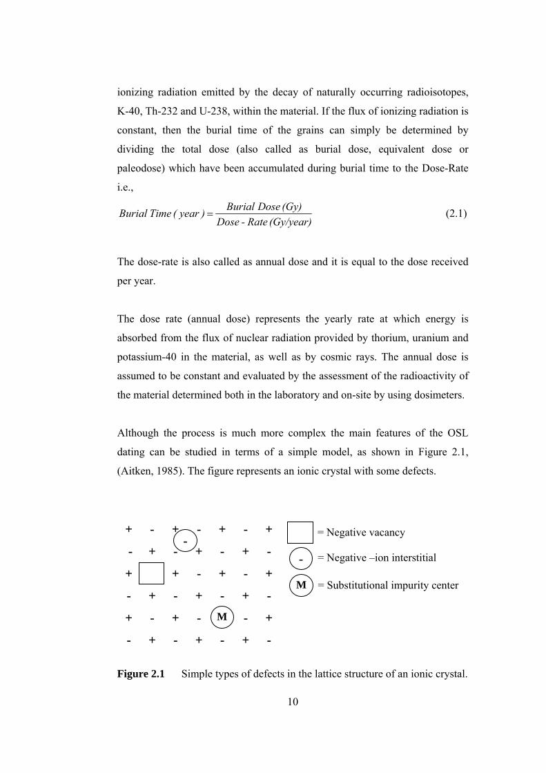
Although the process is much more complex the main features of the OSL

dating can be studied in terms of a simple model, as shown in Figure 2.1,

(Aitken, 1985). The figure represents an ionic crystal with some defects.

+ - + - + - +

- + - + - + -

+ + - + - +

- + - + - + -

+ - + - - +

- + - + - + -

M

- -

M

= Negative vacancy

= Negative –ion interstitial

= Substitutional impurity center

Figure 2.1 Simple types of defects in the lattice structure of an ionic crystal.

10

The defects in the mineral crystals i.e, negative ion vacancy, and negative ion

interstitial, and substitıtional impurity centers behave as the trap for electrons.

The ionizing radiation from the decay of the naturally occurring radioisotopes

(e.g. U, Th, K) interacts with a crystalline substance, freeing electrons from

their normal atomic sites. Some of these electrons become trapped at the defect

centers and, if the trap depth (E) is large enough, they will remain there

indefinitely on a geological time scale. The number of these electrons is thus a

measure of the total radiation dose since some event in which all the traps were

emptied. It is assumed that electrons caught in traps stay in there indefinitely.

In fact, the lifetime of an electron in a trap is not infinite but has a value that

depends on the type of the trap (Aitken, 1989).

Luminescence dating is particularly appropriate when radiocarbon dating is not

possible (either where no suitable material is available or for ages beyond the

radiocarbon age limit). When the relationship between the organic materials

and the archaeological context is uncertain, the particular advantage of

luminescence dating is that the method provides a date for the archaeological

artifact or deposit itself, rather than for organic material in assumed

association. In the case of OSL dating, suitable material is usually available all

throughout the site.

The age range for pottery and other ceramics covers the entire period in which

these materials have been produced. The typical range for burnt flint, stone or

sediment (burnt or un-burnt) is from about 50 to 300,000 years. The error

limits on the dates obtained are typically in the range ±3 to ±8%, although

recent technical developments now allow luminescence measurements to be

made with a precision of in favorable circumstances.

Ceramics and burnt flint or stone must have been heated to at least up to 350°C

in antiquity. The samples must be large enough to ensure that sufficient sample

is available for dating after the removal of the outer 2 mm layer over the entire

11

surface. This removal will depend on the composition of the material.

Typically a fragment whose volume is equivalent to at least 1 cm x 2cm x 2cm

is required for measurement. In addition, as an absolute minimum, it is

necessary to provide at least 100 gram soil or sediment sample in which the

pottery, flint or other material was buried

It is preferred for the person that does luminescence dating should visit the site

(during the excavation in archaeological contexts) either to collect samples or

at least to advise for sample collection, and to measure the environmental

contribution to the annual radiation dose using a portable gamma spectrometer

or dosimeter. This can significantly improve the dating precision.

It is highly desirable that the deposits are as uniform as possible and that

pottery or flint are not collected from near boundaries (edges of a trench or

changes in soil type), or from a depth less than 30 cm from the present ground

surface (Aitken, 1985).

2.1 General principles of luminescence dating

The luminescence dating is one of the radioactive dating techniques and it

belongs to the subgroup which is based on the accumulation of radiation

damage in a mineral. The radiation damage accumulation is the result of

exposure to a low-level ionizing radiation in the soil. The longer the exposition

of a mineral to the ionizing natural radiation the greater the intensity of the

radiation accumulation is. The intensity of the radiation accumulation is

consequently a measure for the total dose (the total amount of energy absorbed

from the ionizing radiation) of the mineral that has received over a certain

period of time.

In luminescence dating, the density of the radiation accumulation is detected as

a small amount of light, which is called luminescence. The radiation

12

accumulation which is the hidden luminescence signal can be removed or set to

zero by exposing to heat or light. For ancient pottery the ‘zeroing’ took place

during manufacturing, when it was baked in a kiln. In the context of sediment

dating, the zeroing event was the exposing to daylight during erosion, transport

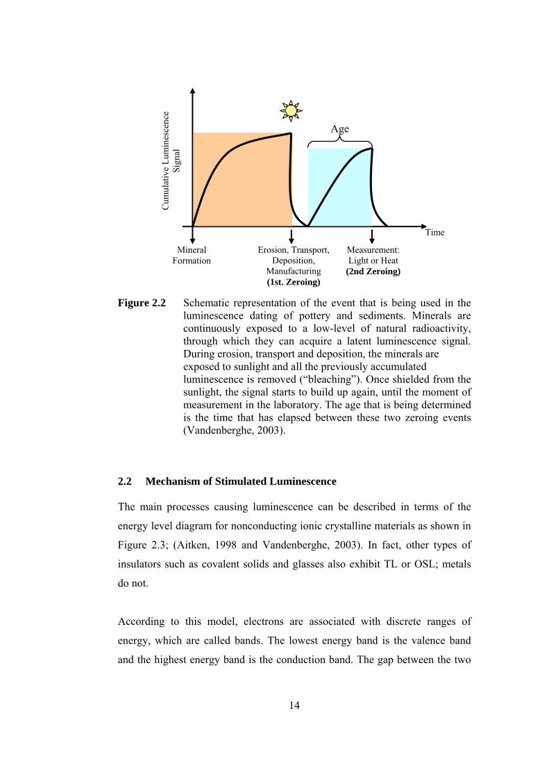
and deposition of the mineral grains (Figure 2.2) (Vandenberghe, 2003). This

zeroing through exposure to sunlight is also called bleaching. Once the zeroing

agent is no longer active, the luminescence signal can start to build up again.

For instance, in the case of sedimentary mineral grains, the clock starts ticking

when the samples were shielded from the sunlight by burial under other grains

deposited on top of them. A comparison of the luminescence dating with the

other dating methods is given in Table 2.1.

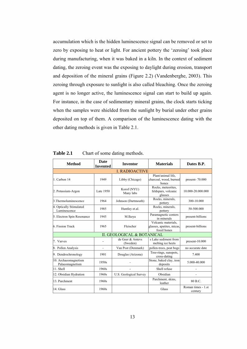
Table 2.1 Chart of some dating methods.

Method Date Invented Inventor Materials Dates B.P.

I. RADIOACTIVE

1. Carbon 14 1949 Libby (Chicago) Plant/animal life,

charcoal, wood, burned bones

present- 70.000

2. Potassium-Argon Late 1950 Korof (NYU) Many labs

Rocks, meteorites, feldspars, volcanic

glasses 10.000-20.000.000

3.Thermoluminescence 1964 Johnson (Dartmouth) Rocks, minerals, pottery 300-10.000

4. Optically Stimulated Luminescence 1985 Huntley et.al. Rocks, minerals,

pottery 50-500.000

5. Electron Spin Resonance 1945 M.Ikeya Paramagnetic centers in minerals present-billions

6. Fission Track 1965 Fleischer Volcanic materials,

glasses, apatites, micas, fossil bones

present-billions

II. GEOLOGICAL & BOTANICAL 7. Varves - de Geer & Antevs

(Sweden) s Lake sediment from

melting ice heets present-10.000

8. Pollen Analysis - Van Post (Denmark) pollen-trees, peat bogs no accurate date

9. Dendrochronology 1901 Douglas (Arizona) Tree-rings, sunspots, cross-dating 7.400

10. Archaeomagnetism Palaeomagnetism 1950s - Stone, baked clay, iron

deposits 5.000-40.000

11. Shell 1960s - Shell refuse -

12. Obsidian Hydration 1960s U.S. Geological Survey Obsidian -

13. Parchment 1960s Parchment, skins, leather 80 B.C.

14. Glass 1960s Glass Roman times - 1.st century

13

Age

Cum

ulat

ive

Lum

ines

cenc

e Si

gnal

Mineral Formation

Erosion, Transport, Deposition,

Manufacturing (1st. Zeroing)

Measurement: Light or Heat

(2nd Zeroing)

Tim

e

Figure 2.2 Schematic representation of the event that is being used in the luminescence dating of pottery and sediments. Minerals are continuously exposed to a low-level of natural radioactivity, through which they can acquire a latent luminescence signal. During erosion, transport and deposition, the minerals are exposed to sunlight and all the previously accumulated luminescence is removed (“bleaching”). Once shielded from the sunlight, the signal starts to build up again, until the moment of measurement in the laboratory. The age that is being determined is the time that has elapsed between these two zeroing events (Vandenberghe, 2003).

2.2 Mechanism of Stimulated Luminescence

The main processes causing luminescence can be described in terms of the

energy level diagram for nonconducting ionic crystalline materials as shown in

Figure 2.3; (Aitken, 1998 and Vandenberghe, 2003). In fact, other types of

insulators such as covalent solids and glasses also exhibit TL or OSL; metals

do not.

According to this model, electrons are associated with discrete ranges of

energy, which are called bands. The lowest energy band is the valence band

and the highest energy band is the conduction band. The gap between the two

14

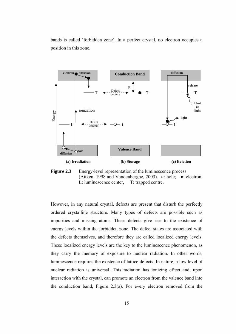
bands is called ‘forbidden zone’. In a perfect crystal, no electron occupies a

position in this zone.

L

Defect centers T

E

Conduction Band

Valence Band diffusion

hole

diffusion electron

L

T

Defect centers L

T

ionization

diffusion

release

Heaor

light

light

t

(a) Irradiation (c) Eviction (b) Storage

Ener

gy

Figure 2.3 Energy-level representation of the luminescence process (Aitken, 1998 and Vandenberghe, 2003). ○: hole; ●: electron, L: luminescence center, T: trapped centre.

However, in any natural crystal, defects are present that disturb the perfectly

ordered crystalline structure. Many types of defects are possible such as

impurities and missing atoms. These defects give rise to the existence of

energy levels within the forbidden zone. The defect states are associated with

the defects themselves, and therefore they are called localized energy levels.

These localized energy levels are the key to the luminescence phenomenon, as

they carry the memory of exposure to nuclear radiation. In other words,

luminescence requires the existence of lattice defects. In nature, a low level of

nuclear radiation is universal. This radiation has ionizing effect and, upon

interaction with the crystal, can promote an electron from the valence band into

the conduction band, Figure 2.3(a). For every electron removed from the

15

valence band is an electron vacancy, termed a hole, is left behind and both the

electron and hole are free to move throughout the crystal. In this way, energy

of the nuclear radiation is taken up. The energy can be released again (usually

as heat) by recombination. Although most of the charges recombine directly,

another possibility is that the electron and the hole are trapped at the defect

centers traps. In this case, the radiation energy is stored temporarily in the

crystal lattice and the system is said to be in a metastable state, Figure 2.3(b).

Energy is required to remove the electrons out of the traps and to return the

system to a stable situation. The amount of energy that is necessary is

determined by the depth (E) of the trap below the conduction band. This trap

depth is one of the parameter to determine the life time of an electron in the

trap. To empty deeper traps, more energy will be required and those traps are

more stable over time. For dating, we are only concerned in those traps deep

enough (i.e. ~1.6 eV or more) for the age of at least several million years. By

heating or shinning a light on the samples, electrons are removed from the

electron traps and some of these reach luminescence centers (L) resulting in

emission of light (Figure 2.3(c)). As mentioned before, if the process is done

by heating it is called TL, if shining of light is used it is called OSL.

In summary, the steps were given in Figure 2.3 are as follows,

1. Ionization of electrons by nuclear radiation.

2. Immediate capture of some of these electrons at traps, where they

remain stored as long as the temperature is not raised or not exposed to

light.

3. Eviction from the traps due to heating or exposing to light during the

measurement process centuries later.

16

4. Recombination almost instantaneously, some of these evicted electrons

with luminescence centers, accompanied by emission of light. The

amount of light is proportional to the number of trapped electrons,

which in turn is proportional to the amount of nuclear radiation to

which the crystal has been exposed and therefore to the time that has

elapsed since the traps were last emptied.

The main difference between TL and OSL is the stimulating source. Although

the mechanisms are the same for both techniques there are some advantages of

OSL over TL. These can be summarized as follows:

• OSL can be measured near or at room temperature hence it is less

destructive and more sensitive method than TL.

• Parts of OSL signal can be measured many times on same sample

however in TL this is impossible since the measurement involves the

total erasure of the signal. Therefore, for normalization of aliquots

short shines of OSL can be used.

• After measurement of OSL a TL signal can be measured on the same

sample however the reverse may not be possible.

• OSL measures the electrons held in traps, which are the most sensitive

to light and is thus particularly important in dating geological sediment

samples, which had been zeroed in the past by sun bleaching.

Furthermore, in many cases, OSL has the same dose response as TL.

(Bøtter -Jensen, 2000).

There are some studies for more complex and detailed accounts on the physical

theory of the process (McKeever, 1985; Chen and McKeever, 1997; and Bøtter

Jensen et al., 2003a).

17

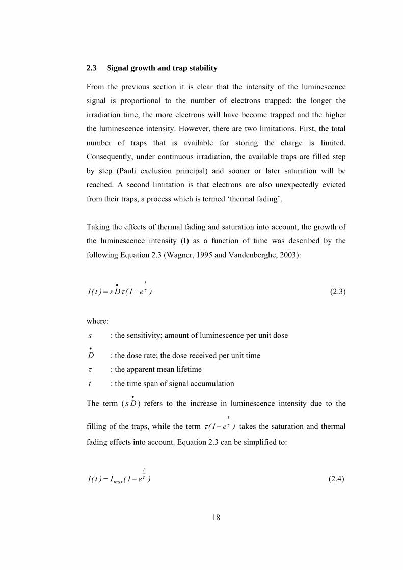
2.3 Signal growth and trap stability

From the previous section it is clear that the intensity of the luminescence

signal is proportional to the number of electrons trapped: the longer the

irradiation time, the more electrons will have become trapped and the higher

the luminescence intensity. However, there are two limitations. First, the total

number of traps that is available for storing the charge is limited.

Consequently, under continuous irradiation, the available traps are filled step

by step (Pauli exclusion principal) and sooner or later saturation will be

reached. A second limitation is that electrons are also unexpectedly evicted

from their traps, a process which is termed ‘thermal fading’.

Taking the effects of thermal fading and saturation into account, the growth of

the luminescence intensity (I) as a function of time was described by the

following Equation 2.3 (Wagner, 1995 and Vandenberghe, 2003):

)e1(Ds)t(Itττ −=

• (2.3)

where:

s : the sensitivity; amount of luminescence per unit dose •D : the dose rate; the dose received per unit time

τ : the apparent mean lifetime

t : the time span of signal accumulation

The term ( ) refers to the increase in luminescence intensity due to the

filling of the traps, while the term

•Ds

)e1(tττ − takes the saturation and thermal

fading effects into account. Equation 2.3 can be simplified to:

)e1(I)t(It

maxτ−= (2.4)

18

where, “ ”, i.e. the maximum intensity that can be built up and

measured. The apparent mean lifetime, τ, can be written as follow (Wagner,

1995; Vancraeynest, 1998; Vandenberghe, 2003):

τ•

= DsImax

Ts

Ts

τττττ+

= (2.5)

where, τs is a decay constant (also saturation characteristic) taking into account

that the number of traps is limited and τT is the mean lifetime. The mean

lifetime is the average residence time of electrons in a given type of trap and at

a certain given temperature T.

It is clear from the above Equation 2.5 that both the saturation characteristic

(τs) and the long-term stability of the signal (τT) determine the highest intensity

to which a luminescence signal can grow, and hence also the upper dating limit

that can be attained.

Under these considerations the saturation dose of the mineral depends on the

first approximation (saturation). For instance, quartz generally saturates at a

much lower dose compared to feldspars. Prescott and Robertson (1997)

proposed an age limit of 100-200 ka (1ka = 103 year) for quartz while age

provides up to 1 Ma (1Ma = 106 year) for feldspar, if they do not suffer from

anomalous fading (see section 2.4). However, if the quartz mineral is exposed

to a very low-level of natural radioactivity, the traps are also less rapidly filled,

which extends the age range over which this mineral can be used. When a low

dose rate enabled, quartz-based luminescence ages was obtained as old as

~700-800 ka (Huntley et al., 1993, 1994; Huntley and Prescott, 2001).

Besides the limitations imposed by signal saturation, the mean lifetime also

restricts the age range over which a luminescence signal can be used for dating;

the luminescence signal employed should be sufficiently stable. This means

19

that only those traps should be evicted during the measurement from which

there has been a negligible loss of electrons over the time span that is being

dated. It is usually assumed that unstable luminescence arises from shallow

traps while stable luminescence arises from deep traps. The probability for

electrons to escape from a deep trap is low, and the lifetime (τT) is

correspondingly high. The possibility exists due to the random chance of an

abnormally large energetic lattice vibration which causes the eviction.

At a constant temperature, the number of trapped electrons, n, decays

exponentially with time according to Equation 2.6:

T

12 tt

12 e)t(n)t(n τ−

−= (2.6)

In the context of dating, the time interval t2-t1 of interest is the age of the

sample. However, when calculating the fraction of electrons that spontaneously

escape during this period of time, it must be taken into account that there are no

electrons in their traps at time zero [i.e. at t1 = 0, n(t1) = 0] and that they

become trapped at a uniform rate thereafter. For such a situation, it can be

shown to a good approximation (Aitken, 1985) that the fractional loss of

luminescence due to escape during the age span of the sample, ts (= t2-t1), is

given by ½(ts/τT) as long as ts does not exceed one third of τΤ. This means that

to avoid an age underestimation by e.g. 5%, the lifetime consequently needs to

be at least 10 times the age.

The trapped electron mean lifetime, in the case of first order kinetics, is given

by the following equation (Aitken, 1985; Vandenberghe, 2003)

T.kE

1T es−=τ (2.7)

where:

s : the frequency or pre-exponential factor (in s-1); this may be thought of

as the number of attempts to escape per second

20

E : the depth of the trap (in eV)

T : the absolute temperature (in K)

k : Boltzmann’s constant (8.6173×10-5 eV K-1)

Predicting lifetimes (τT) is useful as it helps to establish the likely time-range

over which a given signal from a given mineral will be used. It is also

important because a measured OSL signal does not contain any intrinsic

information with regard to its stability. Some further considerations regarding

signal stability and lifetimes that are directly relevant to the present work are

discussed in Chapter 4.The OSL signal arises from electrons that are evicted

out of all traps that are sensitive to the light employed for stimulation, whether

these traps are deep (stable) or shallow (unstable).

In nature, the filling rate of the traps is low. The luminescence signal measured

from a natural sample will be primarily associated with deep traps since the

shallow traps loose their electrons quickly due to thermal fading. However, it is

necessary to irradiate the sample in the laboratory, and to compare the artificial

luminescence signals so induced with the natural signal. In the laboratory, the

doses are added to the samples at a much higher rate than those in nature. Now,

the shallow traps will be filled and, owing to the short time scale over which

the experiments are carried out, they may contribute significantly to the

artificial signal. Therefore, it is necessary to remove this unstable

“contaminating” luminescence by emptying the shallow traps before the signal

is measured. This emptying is usually accomplished by heating the sample

prior to measurement. This treatment is called preheating and it will be further

discussed in Chapter 3 and 4, together with the additional reasons for why it is

necessary.

21

2.4 Anomalous fading

Equation 2.7 describes the expected mean lifetime of an electron in a trap of

depth E and escape frequency s at a storage temperature T. For deep traps and

at low temperatures, the lifetime will consequently be quite large and leakage

of electrons from these traps will be low. However, it has been observed for

many materials that the electrons are released from their traps at a much faster

rate than those predicted by Equation 2.7. This fading of the luminescence

signal is therefore termed ‘anomalous’ (abnormal) fading, (Figure 2.4). For

natural minerals relevant to dating, the result of anomalous fading is an age

shortfall, regardless of whether TL or OSL signals are being used. The effect

was first observed by Wintle et al. (1971) and Wintle (1973), when trying to

date feldspars extracted from volcanic lava with TL. The ages obtained were

significantly lower than the expected ages for the lava flows. The effect has

been subsequently observed and investigated in a number of studies (Wintle,

1977; Clark and Templer, 1988; Spooner, 1992; 1994; Visocekas, 2000;

Auclair et al., 2003).

Conduction Band

Trap depth

b

c

a

d

Trap

Recombination Center

Figure 2.4 Anomalous fading of the trapped electrons. Escape roots from a trap: a) thermal tunneling, b) thermally or optically assisted tunneling, c) and d) thermal or optical eviction (Visocekas et al., 1976 and Aitken, 1985).

22

A number of natural dosimeters, most notably zircon and several types of

mong all of the mechanisms that have been proposed to explain anomalous

.5 Stimulation of the signal

clear that the same production mechanism is

OSL, the electron escapes from its trap as the result of the absorption of a

feldspars suffer from anomalous fading. It is generally accepted, however, that

quartz is not affected by this phenomenon. Wintle (1973) reported no loss in

TL after storage of the quartz for two years, while Roberts et al. (1994) did not

detect any loss in the OSL from quartz after seventy days storage at room

temperature. Readhead (1988) found anomalous fading of TL in quartz from

Southeastern Australia, but Fragoulis and Stoebe (1990) and Fragoulis and

Readhead (1991) subsequently found fading feldspar inclusions to be present in

these quartz grains.

A

fading, quantum mechanical tunneling of electrons to nearby recombination

centers is probably the most accepted one. For more details on this, and other

suggested explanations, reference is made to Aitken (1985), Aitken (1998),

McKeever (1985), Chen and McKeever (1997) and Bøtter-Jensen et al.

(2003a). These publications also provide a comprehensive overview on the

reported observations of the effect, and address practical issues that are

relevant in a dating context, such as ways to detect, overcome or correct for

anomalous fading. Recent work on the correction for fading in feldspar

minerals is that by Auclair et al. (2003) and Lamothe et al. (2003).

2

From sections 2.1 and 2.2, it is

responsible for the two luminescence phenomena, TL and OSL, and that the

only difference between them lays in the way the electrons are stimulated out

of their traps.

In

photon of light with a sufficient energy. The rate of eviction depends on the

intensity of the stimulating light, the wavelength of the light and the sensitivity

23

of the trap to light. There is also a dependency on the temperature of the

material.

The intensity refers to the number of photons arriving at within a certain time.

It can easily be understood that the more photons arrive at per unit of time, the

more electrons will be stimulated out of their traps. The light-sensitivity of a

trap is not well described by the trap depth E; it depends on other

characteristics of the trap, as well as on the wavelength of the stimulating light

(Aitken, 1998). In general, shorter wavelengths (higher energy) are more

effective in stimulating electrons from their traps. The trap depth is given as,

E)nm(

)eV(λ1240

= (2.8)

ence, a first expectation would be that in order to evict an electron from a trap H

having sufficient depth, say 1.4 eV, to retain electrons without leakage on a

long term time scale the wavelength of the stimulating light needs to be shorter

than ⎟⎠⎞

⎜⎛ = nm 8861240 . This means that eviction can be possible even with a

stimulation and luminescence emission wavelength regions need to be well

separated from each other. Furthermore, the wavelength of the luminescence

signal that is used for dating should be shorter than the one used for

stimulation. The type of mineral that is under investigation also plays a role in

the selection of the most appropriate light source for stimulation. A given

wavelength can be effective for stimulating a luminescence signal from some

minerals, whereas for other minerals, it proves to be not suitable.

⎝ 4.1

wavelength as long as that of the near-infrared (700-800 nm). Consequently,

rom the above considerations, it was found that for quartz, for instance, F

stimulation by visible light with a wavelength somewhere in the blue to green

region of the spectrum is appropriate. For feldspathic minerals, on the other

hand, it has been found that long wavelengths, in the infrared region (800-900

24

nm), can also be used (Hütt et al., 1988). It can be mentioned here that longer

wavelengths can also be effective, if the temperature of the sample is raised.

This effect is called thermal assistance.

Depending on the wavelength used for stimulation, the resulting luminescence

is termed infrared stimulated luminescence (IRSL), blue-plus-green stimulated

luminescence (BGSL), green light stimulated luminescence (GLSL or GSL) or

blue light stimulated luminescence (BLSL or BSL). OSL generally refers to

any luminescence signal that is obtained via stimulation with light, regardless

of the wavelength. In some literature, however, the term OSL should be read as

encompassing visible stimulation wavelengths only. To avoid confusion, it is

therefore more appropriate to specify the stimulation wavelength, for example

as OSL (514.5 nm).

2.6 Materials Studied by OSL

rtz are the most widely used minerals in the

or coarse (sand-sized) grains (of ~0.1 mm in diameter), the different mineral

esides feldspar and quartz, ZrSiO4 (Zircon) (Smith et al., 1986; Smith, 1988)

and Ca5(PO4)3(F,OH,Cl) (Apatite) (Smith et al., 1986) have been found to emit

OSL as well.

Minerals such as feldspars and qua

optical dating. The choice of the mineral that is being used usually depends on

the availability of the mineral within the sample, the age of the samples and so

on. Quartz saturates at lower doses than feldspars, and so the use of feldspar

might prove to be advantageous for dating older deposits.

F

fractions can be easily separated from each other, this is not the case for fine

(silt-sized) grains (of ~0.01 mm in diameter). Usually, the measurements are

then carried out on the polymineral fine fraction, which is a mixture of all

kinds of minerals with a grain size within the range 4-11 μm.

B

25

Compared to feldspar and quartz, these minerals occur in materials in much

smaller quantities, which limit their use in any case. Finally, it is perhaps worth

mentioning that also glass extracted from volcanic ash deposits has been found

to emit OSL (Berger and Huntley, 1994; Berger and Neil, 1999). Encouraging

initial results were obtained, but further work is necessary to establish the full

extent to which the glass might be suitable for optical dating.

26

CHAPTER 3

MATERIALS and METHODS

In this chapter, sampling, the OSL dating and Alpha counting systems, dose

rate calculations of Sr-90 β radiation source, sample preparation techniques,

measurement techniques of equivalent dose and annual dose of samples are

described. In order to reduce noise level of the measurements, OSL dating and

Alpha counting systems were explained and calibrated as given in Appendix A

and B.

3.1 Samples of Laodikeia Archaeological Site

The ceramic samples of Laodikeia were taken under the red light during the

night excavation. Before and while taking the samples, opinions and ideas of

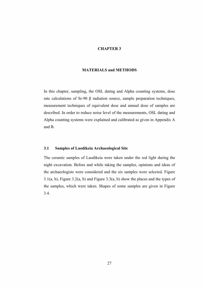
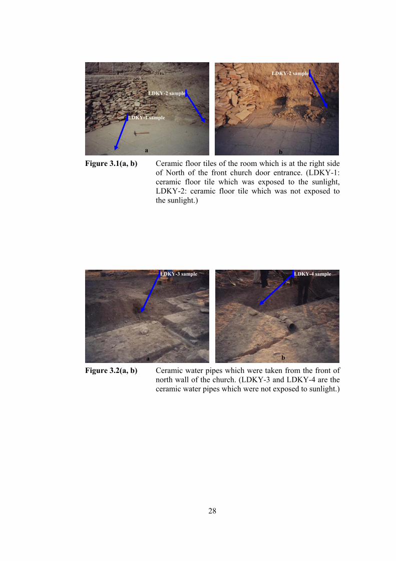
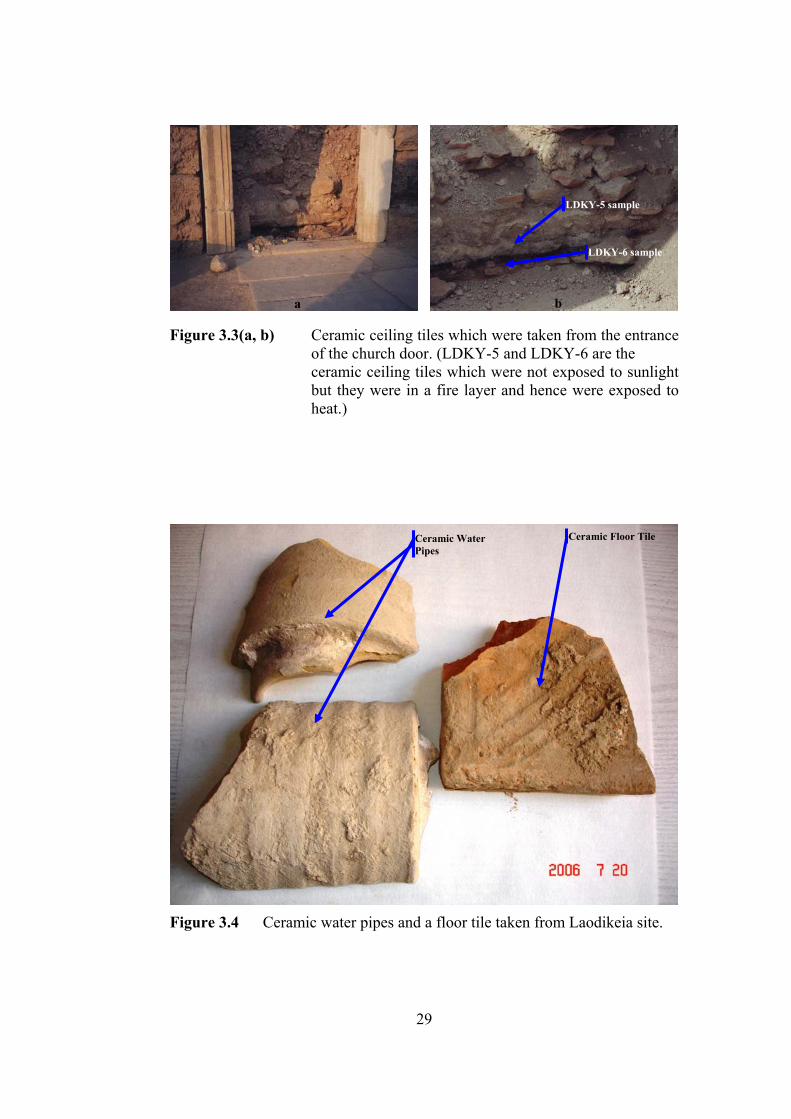
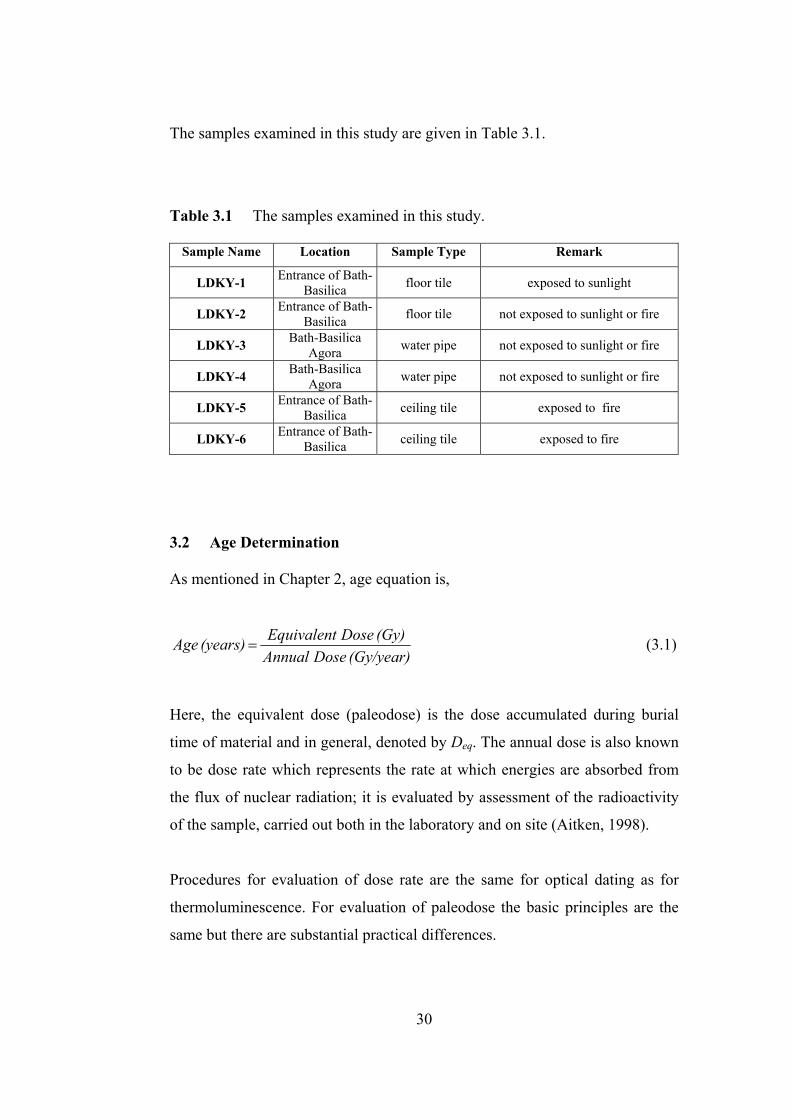
the archaeologists were considered and the six samples were selected. Figure

3.1(a, b), Figure 3.2(a, b) and Figure 3.3(a, b) show the places and the types of

the samples, which were taken. Shapes of some samples are given in Figure

3.4.

27

LDKY-2 sample

LDKY-1 sample

LDKY-2 sample

a b

Figure 3.1(a, b) Ceramic floor tiles of the room which is at the right side of North of the front church door entrance. (LDKY-1: ceramic floor tile which was exposed to the sunlight, LDKY-2: ceramic floor tile which was not exposed to the sunlight.)

LDKY-3 sample LDKY-4 sample

a b

Figure 3.2(a, b) Ceramic water pipes which were taken from the front of north wall of the church. (LDKY-3 and LDKY-4 are the ceramic water pipes which were not exposed to sunlight.)

28

LDKY-5 sample

LDKY-6 sample

a b

Figure 3.3(a, b) Ceramic ceiling tiles which were taken from the entrance of the church door. (LDKY-5 and LDKY-6 are the ceramic ceiling tiles which were not exposed to sunlight but they were in a fire layer and hence were exposed to heat.)

Ceramic Floor TileCeramic Water Pipes

Figure 3.4 Ceramic water pipes and a floor tile taken from Laodikeia site.

29

The samples examined in this study are given in Table 3.1.

Table 3.1 The samples examined in this study.

Sample Name Location Sample Type Remark

LDKY-1 Entrance of Bath-Basilica floor tile exposed to sunlight

LDKY-2 Entrance of Bath-Basilica floor tile not exposed to sunlight or fire

LDKY-3 Bath-Basilica Agora water pipe not exposed to sunlight or fire

LDKY-4 Bath-Basilica Agora water pipe not exposed to sunlight or fire

LDKY-5 Entrance of Bath-Basilica ceiling tile exposed to fire

LDKY-6 Entrance of Bath-Basilica ceiling tile exposed to fire

3.2 Age Determination

As mentioned in Chapter 2, age equation is,

(Gy/year) Dose Annual(Gy) Dose Equivalent (years) Age = (3.1)

Here, the equivalent dose (paleodose) is the dose accumulated during burial

time of material and in general, denoted by Deq. The annual dose is also known

to be dose rate which represents the rate at which energies are absorbed from

the flux of nuclear radiation; it is evaluated by assessment of the radioactivity

of the sample, carried out both in the laboratory and on site (Aitken, 1998).

Procedures for evaluation of dose rate are the same for optical dating as for

thermoluminescence. For evaluation of paleodose the basic principles are the

same but there are substantial practical differences.

30

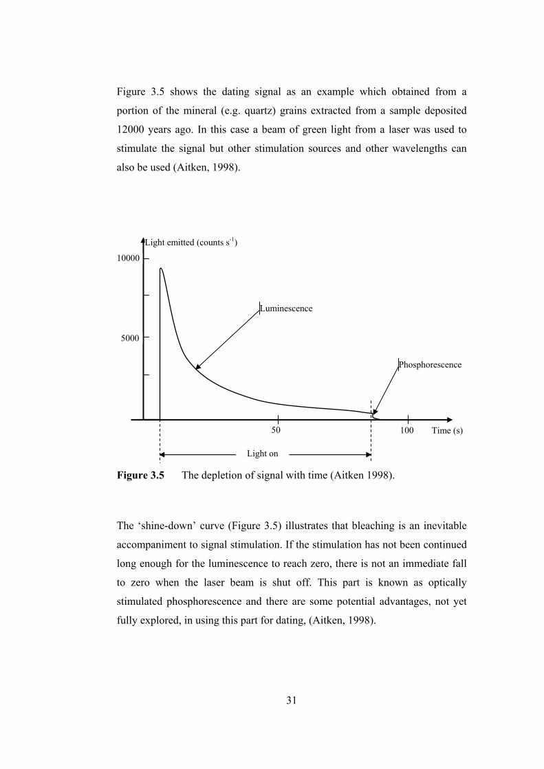
Figure 3.5 shows the dating signal as an example which obtained from a

portion of the mineral (e.g. quartz) grains extracted from a sample deposited

12000 years ago. In this case a beam of green light from a laser was used to

stimulate the signal but other stimulation sources and other wavelengths can

also be used (Aitken, 1998).

Luminescence

Phosphorescence

Light on

Light emitted (counts s-1)

5000

Time (s)100 50

10000

Figure 3.5 The depletion of signal with time (Aitken 1998).

The ‘shine-down’ curve (Figure 3.5) illustrates that bleaching is an inevitable

accompaniment to signal stimulation. If the stimulation has not been continued

long enough for the luminescence to reach zero, there is not an immediate fall

to zero when the laser beam is shut off. This part is known as optically

stimulated phosphorescence and there are some potential advantages, not yet

fully explored, in using this part for dating, (Aitken, 1998).

31

3.3 Evaluation of Paleodose (Equivalent Dose, Deq)

One of the most important steps in determining the age of the sample is to

measure the equivalent dose (paleodose). There are various methods for

measuring the paleodose such as Multiple Aliquots Additive Dose (MAAD),

Multiple Aliquots Regeneration Dose (MARD) and Single Aliquots

Regeneration (SAR) techniques.

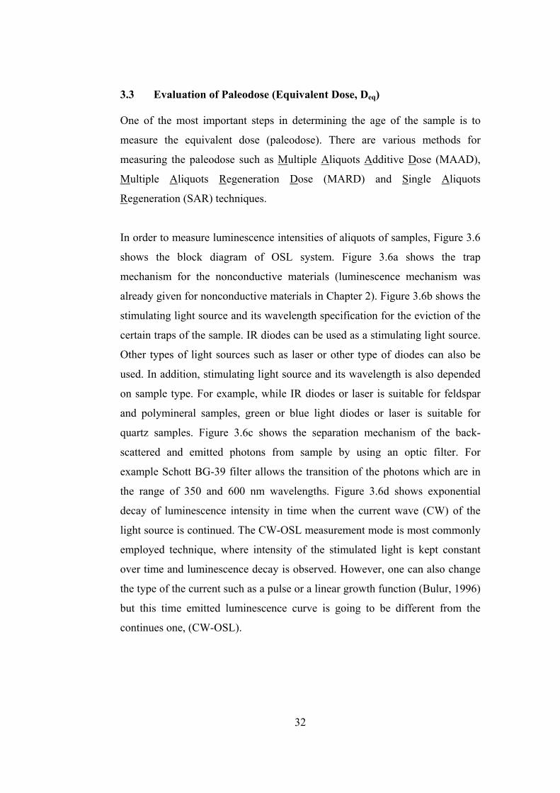
In order to measure luminescence intensities of aliquots of samples, Figure 3.6

shows the block diagram of OSL system. Figure 3.6a shows the trap

mechanism for the nonconductive materials (luminescence mechanism was

already given for nonconductive materials in Chapter 2). Figure 3.6b shows the

stimulating light source and its wavelength specification for the eviction of the

certain traps of the sample. IR diodes can be used as a stimulating light source.

Other types of light sources such as laser or other type of diodes can also be

used. In addition, stimulating light source and its wavelength is also depended

on sample type. For example, while IR diodes or laser is suitable for feldspar

and polymineral samples, green or blue light diodes or laser is suitable for

quartz samples. Figure 3.6c shows the separation mechanism of the back-

scattered and emitted photons from sample by using an optic filter. For

example Schott BG-39 filter allows the transition of the photons which are in

the range of 350 and 600 nm wavelengths. Figure 3.6d shows exponential

decay of luminescence intensity in time when the current wave (CW) of the

light source is continued. The CW-OSL measurement mode is most commonly

employed technique, where intensity of the stimulated light is kept constant

over time and luminescence decay is observed. However, one can also change

the type of the current such as a pulse or a linear growth function (Bulur, 1996)

but this time emitted luminescence curve is going to be different from the

continues one, (CW-OSL).

32

Photomultiplier

Sample

Luminescence (au) (d)

time

Figure 3.6 Block diagram of OSL system and luminescence measurement. (a) shows the mechanism of luminescence with band model, (b) shows the emitted photon spectrum range of the IR diodes, (c) shows the allowed transmitted photon (TP) spectrum range by the Schott BG-39 colour filter and (d) shows the decay of the luminescence signal (dating signal).

L

Defect centers

T E

Conduction Band

Valence Band diffusion hole

diffusion electron

L

T

Defect centers L

T

ionization

diffusion

release

Heator

lightlight En

ergy

IR Intensity (au) (b) (CW: Continues Wave)

800 9 nm)

00 λ (

TP Intensity (au) (c)

300 600 λ (nm)

Luminescence

IR diodes (light source) and incident beam

Color filter (Schott BG-39)

(a)

33

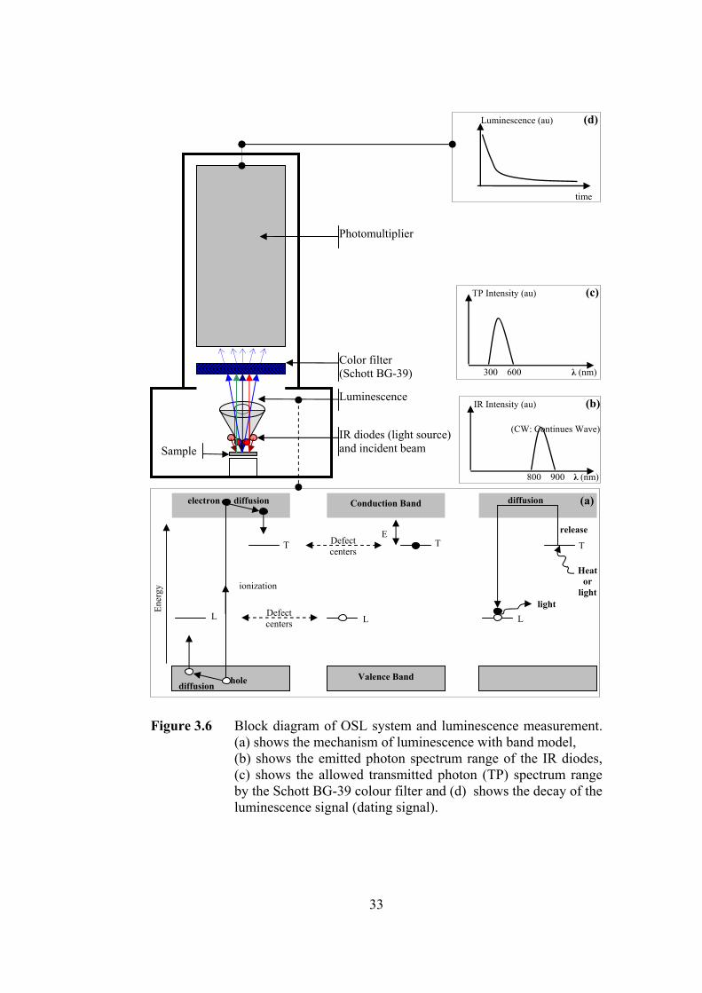
3.3.1 MAAD (Multiple Aliquots Additive Dose) Technique

The essential base of this method (alternatively, the additive-dose method, or,

the extrapolation method (MAAD)) is illustrated in Figure 3.7. A number of

equal portions-aliquots are prepared and divided into groups, with typically

half-a-dozen or more in each group. One group is reserved for measurement of

the natural OSL and the other groups are given various doses of laboratory

radiation before measurement, the same dose for each member of a group.

The luminescence intensity versus added dose graph is a straight line with

positive slope, as shown in Figure 3.7. The paleodose (or equivalent dose: Deq)

is determined from this graph by extrapolating the straight line to the horizontal

added dose axis. The intercept is equal to the paleodose Deq. The intensity of

luminescence emitted by each aliquot is determined by integrating its

luminescence decay curve (Figure 3.8).

N+D2

N+D1

N

0 D1 D2 D3 D4

N+D3

N+D4

Deq

Dose (Gy)

Luminescence (au)

Paleodose

Figure 3.7 Additive dose method of paleodose evaluation. Each data point is the average OSL from a group of aliquots, all members of each group have been given the same laboratory dose (except for the lowest point, N, for which the laboratory dose is zero). In the case shown the growth is linear with dose, i.e. a straight line is a good fit to the data points; the paleodose, Deq, is read off as the intercept on the dose axis.

34

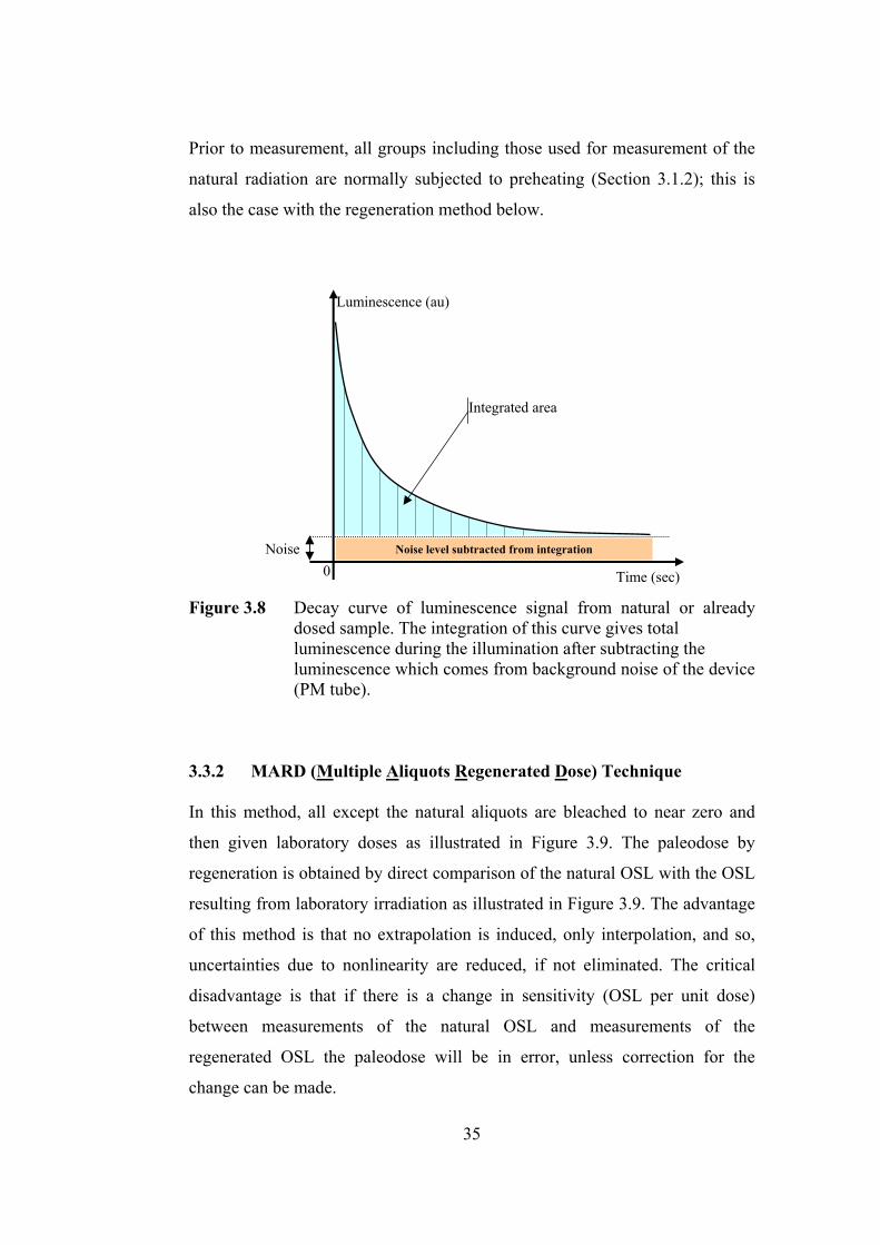
Prior to measurement, all groups including those used for measurement of the

natural radiation are normally subjected to preheating (Section 3.1.2); this is

also the case with the regeneration method below.

Time (sec)

Luminescence (au)

0 Noise Noise level subtracted from integration

Integrated area

Figure 3.8 Decay curve of luminescence signal from natural or already dosed sample. The integration of this curve gives total luminescence during the illumination after subtracting the luminescence which comes from background noise of the device (PM tube).

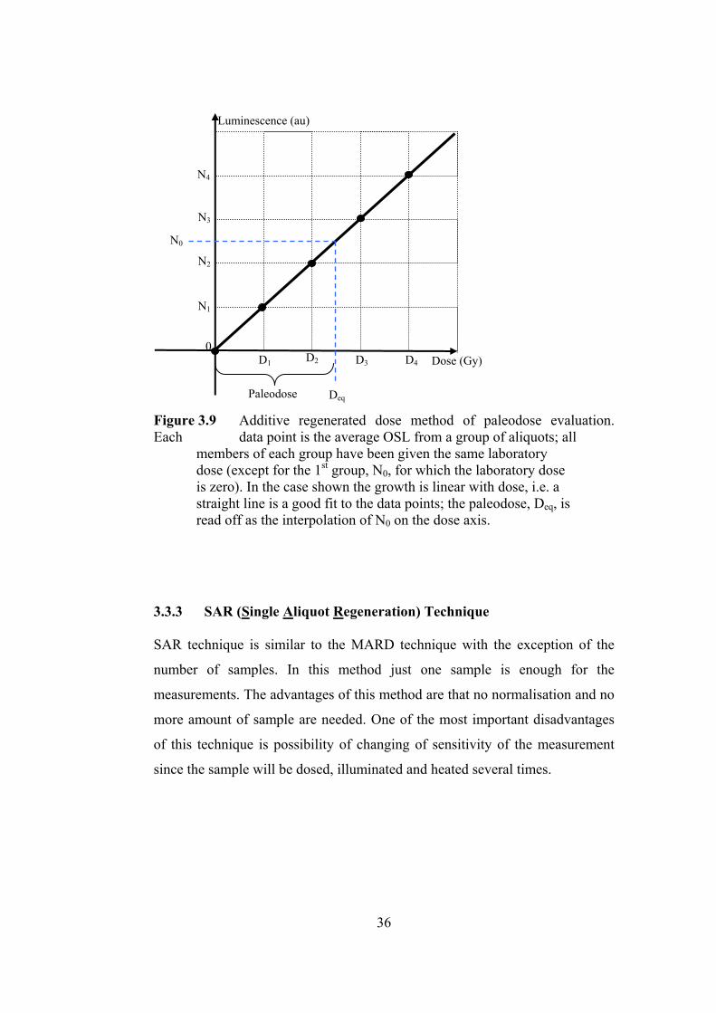
3.3.2 MARD (Multiple Aliquots Regenerated Dose) Technique

In this method, all except the natural aliquots are bleached to near zero and

then given laboratory doses as illustrated in Figure 3.9. The paleodose by

regeneration is obtained by direct comparison of the natural OSL with the OSL

resulting from laboratory irradiation as illustrated in Figure 3.9. The advantage

of this method is that no extrapolation is induced, only interpolation, and so,

uncertainties due to nonlinearity are reduced, if not eliminated. The critical

disadvantage is that if there is a change in sensitivity (OSL per unit dose)

between measurements of the natural OSL and measurements of the

regenerated OSL the paleodose will be in error, unless correction for the

change can be made.

35

N3

N2

N1

0D1 D2 D3 D4

N4

Deq

Dose (Gy)

Luminescence (au)

Paleodose

N0

Figure 3.9 Additive regenerated dose method of paleodose evaluation. Each data point is the average OSL from a group of aliquots; all members of each group have been given the same laboratory dose (except for the 1st group, N0, for which the laboratory dose is zero). In the case shown the growth is linear with dose, i.e. a straight line is a good fit to the data points; the paleodose, Deq, is read off as the interpolation of N0 on the dose axis.

3.3.3 SAR (Single Aliquot Regeneration) Technique

SAR technique is similar to the MARD technique with the exception of the

number of samples. In this method just one sample is enough for the

measurements. The advantages of this method are that no normalisation and no

more amount of sample are needed. One of the most important disadvantages

of this technique is possibility of changing of sensitivity of the measurement

since the sample will be dosed, illuminated and heated several times.

36

3.4 Preheating

In order to work with stable (deep) traps, unstable (shallow) traps must be

emptied. Deep traps are more stable than the shallow ones. Working on stable

traps is more convenient and better results can be obtained for dose

measurements. Therefore, electrons from the shallow traps must be removed.

The removal of the electrons from the shallow traps can be done by heating.

This process is called preheating. The preheating temperature and heating time

depend on the depths of the traps which will be emptied. Another correction

factor is normalization as explained below.

In general, preheating temperature and duration time for quartz is 48 hours at

150 oC (Wolfe et al., 1995), 16 hours at 160 oC (Stokes, 1992), 5 minutes at

220 oC (Rhodes, 1988 and 1990) and 1 minute at 240 oC (Franklin et al., 1995).

In addition, preheating temperature and duration time for feldspar is 2 hours at

160 oC (Aitken, 1998).

3.5 Normalisation

It is practically impossible to prepare identical aliquots of samples. Each

aliquot may be different from the others with respect to the amount of the

sample it contains. Furthermore, an aliquot may have grains of different size

and type. By doing a normalisation process, these differences may be taken

into account. For normalisation a relatively short shine (such as an IR shine for

0.1 s) is given to each aliquot before any additional dose (Aitken, 1985). After

the short shine the luminescence is measured for each aliquot and the average

luminescence L is calculated as

n), ......, , (in

LL

n

ii

21 1 ==∑= (3.2)

37

Where n is the number of aliquots and Li is the measured luminescence of the

ith aliquot. The normalisation constant Ci is defined as

ii L

LC = (3.3)

The normalised luminescence (NL)i for the ith aliquot is calculated as

iii L.C)NL( = (3.4)

The normalisation process requires the same short shine for all aliquots.

Ideally there should be no scatter in the normalized OSL from a group of

aliquots that have received the same dosing. In practice the scatter is often

quite substantial and it is uncommon for the standard deviation to be much

better than ±5 per cent (Aitken, 1998).

3.6 Sample Preparation

Sample preparation is another important step in OSL measurements. The fine

grain technique is used in order to include α-radiation contribution on natural

dose measurements. Since the α-radiation has extremely short range of travel in

pottery fabric (about 25 μm) grain size of the samples must be in the (1-9) μm

range. For such grains there is full penetration of α particles and the attenuation

of the α contribution is due to only its poor effectiveness (Aitken, 1998).

The mineralogical composition of each sample is generally determined using

the X-ray diffraction analysis (XRD).

38

3.7 Size distribution of the samples

In order to obtain fine grains (1-9 μm) powdered samples should be subjected

to the size distribution treatment and the size distribution is done in two ways;

1. by sieving the powdered dry sample with different sized screens,

2. by dispersing the powdered sample in a fluid and then by settling the

grains at different time periods according to Stoke’s law (Fleming, 1979).

3.8 Annual Dose Measurements

Naturally absorbed equivalent dose (paleodose) of the archaeological or

geological sample is due to the radioactive isotopes present within the sample

and in the surrounding soil. The internal radioactivity of the sample itself is

related to its U, Th and K content. These elements emit α, β particles and γ rays

(see Table 3.2). The same isotopes also exist in the soil around the sample and

this external radioactivity also contributes to the equivalent dose. Another

contribution is from the cosmic rays and their secondaries penetrating through

the soil and sample.

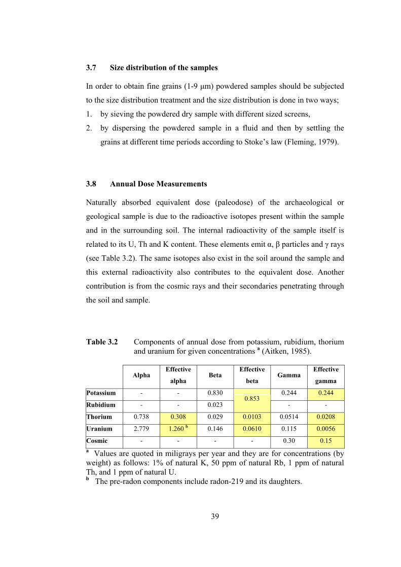
Table 3.2 Components of annual dose from potassium, rubidium, thorium and uranium for given concentrations a (Aitken, 1985).

Alpha Effective

alpha Beta

Effective

beta Gamma

Effective

gamma

Potassium - - 0.830 0.244 0.244

Rubidium - - 0.023 0.853

- -

Thorium 0.738 0.308 0.029 0.0103 0.0514 0.0208

Uranium 2.779 1.260 b 0.146 0.0610 0.115 0.0056

Cosmic - - - - 0.30 0.15 a Values are quoted in miligrays per year and they are for concentrations (by weight) as follows: 1% of natural K, 50 ppm of natural Rb, 1 ppm of natural Th, and 1 ppm of natural U. b The pre-radon components include radon-219 and its daughters.

39

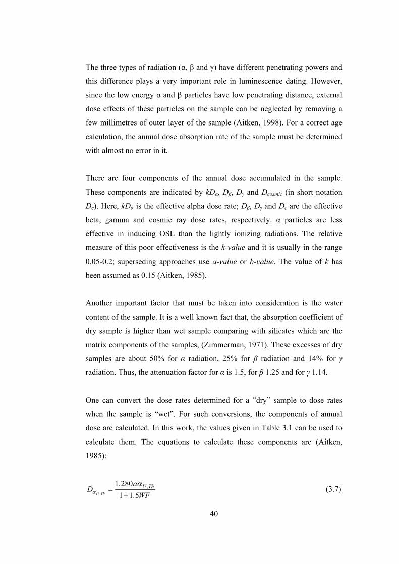
The three types of radiation (α, β and γ) have different penetrating powers and

this difference plays a very important role in luminescence dating. However,

since the low energy α and β particles have low penetrating distance, external

dose effects of these particles on the sample can be neglected by removing a

few millimetres of outer layer of the sample (Aitken, 1998). For a correct age

calculation, the annual dose absorption rate of the sample must be determined

with almost no error in it.

There are four components of the annual dose accumulated in the sample.

These components are indicated by kDα, Dβ, Dγ and Dcosmic (in short notation

Dc). Here, kDα is the effective alpha dose rate; Dβ, Dγ and Dc are the effective

beta, gamma and cosmic ray dose rates, respectively. α particles are less

effective in inducing OSL than the lightly ionizing radiations. The relative

measure of this poor effectiveness is the k-value and it is usually in the range

0.05-0.2; superseding approaches use a-value or b-value. The value of k has

been assumed as 0.15 (Aitken, 1985).

Another important factor that must be taken into consideration is the water

content of the sample. It is a well known fact that, the absorption coefficient of

dry sample is higher than wet sample comparing with silicates which are the

matrix components of the samples, (Zimmerman, 1971). These excesses of dry

samples are about 50% for α radiation, 25% for β radiation and 14% for γ

radiation. Thus, the attenuation factor for α is 1.5, for β 1.25 and for γ 1.14.

One can convert the dose rates determined for a “dry” sample to dose rates

when the sample is “wet”. For such conversions, the components of annual

dose are calculated. In this work, the values given in Table 3.1 can be used to

calculate them. The equations to calculate these components are (Aitken,

1985):

WF.a.

D Th,UTh,U 511

2801+

=α

α (3.7)

40

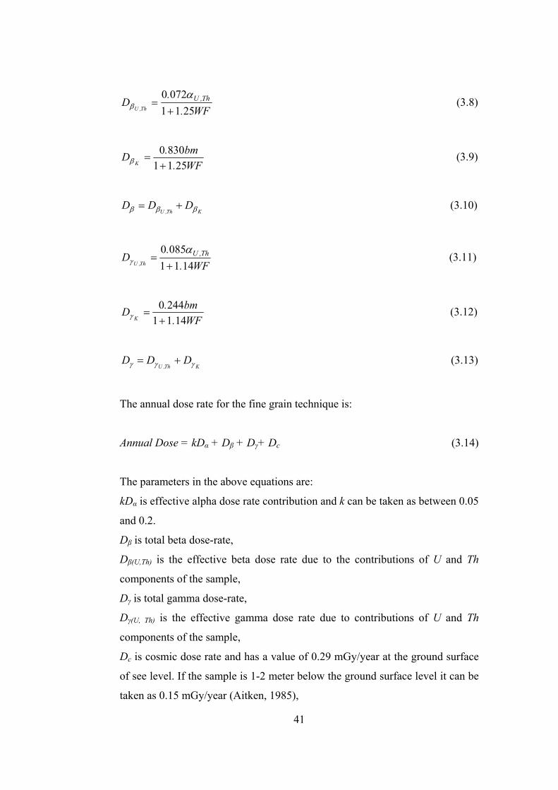
WF..

D Th,UTh,U 2511

0720+

=α

β (3.8)

WF.bm.D

K 25118300

+=β (3.9)

KTh,UDDD βββ += (3.10)

WF..

D Th,UTh,U 1411

0850+

=α

γ (3.11)

WF.bm.D

K 14112440

+=γ (3.12)

KTh,UDDD γγγ += (3.13)

The annual dose rate for the fine grain technique is:

Annual Dose = kDα + Dβ + Dγ+ Dc (3.14)

The parameters in the above equations are:

kDα is effective alpha dose rate contribution and k can be taken as between 0.05

and 0.2.

Dβ is total beta dose-rate,

Dβ(U,Th) is the effective beta dose rate due to the contributions of U and Th

components of the sample,

Dγ is total gamma dose-rate,

Dγ(U, Th) is the effective gamma dose rate due to contributions of U and Th

components of the sample,

Dc is cosmic dose rate and has a value of 0.29 mGy/year at the ground surface

of see level. If the sample is 1-2 meter below the ground surface level it can be

taken as 0.15 mGy/year (Aitken, 1985),

41

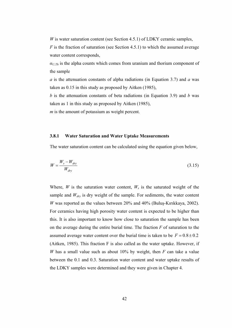
W is water saturation content (see Section 4.5.1) of LDKY ceramic samples,

F is the fraction of saturation (see Section 4.5.1) to which the assumed average

water content corresponds,

αU,Th is the alpha counts which comes from uranium and thorium component of

the sample

a is the attenuation constants of alpha radiations (in Equation 3.7) and a was

taken as 0.15 in this study as proposed by Aitken (1985),

b is the attenuation constants of beta radiations (in Equation 3.9) and b was

taken as 1 in this study as proposed by Aitken (1985),

m is the amount of potassium as weight percent.

3.8.1 Water Saturation and Water Uptake Measurements

The water saturation content can be calculated using the equation given below,

dry

drys

WWW

W−

= (3.15)

Where, W is the saturation water content, Ws is the saturated weight of the

sample and Wdry is dry weight of the sample. For sediments, the water content

W was reported as the values between 20% and 40% (Buluş-Kırıkkaya, 2002).

For ceramics having high porosity water content is expected to be higher than

this. It is also important to know how close to saturation the sample has been

on the average during the entire burial time. The fraction F of saturation to the

assumed average water content over the burial time is taken to be

(Aitken, 1985). This fraction F is also called as the water uptake. However, if

W has a small value such as about 10% by weight, then F can take a value

between the 0.1 and 0.3. Saturation water content and water uptake results of

the LDKY samples were determined and they were given in Chapter 4.

2080 ..F ±=

42

3.8.2 Determination of Potassium in Samples

Potassium-40 is naturally occurring radioactive isotope of potassium element.

Potassium is the seventh most abundant element in the earth’s crust and the

sixth most abundant element in the oceans. It is present in mineral waters,

brines, and in various minerals such as carnallite (KMgCl3.6H2O, Hydrated

Potassium Magnesium Chloride), feldspar (KAlSi3O8, Orthoclase or

Microcline), saltpetre (KNO3, potassium nitrate), glauconite

{K2(Mg,Fe)2Al6(Si4O10)3(OH)12}, and sylvite (KCl, Potassium Chloride).

Radioactive properties of potassium-40 are given in Table 3.3. K-40 emits β

radiation and captures electron and this radiations can cause electron trapping

in the crystal structure. Thus, K-40 gives two decay processes as shown in

Equations 3.16 and 3.17.

(3.16) β014020

894019 −+⎯⎯→⎯ CaK %

γ+⎯⎯→⎯+− AreK % 4018

1101

4019 (3.17)

Therefore, by the determination of the amount of potassium, it is possible to

calculate the contribution of β radiation coming from K-40 in the sample

irradiated.

43

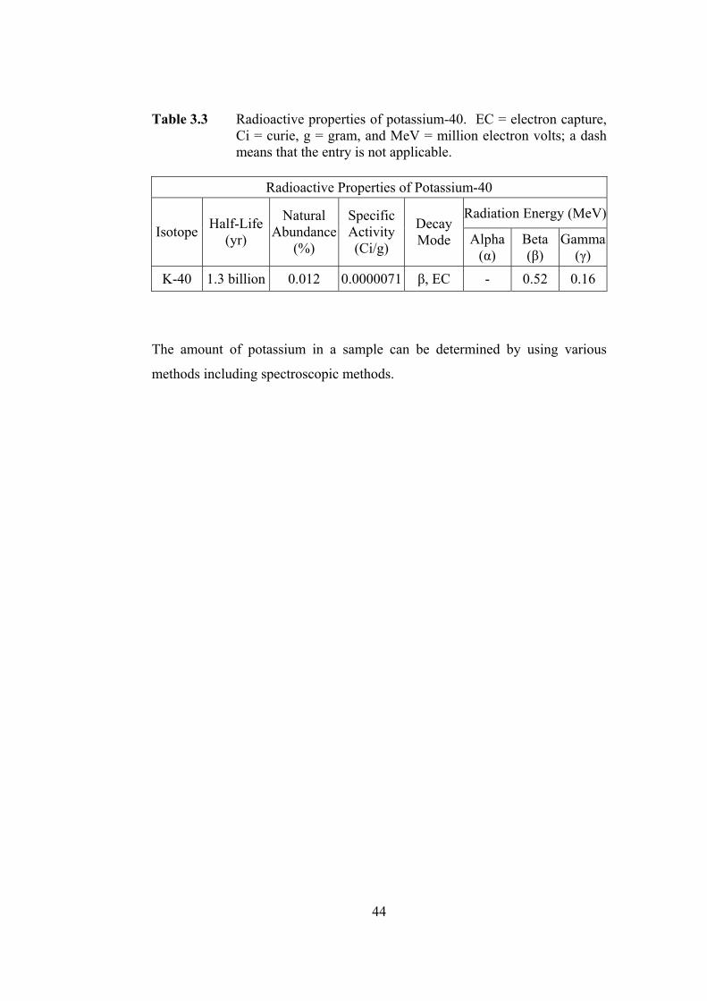
Table 3.3 Radioactive properties of potassium-40. EC = electron capture, Ci = curie, g = gram, and MeV = million electron volts; a dash means that the entry is not applicable.

Radioactive Properties of Potassium-40

Radiation Energy (MeV)Isotope Half-Life

(yr)

Natural Abundance

(%)

Specific Activity (Ci/g)

Decay Mode Alpha

(α) Beta (β)

Gamma (γ)

K-40 1.3 billion 0.012 0.0000071 β, EC - 0.52 0.16

The amount of potassium in a sample can be determined by using various

methods including spectroscopic methods.

44

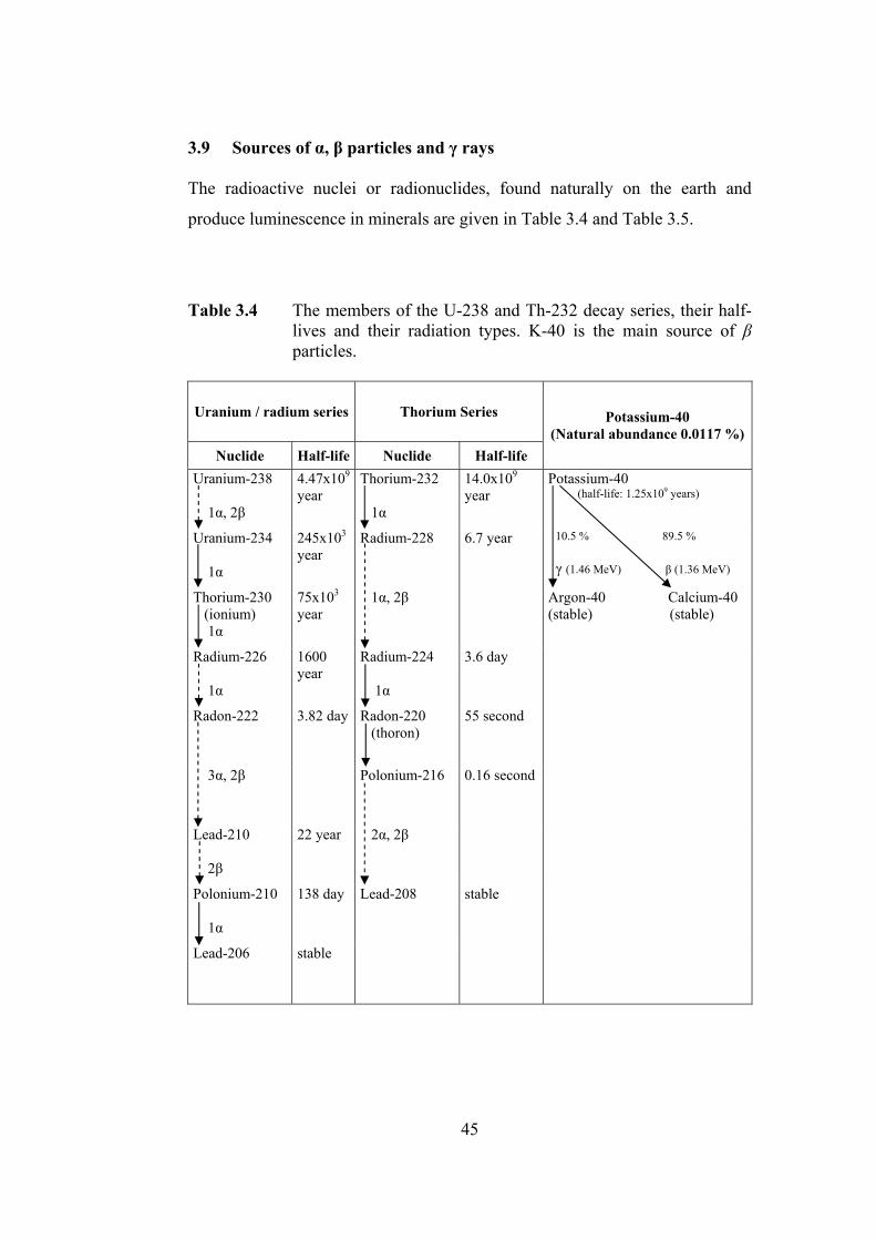
3.9 Sources of α, β particles and γ rays

The radioactive nuclei or radionuclides, found naturally on the earth and

produce luminescence in minerals are given in Table 3.4 and Table 3.5.

Table 3.4 The members of the U-238 and Th-232 decay series, their half- lives and their radiation types. K-40 is the main source of β particles.

Uranium / radium series Thorium Series

Nuclide Half-life Nuclide Half-life

Potassium-40 (Natural abundance 0.0117 %)

Uranium-238 1α, 2β

4.47x109 year

Thorium-232 1α

14.0x109 year

Potassium-40 (half-life: 1.25x109 years)

Uranium-234 1α

245x103 year

Radium-228 6.7 year 10.5 % 89.5 % γ (1.46 MeV) β (1.36 MeV)

Thorium-230 (ionium) 1α

75x103 year

1α, 2β Argon-40 Calcium-40 (stable) (stable)

Radium-226 1α

1600 year

Radium-224 1α

3.6 day

Radon-222 3.82 day Radon-220 (thoron)

55 second

3α, 2β Polonium-216 0.16 second

Lead-210 2β

22 year 2α, 2β

Polonium-210 1α

138 day Lead-208 stable

Lead-206 stable

45

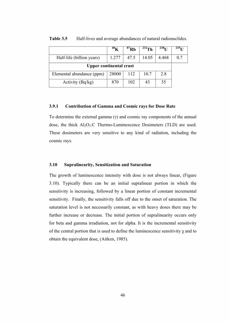
Table 3.5 Half-lives and average abundances of natural radionuclides.

40K 87Rb 232Th 238U 235U

Half-life (billion years) 1.277 47.5 14.05 4.468 0.7

Upper continental crust

Elemental abundance (ppm) 28000 112 10.7 2.8

Activity (Bq/kg) 870 102 43 35

3.9.1 Contribution of Gamma and Cosmic rays for Dose Rate

To determine the external gamma (γ) and cosmic ray components of the annual

dose, the thick Al2O3:C Thermo-Luminescence Dosimeters (TLD) are used.

These dosimeters are very sensitive to any kind of radiation, including the

cosmic rays.

3.10 Supralinearity, Sensitization and Saturation

The growth of luminescence intensity with dose is not always linear, (Figure

3.10). Typically there can be an initial supralinear portion in which the

sensitivity is increasing, followed by a linear portion of constant incremental

sensitivity. Finally, the sensitivity falls off due to the onset of saturation. The

saturation level is not necessarily constant, as with heavy doses there may be

further increase or decrease. The initial portion of supralinearity occurs only

for beta and gamma irradiation, not for alpha. It is the incremental sensitivity

of the central portion that is used to define the luminescence sensitivity χ and to

obtain the equivalent dose, (Aitken, 1985).

46

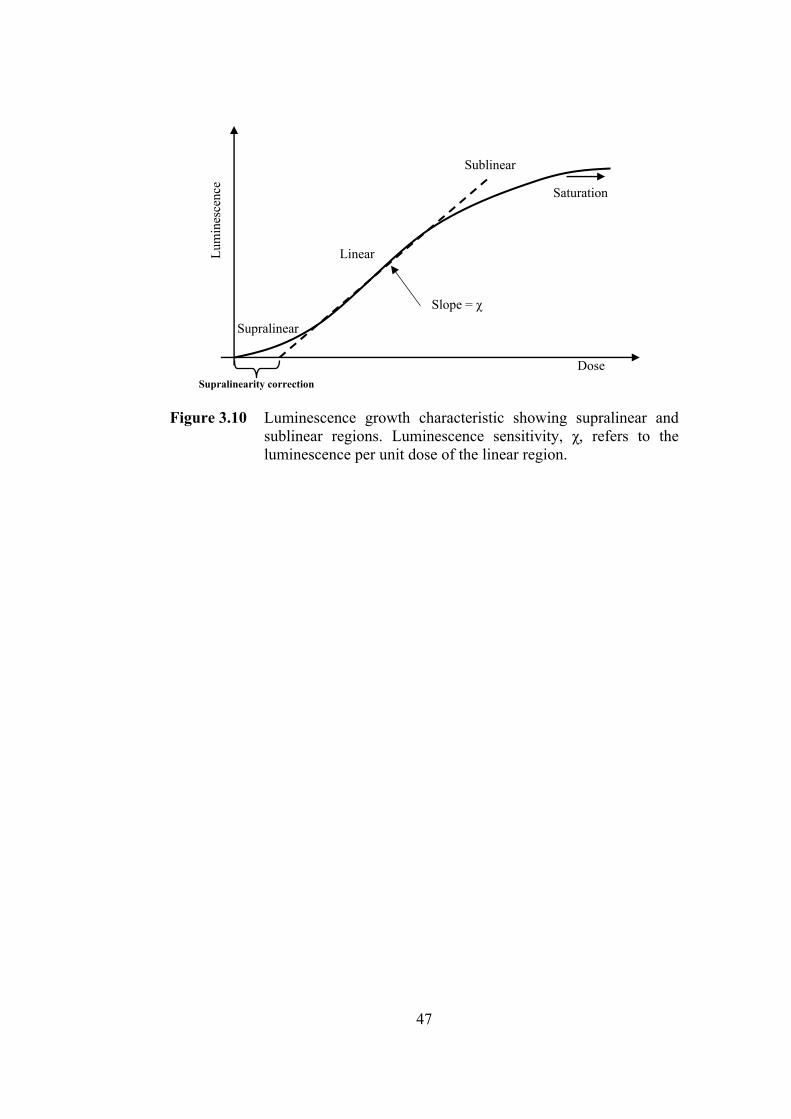
Linear

Sublinear

Saturation

Slope = χ

Supralinear

Dose

Lum

ines

cenc

e

Supralinearity correction

Figure 3.10 Luminescence growth characteristic showing supralinear and sublinear regions. Luminescence sensitivity, χ, refers to the luminescence per unit dose of the linear region.

47

CHAPTER 4

RESULTS and DISCUSSIONS

In order to reach the scope of the study and to increase the degree of sensitivity,

accuracy and reliability of the results, first of all calibrations of OSL (including

dose rate recalculation of Sr-90 β source) and Alpha counting systems have been

done. These studies are given in detail in Appendix B. Here, in Chapter 4 a very

brief summary of the work is given together with the discussion of the results.

The calibration of the ELSEC 9010 Optical Dating System has yielded the HT

and threshold voltages of PM tube as 1250±25 V and 3.30±0.01 V, respectively

(Tables B.1, B.2 and Figures B.2, B.3)

Dose rate calculations of Sr-90 β source have been carried out between the years

of 2001 and 2006 and a decrease of the activity in accordance with the decay

equation had been observed (Table B.6).

The HT and Threshold voltages of the Alpha Counter System were determined as

1150±25 V and 1.15±0.02 V, respectively (Tables B.3, B.4 and Figures B.5, B.6).

In order to determine radon escape, if there is, sealed and unsealed average alpha

count rates of the LDKY samples have been measured and the results were given

with their average U and Th contributions in Table 4.13.

In this study, samples of building materials (pieces of floor and ceiling tiles and

water pipes) collected from Laodikeia archaeological site (Denizli) were

48

examined. Mineral structure of the samples have analysed from their XRD traces

and results showed that the main minerals in the samples are quartz, feldspars

(dominantly potassium feldspar), calcite and together with some other minerals

(Figure 4.1).

Fine grained samples were prepared by the process given by Aitken (1985). For

the grain size distribution wet sieving method was preferred since the openings of

the sieves were filled by the particles in a short time in dry sieving. In the size

distribution, the Stoke’s law has been used and the fraction of (1-9) μm particles

were settled on the aluminium discs for measurements.

For the calculation of the age of the samples their equivalent dose and annual dose

have been determined. Before the calculation of equivalent dose, as a first step

preheating and then normalisation process were applied to the samples. There

after, two of the equivalent dose measurement techniques have been used.

Among the three methods mentioned in Chapter 3, MAAD and MARD techniques

were used for the equivalent dose measurements. SAR technique was not used

since the amount of samples is quite enough to use other two techniques. There

was no big difference between the results obtained which is in the range of 2.21-

6.30 Gy (Tables 4.3 and Table 4.10). This may be due to by two techniques for

the same sample studied.

Contributions of α, β particles, γ and cosmic rays and saturation water content had

been determined and from the annual dose equation the annual dose values of the

samples were calculated. The results are in the range of 2.35 and 4.03 mGy per

year, (Table 4.11).

The amount of water and humidity of material can affect the absorbed radiation

amount because of the attenuation differences of the radiation inside the sample.

Thus, water saturation content (W) should be determined and water uptake (F)

49

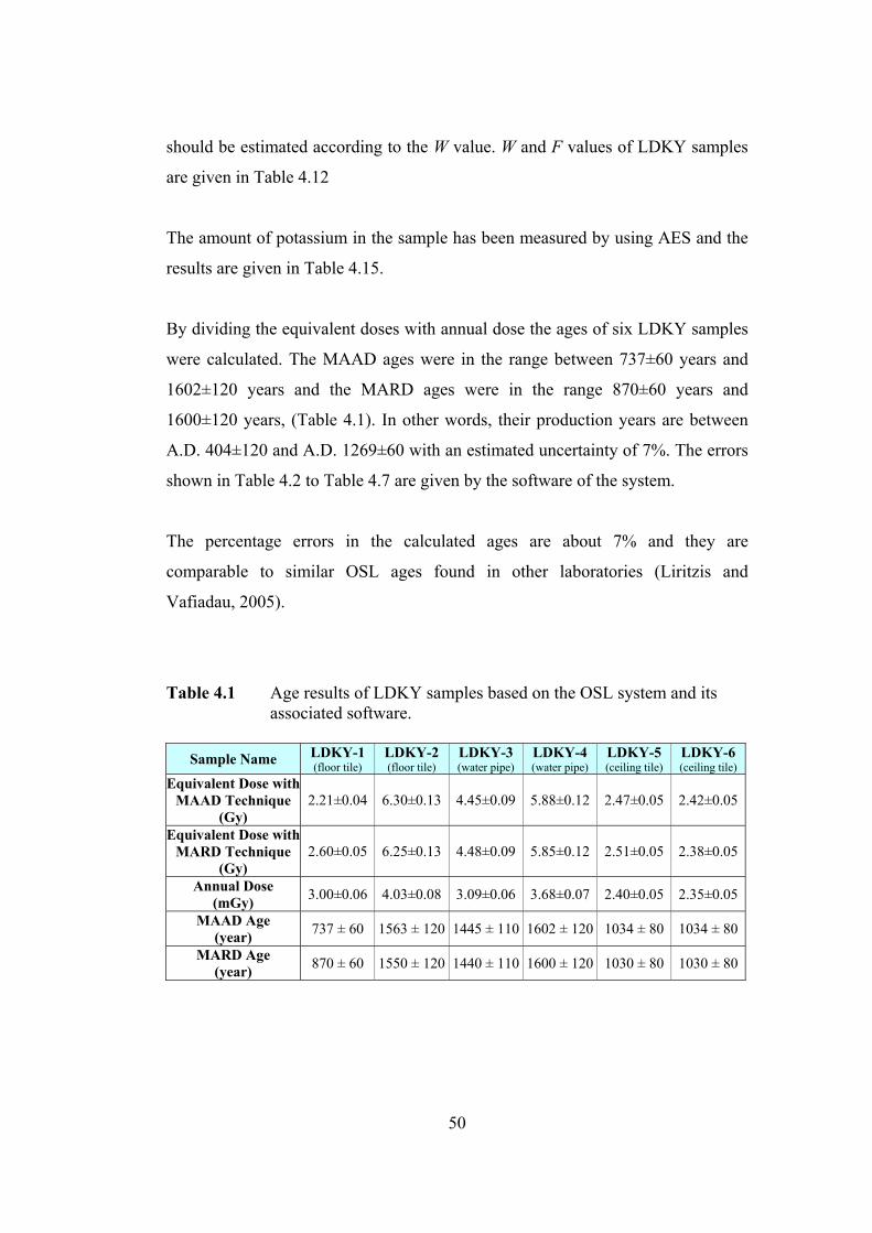
should be estimated according to the W value. W and F values of LDKY samples

are given in Table 4.12

The amount of potassium in the sample has been measured by using AES and the

results are given in Table 4.15.

By dividing the equivalent doses with annual dose the ages of six LDKY samples

were calculated. The MAAD ages were in the range between 737±60 years and

1602±120 years and the MARD ages were in the range 870±60 years and

1600±120 years, (Table 4.1). In other words, their production years are between

A.D. 404±120 and A.D. 1269±60 with an estimated uncertainty of 7%. The errors

shown in Table 4.2 to Table 4.7 are given by the software of the system.

The percentage errors in the calculated ages are about 7% and they are

comparable to similar OSL ages found in other laboratories (Liritzis and

Vafiadau, 2005).

Table 4.1 Age results of LDKY samples based on the OSL system and its associated software.

Sample Name LDKY-1 (floor tile)

LDKY-2 (floor tile)

LDKY-3 (water pipe)

LDKY-4 (water pipe)

LDKY-5 (ceiling tile)

LDKY-6 (ceiling tile)

Equivalent Dose with MAAD Technique

(Gy) 2.21±0.04 6.30±0.13 4.45±0.09 5.88±0.12 2.47±0.05 2.42±0.05

Equivalent Dose with MARD Technique

(Gy) 2.60±0.05 6.25±0.13 4.48±0.09 5.85±0.12 2.51±0.05 2.38±0.05

Annual Dose (mGy) 3.00±0.06 4.03±0.08 3.09±0.06 3.68±0.07 2.40±0.05 2.35±0.05

MAAD Age (year) 737 ± 60 1563 ± 120 1445 ± 110 1602 ± 120 1034 ± 80 1034 ± 80

MARD Age (year) 870 ± 60 1550 ± 120 1440 ± 110 1600 ± 120 1030 ± 80 1030 ± 80

50

The ages of the floor tiles “LDKY-1 and LDKY-2” have been found to be 870±60

years (Table 4.2) and 1550±120 years (Table 4.3) by MARD technique,

respectively. These floor tiles had been collected from the same room but at

different parts of it. The room is at the right side of the entrance door of the

Laodikeia church (Figures 3.1a and 3.1b). However, before they were collected

the roof had been already removed and the samples had been exposed to the

sunlight. Two different floor tiles were collected from that room. First sample

(LDKY-1) had been illuminated by the sun light for a couple of weeks but second

sample (LDKY-2) was not, because that tile was found underground in front of

the wall of the room (Figures 3.1a and 3.1b). Archaeologists were interested in the

construction date of the room. The age of LDKY-1 was found to be younger than

LDKY-2. This is an expected result since some of the traps were emptied by

sunlight.

The age of the second sample (LDKY-2) gives us the construction date of the

room, since it was not exposed to the sun light until it was collected. This is an

expected age by the archaeologists of Laodikeia excavation (Şimşek, 2004).

The ages of the water pipe samples, LDKY-3 and LDKY-4, have been found to be

1440±110 years (Table 4.4) and 1600±120 years (Table 4.5) by MARD technique,

respectively. These samples had been collected at the side of the north wall of the

Laodikeia church (Figures 3.2a and 3.2b).

The archaeologists claimed that the earthquake, which happened in A.D. 494

according to the archaeological written records, destroyed Laodikeia completely

and the city was reconstructed. So, LDKY-3 and LDKY-4 samples are expected

to give a date indicating this earthquake.

Consequently, the dates determined in this work for LDKY-3 and LDKY-4

samples are completely consistent with the earthquake date. This may indicate

that water pipes were made just after the devastating earthquake in A.D. 494.

51

The ages of the ceiling tile samples, LDKY-5 and LDKY-6, were found to be

1030±80 years (Tables 4.6) and 1030±80 years (Tables 4.7) by MARD technique,

respectively. These samples had been collected from the entrance door of the

Laodikeia church, one above the burnt layer and the other below this layer

(Figures 3.3a and 3.3b). According to the archaeologists, probably the ceiling of

the church was wooden and the top of it had been covered with the ceramic

ceiling tiles. In the fire this wooden ceiling were burnt and collapsed with the

ceramic tiles on it. According to the archaeologists, this fire had been set up

during the invasion of Seljuks, in A.D. 1176. So, the date of LDKY-5 and LDKY-

6 samples could be comparable with this invasion date, and the fire has been acted

as a zeroing event.

The glow curve of the LDKY samples has not shown any supralinearity, (Figure

4.14). The sensitivities were constant, for all LDKY samples. For LDKY ceramic

samples studied, sublinearity started after 500 Gy, (Figure 4.14). This shows that

ceramic is a good natural dosimeter and age estimation can be done up to 100-150

kyear without making any supralinearity correction.

In this work preheating temperature for LDKY samples was determined to be 160

degrees of Celsius with 20 minutes duration time (Figure 4.3). In addition,

removal dose rate of the shallow traps was 30-35% of the total dose before

preheating applied on the LDKY aliquots. This result may show that the future

OSL analysis of other LDKY samples can be done by directly subtracting 30-35

% of the total luminescence for the shallow traps without preheating.

52

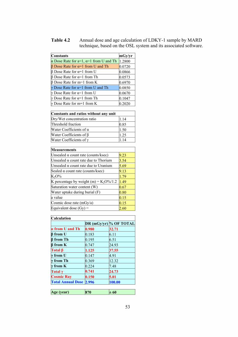
Table 4.2 Annual dose and age calculation of LDKY-1 sample by MARD technique, based on the OSL system and its associated software. Constants mGy/yr α Dose Rate for a=1, α=1 from U and Th 1.2800 β Dose Rate for α=1 from U and Th 0.0720 β Dose Rate for α=1 from U 0.0866 β Dose Rate for α=1 from Th 0.0573 β Dose Rate for m=1 from K 0.6970 γ Dose Rate for α=1 from U and Th 0.0850 γ Dose Rate for α=1 from U 0.0670 γ Dose Rate for α=1 from Th 0.1047 γ Dose Rate for m=1 from K 0.2020 Constants and ratios without any unit Dry/Wet concentration ratio 1.14 Threshold fraction 0.85 Water Coefficients of α 1.50 Water Coefficients of β 1.25 Water Coefficients of γ 1.14 Measurements Unsealed α count rate (counts/ksec) 9.23 Unsealed α count rate due to Thorium 3.54 Unsealed α count rate due to Uranium 5.69 Sealed α count rate (counts/ksec) 9.13 K2O% 1.79 K percentage by weight (m) = K2O%/1.2 1.49 Saturation water content (W) 0.67 Water uptake during burial (F) 0.80 a value 0.15 Cosmic dose rate (mGy/a) 0.15 Equivalent dose (Gy) = 2.60 Calculation DR (mGy/yr) % OF TOTALα from U and Th 0.980 32.71 β from U 0.183 6.11 β from Th 0.195 6.51 β from K 0.747 24.93 Total β 1.125 37.55 γ from U 0.147 4.91 γ from Th 0.369 12.32 γ from K 0.224 7.48 Total γ 0.741 24.73 Cosmic Ray 0.150 5.01 Total Annual Dose 2.996 100.00 Age (year) 870 ± 60

53

Table 4.3 Annual dose and age calculations of LDKY-2 sample by MARD technique, based on the OSL system and its associated software.

Constants mGy/yr α Dose Rate for a=1, α=1 from U and Th 1.2800 β Dose Rate for α=1 from U and Th 0.0720 β Dose Rate for α=1 from U 0.0866 β Dose Rate for α=1 from Th 0.0573 β Dose Rate for m=1 from K 0.6970 γ Dose Rate for α=1 from U and Th 0.0850 γ Dose Rate for α=1 from U 0.0670 γ Dose Rate for α=1 from Th 0.1047 γ Dose Rate for m=1 from K 0.2020 Constants and ratios without any unit Dry/Wet concentration ratio 1.14 Threshold fraction 0.85 Water Coefficients of α 1.50 Water Coefficients of β 1.25 Water Coefficients of γ 1.14 Measurements Unsealed α count rate (counts/ksec) 11.05 Unsealed α count rate due to Thorium 7.72 Unsealed α count rate due to Uranium 3.33 Sealed α count rate (counts/ksec) 11.31 K2O% 1.38 K percentage by weight (m) = K2O%/1.2 1.15 Saturation water content (W) 0.60 Water uptake during burial (F) 0.40 a value 0.15 Cosmic dose rate (mGy/a) 0.15 Equivalent dose (Gy) = 6.30 Calculation DR (mGy/yr) % OF TOTALα from U and Th 1.568 38.99 β from U 0.517 12.85 β from Th 0.147 3.65 β from K 0.740 18.40 Total β 1.404 34.91 γ from U 0.406 10.09 γ from Th 0.275 6.84 γ from K 0.219 5.45 Total γ 0.900 22.38 Cosmic Ray 0.150 3.73 Total Annual Dose 4.022 100.00 Age (year) 1550 ± 120

54

Table 4.4 Annual dose and age calculations of LDKY-3 sample by MARD technique, based on the OSL system and its associated software.

Constants mGy/yr α Dose Rate for a=1, α=1 from U and Th 1.2800 β Dose Rate for α=1 from U and Th 0.0720 β Dose Rate for α=1 from U 0.0866 β Dose Rate for α=1 from Th 0.0573 β Dose Rate for m=1 from K 0.6970 γ Dose Rate for α=1 from U and Th 0.0850 γ Dose Rate for α=1 from U 0.0670 γ Dose Rate for α=1 from Th 0.1047 γ Dose Rate for m=1 from K 0.2020 Constants and ratios without any unit Dry/Wet concentration ratio 1.14 Threshold fraction 0.85 Water Coefficients of α 1.50 Water Coefficients of β 1.25 Water Coefficients of γ 1.14 Measurements Unsealed α count rate (counts/ksec) 10.85 Unsealed α count rate due to Thorium 4.52 Unsealed α count rate due to Uranium 6.33 Sealed α count rate (counts/ksec) 11.02 K2O% 0.85 K percentage by weight (m) = K2O%/1.2 0.71 Saturation water content (W) 0.70 Water uptake during burial (F) 0.60 a value 0.15 Cosmic dose rate (mGy/a) 0.15 Equivalent dose (Gy) = 4.45 Calculation DR (mGy/yr) % OF TOTALα from U and Th 1.282 41.52 β from U 0.258 8.35 β from Th 0.239 7.74 β from K 0.388 12.56 Total β 0.885 28.66 γ from U 0.205 6.64 γ from Th 0.450 14.57 γ from K 0.116 3.76 Total γ 0.771 24.97 Cosmic Ray 0.150 4.86 Total Annual Dose 3.088 100.00 Age (year) 1440 ± 110

55

Table 4.5 Annual dose and age calculations of LDKY-4 sample by MARD technique, based on the OSL system and its associated software.

Constants mGy/yr α Dose Rate for a=1, α=1 from U and Th 1.2800 β Dose Rate for α=1 from U and Th 0.0720 β Dose Rate for α=1 from U 0.0866 β Dose Rate for α=1 from Th 0.0573 β Dose Rate for m=1 from K 0.6970 γ Dose Rate for α=1 from U and Th 0.0850 γ Dose Rate for α=1 from U 0.0670 γ Dose Rate for α=1 from Th 0.1047 γ Dose Rate for m=1 from K 0.2020 Constants and ratios without any unit Dry/Wet concentration ratio 1.14 Threshold fraction 0.85 Water Coefficients of α 1.50 Water Coefficients of β 1.25 Water Coefficients of γ 1.14 Measurements Unsealed α count rate (counts/ksec) 8.53 Unsealed α count rate due to Thorium 3.64 Unsealed α count rate due to Uranium 4.89 Sealed α count rate (counts/ksec) 8.77 K2O% 0.69 K percentage by weight (m) = K2O%/1.2 0.57 Saturation water content (W) 0.10 Water uptake during burial (F) 0.20 a value 0.15 Cosmic dose rate (mGy/a) 0.15 Equivalent dose (Gy) = 5.88 Calculation DR (mGy/yr) % OF TOTALα from U and Th 1.600 43.45 β from U 0.309 8.40 β from Th 0.275 7.46 β from K 0.469 12.75 Total β 1.053 28.61 γ from U 0.239 6.48 γ from Th 0.503 13.67 γ from K 0.136 3.70 Total γ 0.878 23.86 Cosmic Ray 0.150 4.07 Total Annual Dose 3.681 100.00 Age (year) 1600 ± 120

56

Table 4.6 Annual dose and age calculations of LDKY-5 sample by MARD technique, based on the OSL system and its associated software.

Constants mGy/yr α Dose Rate for a=1, α=1 from U and Th 1.2800 β Dose Rate for α=1 from U and Th 0.0720 β Dose Rate for α=1 from U 0.0866 β Dose Rate for α=1 from Th 0.0573 β Dose Rate for m=1 from K 0.6970 γ Dose Rate for α=1 from U and Th 0.0850 γ Dose Rate for α=1 from U 0.0670 γ Dose Rate for α=1 from Th 0.1047 γ Dose Rate for m=1 from K 0.2020 Constants and ratios without any unit Dry/Wet concentration ratio 1.14 Threshold fraction 0.85 Water Coefficients of α 1.50 Water Coefficients of β 1.25 Water Coefficients of γ 1.14 Measurements Unsealed α count rate (counts/ksec) 8.77 Unsealed α count rate due to Thorium 3.60 Unsealed α count rate due to Uranium 5.17 Sealed α count rate (counts/ksec) 9.80 K2O% 0.85 K percentage by weight (m) = K2O%/1.2 0.71 Saturation water content (W) 0.69 Water uptake during burial (F) 0.80 a value 0.15 Cosmic dose rate (mGy/a) 0.15 Equivalent dose (Gy) = 2.47 Calculation DR (mGy/yr) % OF TOTALα from U and Th 0.944 39.22 β from U 0.189 7.85 β from Th 0.179 7.44 β from K 0.351 14.58 Total β 0.719 29.87 γ from U 0.148 6.15 γ from Th 0.340 14.13 γ from K 0.105 4.36 Total γ 0.594 24.68 Cosmic Ray 0.150 6.23 Total Annual Dose 2.407 100.00 Age (year) 1030 ± 80

57

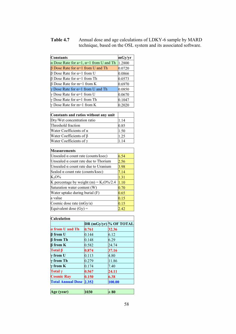
Table 4.7 Annual dose and age calculations of LDKY-6 sample by MARD technique, based on the OSL system and its associated software.

Constants mGy/yr α Dose Rate for a=1, α=1 from U and Th 1.2800 β Dose Rate for α=1 from U and Th 0.0720 β Dose Rate for α=1 from U 0.0866 β Dose Rate for α=1 from Th 0.0573 β Dose Rate for m=1 from K 0.6970 γ Dose Rate for α=1 from U and Th 0.0850 γ Dose Rate for α=1 from U 0.0670 γ Dose Rate for α=1 from Th 0.1047 γ Dose Rate for m=1 from K 0.2020 Constants and ratios without any unit Dry/Wet concentration ratio 1.14 Threshold fraction 0.85 Water Coefficients of α 1.50 Water Coefficients of β 1.25 Water Coefficients of γ 1.14 Measurements Unsealed α count rate (counts/ksec) 6.54 Unsealed α count rate due to Thorium 2.56 Unsealed α count rate due to Uranium 3.98 Sealed α count rate (counts/ksec) 7.14 K2O% 1.31 K percentage by weight (m) = K2O%/2.4 1.10 Saturation water content (W) 0.70 Water uptake during burial (F) 0.65 a value 0.15 Cosmic dose rate (mGy/a) 0.15 Equivalent dose (Gy) = 2.42 Calculation DR (mGy/yr) % OF TOTALα from U and Th 0.761 32.36 β from U 0.144 6.12 β from Th 0.148 6.29 β from K 0.582 24.74 Total β 0.874 37.16 γ from U 0.113 4.80 γ from Th 0.279 11.86 γ from K 0.174 7.40 Total γ 0.567 24.11 Cosmic Ray 0.150 6.38 Total Annual Dose 2.352 100.00 Age (year) 1030 ± 80

58

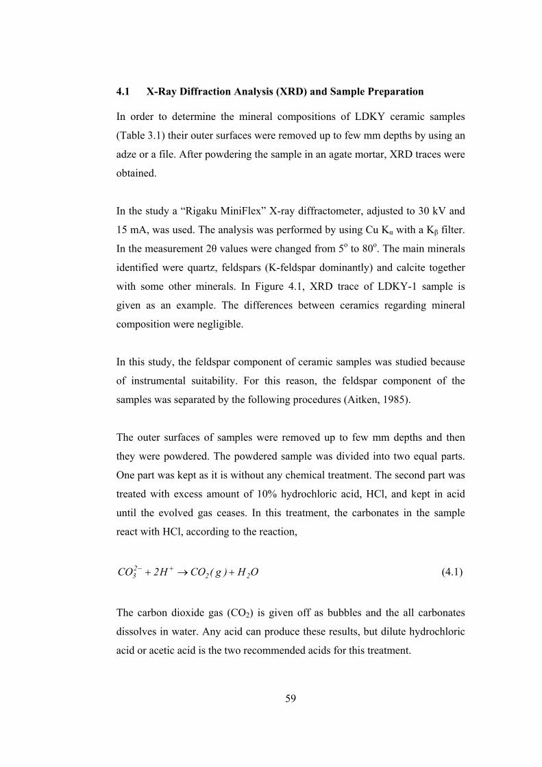
4.1 X-Ray Diffraction Analysis (XRD) and Sample Preparation

In order to determine the mineral compositions of LDKY ceramic samples

(Table 3.1) their outer surfaces were removed up to few mm depths by using an

adze or a file. After powdering the sample in an agate mortar, XRD traces were

obtained.

In the study a “Rigaku MiniFlex” X-ray diffractometer, adjusted to 30 kV and

15 mA, was used. The analysis was performed by using Cu Kα with a Kβ filter.

In the measurement 2θ values were changed from 5o to 80o. The main minerals

identified were quartz, feldspars (K-feldspar dominantly) and calcite together

with some other minerals. In Figure 4.1, XRD trace of LDKY-1 sample is

given as an example. The differences between ceramics regarding mineral

composition were negligible.

In this study, the feldspar component of ceramic samples was studied because

of instrumental suitability. For this reason, the feldspar component of the

samples was separated by the following procedures (Aitken, 1985).

The outer surfaces of samples were removed up to few mm depths and then

they were powdered. The powdered sample was divided into two equal parts.

One part was kept as it is without any chemical treatment. The second part was

treated with excess amount of 10% hydrochloric acid, HCl, and kept in acid

until the evolved gas ceases. In this treatment, the carbonates in the sample

react with HCl, according to the reaction,

OH)g(COH2CO 2223 +→+ +− (4.1)

The carbon dioxide gas (CO2) is given off as bubbles and the all carbonates

dissolves in water. Any acid can produce these results, but dilute hydrochloric

acid or acetic acid is the two recommended acids for this treatment.

59

60

At the end of this process, the suspension is kept aside to settle down all the

undissolved components. Then, the supernatant solution was decanted. The

remaining residue was rinsed with distilled water for several times to be sure

the residue became clean. Then, the sample was treated with excess amount of

38% H2O2 to remove any organic matter and keep waiting until the evolved gas

ceases, and the suspension is kept aside to settle down all the undissolved

components. Then, the supernatant solution was decanted. The remaining

residue was rinsed with distilled water for several times. Rinsing process was

repeated by adding acetone last time for the final process to remove all

chemical impurities. So the samples became ready for size distribution analysis

after drying for all dose measurements.

The XRD trace of treated sample was taken which is shown in Figure 4.1b.

As it is seen in Figure 4.1b, some of the calcite peaks observed clearly in

untreated sample, Figure 4.1a, were decreased after the treatment of the sample

with HCl and H2O2.

61

Figure 4.1 XRD analysis of LDKY1 ceramic sample. a) Untreated (red line), b) Treated sample (blue line) with HCl and H2O2. Where, Q: quartz, F: feldspar, C: calcite.

500100015002000250030003500

20 25 30 35 40 45 50 55 60 65 70

500100015002000250030003500

20 25 30 35 40 45 50 55 60 65 702θ Angle

I n t

e n

s i t

y (c

ps)

a

b

C Q

Q, F

F F

Q, F Q, F C Q, C C

C

61

4.1.1 Size distribution of the samples

In order to obtain fine grains (1-9 μm) powdered samples should be subjected to

the size distribution treatment and the size distribution is done in two ways;

1. by sieving the powdered dry sample with different sized screens,

2. by dispersing the powdered sample in a fluid and then by settling the grains at

different time periods according to Stoke’s law (Fleming 1979).

Dry sieving method is not found sufficient since the openings of the sieve will be

filled by the particles in a short time and the fine grains tended to conglomerate.

In the second method, the sample is dispersed in a solvent like acetone and a

uniform suspension is obtained. The suspension is kept aside until the particles in

it settle down under the action of gravity. Stoke’s law gives the settling speed of a

particle dropped into a fluid as

⎥⎦

⎤⎢⎣

⎡ −=

μρρ 2

181 gd)(v Fs (4.2)

where,

v : settling speed (cm/s)

g : gravitational acceleration (g = 980 cm/s2)

ρs : density of dropped object (if feldspar is used density of feldspar :

2.55-2.76 gr/cm3, Cornelius and Hurlbut, 1971)

d : diameter of particle (assumed to be (2-9)x10-4 cm)

ρF : density of fluid (density of acetone = 0.79 gr/cm3)

μ : viscosity of fluid (viscosity of acetone = 0.0032 gr.cm-1.s-1).

The time t it takes a particle to go down a vertical distance h in the suspension is

given by

62

vht = (4.3)

After size distribution treatment, samples are placed on the aluminium discs in

equal amount of about 1 mgr/cm2. Then, paleodose measurements can be carried

out.

If the values given above are substituted in Equation 4.2 and Equation 4.3, t is

found as 120 seconds for the particles to settle down in a 6-cm suspension height

formed in a 3.5-cm diameter graduated cylinder.

In the method used, 5-10 gr of powdered sample was dispersed in 100 ml of

acetone and a stock suspension was prepared. From this stock suspension, about

30 ml suspension is poured into a graduated cylinder and a 6-cm suspension

height is obtained. The suspension is settled for 2 minutes to settle out the grains

with diameters larger than 9 μm (as obtained from Stoke’s law). The supernatant

solution is decanted to another graduated cylinder and allowed for 20 minutes to

settle down the grains with diameters larger than 2.5 μm.

After decantation of supernatant solution, the grains with diameters between 2.5

μm and 9 μm are taken out and are put into sufficient amount of acetone to

produce homogeneous suspension and this is a new stock suspension is prepared

This homogenous suspension is poured, in equal amounts, to 30 small, flat-

bottomed tubes, each with a thin aluminium disc located at the bottom. Then these

tubes are inserted in an oven at 50 oC to evaporate acetone. By this way a series of

individual aluminium discs, each with a layer of sample grains is obtained. Each

aluminium disc with sample on it is called aliquot. It was estimated that each

aluminium disc had about 1 mg/cm2 of grains on it.

63

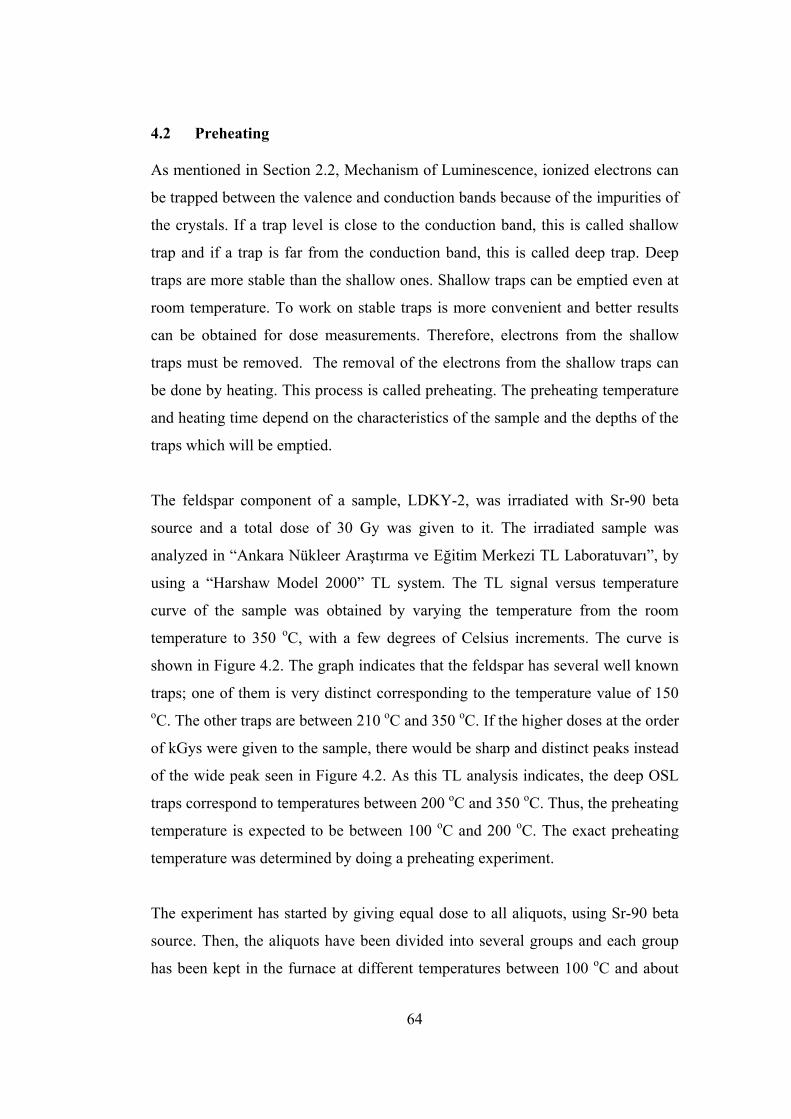
4.2 Preheating

As mentioned in Section 2.2, Mechanism of Luminescence, ionized electrons can

be trapped between the valence and conduction bands because of the impurities of

the crystals. If a trap level is close to the conduction band, this is called shallow

trap and if a trap is far from the conduction band, this is called deep trap. Deep

traps are more stable than the shallow ones. Shallow traps can be emptied even at

room temperature. To work on stable traps is more convenient and better results

can be obtained for dose measurements. Therefore, electrons from the shallow

traps must be removed. The removal of the electrons from the shallow traps can

be done by heating. This process is called preheating. The preheating temperature

and heating time depend on the characteristics of the sample and the depths of the

traps which will be emptied.

The feldspar component of a sample, LDKY-2, was irradiated with Sr-90 beta

source and a total dose of 30 Gy was given to it. The irradiated sample was

analyzed in “Ankara Nükleer Araştırma ve Eğitim Merkezi TL Laboratuvarı”, by

using a “Harshaw Model 2000” TL system. The TL signal versus temperature

curve of the sample was obtained by varying the temperature from the room

temperature to 350 oC, with a few degrees of Celsius increments. The curve is

shown in Figure 4.2. The graph indicates that the feldspar has several well known

traps; one of them is very distinct corresponding to the temperature value of 150 oC. The other traps are between 210 oC and 350 oC. If the higher doses at the order

of kGys were given to the sample, there would be sharp and distinct peaks instead

of the wide peak seen in Figure 4.2. As this TL analysis indicates, the deep OSL

traps correspond to temperatures between 200 oC and 350 oC. Thus, the preheating

temperature is expected to be between 100 oC and 200 oC. The exact preheating

temperature was determined by doing a preheating experiment.

The experiment has started by giving equal dose to all aliquots, using Sr-90 beta

source. Then, the aliquots have been divided into several groups and each group

has been kept in the furnace at different temperatures between 100 oC and about

64

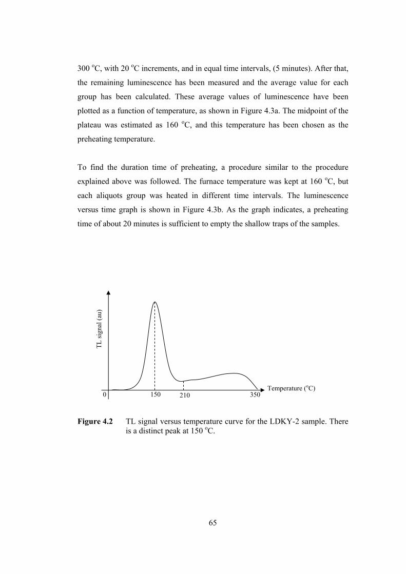
300 oC, with 20 oC increments, and in equal time intervals, (5 minutes). After that,

the remaining luminescence has been measured and the average value for each

group has been calculated. These average values of luminescence have been

plotted as a function of temperature, as shown in Figure 4.3a. The midpoint of the

plateau was estimated as 160 oC, and this temperature has been chosen as the

preheating temperature.

To find the duration time of preheating, a procedure similar to the procedure

explained above was followed. The furnace temperature was kept at 160 oC, but

each aliquots group was heated in different time intervals. The luminescence

versus time graph is shown in Figure 4.3b. As the graph indicates, a preheating

time of about 20 minutes is sufficient to empty the shallow traps of the samples.

TL si

gnal

(au)

150 210Temperature (oC)

3500

Figure 4.2 TL signal versus temperature curve for the LDKY-2 sample. There is a distinct peak at 150 oC.

65

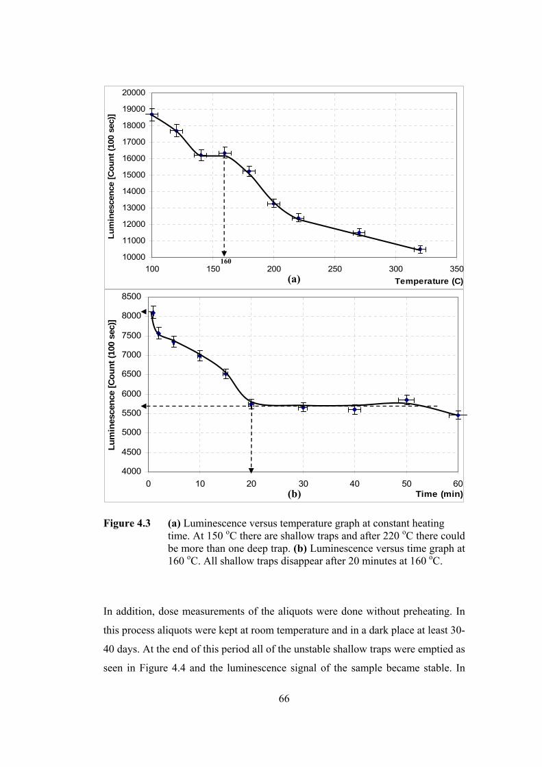
Figure 4.3 (a) Luminescence versus temperature graph at constant heating time. At 150 oC there are shallow traps and after 220 oC there could be more than one deep trap. (b) Luminescence versus time graph at 160 oC. All shallow traps disappear after 20 minutes at 160 oC.

In addition, dose measurements of the aliquots were done without preheating. In

this process aliquots were kept at room temperature and in a dark place at least 30-

40 days. At the end of this period all of the unstable shallow traps were emptied as

seen in Figure 4.4 and the luminescence signal of the sample became stable. In

4000

4500

5000

5500

6000

6500

7000

7500

8000

8500

0 10 20 30 40 50 6Time (min)

0

C0

Lum

ines

cenc

e [

ount

(10

sec

)]

10000

11000

12000

13000

14000

15000

16000

17000

18000

19000

20000

100 150 200 250 300 350Temperature (C)

ue

Lm

insc

ence

[Cou

nt (1

00 s

ec)]

160

(a)

(b)

66

this study, groups of aliquots were prepared from un-irradiated ceramic samples.

The 120 Gy dose was given to each aliquot and the aliquots were kept in a dark

place. The luminescences of each group of aliquots were measured and their doses

or dose rates were recorded.

In Figure 4.3b, the OSL intensity ratio of 5700 to 8200 is approximately 0.7.

Similarly, in Figure 4.4, the OSL intensity ratio of the 17000 to 25000 is again

approximately 0.7 as found in Figure 4.3b. This means, dose rate of the shallow

traps is approximately 30-35% of the total dose before preheating applied on the

polimineral sample aliquots.

0

5000

10000

15000

20000

25000

30000

0 10 20 30 40 50Day

Figure 4.4 Luminescence versus day graph for un-preheated polimineral aliquots. The fading of shallow traps ceases approximately after 40 days after irradiation.

Lum

ines

cenc

e s

[Cou

nt (1

00ec

)]

Fading of shallow traps at room temperature for un-preheated aliquots.

67

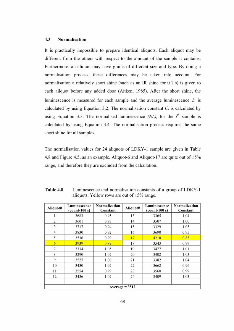
4.3 Normalisation

It is practically impossible to prepare identical aliquots. Each aliquot may be

different from the others with respect to the amount of the sample it contains.

Furthermore, an aliquot may have grains of different size and type. By doing a

normalisation process, these differences may be taken into account. For

normalisation a relatively short shine (such as an IR shine for 0.1 s) is given to

each aliquot before any added dose (Aitken, 1985). After the short shine, the

luminescence is measured for each sample and the average luminescence L is

calculated by using Equation 3.2. The normalisation constant Ci is calculated by

using Equation 3.3. The normalised luminescence (NL)i for the ith sample is

calculated by using Equation 3.4. The normalisation process requires the same

short shine for all samples.

The normalisation values for 24 aliquots of LDKY-1 sample are given in Table

4.8 and Figure 4.5, as an example. Aliquot-6 and Aliquot-17 are quite out of ±5%

range, and therefore they are excluded from the calculation.

Table 4.8 Luminescence and normalisation constants of a group of LDKY-1 aliquots. Yellow rows are out of ±5% range.

Aliquot# Luminescence (count-100 s)

Normalization Constant Aliquot# Luminescence

(count-100 s) Normalization

Constant 1 3683 0.95 13 3365 1.04 2 3601 0.97 14 3507 1.00 3 3717 0.94 15 3329 1.05 4 3830 0.92 16 3690 0.95 5 3536 0.99 17 4210 0.83 6 3939 0.89 18 3543 0.99 7 3334 1.05 19 3477 1.01 8 3290 1.07 20 3402 1.03 9 3527 1.00 21 3382 1.04

10 3430 1.02 22 3662 0.96 11 3554 0.99 23 3560 0.99 12 3436 1.02 24 3409 1.03

Average = 3512

68

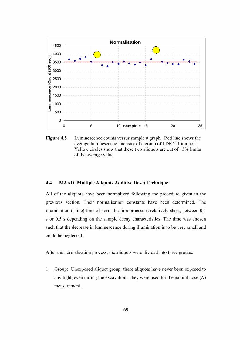
Normalisation

0

500

1000

1500

2000

2500

3000

3500

4000

4500

0 5 10 15 20 25Sample #

isc

ence

[Cou

nt (

neLu

m

100

sec)

]

Figure 4.5 Luminescence counts versus sample # graph. Red line shows the average luminescence intensity of a group of LDKY-1 aliquots. Yellow circles show that these two aliquots are out of ±5% limits of the average value.

4.4 MAAD (Multiple Aliquots Additive Dose) Technique

All of the aliquots have been normalized following the procedure given in the

previous section. Their normalisation constants have been determined. The

illumination (shine) time of normalisation process is relatively short, between 0.1

s or 0.5 s depending on the sample decay characteristics. The time was chosen

such that the decrease in luminescence during illumination is to be very small and

could be neglected.

After the normalisation process, the aliquots were divided into three groups:

1. Group: Unexposed aliquot group: these aliquots have never been exposed to

any light, even during the excavation. They were used for the natural dose (N)

measurement.

69

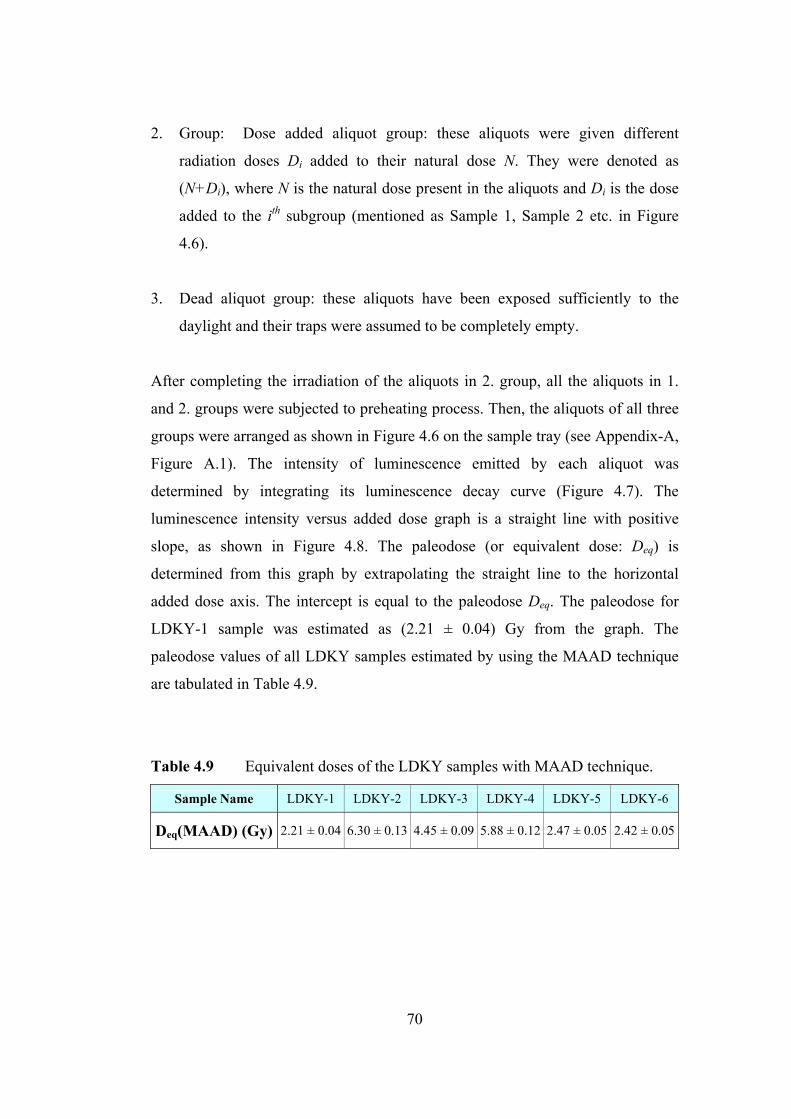
2. Group: Dose added aliquot group: these aliquots were given different

radiation doses Di added to their natural dose N. They were denoted as

(N+Di), where N is the natural dose present in the aliquots and Di is the dose

added to the ith subgroup (mentioned as Sample 1, Sample 2 etc. in Figure

4.6).

3. Dead aliquot group: these aliquots have been exposed sufficiently to the

daylight and their traps were assumed to be completely empty.

After completing the irradiation of the aliquots in 2. group, all the aliquots in 1.

and 2. groups were subjected to preheating process. Then, the aliquots of all three

groups were arranged as shown in Figure 4.6 on the sample tray (see Appendix-A,

Figure A.1). The intensity of luminescence emitted by each aliquot was

determined by integrating its luminescence decay curve (Figure 4.7). The

luminescence intensity versus added dose graph is a straight line with positive

slope, as shown in Figure 4.8. The paleodose (or equivalent dose: Deq) is

determined from this graph by extrapolating the straight line to the horizontal

added dose axis. The intercept is equal to the paleodose Deq. The paleodose for

LDKY-1 sample was estimated as (2.21 ± 0.04) Gy from the graph. The

paleodose values of all LDKY samples estimated by using the MAAD technique

are tabulated in Table 4.9.

Table 4.9 Equivalent doses of the LDKY samples with MAAD technique.

Sample Name LDKY-1 LDKY-2 LDKY-3 LDKY-4 LDKY-5 LDKY-6

Deq(MAAD) (Gy) 2.21 ± 0.04 6.30 ± 0.13 4.45 ± 0.09 5.88 ± 0.12 2.47 ± 0.05 2.42 ± 0.05

70

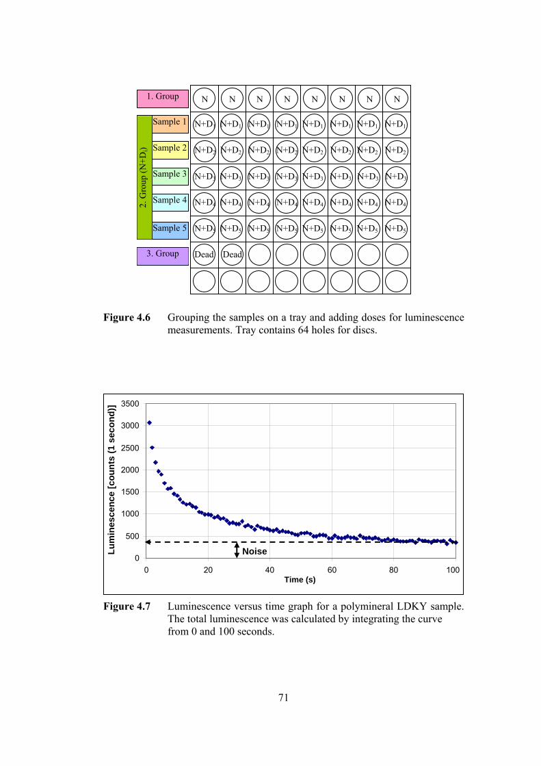
N+D1 N+D1 N+D1 N+D1 N+D1 N+D1 N+D1 N+D1

N+D2 N+D2 N+D2 N+D2 N+D2 N+D2 N+D2 N+D2

N+D3 N+D3 N+D3 N+D3 N+D3 N+D3 N+D3 N+D3

N+D4 N+D4 N+D4 N+D4 N+D4 N+D4 N+D4 N+D4

N+D5 N+D5 N+D5 N+D5 N+D5 N+D5 N+D5 N+D5

Dead Dead

N N N N N N N N 1. Group

Sample 2

Sample 3

Sample 4

Sample 5

Sample 1

3. Group

2. G

roup

(N+D

i)

Figure 4.6 Grouping the samples on a tray and adding doses for luminescence measurements. Tray contains 64 holes for discs.

Noise 0

500

1000

1500

2000

2500

3000

3500

0 20 40 60 80 100Time (s)

Lum

ine

Figure 4.7 Luminescence versus time graph for a polymineral LDKY sample. The total luminescence was calculated by integrating the curve from 0 and 100 seconds.

scen

ce [c

ount

s (1

sec

on)]d

Noise

71

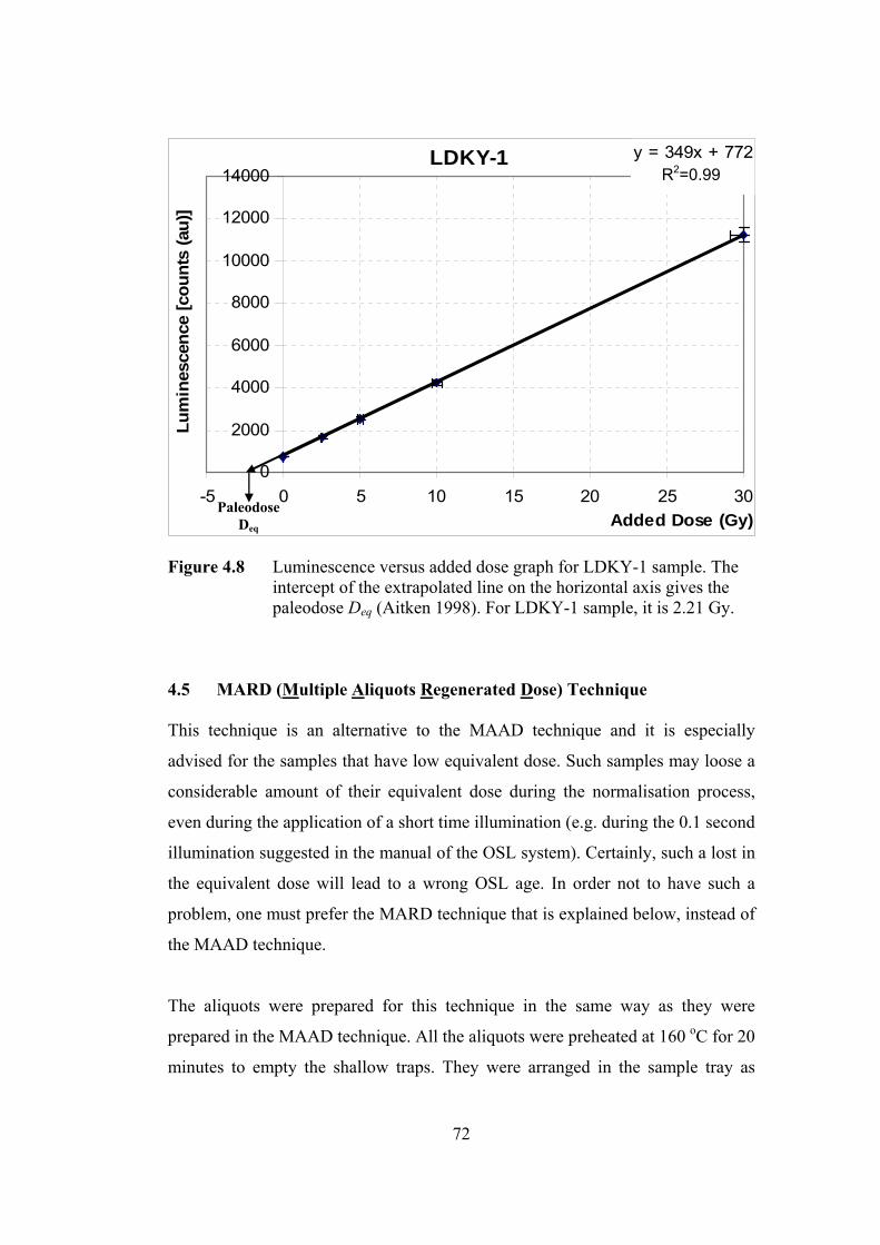
LDKY-1 y = 349x + 772R2 = 1

0

2000

4000

6000

8000

10000

12000

14000

-5 0 5 10 15 20 25 30Added Dose (Gy)

L

Figure 4.8 Luminescence versus added dose graph for LDKY-1 sample. The intercept of the extrapolated line on the horizontal axis gives the paleodose Deq (Aitken 1998). For LDKY-1 sample, it is 2.21 Gy.

4.5 MARD (Multiple Aliquots Regenerated Dose) Technique

This technique is an alternative to the MAAD technique and it is especially

advised for the samples that have low equivalent dose. Such samples may loose a

considerable amount of their equivalent dose during the normalisation process,

even during the application of a short time illumination (e.g. during the 0.1 second

illumination suggested in the manual of the OSL system). Certainly, such a lost in

the equivalent dose will lead to a wrong OSL age. In order not to have such a

problem, one must prefer the MARD technique that is explained below, instead of

the MAAD technique.

The aliquots were prepared for this technique in the same way as they were

prepared in the MAAD technique. All the aliquots were preheated at 160 oC for 20

minutes to empty the shallow traps. They were arranged in the sample tray as

umi

]ne

scen

ce [c

ount

s (a

u)R2=0.99

Paleodose Deq

72

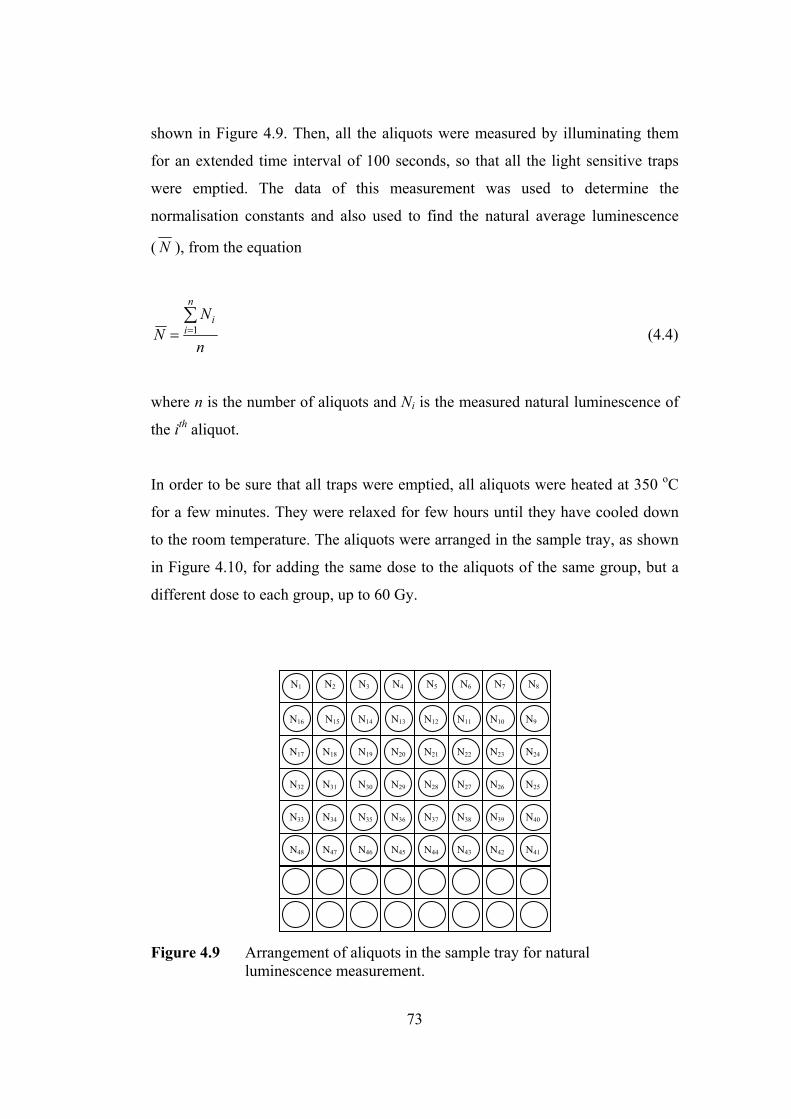
shown in Figure 4.9. Then, all the aliquots were measured by illuminating them

for an extended time interval of 100 seconds, so that all the light sensitive traps

were emptied. The data of this measurement was used to determine the

normalisation constants and also used to find the natural average luminescence

( N ), from the equation

n

NN

n

ii∑

== 1 (4.4)

where n is the number of aliquots and Ni is the measured natural luminescence of

the ith aliquot.

In order to be sure that all traps were emptied, all aliquots were heated at 350 oC

for a few minutes. They were relaxed for few hours until they have cooled down

to the room temperature. The aliquots were arranged in the sample tray, as shown

in Figure 4.10, for adding the same dose to the aliquots of the same group, but a

different dose to each group, up to 60 Gy.

N17 N18 N19 N20 N21 N22 N23 N24

N32 N31 N30 N29 N28 N27 N26 N25

N1 N2 N3 N4 N5 N6

N16 N15 N14 N13 N12 N11 N10 N9

N7 N8

N33 N34 N35 N36 N37 N38 N39 N40

N48 N47 N46 N45 N44 N43 N42 N41

Figure 4.9 Arrangement of aliquots in the sample tray for natural luminescence measurement.

73

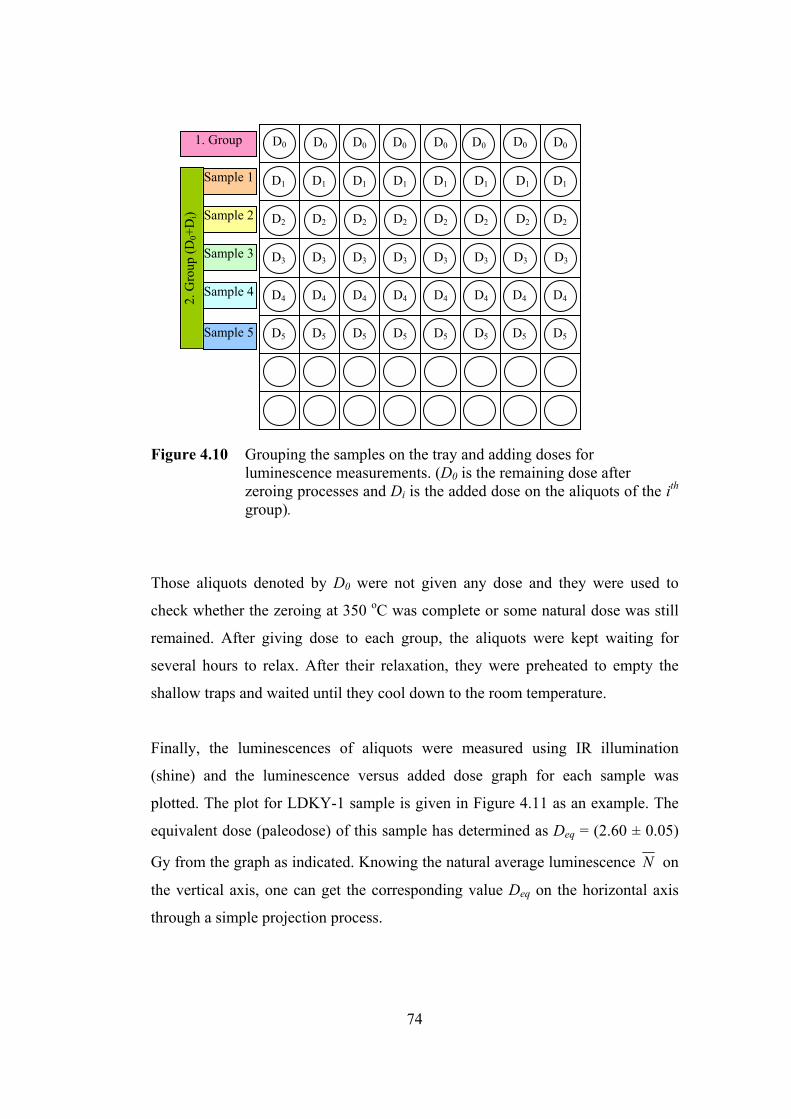
D1 D1 D1 D1 D1 D1 D1 D1

D2 D2 D2 D2 D2 D2 D2 D2

D3 D3 D3 D3 D3 D3 D3 D3

D4 D4 D4 D4 D4 D4 D4 D4

D5 D5 D5 D5 D5 D5 D5 D5

D0 1. Group

Sample 2

Sample 3

Sample 4

Sample 5

Sample 1 2.

Gro

up (D

0+D

i)

D0 D0 D0 D0 D0 D0 D0

Figure 4.10 Grouping the samples on the tray and adding doses for luminescence measurements. (D0 is the remaining dose after zeroing processes and Di is the added dose on the aliquots of the ith group).

Those aliquots denoted by D0 were not given any dose and they were used to

check whether the zeroing at 350 oC was complete or some natural dose was still

remained. After giving dose to each group, the aliquots were kept waiting for

several hours to relax. After their relaxation, they were preheated to empty the

shallow traps and waited until they cool down to the room temperature.

Finally, the luminescences of aliquots were measured using IR illumination

(shine) and the luminescence versus added dose graph for each sample was

plotted. The plot for LDKY-1 sample is given in Figure 4.11 as an example. The

equivalent dose (paleodose) of this sample has determined as Deq = (2.60 ± 0.05)

Gy from the graph as indicated. Knowing the natural average luminescence N on

the vertical axis, one can get the corresponding value Deq on the horizontal axis

through a simple projection process.

74

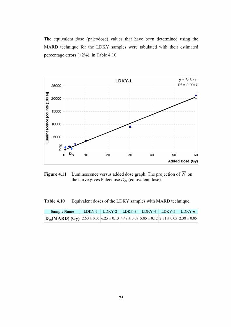
The equivalent dose (paleodose) values that have been determined using the

MARD technique for the LDKY samples were tabulated with their estimated

percentage errors (±2%), in Table 4.10.

LDKY-1 y = 346.4xR2 = 0.9917

0

5000

10000

15000

20000

25000

0 10 20 30 40 50 6

Added Dose (Gy)

ts (1

00 s

)]

Figure 4.11 Luminescence versus added dose graph. The projection of N on the curve gives Paleodose Deq (equivalent dose).

Table 4.10 Equivalent doses of the LDKY samples with MARD technique.

Sample Name LDKY-1 LDKY-2 LDKY-3 LDKY-4 LDKY-5 LDKY-6

Deq(MARD) (Gy) 2.60 ± 0.05 6.25 ± 0.13 4.48 ± 0.09 5.85 ± 0.12 2.51 ± 0.05 2.38 ± 0.05

0

Lum

ines

cenc

e [c

oun

NDeq

75

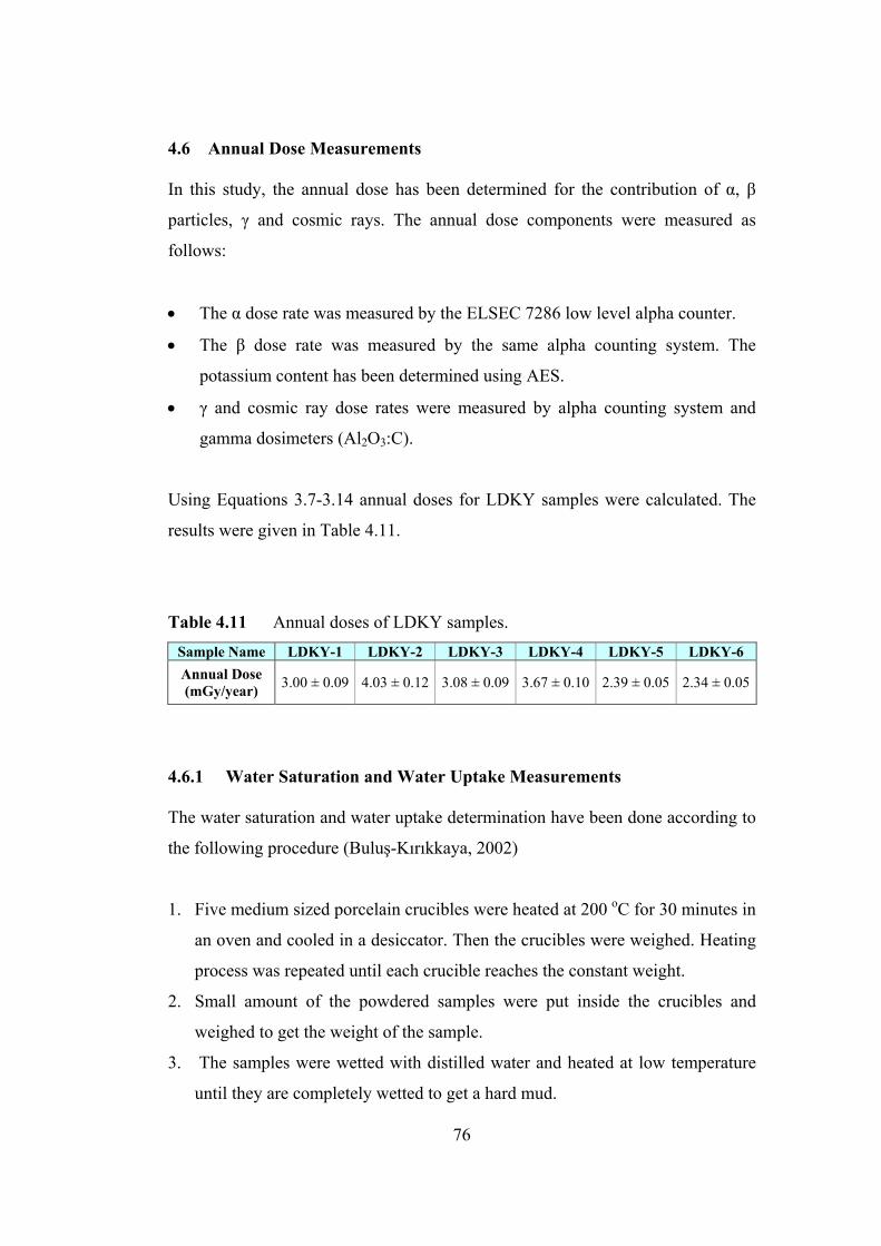
4.6 Annual Dose Measurements

In this study, the annual dose has been determined for the contribution of α, β

particles, γ and cosmic rays. The annual dose components were measured as

follows:

• The α dose rate was measured by the ELSEC 7286 low level alpha counter.

• The β dose rate was measured by the same alpha counting system. The

potassium content has been determined using AES.

• γ and cosmic ray dose rates were measured by alpha counting system and

gamma dosimeters (Al2O3:C).

Using Equations 3.7-3.14 annual doses for LDKY samples were calculated. The

results were given in Table 4.11.

Table 4.11 Annual doses of LDKY samples. Sample Name LDKY-1 LDKY-2 LDKY-3 LDKY-4 LDKY-5 LDKY-6 Annual Dose (mGy/year) 3.00 ± 0.09 4.03 ± 0.12 3.08 ± 0.09 3.67 ± 0.10 2.39 ± 0.05 2.34 ± 0.05

4.6.1 Water Saturation and Water Uptake Measurements

The water saturation and water uptake determination have been done according to

the following procedure (Buluş-Kırıkkaya, 2002)

1. Five medium sized porcelain crucibles were heated at 200 oC for 30 minutes in

an oven and cooled in a desiccator. Then the crucibles were weighed. Heating

process was repeated until each crucible reaches the constant weight.

2. Small amount of the powdered samples were put inside the crucibles and

weighed to get the weight of the sample.

3. The samples were wetted with distilled water and heated at low temperature

until they are completely wetted to get a hard mud.

76

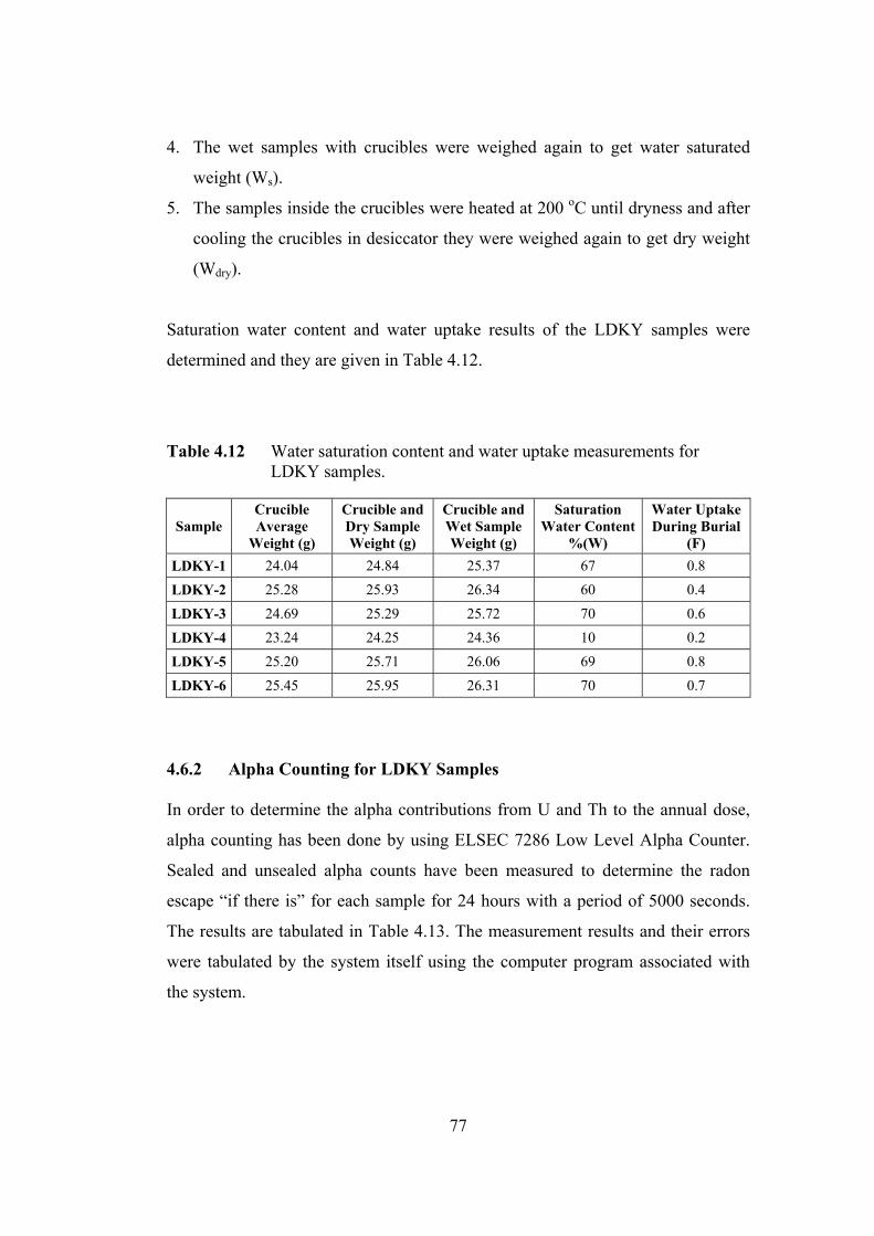
4. The wet samples with crucibles were weighed again to get water saturated

weight (Ws).

5. The samples inside the crucibles were heated at 200 oC until dryness and after

cooling the crucibles in desiccator they were weighed again to get dry weight

(Wdry).

Saturation water content and water uptake results of the LDKY samples were

determined and they are given in Table 4.12.

Table 4.12 Water saturation content and water uptake measurements for LDKY samples.

Sample Crucible Average

Weight (g)

Crucible and Dry Sample Weight (g)

Crucible and Wet Sample Weight (g)

Saturation Water Content

%(W)

Water Uptake During Burial

(F) LDKY-1 24.04 24.84 25.37 67 0.8

LDKY-2 25.28 25.93 26.34 60 0.4

LDKY-3 24.69 25.29 25.72 70 0.6 LDKY-4 23.24 24.25 24.36 10 0.2

LDKY-5 25.20 25.71 26.06 69 0.8

LDKY-6 25.45 25.95 26.31 70 0.7

4.6.2 Alpha Counting for LDKY Samples

In order to determine the alpha contributions from U and Th to the annual dose,

alpha counting has been done by using ELSEC 7286 Low Level Alpha Counter.

Sealed and unsealed alpha counts have been measured to determine the radon

escape “if there is” for each sample for 24 hours with a period of 5000 seconds.

The results are tabulated in Table 4.13. The measurement results and their errors

were tabulated by the system itself using the computer program associated with

the system.

77

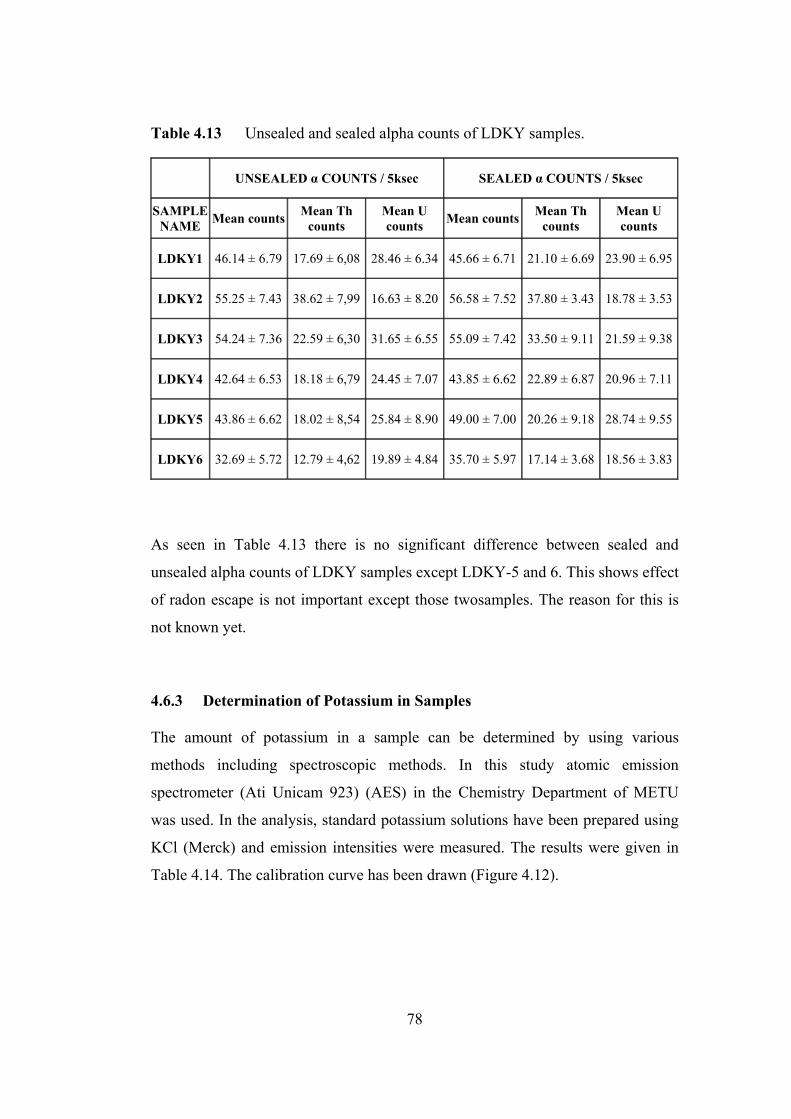
Table 4.13 Unsealed and sealed alpha counts of LDKY samples.

UNSEALED α COUNTS / 5ksec SEALED α COUNTS / 5ksec

SAMPLE NAME Mean counts Mean Th

counts Mean U counts Mean counts Mean Th

counts Mean U counts

LDKY1 46.14 ± 6.79 17.69 ± 6,08 28.46 ± 6.34 45.66 ± 6.71 21.10 ± 6.69 23.90 ± 6.95

LDKY2 55.25 ± 7.43 38.62 ± 7,99 16.63 ± 8.20 56.58 ± 7.52 37.80 ± 3.43 18.78 ± 3.53

LDKY3 54.24 ± 7.36 22.59 ± 6,30 31.65 ± 6.55 55.09 ± 7.42 33.50 ± 9.11 21.59 ± 9.38

LDKY4 42.64 ± 6.53 18.18 ± 6,79 24.45 ± 7.07 43.85 ± 6.62 22.89 ± 6.87 20.96 ± 7.11

LDKY5 43.86 ± 6.62 18.02 ± 8,54 25.84 ± 8.90 49.00 ± 7.00 20.26 ± 9.18 28.74 ± 9.55

LDKY6 32.69 ± 5.72 12.79 ± 4,62 19.89 ± 4.84 35.70 ± 5.97 17.14 ± 3.68 18.56 ± 3.83

As seen in Table 4.13 there is no significant difference between sealed and

unsealed alpha counts of LDKY samples except LDKY-5 and 6. This shows effect

of radon escape is not important except those twosamples. The reason for this is

not known yet.

4.6.3 Determination of Potassium in Samples

The amount of potassium in a sample can be determined by using various

methods including spectroscopic methods. In this study atomic emission

spectrometer (Ati Unicam 923) (AES) in the Chemistry Department of METU

was used. In the analysis, standard potassium solutions have been prepared using

KCl (Merck) and emission intensities were measured. The results were given in

Table 4.14. The calibration curve has been drawn (Figure 4.12).

78

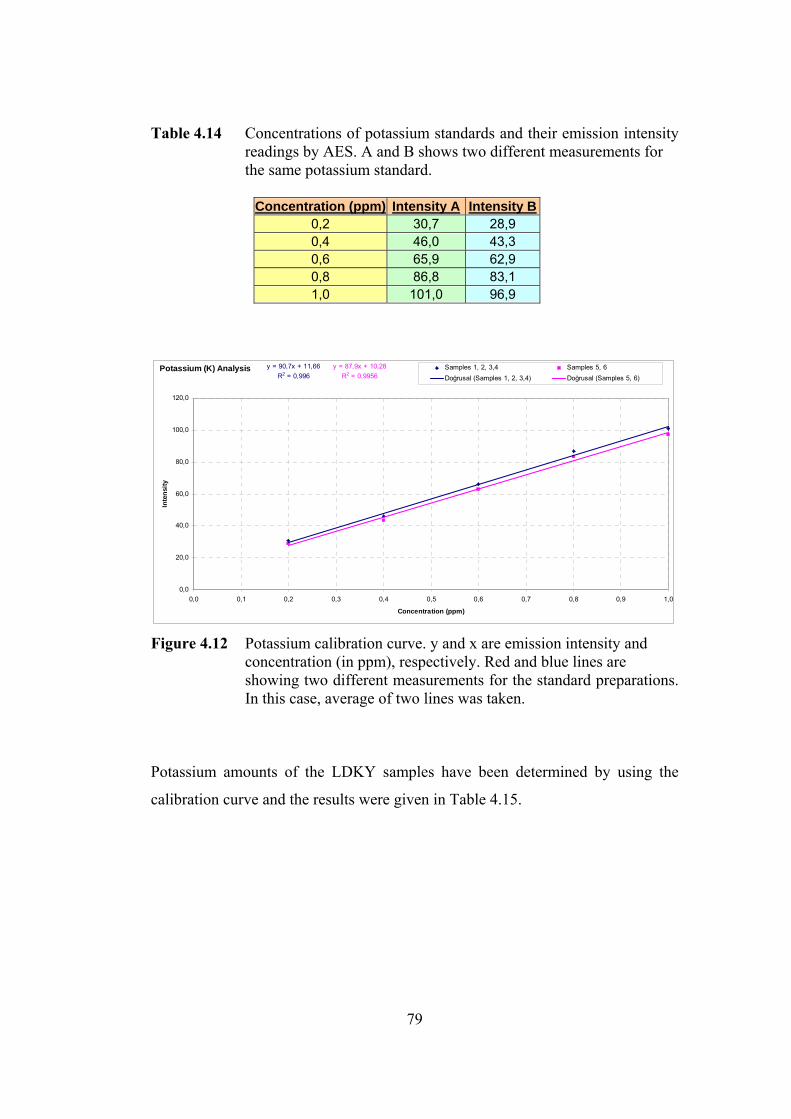
Table 4.14 Concentrations of potassium standards and their emission intensity readings by AES. A and B shows two different measurements for the same potassium standard.

Concentration (ppm) Intensity A Intensity B0,2 30,7 28,9 0,4 46,0 43,3 0,6 65,9 62,9 0,8 86,8 83,1 1,0 101,0 96,9

Potassium (K) Analysis y = 90,7x + 11,66

R2 = 0,996y = 87,9x + 10,28

R2 = 0,9956

0,0

20,0

40,0

60,0

80,0

100,0

120,0

0,0 0,1 0,2 0,3 0,4 0,5 0,6 0,7 0,8 0,9 1,0

Concentration (ppm)

Inte

nsity

Samples 1, 2, 3,4 Samples 5, 6Doğrusal (Samples 1, 2, 3,4) Doğrusal (Samples 5, 6)

Figure 4.12 Potassium calibration curve. y and x are emission intensity and concentration (in ppm), respectively. Red and blue lines are showing two different measurements for the standard preparations. In this case, average of two lines was taken.

Potassium amounts of the LDKY samples have been determined by using the

calibration curve and the results were given in Table 4.15.

79

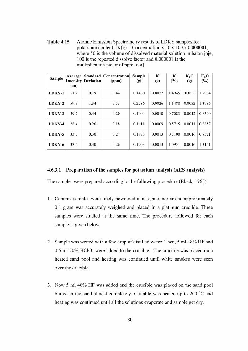
Table 4.15 Atomic Emission Spectrometry results of LDKY samples for potassium content. [K(g) = Concentration x 50 x 100 x 0.000001, where 50 is the volume of dissolved material solution in balon joje, 100 is the repeated dissolve factor and 0.000001 is the multiplication factor of ppm to g]

Sample

Average Intensity

(au)

Standard Deviation

Concentration (ppm)

Sample (g)

K (g)

K (%)

K2O (g)

K2O (%)

LDKY-1 51.2 0.19 0.44 0.1460 0.0022 1.4945 0.026 1.7934

LDKY-2 59.3 1.34 0.53 0.2286 0.0026 1.1488 0.0032 1.3786

LDKY-3 29.7 0.44 0.20 0.1404 0.0010 0.7083 0.0012 0.8500

LDKY-4 28.4 0.26 0.18 0.1611 0.0009 0.5715 0.0011 0.6857

LDKY-5 33.7 0.30 0.27 0.1873 0.0013 0.7100 0.0016 0.8521

LDKY-6 33.4 0.30 0.26 0.1203 0.0013 1.0951 0.0016 1.3141

4.6.3.1 Preparation of the samples for potassium analysis (AES analysis)

The samples were prepared according to the following procedure (Black, 1965):

1. Ceramic samples were finely powdered in an agate mortar and approximately

0.1 gram was accurately weighed and placed in a platinum crucible. Three

samples were studied at the same time. The procedure followed for each

sample is given below.

2. Sample was wetted with a few drop of distilled water. Then, 5 ml 48% HF and

0.5 ml 70% HClO4 were added to the crucible. The crucible was placed on a

heated sand pool and heating was continued until white smokes were seen

over the crucible.

3. Now 5 ml 48% HF was added and the crucible was placed on the sand pool

buried in the sand almost completely. Crucible was heated up to 200 oC and

heating was continued until all the solutions evaporate and sample get dry.

80

4. After the crucible was cool down, 2 ml distilled water and a few drop of

HClO4 were added. The crucible was placed inside the sand pool and heating

was continued until all the liquid evaporates.

5. After cooling the crucible, 5ml of 6M HCl and 5 ml distilled water were

added. This time crucible was heated with Bunsen burner until the solution

was boiled and the sample was dried. Here, sample was expected to be fused

completely.

6. If considerable amount of sample remained, fusion process (step 1 to 5)

should be repeated.

7. The fused sample was treated with dilute HCl. Then, filtered using blue band

filter paper. The filtrate was put in 50 ml or 100 ml graduated flask and diluted

to the mark with distilled water.

4.6.4 Contribution of Gamma and Cosmic rays for Dose Rate

To determine the gamma (γ) and cosmic ray components of the annual dose, the

thick Al2O3:C Thermo-Luminescence Dosimeters (TLD) were used. These

dosimeters are very sensitive to any kind of radiation, including the cosmic rays.

In this work eight commercial thick TLD were used. They were heated at 400 oC

(Buluş-Kırıkkaya, 2002) to empty all the traps completely. In order to determine

the gamma dose response characteristics of the dosimeters, they were exposed to γ

radiation in “Ankara Nükleer Araştırma ve Eğitim Merkezi” and their TL were

measured with the “Harshaw TL system” in the same laboratory. The

measurement results are tabulated in Table 4.16 and the gamma dose response

curve is given in Figure 4.13. The system used has recorded the amount of TL

accumulated as TL voltage and therefore a TL voltage versus dose graph was

plotted.

81

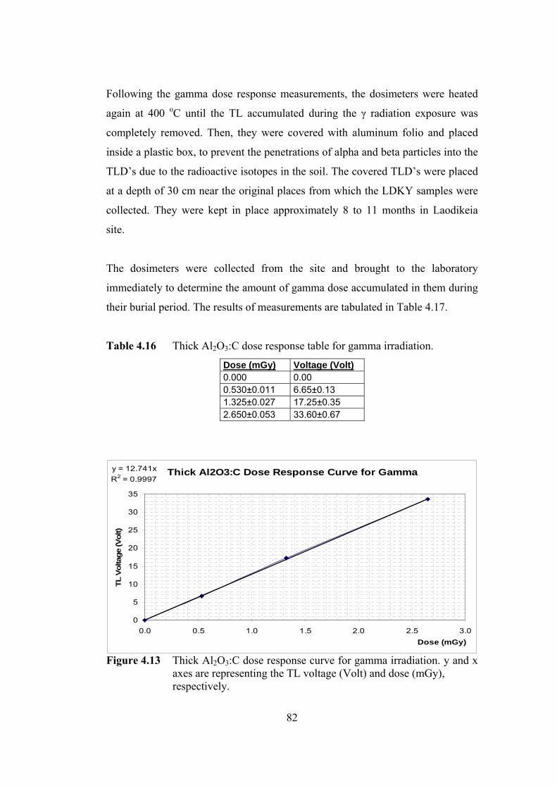
Following the gamma dose response measurements, the dosimeters were heated

again at 400 oC until the TL accumulated during the γ radiation exposure was

completely removed. Then, they were covered with aluminum folio and placed

inside a plastic box, to prevent the penetrations of alpha and beta particles into the

TLD’s due to the radioactive isotopes in the soil. The covered TLD’s were placed

at a depth of 30 cm near the original places from which the LDKY samples were

collected. They were kept in place approximately 8 to 11 months in Laodikeia

site.

The dosimeters were collected from the site and brought to the laboratory

immediately to determine the amount of gamma dose accumulated in them during

their burial period. The results of measurements are tabulated in Table 4.17.

Table 4.16 Thick Al2O3:C dose response table for gamma irradiation.

Dose (mGy) Voltage (Volt)0.000 0.00 0.530±0.011 6.65±0.13 1.325±0.027 17.25±0.35 2.650±0.053 33.60±0.67

Thick Al2O3:C Dose Response Curve for Gammay = 12.741xR2 = 0.9997

0

5

10

15

20

25

30

35

0.0 0.5 1.0 1.5 2.0 2.5 3.0Dose (mGy)

TL V

olta

ge (V

olt)

Figure 4.13 Thick Al2O3:C dose response curve for gamma irradiation. y and x axes are representing the TL voltage (Volt) and dose (mGy), respectively.

82

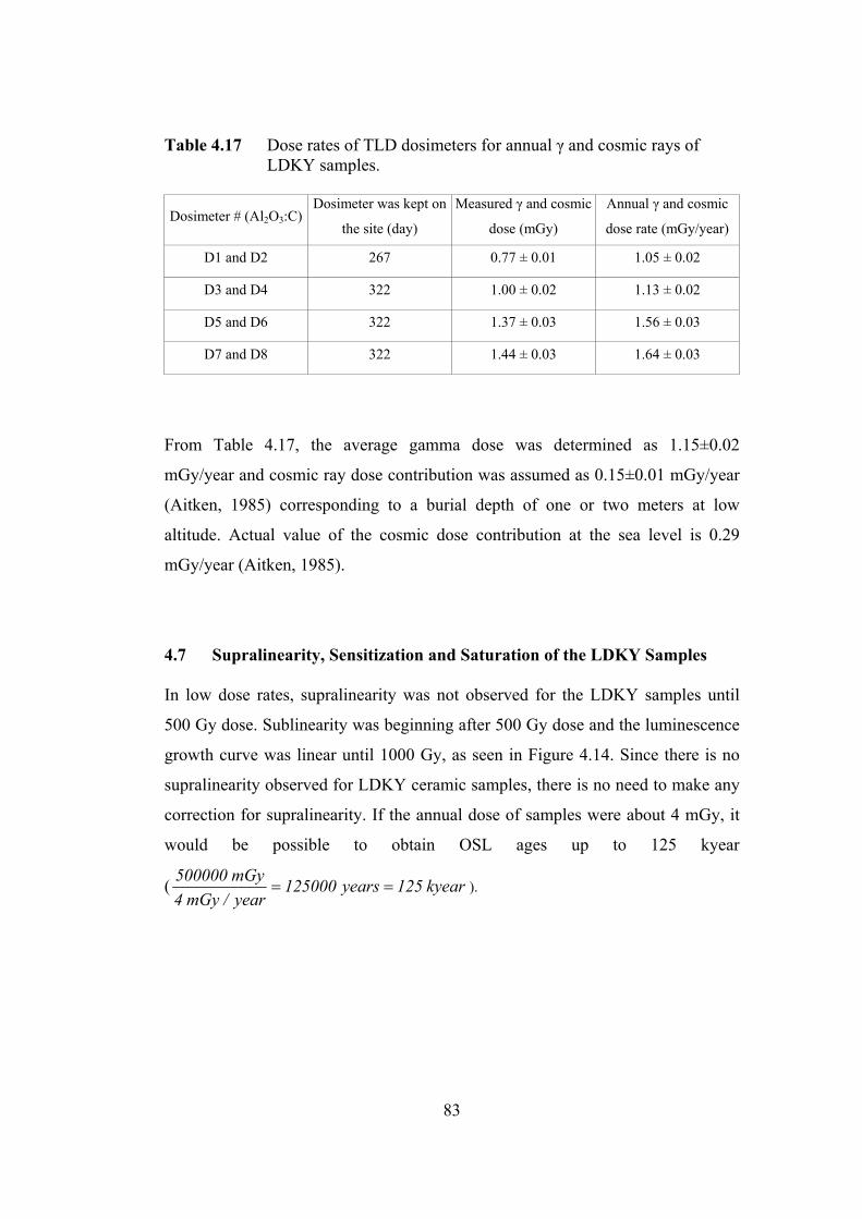
Table 4.17 Dose rates of TLD dosimeters for annual γ and cosmic rays of LDKY samples.

Dosimeter # (Al2O3:C) Dosimeter was kept on

the site (day)

Measured γ and cosmic

dose (mGy)

Annual γ and cosmic

dose rate (mGy/year)

D1 and D2 267 0.77 ± 0.01 1.05 ± 0.02

D3 and D4 322 1.00 ± 0.02 1.13 ± 0.02

D5 and D6 322 1.37 ± 0.03 1.56 ± 0.03

D7 and D8 322 1.44 ± 0.03 1.64 ± 0.03

From Table 4.17, the average gamma dose was determined as 1.15±0.02

mGy/year and cosmic ray dose contribution was assumed as 0.15±0.01 mGy/year

(Aitken, 1985) corresponding to a burial depth of one or two meters at low

altitude. Actual value of the cosmic dose contribution at the sea level is 0.29

mGy/year (Aitken, 1985).

4.7 Supralinearity, Sensitization and Saturation of the LDKY Samples

In low dose rates, supralinearity was not observed for the LDKY samples until

500 Gy dose. Sublinearity was beginning after 500 Gy dose and the luminescence

growth curve was linear until 1000 Gy, as seen in Figure 4.14. Since there is no

supralinearity observed for LDKY ceramic samples, there is no need to make any

correction for supralinearity. If the annual dose of samples were about 4 mGy, it

would be possible to obtain OSL ages up to 125 kyear

( kyear 125years 125000year/mGy 4mGy 500000

== ).

83

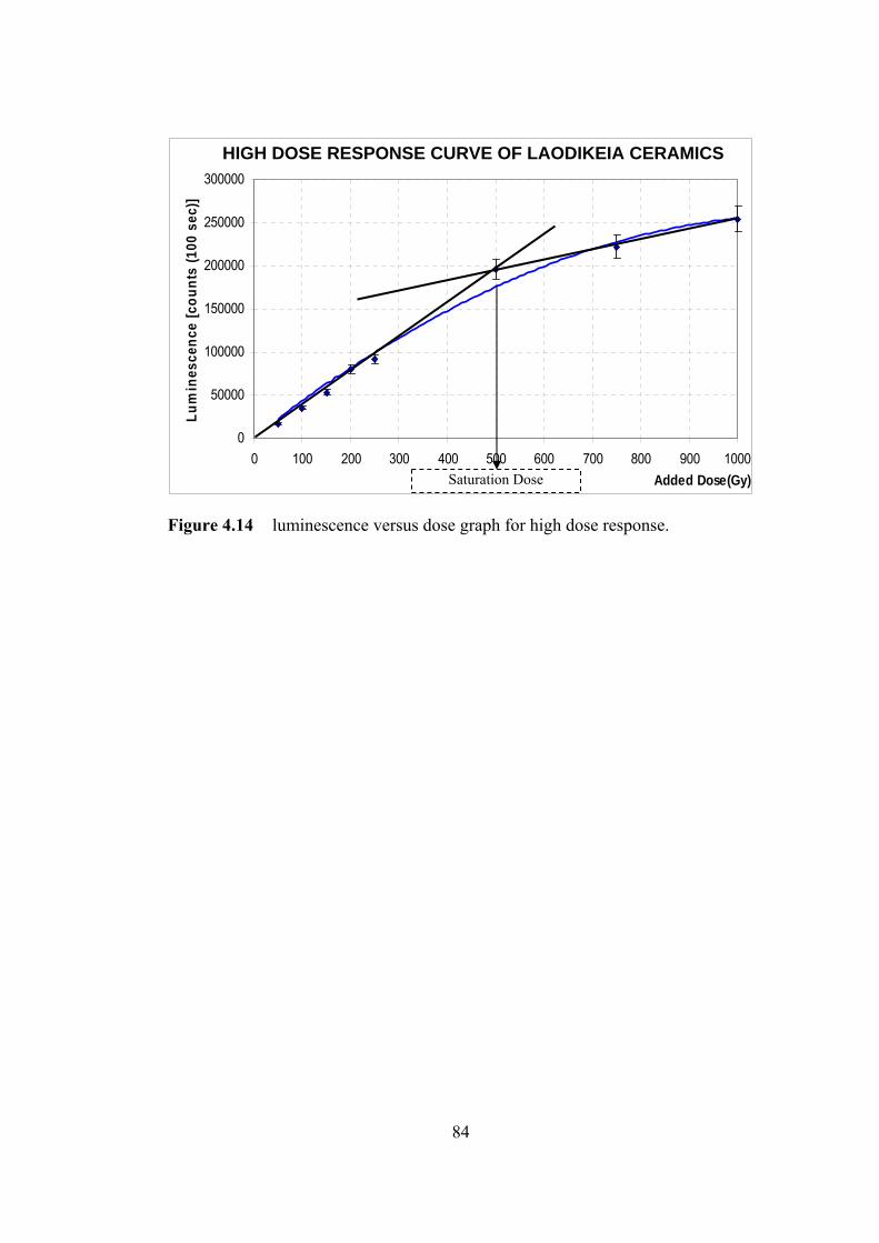
HIGH DOSE RESPONSE OF LAODIKEIA CERAMICS

0

50000

100000

150000

200000

250000

300000

0 100 200 300 400 500 600 700 800 900 1000Added Dose(Gy)

Lum

ines

cenc

e [c

ount

s (1

00 s

ec)]

Saturation Dose

HIGH DOSE RESPONSE CURVE OF LAODIKEIA CERAMICS

Figure 4.14 luminescence versus dose graph for high dose response.

84

CHAPTER 5

CONCLUSIONS

In this work, the optically stimulated luminescence of the ceramic samples

collected from Laodikeia archaeological site was measured with ELSEC 9010

optical dating system. An array of IR diode was used to stimulate only the

feldspar component of the samples. The data obtained was normalized using the

normalization technique (Aitken, 1985). Equivalent dose (Deq) was determined by

the additive dose technique, in which the laboratory doses were added to the

aliquots of the natural sample and the growth curve is extrapolated to zero

luminescence signal to obtain the equivalent dose values. Samples were irradiated

by a Sr-90 β source which has 0.0269 Gy/s dose rate for feldspar.

All the shallow electron traps that were filled during the laboratory irradiation

were emptied by applying preheating process at 160 oC for 20 minutes. Then, they

were illuminated by the IR light to measure the luminescence.

The uranium and thorium contribution to annual dose rate were determined by

low level alpha counting (Elsec low level alpha counter 7286) system.

Contribution of potassium content have been determined by using the atomic

emission spectrometry (AES) and the cosmic ray component of annual dose rate

was determined by placing TLD discs (Al2O3:C) at the site where samples were

collected.

The ages calculated for the LDKY samples were found to be consistent with the

values expected by the archaeologists.

85

The results of the study are promising and need further study, especially for the

annual dose measurements. In this work, the age calculations were based on actual

measurement results, but also some assumptions were made. In the annual dose

calculation, suggested values of a, b and k parameters (Aitken, 1985) were used.

These parameters for the LDKY site can also be determined experimentally in the

future works.

There was no chronology done for LDKY site, based on laboratory techniques as

far as archaeologists stated. Therefore, to establish a chronology for the site based

on OSL technique has considerable importance.

In determining the annual dose of the samples, following assumptions were made;

• The LDKY samples had constant annual dose rate during their burial time.

• In the measurements, humidity of the sample was assumed to be zero,

although samples may contain some amount of humidity.

In determining the annual dose and equivalent dose of the samples, the following

precautions were taken;

• The samples were taken from the same level and they were close to each

other.

• The samples were kept open after grinding for radon escape.

• The samples always were stored up in a dark place.

• The samples were handled all the times in red light.

Annual dose has been calculated from internal radioactive impurities of the

sample itself such as U, Th and K. These elements emit α, β particles and γ

radiation. The dose rate contributions of α, β particles and γ radiation have been

determined with different methods. The α contribution has been determined by

using alpha counter which measures the total amount of alpha particles coming

from radioactive impurities (U and Th). The β and γ contributions have been

determined by using alpha counter and potassium amount using AES.

86

Radon escape has been observed by measuring the alpha particles with sealed and

unsealed fine grained samples. However, there was no appreciable difference

between sealed and unsealed α measurements. Therefore, it can be assumed that

radon escape has no effect in annual dose measurements.

Instead of applying preheating process to the radiated aliquots in order to remove

the electrons from shallow traps, a correction factor can be used as a constant for

polimineral fine grain aliquots. In this study, this correction factor has been found

as 0.7. Because, the 30% of the total Luminescence (counts) were disappeared

during the 20 minutes preheating at 160 oC. In addition, the fading of the un-

preheated aliquots occurs during the 30-40 days period at room temperature.

However, this work has been done three times for one ceramic sample (LDKY-3).

Therefore, it is difficult to say that the founded correction factor is exactly suitable

and same for all other types of the samples.

For the further studies, annual and equivalent doses of the samples must be

determined with some other techniques and methods by using alternative devices.

As a suggestion, for the annual dose determination U, Th and K amounts can be

determined altogether by using a method such as Inductively Coupled Plasma –

Optical Emission Spectroscopy (ICP-OES) or an X-Ray Fluorescence (XRF).

For the LDKY samples one can also use quartz component of the samples in the

OSL measurement.

As mentioned before, LDKY samples have not shown any supralinearity and

sensitivities were constant for all LDKY samples. Saturation started after 500 Gy

for LDKY ceramic samples and this shows that ceramic is a good natural

dosimeter and age estimation can be done up to 100-150 kyear without making

any supralinearity correction.

87

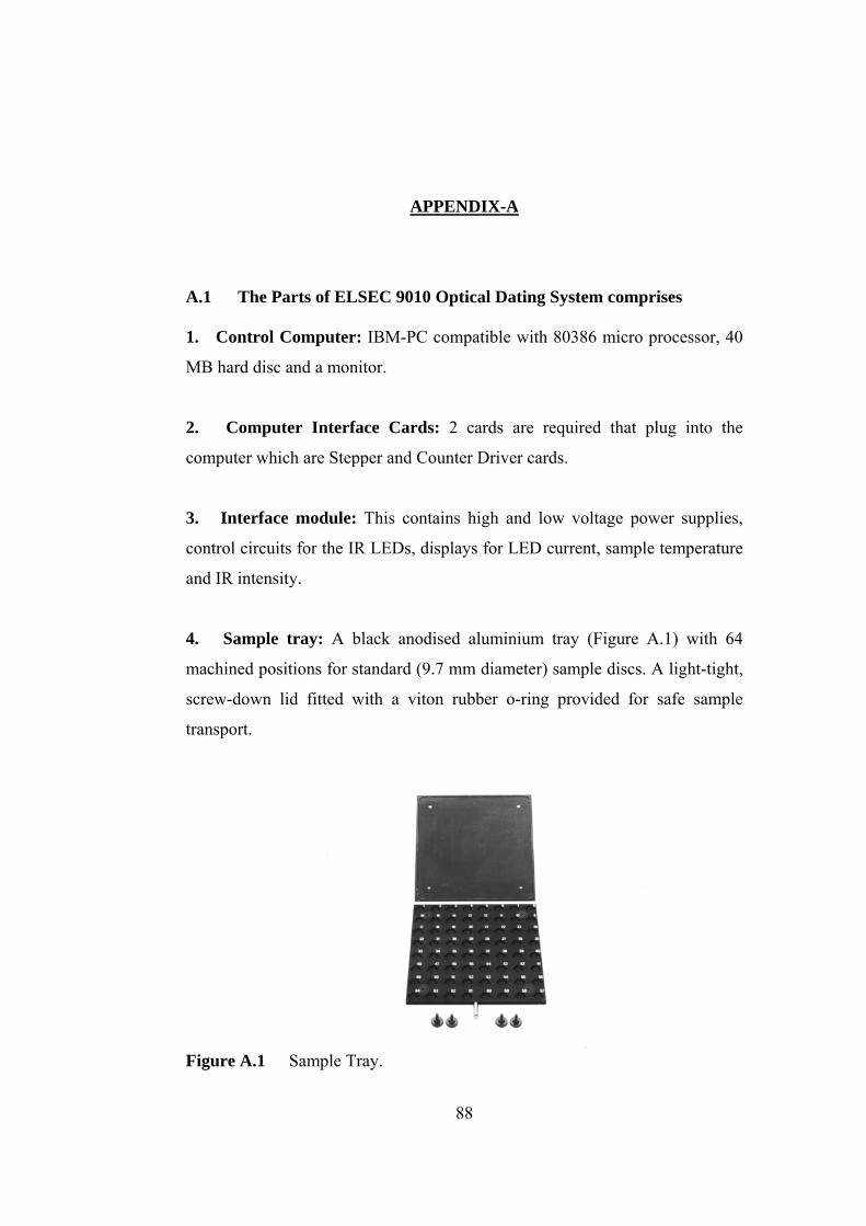
APPENDIX-A

A.1 The Parts of ELSEC 9010 Optical Dating System comprises

1. Control Computer: IBM-PC compatible with 80386 micro processor, 40

MB hard disc and a monitor.

2. Computer Interface Cards: 2 cards are required that plug into the

computer which are Stepper and Counter Driver cards.

3. Interface module: This contains high and low voltage power supplies,

control circuits for the IR LEDs, displays for LED current, sample temperature

and IR intensity.

4. Sample tray: A black anodised aluminium tray (Figure A.1) with 64

machined positions for standard (9.7 mm diameter) sample discs. A light-tight,

screw-down lid fitted with a viton rubber o-ring provided for safe sample

transport.

Figure A.1 Sample Tray.

88

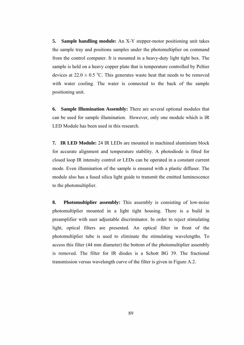
5. Sample handling module: An X-Y stepper-motor positioning unit takes

the sample tray and positions samples under the photomultiplier on command

from the control computer. It is mounted in a heavy-duty light tight box. The

sample is held on a heavy copper plate that is temperature controlled by Peltier

devices at 22.0 ± 0.5 oC. This generates waste heat that needs to be removed

with water cooling. The water is connected to the back of the sample

positioning unit.

6. Sample Illumination Assembly: There are several optional modules that

can be used for sample illumination. However, only one module which is IR

LED Module has been used in this research.

7. IR LED Module: 24 IR LEDs are mounted in machined aluminium block

for accurate alignment and temperature stability. A photodiode is fitted for

closed loop IR intensity control or LEDs can be operated in a constant current

mode. Even illumination of the sample is ensured with a plastic diffuser. The

module also has a fused silica light guide to transmit the emitted luminescence

to the photomultiplier.

8. Photomultiplier assembly: This assembly is consisting of low-noise

photomultiplier mounted in a light tight housing. There is a build in

preamplifier with user adjustable discriminator. In order to reject stimulating

light, optical filters are presented. An optical filter in front of the

photomultiplier tube is used to eliminate the stimulating wavelengths. To

access this filter (44 mm diameter) the bottom of the photomultiplier assembly

is removed. The filter for IR diodes is a Schott BG 39. The fractional

transmission versus wavelength curve of the filter is given in Figure A.2.

89

Frac

tiona

l Tra

nsm

issi

on

Wavelength - nm

Figure A.2 The graph of fractional transmission versus wavelength of Schott BG 39 filter. http://www.galvoptics.fsnet.co.uk/bg39.htm

9. Printer: It is an 80 column 24 pin dot matrix printer. It is used to print out

the data collected by the computer.

10. Software: The standard program supplied with OSL unit. “OSL” software

allows the user to manually control the unit, sample position under the

photomultiplier and record data on a sample by sample basis. Alternatively,

the system can be set up to automatically record the results for all 64 (or fewer)

samples on the tray. Results can be viewed and edited in tabular form. All

shine curves (i.e. the luminescence signal observed) can be viewed on screen

either singly, overlain as a group for a given dose point or the full data set can

be shown with color coding of each dose group. These graphs can be dumped

to a dot matrix printer, plotted on a pen plotter or laser printer or converted to

PCX format (PCX files are used for graphic data storage) for incorporation in

to word processed documents. Data are stored in binary format and full

information on file structure is provided to enable the user to write software to

access the results. Utilities are provided to convert results to ASCII (American

Standard Code for Information Interchange is a character encoding based on

the English alphabet) text can be read into spreadsheets.

90

11. “PLATO” software: This is the main data analysis program. “PLATO”

and the “OSL” programs are designed to be flexible and to permit different

methods of paleodose estimation. The period over which luminescence is

measured can be subdivided into a maximum 16383 channels with variable

duration (10 ms to 43x106 seconds with 10 ms resolution). This permits user

selection of the integration periods of interest, such as greater time resolution

of the shine curves in the early stages of the luminescence decay.

Normalization factors can be either read in from a pre-measured “short

exposure” file or inserted by the user. The background subtracted from each

shine curve can be chosen from the mean count rate of the final part of that

shine curve, a value obtained from a “dead” sample or a user inserted number.

A separate growth curve fitting for each integral period is currently performed

both by linear fitting and exponential fitting using an algorithm developed by

B.W. Smith (9010 Optical Dating System user Manual, 1993). Additional

curve fitting algorithms can be incorporated.

12. “AGE” software: This program takes the paleodose from the “PLATO”

program and other user input dosimetric data (such as radioisotope

concentrations or fractional dose rates, cosmic ray dose rate, water content,

burial depth etc.) and calculates an age for the sample and an error estimate for

that age.

13. Beta Irradiator unit: Sr-90 source was installed the system shown in

Figure A.3. The radioisotope compound is incorporated into the front surface

of the silver disc in a very thin layer about 2mm for a 1.5 GBq source. There is

a 0.1 mm screen of silver on which is a protective coating of gold or palladium.

91

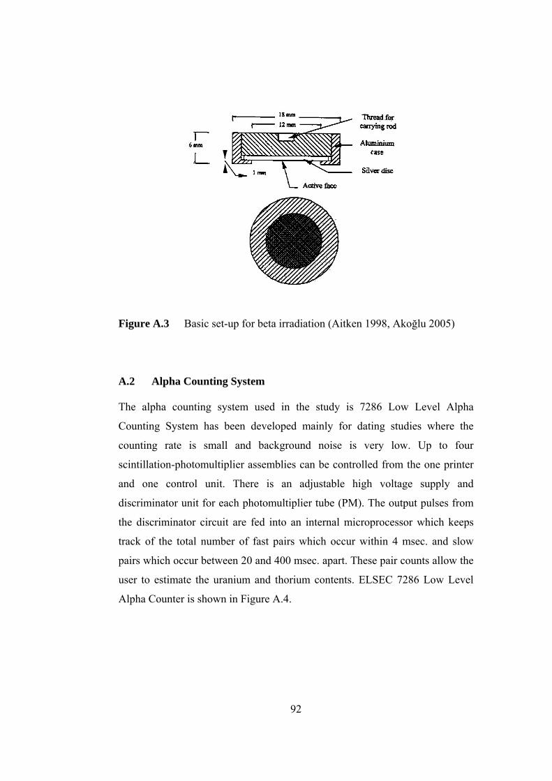
Figure A.3 Basic set-up for beta irradiation (Aitken 1998, Akoğlu 2005)

A.2 Alpha Counting System

The alpha counting system used in the study is 7286 Low Level Alpha

Counting System has been developed mainly for dating studies where the

counting rate is small and background noise is very low. Up to four

scintillation-photomultiplier assemblies can be controlled from the one printer

and one control unit. There is an adjustable high voltage supply and

discriminator unit for each photomultiplier tube (PM). The output pulses from

the discriminator circuit are fed into an internal microprocessor which keeps

track of the total number of fast pairs which occur within 4 msec. and slow

pairs which occur between 20 and 400 msec. apart. These pair counts allow the

user to estimate the uranium and thorium contents. ELSEC 7286 Low Level

Alpha Counter is shown in Figure A.4.

92

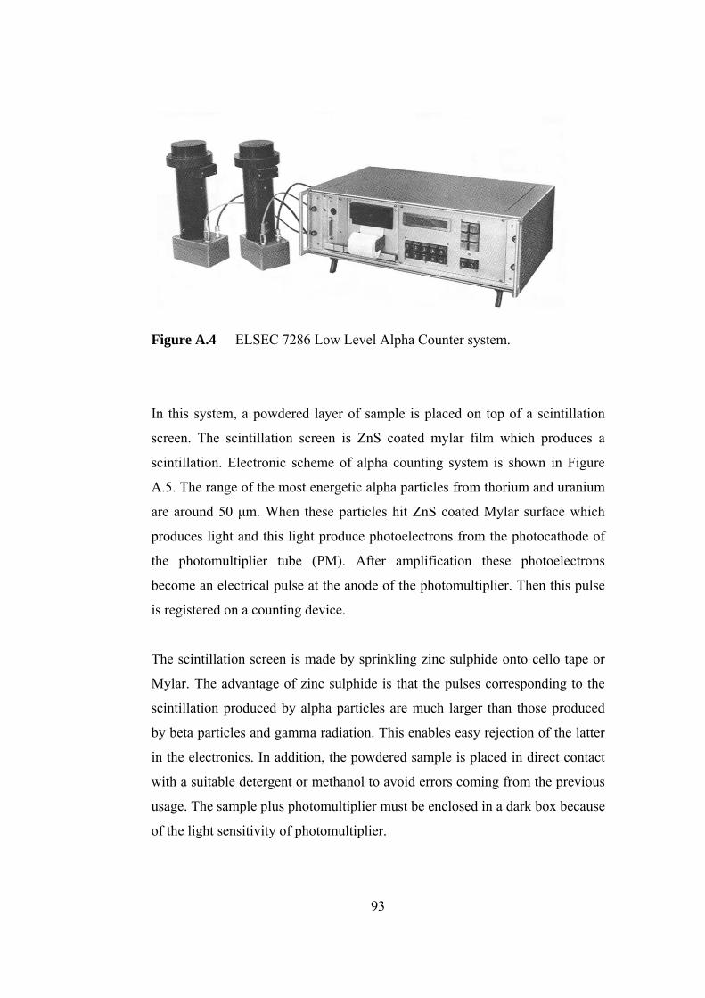
Figure A.4 ELSEC 7286 Low Level Alpha Counter system.

In this system, a powdered layer of sample is placed on top of a scintillation

screen. The scintillation screen is ZnS coated mylar film which produces a

scintillation. Electronic scheme of alpha counting system is shown in Figure

A.5. The range of the most energetic alpha particles from thorium and uranium

are around 50 μm. When these particles hit ZnS coated Mylar surface which

produces light and this light produce photoelectrons from the photocathode of

the photomultiplier tube (PM). After amplification these photoelectrons

become an electrical pulse at the anode of the photomultiplier. Then this pulse

is registered on a counting device.

The scintillation screen is made by sprinkling zinc sulphide onto cello tape or

Mylar. The advantage of zinc sulphide is that the pulses corresponding to the

scintillation produced by alpha particles are much larger than those produced

by beta particles and gamma radiation. This enables easy rejection of the latter

in the electronics. In addition, the powdered sample is placed in direct contact

with a suitable detergent or methanol to avoid errors coming from the previous

usage. The sample plus photomultiplier must be enclosed in a dark box because

of the light sensitivity of photomultiplier.

93

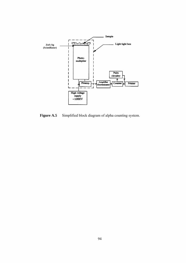
ZnS:Ag (Scintillator)

Figure A.5 Simplified block diagram of alpha counting system.

94

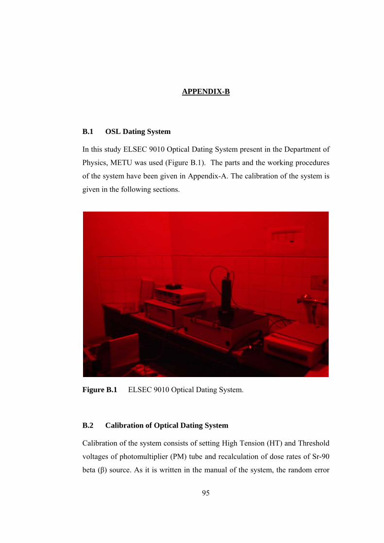
APPENDIX-B

B.1 OSL Dating System

In this study ELSEC 9010 Optical Dating System present in the Department of

Physics, METU was used (Figure B.1). The parts and the working procedures

of the system have been given in Appendix-A. The calibration of the system is

given in the following sections.

Figure B.1 ELSEC 9010 Optical Dating System.

B.2 Calibration of Optical Dating System

Calibration of the system consists of setting High Tension (HT) and Threshold

voltages of photomultiplier (PM) tube and recalculation of dose rates of Sr-90

beta (β) source. As it is written in the manual of the system, the random error

95

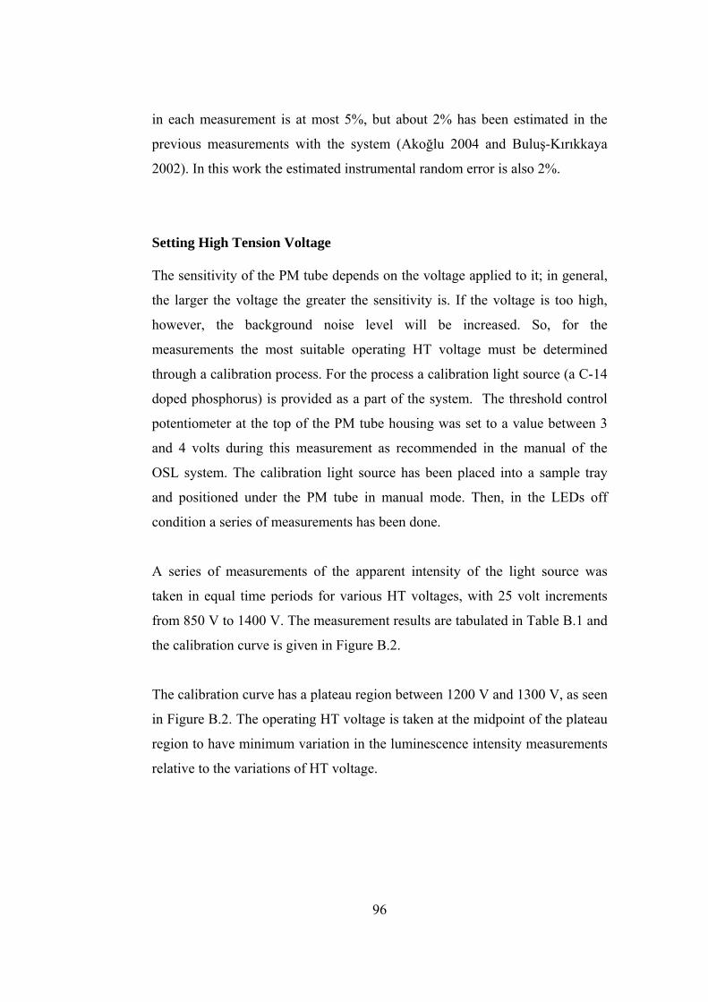
in each measurement is at most 5%, but about 2% has been estimated in the

previous measurements with the system (Akoğlu 2004 and Buluş-Kırıkkaya

2002). In this work the estimated instrumental random error is also 2%.

Setting High Tension Voltage

The sensitivity of the PM tube depends on the voltage applied to it; in general,

the larger the voltage the greater the sensitivity is. If the voltage is too high,

however, the background noise level will be increased. So, for the

measurements the most suitable operating HT voltage must be determined

through a calibration process. For the process a calibration light source (a C-14

doped phosphorus) is provided as a part of the system. The threshold control

potentiometer at the top of the PM tube housing was set to a value between 3

and 4 volts during this measurement as recommended in the manual of the

OSL system. The calibration light source has been placed into a sample tray

and positioned under the PM tube in manual mode. Then, in the LEDs off

condition a series of measurements has been done.

A series of measurements of the apparent intensity of the light source was

taken in equal time periods for various HT voltages, with 25 volt increments

from 850 V to 1400 V. The measurement results are tabulated in Table B.1 and

the calibration curve is given in Figure B.2.

The calibration curve has a plateau region between 1200 V and 1300 V, as seen

in Figure B.2. The operating HT voltage is taken at the midpoint of the plateau

region to have minimum variation in the luminescence intensity measurements

relative to the variations of HT voltage.

96

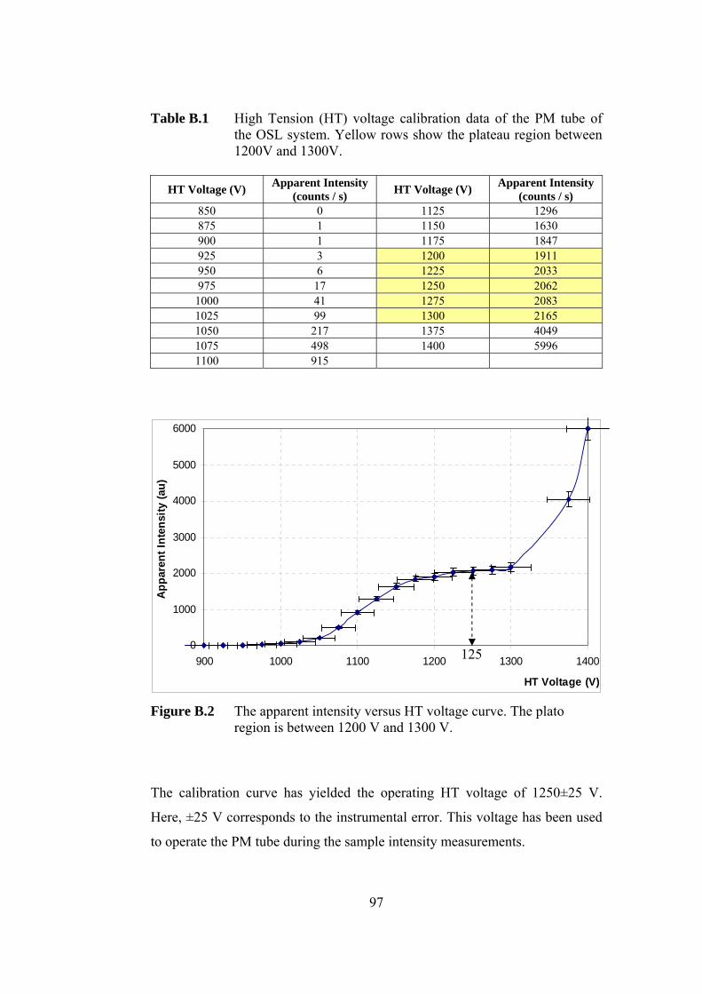
Table B.1 High Tension (HT) voltage calibration data of the PM tube of the OSL system. Yellow rows show the plateau region between 1200V and 1300V.

HT Voltage (V) Apparent Intensity (counts / s) HT Voltage (V) Apparent Intensity

(counts / s) 850 0 1125 1296 875 1 1150 1630 900 1 1175 1847 925 3 1200 1911 950 6 1225 2033 975 17 1250 2062 1000 41 1275 2083 1025 99 1300 2165 1050 217 1375 4049 1075 498 1400 5996 1100 915

0

1000

2000

3000

4000

5000

6000

900 1000 1100 1200 1300 1400

HT Voltage (V)

tt

u)y

(aen

si

Figure B.2 The apparent intensity versus HT voltage curve. The plato region is between 1200 V and 1300 V.

The calibration curve has yielded the operating HT voltage of 1250±25 V.

Here, ±25 V corresponds to the instrumental error. This voltage has been used

to operate the PM tube during the sample intensity measurements.

Appa

rent

In

125

97

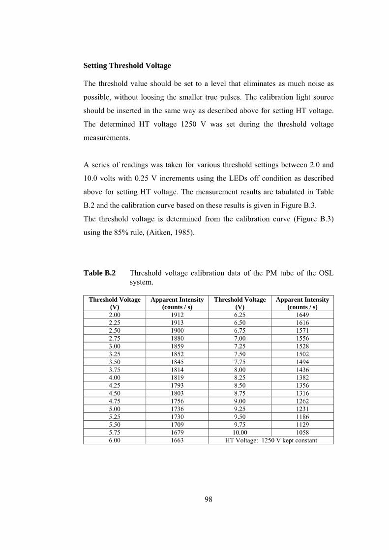
Setting Threshold Voltage

The threshold value should be set to a level that eliminates as much noise as

possible, without loosing the smaller true pulses. The calibration light source

should be inserted in the same way as described above for setting HT voltage.

The determined HT voltage 1250 V was set during the threshold voltage

measurements.

A series of readings was taken for various threshold settings between 2.0 and

10.0 volts with 0.25 V increments using the LEDs off condition as described

above for setting HT voltage. The measurement results are tabulated in Table

B.2 and the calibration curve based on these results is given in Figure B.3.

The threshold voltage is determined from the calibration curve (Figure B.3)

using the 85% rule, (Aitken, 1985).

Table B.2 Threshold voltage calibration data of the PM tube of the OSL system.

Threshold Voltage (V)

Apparent Intensity (counts / s)

Threshold Voltage (V)

Apparent Intensity (counts / s)

2.00 1912 6.25 1649 2.25 1913 6.50 1616 2.50 1900 6.75 1571 2.75 1880 7.00 1556 3.00 1859 7.25 1528 3.25 1852 7.50 1502 3.50 1845 7.75 1494 3.75 1814 8.00 1436 4.00 1819 8.25 1382 4.25 1793 8.50 1356 4.50 1803 8.75 1316 4.75 1756 9.00 1262 5.00 1736 9.25 1231 5.25 1730 9.50 1186 5.50 1709 9.75 1129 5.75 1679 10.00 1058 6.00 1663 HT Voltage: 1250 V kept constant

98

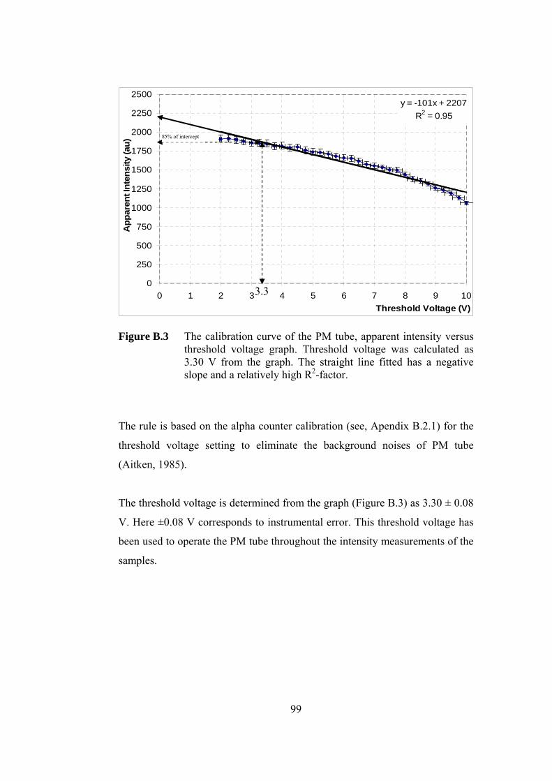
y = -101x + 2207R2 = 0.95

0

250

500

750

1000

1250

1500

1750

2000

2250

2500

0 1 2 3 4 5 6 7 8 9 1Threshold Voltage (V)

(au)

0

nte

yns

it In

tA

ppar

e

3.3

85% of intercept

Figure B.3 The calibration curve of the PM tube, apparent intensity versus threshold voltage graph. Threshold voltage was calculated as 3.30 V from the graph. The straight line fitted has a negative slope and a relatively high R2-factor.

The rule is based on the alpha counter calibration (see, Apendix B.2.1) for the

threshold voltage setting to eliminate the background noises of PM tube

(Aitken, 1985).

The threshold voltage is determined from the graph (Figure B.3) as 3.30 ± 0.08

V. Here ±0.08 V corresponds to instrumental error. This threshold voltage has

been used to operate the PM tube throughout the intensity measurements of the

samples.

99

B.3 Alpha Counting System

In this study the ELSEC 7286 Low Level Alpha Counting System (Figure A.4)

has been used. The system designed and developed specifically for dating

studies where the counting rate is small and the background noise level is very

low. See Appendix-A for its operating procedure and parts.

B.4 Calibration of Alpha Counter

Every photomultiplier tube has different characteristics, thus, the ELSEC 7286

Low Level Alpha Counter has to be calibrated before the sample

measurements. The calibration procedure is similar to that of the optical and

alpha counting systems.

Setting High Tension (HT) Voltage

As recommended in the manual, the threshold control on the back panel is set

to 1.0 V. For calibration, an alpha source which is strong enough to provide

about 10 counts per second, such as Monazite sand is needed. Monazite (Ce,

La, Y, Th)PO4 sand is the main source of thorium oxide, which contains in

amounts varying between 1 and 20 per cent thorium oxide by weight.

Commercial monazite usually contains between 3 and 9 percent thorium oxide

by weight, (Cornelius and Hurlbut, 1971). Thorium oxide is used in the

manufacture of mantles for incandescent gas lights. Monazite sand used in this

study was obtained from the burned propane lamp mantle. In addition, Sand

109 provided with the system, containing Thorium and Uranium could also be

used for the calibration. Since the Sand 109 (specified as Thorium content of

104 ppm plus Uranium content of 3.7 ppm) gives approximately 60 counts per

ksec (Aitken, 1979), the calibration process would take too much time, and

therefore it has not been preferred.

100

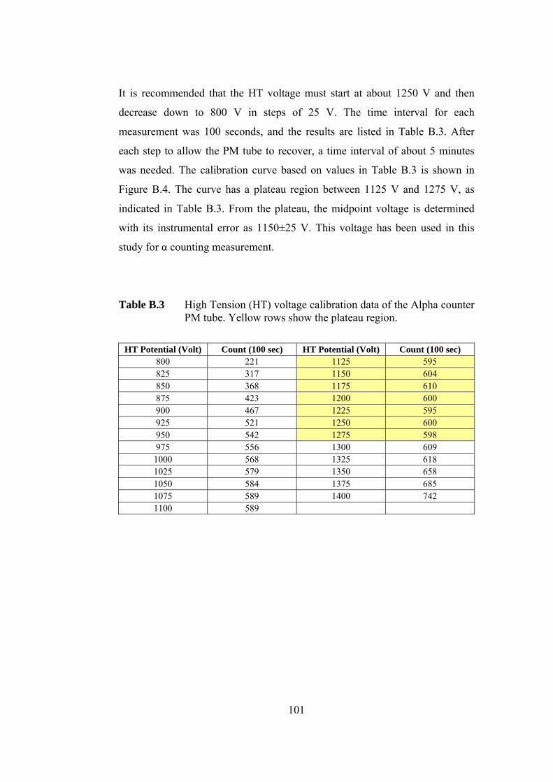
It is recommended that the HT voltage must start at about 1250 V and then

decrease down to 800 V in steps of 25 V. The time interval for each

measurement was 100 seconds, and the results are listed in Table B.3. After

each step to allow the PM tube to recover, a time interval of about 5 minutes

was needed. The calibration curve based on values in Table B.3 is shown in

Figure B.4. The curve has a plateau region between 1125 V and 1275 V, as

indicated in Table B.3. From the plateau, the midpoint voltage is determined

with its instrumental error as 1150±25 V. This voltage has been used in this

study for α counting measurement.

Table B.3 High Tension (HT) voltage calibration data of the Alpha counter PM tube. Yellow rows show the plateau region.

HT Potential (Volt) Count (100 sec) HT Potential (Volt) Count (100 sec) 800 221 1125 595 825 317 1150 604 850 368 1175 610 875 423 1200 600 900 467 1225 595 925 521 1250 600 950 542 1275 598 975 556 1300 609 1000 568 1325 618 1025 579 1350 658 1050 584 1375 685 1075 589 1400 742 1100 589

101

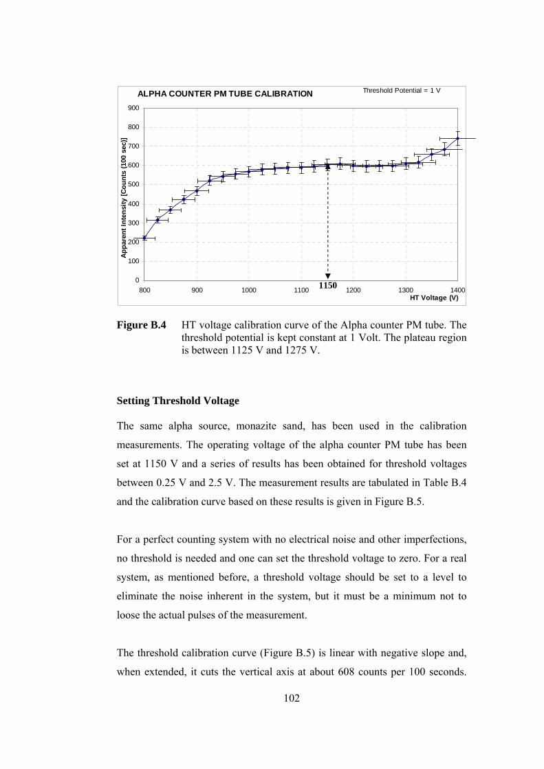
ALPHA COUNTER PM TUBE CALIBRATION

0

100

200

300

400

500

600

700

800

900

800 900 1000 1100 1200 1300 1400HT Voltage (V)

Figure B.4 HT voltage calibration curve of the Alpha counter PM tube. The threshold potential is kept constant at 1 Volt. The plateau region is between 1125 V and 1275 V.

Setting Threshold Voltage

The same alpha source, monazite sand, has been used in the calibration

measurements. The operating voltage of the alpha counter PM tube has been

set at 1150 V and a series of results has been obtained for threshold voltages

between 0.25 V and 2.5 V. The measurement results are tabulated in Table B.4

and the calibration curve based on these results is given in Figure B.5.

For a perfect counting system with no electrical noise and other imperfections,

no threshold is needed and one can set the threshold voltage to zero. For a real

system, as mentioned before, a threshold voltage should be set to a level to

eliminate the noise inherent in the system, but it must be a minimum not to

loose the actual pulses of the measurement.

The threshold calibration curve (Figure B.5) is linear with negative slope and,

when extended, it cuts the vertical axis at about 608 counts per 100 seconds.

Apn

ten

y [C

t00

pare

t In

sit

oun

s (1

sec

)]

Threshold Potential = 1 V

1150

102

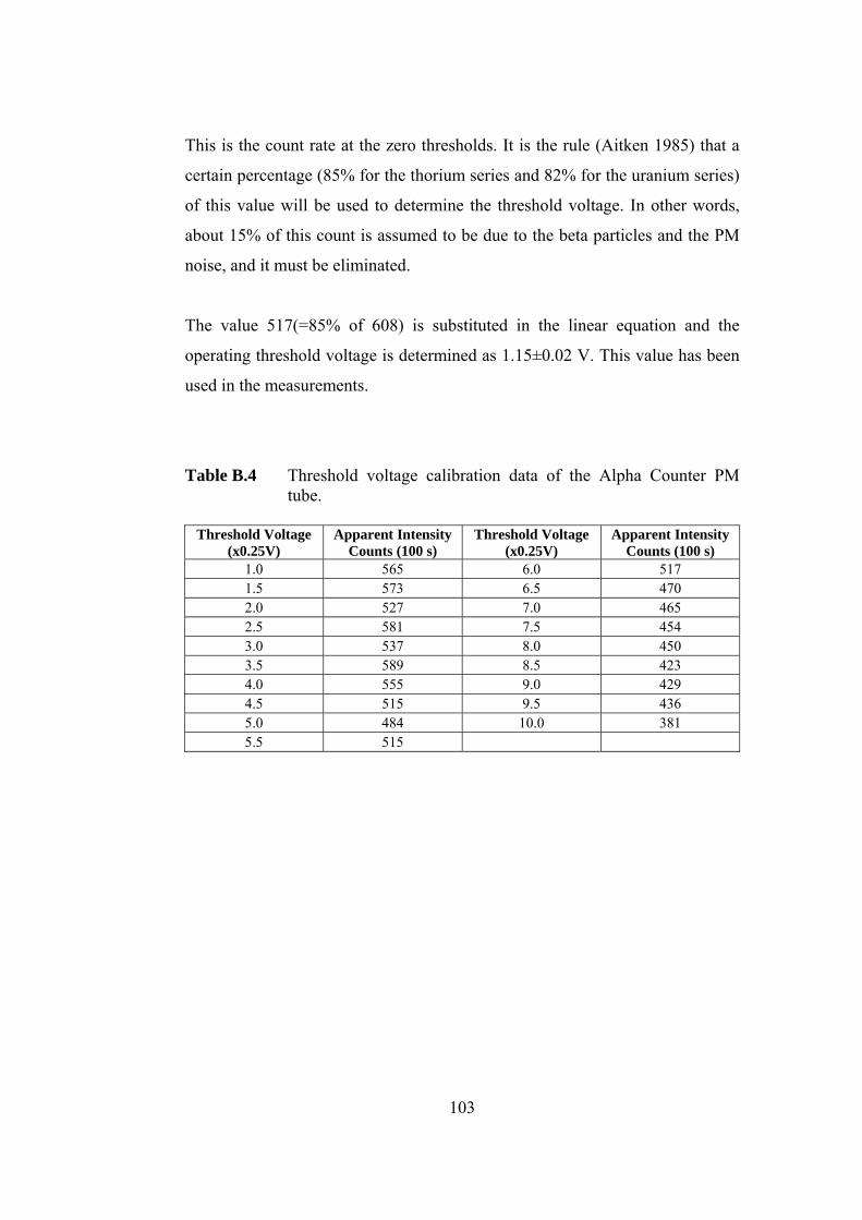
This is the count rate at the zero thresholds. It is the rule (Aitken 1985) that a

certain percentage (85% for the thorium series and 82% for the uranium series)

of this value will be used to determine the threshold voltage. In other words,

about 15% of this count is assumed to be due to the beta particles and the PM

noise, and it must be eliminated.

The value 517(=85% of 608) is substituted in the linear equation and the

operating threshold voltage is determined as 1.15±0.02 V. This value has been

used in the measurements.

Table B.4 Threshold voltage calibration data of the Alpha Counter PM tube.

Threshold Voltage (x0.25V)

Apparent Intensity Counts (100 s)

Threshold Voltage (x0.25V)

Apparent Intensity Counts (100 s)

1.0 565 6.0 517 1.5 573 6.5 470 2.0 527 7.0 465 2.5 581 7.5 454 3.0 537 8.0 450 3.5 589 8.5 423 4.0 555 9.0 429 4.5 515 9.5 436 5.0 484 10.0 381 5.5 515

103

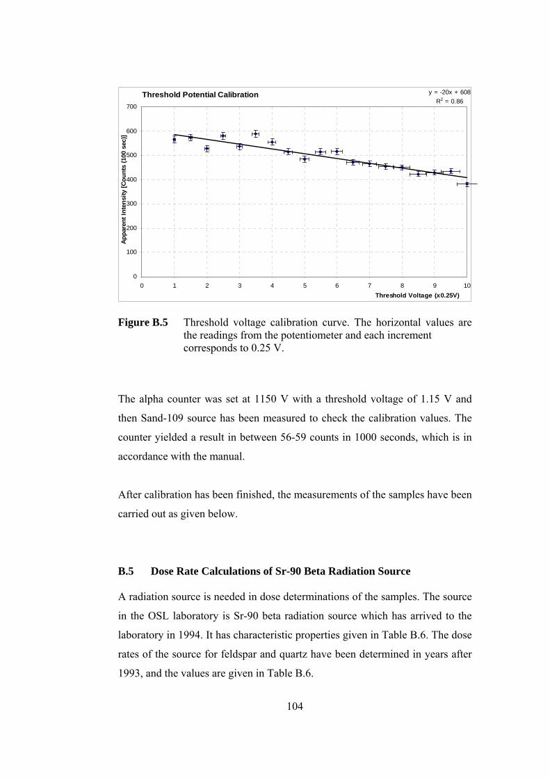
Figure B.5 Threshold voltage calibration curve. The horizontal values are the readings from the potentiometer and each increment corresponds to 0.25 V.

The alpha counter was set at 1150 V with a threshold voltage of 1.15 V and

then Sand-109 source has been measured to check the calibration values. The

counter yielded a result in between 56-59 counts in 1000 seconds, which is in

accordance with the manual.

After calibration has been finished, the measurements of the samples have been

carried out as given below.

B.5 Dose Rate Calculations of Sr-90 Beta Radiation Source

A radiation source is needed in dose determinations of the samples. The source

in the OSL laboratory is Sr-90 beta radiation source which has arrived to the

laboratory in 1994. It has characteristic properties given in Table B.6. The dose

rates of the source for feldspar and quartz have been determined in years after

1993, and the values are given in Table B.6.

4.5

517

Threshold Potential Calibration y = -20x + 608R2 = 0.86

0

100

200

300

400

500

600

700

0 1 2 3 4 5 6 7 8 9 10Threshold Voltage (x0.25V)

p I

si1

c00

se

ty [C

ount

s (

nten

pare

ntA

)]

104

The dose rates of the source depend on time and therefore the present value of

the dose rate must be determined prior to each measurement. In this work the

values of the year 2004 are used, and they are based on the 2001 values (Buluş-

Kırıkkaya, 2002).

A radioactive nuclide, like Sr-90, decays with time t according to the law of

radioactive decay.

teN)t(N λ−= 0 (B.1)

where, N0 is the number of radioactive nuclei in the sample at t=0 and N(t) is

the number remaining at any later time t. The decay constant (or disintegration

constant) λ has a characteristic value for every radionuclide. It is related to the

half-life t1/2 as

21

2tln

=λ (B.2)

where, t1/2 =28 years for Sr-90.

The decay rate R(=-dN/dt) is more often used than N(t). Differentiating

Equation 3-1, we find

teNdt

)t(dN)t(R λλ −=−= 0

or

teR)t(R λ−= 0 (B.3)

105

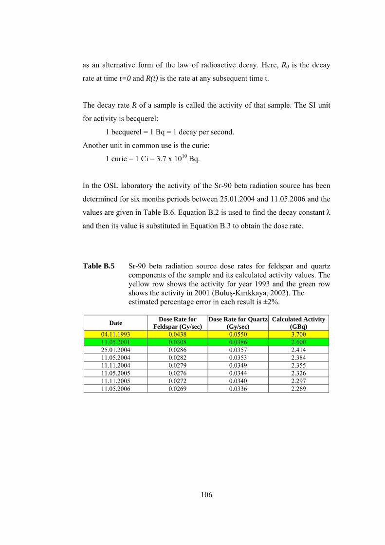
as an alternative form of the law of radioactive decay. Here, R0 is the decay

rate at time t=0 and R(t) is the rate at any subsequent time t.

The decay rate R of a sample is called the activity of that sample. The SI unit

for activity is becquerel:

1 becquerel = 1 Bq = 1 decay per second.

Another unit in common use is the curie:

1 curie = 1 Ci = 3.7 x 1010 Bq.

In the OSL laboratory the activity of the Sr-90 beta radiation source has been

determined for six months periods between 25.01.2004 and 11.05.2006 and the

values are given in Table B.6. Equation B.2 is used to find the decay constant λ

and then its value is substituted in Equation B.3 to obtain the dose rate.

Table B.5 Sr-90 beta radiation source dose rates for feldspar and quartz components of the sample and its calculated activity values. The yellow row shows the activity for year 1993 and the green row shows the activity in 2001 (Buluş-Kırıkkaya, 2002). The estimated percentage error in each result is ±2%.

Date Dose Rate for Feldspar (Gy/sec)

Dose Rate for Quartz (Gy/sec)

Calculated Activity (GBq)

04.11.1993 0.0438 0.0550 3.700 11.05.2001 0.0308 0.0386 2.600 25.01.2004 0.0286 0.0357 2.414 11.05.2004 0.0282 0.0353 2.384 11.11.2004 0.0279 0.0349 2.355 11.05.2005 0.0276 0.0344 2.326 11.11.2005 0.0272 0.0340 2.297 11.05.2006 0.0269 0.0336 2.269

106

REFERENCES

Aitken M.J., (1979). Values observed at Research Lab for Archaeology and the History of art, Oxford University (7286 Low Level Alpha Counter User Manual). Aitken M.J. (1985). Thermoluminescence Dating. Academic Press, London, 359p. ISBN: 0-12-046380-6. Aitken, M.J., (1989). Luminescence dating: a guide for non-specialists. Archaeometry 31, 2, 147-159. Aitken M.J. (1998). An introduction to optical dating .The Dating of Quaternary Sediments by the Use of Photon-Stimulated Luminescence. Oxford University Press, Oxford, 267p., ISBN: 0-19-854092-2. Akoğlu K.G., (2003). M.Sc. Thesis: Optically Stimulated Luminescence (OSL) Dating of Çatalhöyük Samples. METU Graduate School of Natural and Applied Sciences. Auclair M., Lamothe M. and Huot S. (2003). Measurement of anomalous fading for feldspar IRSL using SAR. Radiation Measurements 37, 487-492. Berger G.W. and Huntley D.J. (1994). Tests for optically stimulated luminescence from tephra glass. Quaternary Geochronology (Quaternary Science Reviews) 13, 509-511. Berger G.W. and Neil P.A. (1999). Photon-stimulated-luminescence (PSL) dating tests of glass-rich volcanic ash. Book of Abstract LED99: 138. Black C.A., (1965). Method of Soil Analysis (part 2) Chemical and Microbiological Properties. American Society of Agromony.

Bøtter-Jensen L., (2000). Development of Optically Stimulated Luminescence Techniques using Natural Minerals and Ceramics, and their Application to Retrospective Dosimetry. Risø National Laboratory, Roskilde. ISBN 87-550-2755-5 Bøtter-Jensen L., Solongo S., Murray A. S., Banerjee D. and Jungner H. (2000). Using the OSL single-aliquot regenerative-dose protocol with quartz extracted from building materials in retrospective dosimetry. Radiation Measurements 32, 841-845 Bøtter-Jensen L., McKeever S.W.S. and Wintle A.G. (2003a). Optically Stimulated Luminescence Dosimetry. Elsevier Science, The Netherlands, 355p., ISBN: 0-444-50684-5. Bøtter-Jensen L., Andersen C.E., Duller G.A.T. and Murray A.S. (2003b). Developments in radiation, stimulation and observation facilities in luminescence measurements. Radiation Measurements 37, 535-541. Bulur E., (1996). An alternative technique for optically stimulated luminescence (OSL) experiment. Radiation Measurements 26, 701-709. Bulur E. and Göksu H. Y., (1997). Pulsed optically stimulated luminescence from α-Al2O3:C using green light emitting diyotes. Radiation Measurements, 27, 479-488. Bulur E. and Göksu H. Y., (1999). Infrared (IR) stimulated luminescence from feldspars with linearly increasing excitation light intensity. Radiation Measurement 30, 505-512. Buluş-Kırıkkaya E., (2002). Ph.D. Thesis: Kocaeli (Kullar-Yaylacık) Fayından Alınan Kuvars Örneklerinin Optik Uyarmalı Lüminesans (OSL) ve Termolüminesans (TL) Yöntemleri ile İncelenmesi. Kocaeli Üniversitesi Fizik Bölümü. Chen R. and McKeever S.W.S. (1997). Theory of thermoluminescence and related phenomena. World Scientific Publishing, Singapore, 559p., ISBN: 9810222955.

Clark P.A. and Templer R.H. (1988). Thermoluminescence dating of materials which exhibit anomalous fading. Archaeometry 30, 19-36. Cornelius S. Hurlbut, JR. (1971). Dana’s Manual of Mineralogy. Wiley International Edition, Newyork, 579p., ISBN: 0-471-42225-8. Duller G.A.T. (1991). Equivalent dose determination using single aliquots. Nuclear Tracks and Radiation Measurements 18, 371-378. Duller G.A.T., Botter-Jensen L. and Markey B.G., (1997). A Luminescence Imaging System Based on a CCD Camera. Radiation Measurements 27, 91-99. Duller G. A. T., Bøtter-Jensen L., Murray A. S. and Truscott A. J., (1999). Single grain laser luminescence (SGLL) measurements using a novel automated reader Nuclear Instruments and Methods in Physics Research Section B: Beam Interactions with Materials and Atoms, 155, 506-514 Fleming S., (1979). Thermoluminescence techniques in archaeology. Oxford University Pres, London, 212p., ISBN: 0-19-859929-3. Fragoulis D. and Stoebe T.G. (1990). Relationship of anomalous fading to feldspar inclusions in quartz. Radiation Protection Dosimetry 34, 65-68. Fragoulis D.V. and Readhead M.L. (1991). Feldspar inclusions and the anomalous fading and enhancement of thermoluminescence in quartz grains. Nuclear Tracks and Radiation Measurements 18, 291-296. Franklin A.D., Prescott J.R. and Scholefield R.B. (1995). The mechanism of thermoluminescence in an Australian sedimentary quartz. Journal of Luminescence 63, 317-326. Forman, S. L., and Pierson, J., (2003). Formation of linear and parabolic dunes on the eastern Snake River Plain, Idaho in the nineteenth century: Geomorphology, v. 1354, 1-12. Huntley D.J., Godfrey-Smith D.I. and Thewalt M.L.W. (1985). Optical dating of sediments. Nature, 313, 105-107.

Huntley D.J., Hutton J.T. and Prescott J.R. (1993). The stranded beach-dune sequence of south-east South Australia: A test of thermoluminescence dating, 0-800 ka. Quaternary Science Reviews 12, 1-20. Huntley D.J., Hutton J.T. and Prescott J.R. (1994). Further thermoluminescence dates from the dune sequence in the southeast of South Australia. Quaternary Science Reviews 13, 201-207. Huntley D.J. and Prescott J.R. (2001). Improved methodology and new thermoluminescence ages for the dune sequence in south-east South Australia. Quaternary Science Reviews 20, 687-699. Hütt G., Jaek I. and Tchonka J., (1988). Optical Dating: K-Feldspars Optical Response Stimulation Spectra. Quaternary Science Reviews 7, 381-385. Lamothe M., Auclair M., Hamzaoui C. and Huot S. (2003). Towards a prediction of long-term anomalous fading of feldspar IRSL. Radiation Measurements 37, 493-498. Lang A., Lindauer S., Kuhn R. and Wagner G.A. (1996). Procedures used for Optically and Infrared Stimulated Luminescence Dating of Sediments in Heidelberg. Ancient TL 14, 7-11. Liritzis I. and Vafiadou A., (2005). Dating by Luminescence of Ancient Megalithic Masonry. Mediterranean Archaeology and Archaeometry 5, No 1, 25-38 McKeever S.W.S., (1985). Thermoluminescence of solids. Cambridge University Press, London, 376p. ISBN: 0-521-36811-1. McKeever S. W. S., Alselrod M. S. and Markey B. G., (1996). Pulsed optically stimulated luminescence dosimetry using α-Al2O3:C. Radiation Protection Dosimetry, 65, 267–72. McKeever S.W.S., Botter-Jensen L., Larsen N.A. and Duller G.A.T., (1997). Temperature Dependence of OSL Decay Curves: Experimental and Theoretical Aspects. Radiation Measurements 27. 161-170.

Pliny (AD77). Pliny online: complete translation, by John Bostock and H. T Riley (1855). http://www.perseus.tufts.edu/cgi-bin/ptext?lookup=Plin.+Nat.+toc Poolton N.R.J., Botter-Jensen L. and Johnson O., (1995). Thermo-Optical Properties of Optically Stimulated Luminescence in Feldspars. Radiation Measurements 24, 531-534. Prescott J.R. and Robertson G.B. (1997). Sediment dating by luminescence: a review. Radiation Measurements 27, 893-922. Readhead M.L. (1988). Thermoluminescence dating study of quartz in aeolian sediments from southeastern Australia. Quaternary Science Reviews 7, 257-264. Rhodes E.J. (1988). Methodological considerations in the optical dating of quartz. Quaternary Science Reviews 7, 395-400. Rhodes E.J. (1990). Optical dating of quartz from sediments. Unpublished D.Phil. Thesis, Oxford University. Roberts R.G., Jones R., Spooner N.A., Head M.J., Murray A.S. and Smith M.A. (1994). The human colonisation of Australia: optical dates of 53,000 and 60,000 years bracket human arrival at Deaf Adder George, Northern Territory. Quaternary Geochronology (Quaternary Science Reviews) 13, 575-583. Roberts R.G. (1997). Luminescence dating in archaeology: from origins to optical. Radiation Measurements 27, 819-892. Smith B.W., Aitken M.J., Rhodes E.J., Robinson P.D. and Geldard D.M. (1986). Optical dating: methodological aspects. Radiation Protection Dosimetry 17, 229-233. Smith B.W. (1988). Zircon from sediments: a combined OSL and TL auto regenerative dating technique. Quaternary Science Reviews 7, 401-406. Spooner N.A. (1992). Optical dating: preliminary results on the anomalous fading of luminescence from feldspars. Quaternary Science Reviews 11, 139-145.

Spooner N.A. (1994). The anomalous fading of infra-red stimulated luminescence from feldspars. Radiation Measurements 23, 625-632. Stokes S. (1992). Optically dating of young (modern) sediments using quartz: Result from a selection of depositional environments. Quaternary Science Reviews 11, 153-159. Stoneham D., (1991). Authenticity testing. In: Scientific Dating Methods, eds. H.Y. Göksu, M. Oberhofer and D. Regulla, Eurocourses Advanced Scientific Techniques 1, 175-192, Kluwer Academic Publishers, Dordrecht. XLII References Şimşek C., (2004). 2003 Yılı Laodikeia Antik Kenti Kazısı, 26. Kazı Sonuçları Toplantısı 1, 305-320. ISBN: 975-17-3149-6 (Tk.No) 975-17-3150-X (1. Cilt) Taylor R. E. and Aitken M.J., (1997). eds. Chronometric Dating in Archaeology . Advances in Archaeological and Museum Science, vol. 2. New York: Plenum Press, 1997. xix + 395 pp. Vandenberghe D., (2003). Ph.D. Thesis: Investigation of the Optically Stimulated Luminescence Dating Method for Application to Young Gelogical Sediments. Department of Analytical Chemistry Institute for Nuclear Sciences, Universiteit Gent. Vancraeynest L., (1998). Bijdrage tot de studie van de tehrmoluminescentie-dateringsmethode en toepassing op archeologisch keramiek en eolische sedimenten. Doctoraatsthesis, Universiteit Gent. Visocekas R., Ceva T., Marti C., Lefaucheux F., and Robert M.C., (1976). Tunneling processes in afterglow of calcite. Physica Status Solidi A 35, 315-327. Visocekas R. (2000). Monitoring anomalous fading of TL of feldspars by using far-red emission as a gauge. Radiation Measurements 32, 499-504. Wagner G.A., (1995). Altersbestimmung von jungen Gesteinen und Artefakten: Physikalische und chemische Uhren in Quartärgeologie und Archäologie. Enke-Verlag, Stuttgart, 277p., ISBN: 3-432-26411-9. XLVI References

Wagner G.A., (1998). Age determination of young rocks and artifacts: physical and chemical clocks in Quaternary geology and archaeology. Springer-Verlag Berlin Heidelberg, 466p., ISBN: 3-540-63436-3. Wilkinson A.J. (1997). Theoretical Simulation of Preheat-OSL Cycles. Radiation Measurements 27, 489-497. Wintle A.G., Aitken M.J. and Huxtable J. (1971). Abnormal thermoluminescence fading characteristics. In: Proceedings of the third international conference on luminescence dosimetry (ed.: Mejdahl V.), 14/11/1974, Risø, Denmark. Risø Report 249, 105-131. Wintle A.G. (1973). Anomalous fading of thermoluminescence in mineral samples. Nature 245, 143-144. Wintle A.G. (1977). Detailed study of a thermoluminescent mineral exhibiting anomalous fading. Journal of Luminescence 15, 385-393. Wolfe S.A., Huntley D.J., and Ollerhead J. (1995). Recent and late Holocene sand dune activity in southwestern Saskatchewan. In current research 1995-B; Geological Survey of Canada, 131-140. Yurdatapan E., (1997). M.Sc. Thesis: Optically stimulated luminescence (OSL) and its applications to archaeological materials: a pilot study. METU Graduate School of Natural and Applied Sciences. Zimmerman J., (1971). The radiation-induced increase of thermoluminescence sensitivity of fired quartz. Journal of Physics C: Solid state physics 4, 3277-3291.

VITA

PERSONAL INFORMATION

Surname, Name: Demirtürk, Tayfun

Date and Place of Birth: June 22nd , 1964, Acıpayam-DENİZLİ

e-mail: z7f79@yahoo.com

EDUCATION

Degree Institution

MS Texas Tech University, Lubbock, TX, USA (1994-1997)

BS Ankara University, Ankara (1982-1986)

High School Şarkışla Lisesi, Sivas (1978-1981)

PUBLICATION LIST

1. M. Özbakan, A. Özer, T. Demirtürk, (2006). Optik Uyarmalı Lüminesans

Tekniği ile Laodikeia (Denizli/Türkiye) Yapı Seramiklerinin İncelenmesi.

T.C. Kültür ve Turizm Bakanlığı Yayınları: XXI. Arkeometri Sonuçları

Toplantısı, Yayın No: 3052, 87-96, Ankara. ISBN: 975-17-3191-7

2. T. Demirtürk, M. Özbakan, A. Özer, (3-7 May 2004). Dating of Laodikeia

(Denizli) Building Ceramics Using Optically Stimulated Luminescence

(OSL) Techniques. 34th International Symposium on Archaeometry,

Zaragoza (Spain).