Databases in 88 Pages - · PDF fileDatabases in 88 Pages Aarne Ranta CSE, Chalmers University...
88
Databases in 88 Pages Aarne Ranta CSE, Chalmers University of Technology and University of Gothenburg 1
Transcript of Databases in 88 Pages - · PDF fileDatabases in 88 Pages Aarne Ranta CSE, Chalmers University...

Databases in 88 Pages
Aarne Ranta
CSE, Chalmers University of Technology and University ofGothenburg
1

Contents
1 Introduction* 71.1 Data vs. programs . . . . . . . . . . . . . . . . . . . . . . . . . . 71.2 A short history of databases . . . . . . . . . . . . . . . . . . . . . 71.3 SQL . . . . . . . . . . . . . . . . . . . . . . . . . . . . . . . . . . 81.4 DBMS . . . . . . . . . . . . . . . . . . . . . . . . . . . . . . . . . 91.5 Course contents . . . . . . . . . . . . . . . . . . . . . . . . . . . . 91.6 The big picture . . . . . . . . . . . . . . . . . . . . . . . . . . . . 12
2 Data modelling with relations 132.1 Relations and tables . . . . . . . . . . . . . . . . . . . . . . . . . 132.2 Operations on relations . . . . . . . . . . . . . . . . . . . . . . . 152.3 Multiple tables and joins . . . . . . . . . . . . . . . . . . . . . . . 162.4 Referential constraints . . . . . . . . . . . . . . . . . . . . . . . . 172.5 Key and uniqueness constraints . . . . . . . . . . . . . . . . . . . 172.6 Multiple values . . . . . . . . . . . . . . . . . . . . . . . . . . . . 182.7 Null values . . . . . . . . . . . . . . . . . . . . . . . . . . . . . . 19
3 Entity-Relationship diagrams 203.1 E-R syntax . . . . . . . . . . . . . . . . . . . . . . . . . . . . . . 203.2 From description to E-R . . . . . . . . . . . . . . . . . . . . . . . 213.3 Converting E-R diagrams to database schemas . . . . . . . . . . 223.4 Using the Query Converter* . . . . . . . . . . . . . . . . . . . . . 24
4 Functional dependencies and normal forms 274.1 The design workflow . . . . . . . . . . . . . . . . . . . . . . . . . 274.2 Examples of dependencies and normal forms . . . . . . . . . . . . 28
4.2.1 Functional dependencies, keys, and superkeys . . . . . . . 284.2.2 BCNF . . . . . . . . . . . . . . . . . . . . . . . . . . . . . 294.2.3 3NF . . . . . . . . . . . . . . . . . . . . . . . . . . . . . . 304.2.4 4NF . . . . . . . . . . . . . . . . . . . . . . . . . . . . . . 304.2.5 A bigger example . . . . . . . . . . . . . . . . . . . . . . . 314.2.6 One more example: FD or MVD? . . . . . . . . . . . . . 32
4.3 Mathematical definitions of dependencies . . . . . . . . . . . . . 334.4 Definitions of closures, keys, and superkeys . . . . . . . . . . . . 344.5 Definitions and algorithms for normal forms . . . . . . . . . . . . 344.6 Relation analysis in the Query Converter* . . . . . . . . . . . . . 374.7 Further reading on normal forms and functional dependencies* . 37
5 SQL 385.1 SQL in a nutshell . . . . . . . . . . . . . . . . . . . . . . . . . . . 385.2 Database and table definitions . . . . . . . . . . . . . . . . . . . 405.3 Inserting values . . . . . . . . . . . . . . . . . . . . . . . . . . . . 425.4 Query usage and semantics: simple queries . . . . . . . . . . . . 43
5.4.1 The cartesian product (FROM) . . . . . . . . . . . . . . . 43
2

5.4.2 The condition on attributes (WHERE) . . . . . . . . . . . 445.4.3 The projected tuples (SELECT) . . . . . . . . . . . . . . 455.4.4 Set operations on queries (UNION, INTERSECT, EX-
CEPT) . . . . . . . . . . . . . . . . . . . . . . . . . . . . 465.5 Query usage and semantics: more complex queries . . . . . . . . 46
5.5.1 Local definitions (WITH) . . . . . . . . . . . . . . . . . . 465.5.2 Sorting (ORDER BY) . . . . . . . . . . . . . . . . . . . . 475.5.3 Grouping (GROUP BY) and group conditions (HAVING) 475.5.4 Join operations (JOIN) . . . . . . . . . . . . . . . . . . . 495.5.5 Pattern matching (LIKE) . . . . . . . . . . . . . . . . . . 51
5.6 Views (CREATE VIEW) . . . . . . . . . . . . . . . . . . . . . . 515.7 SQL pitfalls . . . . . . . . . . . . . . . . . . . . . . . . . . . . . . 515.8 SQL in the Query Converter* . . . . . . . . . . . . . . . . . . . . 53
6 Table modification and triggers 546.1 Active element hierarchy . . . . . . . . . . . . . . . . . . . . . . . 546.2 Referential constraints and policies . . . . . . . . . . . . . . . . . 556.3 CHECK constraints . . . . . . . . . . . . . . . . . . . . . . . . . 566.4 ALTER TABLE . . . . . . . . . . . . . . . . . . . . . . . . . . . 576.5 Triggers . . . . . . . . . . . . . . . . . . . . . . . . . . . . . . . . 57
7 Relational algebra and query compilation 607.1 The compiler pipeline . . . . . . . . . . . . . . . . . . . . . . . . 607.2 Relational algebra . . . . . . . . . . . . . . . . . . . . . . . . . . 607.3 Variants of algebraic notation . . . . . . . . . . . . . . . . . . . . 627.4 From SQL to relational algebra . . . . . . . . . . . . . . . . . . . 62
7.4.1 Basic queries . . . . . . . . . . . . . . . . . . . . . . . . . 627.4.2 Grouping and aggregation . . . . . . . . . . . . . . . . . . 637.4.3 Sorting and duplicate removal . . . . . . . . . . . . . . . . 65
7.5 Query optimization . . . . . . . . . . . . . . . . . . . . . . . . . . 657.5.1 Algebraic laws . . . . . . . . . . . . . . . . . . . . . . . . 657.5.2 Example: pushing conditions in cartesian products . . . . 66
7.6 Relational algebra in the Query Converter* . . . . . . . . . . . . 66
8 SQL in software applications 678.1 SQL as a part of a bigger program . . . . . . . . . . . . . . . . . 678.2 A minimal JDBC program* . . . . . . . . . . . . . . . . . . . . . 678.3 Building queries and updates from input data* . . . . . . . . . . 698.4 SQL injection . . . . . . . . . . . . . . . . . . . . . . . . . . . . . 708.5 The ultimate query language?* . . . . . . . . . . . . . . . . . . . 71
9 Remaining SQL topics: transactions, authorization, indexes 739.1 Authorization and grant diagrams . . . . . . . . . . . . . . . . . 739.2 Transactions . . . . . . . . . . . . . . . . . . . . . . . . . . . . . 749.3 Interferences and isolation levels . . . . . . . . . . . . . . . . . . 759.4 Indexes . . . . . . . . . . . . . . . . . . . . . . . . . . . . . . . . 76
3

10 Alternative data models 7910.1 XML and its data model . . . . . . . . . . . . . . . . . . . . . . . 7910.2 The XPath query language . . . . . . . . . . . . . . . . . . . . . 8310.3 XML and XPath in the query converter . . . . . . . . . . . . . . 8310.4 NoSQL data models* . . . . . . . . . . . . . . . . . . . . . . . . . 8410.5 The Cassandra DBMS and its query language CQL* . . . . . . . 8410.6 Further reading on NoSQL* . . . . . . . . . . . . . . . . . . . . . 87
4
Preface to second edition
These notes are the same as in 2016, with small additions and corrections to beexpected during the course.
Gothenburg, 23 February 2017
Aarne Ranta
Preface
These are notes for a databases course (TDA357/DIT620) taught in Gothenburgin 2016. They cover the material presented during the lectures. Similar materialcan also be found from course slides written by previous teachers. However, mypersonal preference is to use the blackboard rather than slides. This gives abetter guarantee that the students (let alone the teacher) don’t fall asleep. Italso forces the lectures to have a natural, relaxed pace, with not too muchinformation. For reading outside the lectures, a complete text works betterthan slides.
Just like slides published on course web sites, these course notes shouldeliminate the need to take your own notes about everything. Then you canconcentrate more on listening and thinking. The best way to use these notes isto read them both before and after each lecture. Then you will be prepared forthe material and maybe develop some questions in advance.
Even though these notes thus replace the slides, there are any number ofthings they don’t replace:• The course book. It has much more examples, explanations, and argu-
mentation than this little compendium.• The lectures. Attending the lectures should increase your understanding.
However, reading these notes may compensate skipping a lecture or twofor intance because of illness.
• Practice. To build a proper understanding, you must build and use yourown database on a computer. You must also solve some theoretical prob-lems by pencil and paper. The course assignments and exercises will helpyou get this practice - provided you do them yourself!
We will use a running example that deals with geographical data: countriesand their capitals, neighbours, currencies, and so on. This is a bit different frommany other slides, books, and articles. In them, you can find examples such ascourse descriptions, employer records, and movie databases. To my mind, suchexamples feel more difficult since they are not common knowledge. This meansthat, when learning new mathematical and programming concepts, you haveto learn new content at the same time. I find it easier to study new technicalmaterial if the contents are familiar. For instance, it is easier to test a querythat is supposed to assign ”Paris” to ”the capital of France” than a query thatis supposed to assign ”60,000” to ”the salary of John Johnson”. There is simplyone thing less to keep in mind. It also eliminates to show example tables allthe time, because we can simply refer to ”the table containing all European
5
countries and their capitals”, which most readers will have clear enough in theirminds. Of course, we will have the occasion to show other kinds of databases aswell. The country database does not have all the characteristics that a databasemight have, for instance, very rapid changes in the data.
This compendium proceeds in the order of the lectures. It is being writtenduring the course. My aim is to make every chapter available before the cor-responding lecture is given. But I may also make corrections after the lecture.The sections marked with an asterisk (*) are ones that will not be needed forthe exam in Spring 2016.
The material has been inspired by the course book (Garcia-Molina, Ullman,and Widom, Database systems: The Complete Book), by earlier course mate-rial by Niklas Broberg and Graham Kemp, as well as by notes (in Finnish) byJyrki Nummenmaa. I am grateful to Jyrki Nummenmaa and Gregoire Detrezon general advice and comments on the contents, and to Simon Smith, AdamIngmansson, and Viktor Blomqvist for comments during the course. More com-ments, corrections, and suggestions are therefore most welcome - your name willbe added here if you don’t object!
Gothenburg, March 2016
Aarne Ranta
6

1 Introduction*
This chapter is an overview of the field of databases and of this course. Inaddition to the material printed here, the lecture will also talk about practicalquestions such as assignments, exercises, and the exam. This information canbe found on the course web page. The goal of this chapter (and the whole firstlecture) is to give you a clear picture of what you are expected to do and learnduring the course.
1.1 Data vs. programs
Computers run programs that process data. Sometimes this data comes fromuser interaction and is thrown away after the program is run. But often thedata must be stored for a longer time, so that it can be accessed again. Banks,for instance, have to store the data about bank accounts so that no penny islost.
It is typical that data lives much longer than the programs that process it:decades rather than just years. Programs, even programming languages, maybe changed every five years or so. On the other hand, while data is maintainedfor decades, it may also be changed very rapidly. For instance, a bank can havemillions of transactions daily, coming from ATM’s, internet purchases, etc. Thismeans that account balances must be continuously updated. At the same time,the history of transactions must be kept for years.
A database is any collection of data that can be accessed and processedby computer programs. It must support both updates (i.e. changes in thedata) and queries (i.e. questions about the data). It must be structured sothat these operations can be performed efficiently and accurately. For instance,English texts describing the data would be both too slow and too inaccurate.But the structure must also be generic enough so that it can be accessed indifferent ways. For instance, the data structures of some advanced programminglanguage may be too hard to access from programs written in other languages.
1.2 A short history of databases
When databases came to wide use, for instance in banks in the 1960’s, they werenot yet standardized. They could be vendor specific, domain specific, or evenmachine specific. It was difficult to exchange data and maintain it when forinstance computers were replaced. As a response to this situation, relationaldatabases were invented in around 1970. They turned out to be both struc-tured and generic enough for most purposes. They have a mathematical theorythat is both precise and simple. Thus they are easy enough to understand byusers and easy enough to implement in different applications. As a result, re-lational databases are often the most stable and reliable parts of informationsystems. They can also be the most precious ones, since they contain the resultsfrom decades of work by thousands of people.
7

Despite their success, relational databases have recently been challengedby other approaches. Some of the challengers want to support more complexdata than relations. For instance, XML (Extended Markup Language) supportshierarchical databases, which were popular in the 1960’s but were deemed toocomplicated by the proponents of relational databases. On the other end, bigdata applications have called for simpler models. In many applications, suchas social media, accuracy and reliability are not so important as for instancein bank applications. Speed is much more important, and then the traditionalrelational models can be too rich. Non-relational approaches are known asNoSQL, by reference to the SQL language introduced in the next section.
1.3 SQL
Relational databases are also known as SQL databases. SQL is a computerlanguage designed in the early 1970’s, originally called Structured Query Lan-guage. The full name is seldom used: one says rather ”sequel” or ”es queue el”.SQL is a special purpose language. Its purpose is to process of relationaldatabases. This includes several operations:• queries, asking questions, e.g. ”what are the neighbouring countries of
France”• updates, changing entries, e.g. ”change the currency of Estonia from
Crown to Euro”• inserts, adding entries, e.g. South Sudan with all the data attached to it• removals, taking away entries, e.g. German Democratic Republic when
it ceased to exist• definitions, creating space for new kinds of data, e.g. for the main domain
names in URL’sThese notes will cover all these operations and also some others. SQL is
designed to make it easy to perform them - easier than a general purposeprogramming language, such as Java or C. The idea is that SQL shouldbe easier to learn as well, so that it is accessible for instance to bank employ-ees without computer science training. However, as we will see, most users ofdatabases today don’t even need SQL. They use some end user programs, forintance an ATM interface with menus, which are simpler and less powerful thanfull SQL. These end user programs are written by programmers as combinationsof SQL and general purpose languages.
Now, since a general purpose language could perform all operations thatSQL can, isn’t SQL superfluous? No, since SQL is a useful intermediate layerbetween user interaction and the data. One reason is the high level of abstractionin SQL. Another reason is that SQL implementations are highly optimized andreliable. A general purpose programmer would have a hard time matching theperformance of them. Losing or destroying data would also be a serious risk.
8

1.4 DBMS
The implementations of SQL are called database management systems(DBMS). Here are some popular systems, in an alphabetical order:• IBM DB2, proprietary• Microsoft SQL Server, proprietary• MySQL, open source, supported by Oracle• Oracle, proprietary• PostgreSQL, open source• SQLite, open sourceEach DBMS has a slightly different dialect of SQL. There is also an official
standard, but no existing system implements all of it, or only it. In these notes,we will most of the time try to keep to the parts of SQL that belong to thestandard and are implemented by at least most of the systems.
However, since we also have to do some practical work, we have to choosea DBMS to work in. The choice for the course in 2016 is PostgreSQL. Earliercourses have used Oracle, so this is in a way an experiment. The main reasonsto try PostgreSQL are the following advantages over Oracle:• it follows the standard more closely• it is free and open source, hence easier to get hold of
1.5 Course contents
Lecture 1: Introduction
This is the chapter you are reading now. In addition to the material printed here,the lecture will talk about practical questions such as assignments, exercises, andthe exam. This information can be found on the course web page. The goalof this chapter (and the whole first lecture) is to make it clear what you areexpected to learn and to do during this course.
Lecture 2: Data modelling with relations
This chapter is about the representation of data in relational databases. Not alldata is ”naturally” relational, so that some encoding is necessary. Many thingscan go wrong in the encoding, and lead to redundancy or even to unintendeddata loss. This lecture gives several examples of different kinds of data. Itintroduces the notion of relational schemas, which are in SQL implementedby table definitions. But the level here is a bit more abstract than SQL.This chapter also explains the basics of the mathematics of relations, which arederived from set theory.
Lecture 3: Entity-Relationship diagrams
A popular device in modelling is E-R diagrams (Entity-Relationship dia-grams). This chapter explains how different kinds of data are modelled byE-R diagrams. We will also tell how E-R diagrams can be constructed from
9

descriptive texts. Finally, we will explain how they are, almost mechanically,converted to relational schemes (and thereby eventually to SQL).
Lecture 4: Functional dependencies and normal forms
Mathematically, a relation can relate an object with many other objects. Forinstance, a country can have many neighbours. A function, on the other hand,relates each object with just one object. For instance, a country has just onenumber giving its area in square kilometres (at a given time). In this per-spective, relations are more general than functions. However, it is importantto acknowledge that some relations are functions. Otherwise, there is a riskof redundancy, repetition of the information. Redundancy can lead to in-consistency, if the information that should be the same in different places isactually not the same. This can happen for instance as a result of updates.But functional dependencies can help prevent this from happening. They canbe used for transforming the database into a normal form, where redundancyis eliminated. There are many different normal forms, with weaker or strongerguarantees of consistency. This chapter will introduce three normal forms andtwo kinds of dependencies.
Lectures 5 and 6: SQL
Here we start getting our hands dirty with SQL. This chapter covers two lec-tures. At the first lacture, we will do some live coding in the PostgreSQL system.We will also explain the main language constructs of SQL. We will turn databaseschemas to SQL definitions. We will build a database by insertions. We willquery it by selections, projections, joins, renamings, unions, intersections, etc.At the second lecture, we add SQL groupings and aggregations, as well as views.We will also take a look at low-level manipulations of strings and at the differentdatatypes of SQL.
Lecture 7: Table modification and triggers
Here we take a deeper look at inserts, updates, and deletions, in the presence ofconstraints. The integrity constraints of the database may restrict these actionsor even prohibit them. An important problem is that when one piece of datais changed, some others may need to be changed as well. For instance, whenvalue is deleted or updated, how should this affect other rows that referenceit as foreign key? Some of these things can be guaranteed by constraints inbasic SQL. But some things need more expressive power. For example, whenmaking a bank transfer, money should not only be taken from one account, butthe same amount must be added to the other account. For situations like this,DBMSs support triggers, which are programs that do many SQL actions atonce.
10

Lecture 8: Relational algebra and query compilation
Relational algebra is a mathematical query language. It is much simpler thanSQL, as it has only a few operations, each denoted by Greek letters. Being sosimple, relational algebra is more difficult to use for complex queries than SQL.But for the very same reason, it is easier to analyse and optimize. Relationalalgebra is therefore useful as an intermediate language in a DBMS. SQL queriescan be first translated to relational algebra, which is optimized before it isexecuted. This chapter will tell the basics about this translation and somequery optimizations.
Lecture 9: SQL in software applications
End user programs are often built by combining SQL and a general purposeprogramming language. This is called embedding, and the general purposelanguage is called a host language. In this lecture, we will look at how SQL isembedded in Java. We will also cover some pitfalls in embedding. For instanceSQL injection is a security hole where an end user can include SQL code inthe data that she is asked to give. In one famous example, the name of a studentincludes a piece of SQL code that deletes all data from a student database.
Lecture 10: Remaining SQL topics: transactions, authorization, in-dexes
Repeating what was said before: SQL is a huge language, and the course doesnot cover all of it. This last SQL lecture is a ”smorgasbord” of things thathave not been covered before. They are not covered in the course assignmentseither, but they may appear in the exam. Each of the topics moreover has sometheoretical interest. Thus transactions are related to concurrency, wheresimultaneous database accesses by different users may create inconsistencies.Authorization is a systematic view on the permissions (read, write, etc) thatdifferent users can be given. Indexes are a way to make queries faster, at thecost of some more space and lower update speed. These concepts are introducedtogether with systematic ways of reasoning about the corresponding problems.
Lecture 11: Alternative data models
The relational data model has been dominating the database world for a longtime. But there are alternative models, some of which are gaining popularity.XML is an old model, often seen as a language for documents rather thandata. In this perspective, it is a generalization of HTML. But it is a verypowerful generalization, which can be used for any structured data. XML dataobjects need not be just tuples, but they can be arbitrary trees. XML alsohas designated query languages, such as XPath and XQuery. This chapterintroduces XML and gives a summary of XPath. On the other end of the scale,there are models simpler than SQL, known as ”NoSQL” models. These modelsare popular in so-called big data applications, since they support the distribution
11

of data on many computers. NoSQL is implemented in systems like Cassandra,originally developed by Facebook and now also used for instance by Spotify.
1.6 The big picture
12

2 Data modelling with relations
This chapter is about the representation of data in relational databases. Not alldata is ”naturally” relational, which means some encoding is necessary. Manythings can go wrong in the encoding, and lead to redundancy, inconsistencies oreven to unintended data loss. This chapter gives several examples of differentkinds of data. It introduces the notion of relational schemas, which are inSQL implemented by table definitions. But the level here is a bit more abstractthan SQL. This chapter also explains the basics of the mathematics of relations,which are derived from set theory.
2.1 Relations and tables
The mathematical model of relational databases is, not surprisingly, relations.Mathematically, a relation is a subset of a cartesian product of sets:
R ⊆ T1 × . . .× Tn
The elements of a relation are tuples, which we write in angle brackets:
〈t1, . . . , tn〉 ∈ T1 × . . .× Tn if t1 ∈ T1, . . . , tn ∈ Tn
In these definitions, each Ti is a set. The elements ti are the components of thetuple. The cartesian product of which the relation is a subset is its signature.The sets Ti are the types of the components.
In the database world, a relation is usually called a table. Tuples are calledrows. Here is an example of a table and its mathematical representation:
country capital currencySweden Stockholm SEKFinland Helsinki EUREstonia Tallinn EUR
〈Sweden,Stockholm,SEK〉, 〈Finland,Helsinki,EUR〉, 〈Estonia,Tallinn,EUR〉
When seeing the relation as a table, it is also natural to talk abouts itscolumns. Mathematically, a column is the set of components from a givenplace i :
ti | 〈. . . , ti, . . .〉 ∈ RIt is a special case of a projection from the relation. (The general case, as wewill see later, is the projection of many components at the same time. The ideais the same as projecting a 3-dimensional object with xyz coordinates to a planewith just xy coordinates.
What is the signature of this relation? What are the types of its components?For the time being, it is enough to think that every type is String. Then thesignature is
String× String× String
13

However, database design can also impose more accurate types, such as 3-character strings for the currency. This is an important way to guarantee thequality of the data.
Now, what are ”country”, ”capital”, and ”currency” in the table, mathe-matically? In databases, they are called attributes. In programming languageterminology, they would be called labels, and the tuples would be records.Hence yet another representation of the table is a list of records,
[
country = Sweden, capital = Stockholm, currency = SEK,
country = Finland, capital = Helsinki, currency = EUR,
country = Estonia, capital = Tallinn, currency = EUR
]
Mathematically, the labels can be understood as indexes, that is, indicators ofthe positions in tuples. (Coordinates, as in the xyz example, is also a possiblename.) Given a cartesian product (i.e. a relation signature)
T1 × . . .× Tn
we can fix a set of n labels (which are strings),
L = a1, . . . , an ⊂ String
and an indexing function
i : L→ 1, . . . , n
which should moreover be a bijection (i.e. a one-to-one correspondance). Thenwe can refer to each component of a tuple by using the label instead of theindex:
t.a = ti(a)
One advantage of labels is that we don’t need to keep the tuples ordered. Forinstance, inserting a new row in a table in SQL by just listing the values withoutlabels is possible, but risky, since we may have forgotten the order.
A relation schema consists of the name of the relation, the attributes, andthe types of the attributes:
Countries(country : String, capital : String, currency : String)
The relation (table) itself is called an instance of the schema. The types willin Chapters 2-4 usually be omitted, so that we write
Countries(country, capital, currency)
But in real databases (and in SQL) the types are obligatory.One thing that follows from the definition of relations as sets is that the
order and repetitions are ignored. Hence for instance
14
country capital currencyFinland Helsinki EURFinland Helsinki EUREstonia Tallinn EURSweden Stockholm SEK
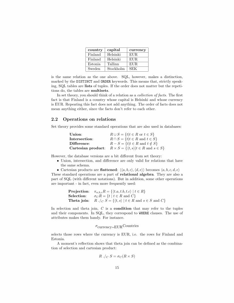
is the same relation as the one above. SQL, however, makes a distinction,marked by the DISTINCT and ORDER keywords. This means that, strictly speak-ing, SQL tables are lists of tuples. If the order does not matter but the repeti-tions do, the tables are multisets.
In set theory, you should think of a relation as a collection of facts. The firstfact is that Finland is a country whose capital is Helsinki and whose currencyis EUR. Repeating this fact does not add anything. The order of facts does notmean anything either, since the facts don’t refer to each other.
2.2 Operations on relations
Set theory provides some standard operations that are also used in databases:
Union: R ∪ S = t|t ∈ R or t ∈ SIntersection: R ∩ S = t|t ∈ R and t ∈ SDifference: R− S = t|t ∈ R and t /∈ SCartesian product: R× S = 〈t, s〉|t ∈ R and s ∈ S
However, the database versions are a bit different from set theory:• Union, intersection, and difference are only valid for relations that have
the same schema.• Cartesian products are flattened: 〈〈a, b, c〉, 〈d, e〉〉 becomes 〈a, b, c, d, e〉
These standard operations are a part of relational algebra. They are also apart of SQL (with different notations). But in addition, some other operationsare important - in fact, even more frequently used:
Projection: πa,b,cR = 〈t.a, t.b, t.c〉 | t ∈ RSelection: σCR = t | t ∈ R and CTheta join: R ./C S = 〈t, s〉 | t ∈ R and s ∈ S and C
In selection and theta join, C is a condition that may refer to the tuplesand their components. In SQL, they correspond to WHERE clauses. The use ofattributes makes them handy. For instance.
σcurrency=EURCountries
selects those rows where the currency is EUR, i.e. the rows for Finland andEstonia.
A moment’s reflection shows that theta join can be defined as the combina-tion of selection and cartesian product:
R ./C S = σC(R× S)
15

The ./ symbol without a condition denotes natural join, which joins tuplesthat have the same values of the common attributes. It used to be the basic formof join, but it is less common nowadays. Actually, maybe it should be avoidedbecause it relies on the names of attributes without making them explicit. Buthere is the definition if you want to see it:
R ./S= t+ 〈u.c1, . . . , u.ck〉|t ∈ R, u ∈ S, (∀a ∈ A ∩B)(t.a = u.a)
where A is the attribute set of R, B is the attribute set of S, and B − A =c1, . . . , ck. The + notation means putting together two tuples into one flat-tened tuple.
An alternative definition expresses natural join in terms of theta join (exer-cise!). Thus we can conclude: natural join is a special case of theta join, whichis a special case of the cartesian product. Projection is needed on top of this toremove the duplicate columns.
2.3 Multiple tables and joins
The joining operator supports dividing data to multiple tables. Consider thefollowing table:Countries:
name capital currency valueInUSDSweden Stockholm SEK 0.12Finland Helsinki EUR 1.09Estonia Tallinn EUR 1.09
This table has a redundancy, as the USD value of EUR is repeated twice.As we will see later, redundancy is usually avoided. For instance, someonemight update the USD value of the currency of Finland but forget Estonia,which would lead to inconsistency. You can also think of the database as astory that states some facts about the countries. Normally you would onlystate once the fact that EUR is 1.09 USD.
Redundancy can be avoided by splitting the table into two:JustCountries:
name capital currencySweden Stockholm SEKFinland Helsinki EUREstonia Tallinn EUR
Currencies:
code valueInUSDSEK 0.12EUR 1.09
16

Searching for the USD value of the currency of Sweden now involves a join ofthe two tables:
πvalueInUSD(JustCountries ./name=Sweden AND currency=code Currencies)
To anticipate Chapter 5, this is how it would be written in SQL:
SELECT valueInUSD
FROM JustCountries, Currencies
WHERE name = ’Sweden’ AND currency = code
Several things can be noted about this translation:• The SQL operator SELECT corresponds to projection in relation algebra,
not selection!• In SQL, WHERE corresponds to selection in relational algebra.• The FROM statement, listing any number of tables, actually forms their
cartesian product.Now, the SELECT-FROM-WHERE format is actually the most common idiomof SQL queries. As the FROM forms the cartesian product of potentially manytables, there is a risk that huge tables get constructed; keep in mind that thesize of a cartesian producs is the product of the sizes of its operand sets. Thequery compiler of the DBMS, however, can usually prevent this from happeningby query optimization. In this optimization, it performs a reduction of the SQLcode to something much simpler, typically equivalent to relational algebra code.
2.4 Referential constraints
The schemas of the two relations above are
JustCountries(country,capital,currency)
Currencies(code,valueInUSD)
For the integrity of the data, we want to require that all currencies in JustCountries
exist in Currencies. We add to the schema a referential constraint,
JustCountries(country,capital,currency)
currency -> Currencies.code
In the actual database, the referential constraint prevents us from inserting acurrency in JustCountries that does not exist in Currencies.
2.5 Key and uniqueness constraints
A key of a relation is an attribute that determines all other attributes. Acomposite key is a set of attributes that together determine all others. Wemark keys either by underlining or (in code ASCII text) with an underscoreprefix.
17

JustCountries(_name,capital,currency)
currency -> Currencies.code
Currencies(_code,valueInUSD)
In this example, name and code work naturally as keys. In JustCountries,capital could also work as a key, assuming that no two countries have the samecapital. This could be stated by adding one more statement to the schema, auniqueness constraint:
JustCountries(_name,capital,currency)
currency -> Currencies.code
unique capital
In the actual database, the key and uniqueness constraints prevent us frominserting a new country with the same name or capital.
In JustCountries, currency would not work as a key, because many coun-tries can have the same currency.
In Currencies, valueInUSD could work as a key, if it is unlike that twocurrencies have exactly the same value. This would not be very natural ofcourse. But the strongest reason of not using valueInUSD as a key is that weknow that some day two currencies might well get the same value.
A key can also be composite. This means that many attributes togetherform the key. For example, in
PostalCodes(_city,_street,code)
the city and the street together determine the postal code, but the city alone isnot enough. Nor is the street, because many cities may have the same street-name. For very long streets, we may have to look at the house number as well.The postal code determines the city but not the street. The code and the streettogether would be another possible composite key, but perhaps not very natural.
There is nothing that requires that all relations must have keys. Sometimesthis is even impossible, unless one includes all attributes in a composite key. Inmany databases, artificial keys are therefore created. For instance, Sweden hasintroduced a system of ”person numbers” to uniquely identify every resident ofthe country. Artificial keys may also be automatically generated by the systeminternally and never shown to the user. Then they are known as surrogatekeys.
2.6 Multiple values
The guiding principle of relational databases is that all types of the componentsare atomic. This means that they may not themselves be tuples. This is whatis guaranteed by the flattening of tuples of tuples in the relational version ofthe cartesian product. Another thing that is prohibited is list of values. Thinkabout, for instance, of a table listing the neighbours of each country. You mightbe tempted to write something like
18

country neighboursSweden Finland, NorwayFinland Sweden, Norway, Russia
But this is not possible, since the attributes cannot have list types. One has towrite a new line for each neighbourhood relationship:
country neighbourSweden FinlandSweden NorwayFinland SwedenFinland NorwayFinland Russia
The elimination of complex values (such as tuples and lists) is known as thefirst normal form, 1NF. It is nowadays built in in relational database systems,where it is impossible to define attributes with complex values.
2.7 Null values
Sometimes a value is unknown or known not to exist. The word NULL can thenbe used. Null values have no clear meaning in set theory. They should generallybe avoided, but may sometimes be handy as they simplify the schema.
19

3 Entity-Relationship diagrams
A popular device in modelling is E-R diagrams (Entity-Relationship diagrams).This chapter explains how different kinds of data are modelled by E-R diagrams.We will also tell how E-R diagrams can almost mechanically be derived from de-scriptive texts. Finally, we will explain how they are, even more mechanically,converted to relational schemes (and thereby eventually to SQL).
A relational database consists of a set of tables, which are linked to eachother by referential constraints. This is a simple model to implement and flexibleto use. But designing a database directly as tables can be hard, because onlysome things are ”naturally” tables; some other things are more like relationshipsbetween tables, and might seem to require a more complicated model.
E-R modelling is a richer structure than just tables, but it can be convertedto tables. Thus it helps design a database with right dependencies. When theE-R model is ready, it can be automatically converted to relational databaseschemas.
This chapter gives just the bare bones of E-R models. Their correct use isa skill that has to be practised. This practice is particularly suited for work inpairs: you should discuss the model with your lab partner. You should debate,challenge and disagree. Sometimes there are many models that are equallygood. But often a good-looking model is not so good if you take everything intoaccount. Four eyes see more than two.
The course book contains valuable examples and discussions. You can findsome more good examples in the old course slides. And of course, we will discussand give examples during the lecture!
Figure 2 shows an example of an E-R diagram. We will hopefully add someother examples in later versions of these notes.
3.1 E-R syntax
Standard E-R models have six kind of elements, each drawn with differentshapes:
entity rectangle a set of independent objectsrelationship diamond between 2 ore more entitiesattribute oval belongs to entity or relationshipISA relationship triangle between 2 entities, no attributesweak entity double-border rectangle depends on other entitiessupporting relationship double-border diamond between weak entity and its supporting entity
Between elements, there are connecting lines:• a relationship is connected to the entities that it relates• an attribute is connected to the entity or relationship to which it belongs• an ISA relationship is connected to the entities that it relates• a supporting relationship is connected to a weak entity and another (pos-
sibly weak) entity
20

Notice thus that there are no connecting lines directly between entities, or be-tween relationships, or from an attribute to more than one element. The ISArelationship has no attributes. It is just a way to indicate that one entity is asubentity of another one.
The connecting lines from a relationship to entities can have arrowheads:• sharp arrowhead: the relationship is to/from at most one object• round arrowhead: the relationship is to/from exactly one object• no arrowhead: the relationship is to/from many objectsThe attributes can be underlined or, equivalently, prefixed by . This means,
precisely as in relation schemas, that the attribute is a part of a key. The keysof E-R elements end up as keys and referential constraints of schemas.
Here is a simple grammar for defining E-R diagrams. It is in the ExtendedBNF format, where + means 1 or more repetitions, * means 0 or more, and ?
means 0 or 1.
Diagram ::= Element+
Element ::=
"ENTITY" Name Attributes
| "WEAK" "ENTITY" Name Support+ Attributes
| "ISA" Name SuperEntity Attributes
| "RELATIONSHIP" Name RelatedEntity+ Attributes
Attributes ::=
":" Attribute* # attributes start after colon
| # no attributes at all, no colon needed
RelatedEntity ::= Arrow Entity ("(" Role ")")? # optional role in parentheses
Support ::= Entity WeakRelationship
Arrow ::= "--" | "->" | "-)"
Attribute ::= Ident | "_"Ident
Entity, SuperEntity, Relationship, WeakRelationship, Role ::= Ident
This grammar is useful in two ways:• it defines exactly what combinations of elements are possible, so that you
can avoid ”syntax errors” (i.e. drawing impossible E-R diagrams)• it can be used as input to a program that draws the diagrams and converts
the model to a database schema (see below)Notice that there is no grammar rule for an Element that is a supporting re-lationship. This is because supporting relationships can only be introduced inthe Support part of weak entities.
3.2 From description to E-R
The starting point of an E-R diagram is often a text describing the domain. Youmay have to add your own understanding to the text. The expressions used in
21

the text may give clues to what kinds of elements to use. Here are some typicalexamples:
entity CN (common noun) ”country”attribute of entity the CN of X ”the population of X”attribute of relationship adverbial ”in 1995”relationship TV (transitive verb) ”X exports Y”relationship (more generally) sentence with holes ”X lies between Y and Z”subentity (ISA) modified CN ”EU country”weak entity CN of CN ”city of X”
It is not always the case that just these grammatical forms are used. You shouldrather try if they are usable as alternative ways to describe the domain. Forexample, when deciding if something is an attribute of an entity, you should tryif it really is the something of the entity, i.e. if it is unique. In this way, youcan decide that the population is an attribute of a country, but export productis not.
You can also reason in terms of the informal semantics of the elements:• An entity is an independent class of objects, which can have properties
(attributes) as well as relationships to other entities.• An attribute is a simple (atomic) property, such as name, size, colour,
date. It belongs to only one entity.• A relationship states a fact between two or more entities. These can also
be entities of the same kind (e.g. ”country X is a neighbour of countryY”).
• A subentity is a special case of a more general entity. It typically hasattributes that the general entity does not have. For instance, an EUcountry has the attribute ”joining year”.
• A weak entity is typically a part of some other entity. Its identity (i.e.key) needs this other entity to be complete. For instance, a city needs acountry, since ”Paris, France” is different from ”Paris, Texas”. The otherentity is called supporting entity, and the relationships are supportingrelationships. If the weak entity has its own key attributes, they arecalled discriminators (e.g. the name of the city).
3.3 Converting E-R diagrams to database schemas
The standard conversions are shown in Figure 1. The conversions are uniquefor ordinary entities, attributes, and many-to-many relationships.• An entity becomes a relation with its attributes and keys just as in E-R.• A relationship becomes a relation that has the key attributes of all related
entities, as well as its own attributes.Other kinds of elements have different possibilities:• In exactly-one relationships, one can leave out the relationship and use
the key of the related entity as attribute directly.
22

Figure 1: Translating E-R diagrams to database schemas. Picture by JonasAlmstrom-Duregard 2015.
23

• In weak entities, one likewise leaves out the relationship, as it is alwaysexactly-one to the strong entity.
• An at-most-one relationship can be treated in two ways:– the NULL approach: the same way as exactly-one, allowing NULL
values– the (pure) E-R approach: the same way as to-many, preserving the
relationship. No NULLs needed. However, the key of the relatedentity is not needed.
• An ISA relationship has three alternatives.– the NULL approach: just one table, with all attributes of all suben-
tities. NULLs are needed.– the OO (Object-Oriented) approach: separate tables for each suben-
tity and also for the superentity. No references between tables.– the E-R approach: separate tables for super-and subentity, subentity
refers to the superentity.As the name might suggest, the E-R approach is always recommended. It is themost flexible one, even though it requires more tables to be created.
One more thing: the naming of the tables of attributes.• Entity names could be turned from singular to plural nouns.• Attribute names must be made unique. (E.g. in a relationship from and
to the same entity).The course book actually uses plural nouns for entites, so that the conversionis easier. However, we have found it more intuitive to use singular nouns forentities, plural nouns for tables. The reason is that an entity is more like a kind(type), whereas a table is more like a list. The book uses the term entity setfor entities, which is the set of entities of the given kind.
3.4 Using the Query Converter*
Notice: The query converter is an experimental program that you might wantto try. It is in no way compulsory for the course. We will show a live demo atthe lecture. You can skip this section if you don’t want to try the program.
You can find the query converter (command qconv) in
https://github.com/GrammaticalFramework/gf-contrib/tree/master/query-converter/
You can specify an E-R model using the syntax described above. For example:
ENTITY Country : _name population
WEAK ENTITY City Country IsCityOf : _name population
ISA EUCountry Country : joiningDate
ENTITY Currency : _code name
RELATIONSHIP UsesAsCurrency -- Country -- Currency
If you have this text in the file countries.txt, then you can in qconv givethe command
24

Figure 2: An E-R diagram generated from the Query Converter qconv.
d countries.txt
The result is a diagram shown in Figure 2. You can see it if you have installedthe open-source Graphviz program. You will also get a database schema:
Country(_name,population)
City(_name,population,_name)
name -> Country.name
EUCountry(_name,joiningDate)
name -> Country.name
Currency(_code,name)
UsesAsCurrency(_countryName,_currencyCode)
countryName -> Country.name
currencyCode -> Currency.code
As an experimental feature, you will also get a text:
A country has a name and a population.
A city of a country has a name and a population.
25

Currencies(_code,name)
Ratings(_currencyCodeOf,_currencyCodeIn,_date,amount)
currencyCodeOf -> Currencies.code
currencyCodeIn -> Currencies.code
Figure 3: An E-R diagram for currency ratings, with two supporting relations,and the resulting schema.
An eucountry is a country that has a joining date.
A currency has a code and a name.
A country can use as currency a currency.
Figure 3 shows another example, where the weak entity Rating has twosupporting relations with Currency. This design was the result of a discussionat a lecture in 2016. It may look unusually complicated because of the weakentity with two supporting relationships. But the generated schema is entirelynatural, and we leave it as a challenge to obtain it from any other E-R design.
The Query Converter will be completed and improved during and after thecourse. It also has other functionalities: functional dependencies, normal forms,SQL, relational algebra.
26

4 Functional dependencies and normal forms
Mathematically, a relation can relate an object with many other objects. Forinstance, a country can have many neighbours. A function, on the other hand,relates each object with just one object. For instance, a country has just onenumber giving its area in square kilometres (at a given time). In this perspec-tive, relations are more general than functions. However, it is important toacknowledge that some relations are functions. Otherwise, there is a risk ofredundancy, repetition of the same information (in particular, of the sameargument-value pair). Redundancy can lead to inconsistency, if the informa-tion that should be the same in different places is actually not the same. Thiscan happen for instance as a result of updates, which is known as an updateanomaly. But functional dependencies can help prevent this from happening.They can be used for transforming the database into a normal form, whereredundancy is eliminated. There are many different normal forms, with weakeror stronger guarantees of consistency. This chapter will introduce three normalforms and two kinds of dependencies.
4.1 The design workflow
Functional dependency analysis is another tool for database design. It is quitedifferent from E-R diagrams and should ideally be used independently of it.One way to do this (common in textbook examples), is the following procedure:1. Collect all attributes into one and the same relation. At this point, it isenough to consider the relation as a set of attributes,
S = A1, . . . , An
2.Specify the functional dependencies and multivalued dependencies among theattributes. Informally,• a functional dependency (FD) A→ B means that, if you set the value
of A, there is only one possible value of B. This generalizes to sets ofattributes on both sides of the arrow.
• a multivalue dependency (MVD) A →→ B means that the value of Bdepends only on the value of A. But B can have many values for one andthe same value of A. This generalizes to sets of attributes on both sides ofthe arrow. The exact definition of MVD is a bit tricky, and MVD analysisis less common than FD analysis.
3. From the functional dependencies, calculate the possible keys of the relation.Informally,• a key is a combination X of attributes such that X → S, i.e. all attributes
of the relation are determined by the attributes in X.4. From the FDs, MVDs, and keys together, calculate the violations of normalforms. In summary,• violations of the third normal form (3NF) result from FDs• violations of the Boyce-Codd normal form (BCNF) likewise result from
FDs
27

• violations of the fourth normal form (4NF) result from MVDs5. From the normal form violations, compute a decomposition of the relationto a set of smaller relations. These smaller relations each have their own FDs,MVDs, and keys. But it is always possible to reach a state with no violationsby iterating the decomposition. The result is a set of tables, each with theirown keys, which have no violations.6. Decide what decomposition you want. All normal forms have their pros andcons. At this point, you may want to compare the dependency-based designwith the E-R design.
Dependency-based design is, in a way, more mechanical than E-R design.In E-R design, you have to decide many things: the ontological status of eachconcept (whether it is an entity, attribute, relationship, etc). You also have todecide the keys of the entities. In dependency analysis, you only have to decidethe basic dependencies. Lots of other dependencies are derived from these bymechanical rules. Also the possible keys - candidate keys - are mechanicallyderived. The decomposition to normal forms is mechanical as well. You justhave to decide what normal form (if any) you want to achieve. In addition, youhave to decide which of the candidate keys to declare as the primary key ofeach table.
4.2 Examples of dependencies and normal forms
4.2.1 Functional dependencies, keys, and superkeys
Let us start with a table of countries, currencies, and values of currencies (inUSD, on a certain day).
country currency valueSweden SEK 0.12Finland EUR 1.10Estonia EUR 1.10
We assume that each country has a unique currency, and each currency hasa unique value. This gives us two functional dependencies:
country -> currency
currency -> value
The dependencies are much like implications in the logical sense. Thus they aretransitive, which means that we can also infer the FD
country -> value
The set of attributes that can be inferred from a set of attributes X is theclosure of X. Thus, since value can be inferred from country, if belongs to itsclosure. In fact,
country+ = country, currency, value
28

noticing that A → A is always a valid FD, called trivial functional depen-dency.
Now, a possible key of a relation is a set of attributes whose closure is thewhole signature. Thus country alone is a possible key. However, it is not theonly set that determines all attributes. All of
country
country currency
country value
country currency value
do this. However, all of these sets but the first are just irrelevant extensions ofthe first. They are not keys but superkeys, i.e. supersets of keys. We concludethat country is the only possible key of the relation.
4.2.2 BCNF
What to do with the other functional dependency, currency -> value? Wecould call it a non-key FD, which is not standard terminology, but a handyterm. Looking at the table, we see that it creates a redundancy: the valueis repeated every time a currency occurs. Non-key FD’s are called BCNFviolations. They can be removed by BCNF decomposition: we build aseparate table for each such FD. Here is the result:
country currencySweden SEKFinland EUREstonia EUR
currency valueSEK 0.12EUR 1.10
These tables have no BCNF violations, and no redundancies either. Each ofthem has their own functional dependencies and keys:
Countries (_country, currency)
FD: country -> currency
reference: currency -> Currencies.currency
Currencies (_currency, value)
FD: currency -> value
They also enjoy lossless join: we can reconstruct the original table by a naturaljoin Countries ./ Currencies.
29

4.2.3 3NF
Now, let us consider an example where BCNF is not quite so beneficial. Hereis a table with cities, streets, and postal codes.
city street codeGothenburg Framnasgatan 41264Gothenburg Rannvagen 41296Gothenburg Horsalsvagen 41296Stockholm Barnhusgatan 11123
Here is the signature with functional dependencies:
city street code
city street -> code
code -> city
The keys are the composite keys city street and code street. But noticethat the non-key FD code -> city refers back to a key. If we now performBCNF decomposition, we obtain the schemas
Cities(_code, city)
FD: code -> city
Streets(_street, _code)
The problem with this decomposition is that we miss one FD, city street ->code. And in fact, the decomposition does not help remove redundancies. Theoriginal relation is fine as it is. It is already in the third normal form (3NF).3NF is like BCNF, except that a non-key FD X → A is allowed if A is a partof some key. Here, city is a part of a key, so it is fine. (An attribute that is apart of a key is called prime.)
Since the 3NF requirement is weaker than BCNF, it does not guarantee theremoval of all FD redundancies. But in many cases, the result is actually thesame: the country-currency-value table is an example.
4.2.4 4NF
Multivalued dependencies (MVD) are another kind of dependencies. AnMVD X →→ Y says that X determines Y independently of all other attributes.(The precise definition is a bit complicated, and is given in Section 4.3.)
Here is an example: a table of countries, their export products, and countriesthat they export to:
country product exportToSweden cars NorwaySweden paper DenmarkSweden cars DenmarkSweden paper Norway
30

In this table, Sweden exports both cars and paper to both Denmark and Norway.Now, let us assume it as a fact about the domain that, whatever a countryexports to some other country, it also exports to all other countries that it hastrade with. Then we have an MVD
country ->> product
Now, the table has a redundancy: both cars and paper and Norway and Den-mark are mentioned repeatedly. We can in fact find an 4NF violation: anMVD where the LHS is not a superkey. The 4NF decomposition splits thetable in accordance to the violating MVD:
country productSweden carsSweden paper
country exportToSweden NorwaySweden Denmark
These tables are free from violations. Hence they are in 4NF. Their naturaljoin losslessly returns the original table.
In the previous example, we could actually prove the MVD by looking at thetuples (see definition of MVD below). Finding a provable MVD in an instance ofa database can be difficult, because so many combinations must be present. AnMVD might of course be assumed to hold as a part of the domain description.This can lead to a better structure and smaller tables. However, the naturaljoin from those tables can produce combinations not existing in the reality.
4.2.5 A bigger example
Let us collect everything about a domain into one big table:
country capital popCountry popCapital currency value product exportTo
We identify some functional dependencies and multivalued dependencies:
country -> capital popCountry currency
capital -> country popCapital
currency -> value
country ->> product
One possible BCNF decomposition gives the following tables:
_country capital popCountry popCapital currency
_currency value
_country _product _exportTo
31

This looks like a good structure, except for the last table. Applying 4NF de-composition to this gives the final result
_country capital popCountry popCapital currency
_currency value
_country _product
_country _exportTo
A word of warning: mechanical decomposition can randomly choose some otherdependencies to split on, and lead to less natural results. For instance, it canuse capital rather than country as the key of the first table.
In the two sections that follow, we will show the precise algorithms that areinvolved, and which you should learn to execute by hand. The definitions mightlook more scary than they actually are. Most of the concepts are intuitivelysimple, but their precise definitions can require some details that one usuallydoesn’t think about. The notion of MVD is usually the most difficult one.
In the last section, we will look at the support given by the Query Converter(qconv) for dependency analysis and normal form decomposition.
4.2.6 One more example: FD or MVD?
(A similar example was treated with an MVD in the first version of these notes.But this turned out to be overkill: the same result can be achieved without theMVD.)
How should we model the neighbours of a country?
country population currency neighbour
We can assume that country determines the population and the currency. Hencethe FD
country -> population currency
But what about the neighbours? Surely a country can have many neighbours,so there is no FD here. But aren’t the neighbours independent of the populationand the currency? Then we would add the MVD
country ->> neighbour
However, recalling that (1) all FDs are are MVDs, and (2) MVDs are symmetric(see the definitions below), this MVD is actually a consequence of the FD! Henceadding it does not give anything new to our analysis.
In fact, the only key of the relation is country neighbour. This impliesthat the FD is a 3NF violation. Both 3NF and BCNF decomposition give thesame nice result:
country population currency
country neighbour
32

4.3 Mathematical definitions of dependencies
Before introducing new concepts, we will repeat some of the definitions abouttuples from Chapter 2. We will most of the time speak of relations just as theirsets of attributes. Also the dependency algorithms refer only to the attributes.But the definitions in the end do refer to tuples. By tuples, we will now meanlabelled tuples (records) rather than set-theoretic ordered tuples as in Chapter2.Definition (tuple, attribute, value). A tuple has the form
A1 = v1, . . . , An = vn
where A1, . . . , An are attributes and v1, . . . , vn are their values.Definition (signature, relation). The signature of a tuple, S, is the set ofall its attributes, A1, . . . , An. A relation R of signature S is a set of tupleswith signature S. But we will sometimes also say ”relation” when we mean thesignature itself.Definition (projection). If t is a tuple of a relation with signature S, theprojection t.Ai computes to the value vi.Definition (simultaneous projection). If X is a set of attributes B1, . . . , Bm ⊆S and t is a tuple of a relation with signature S, we can form a simultaneousprojection,
t.X = B1 = t.B1, . . . , Bm = t.Bm
Definition (functional dependency, FD). Assume X is a set of attributes and Aan attribute, all belonging to a signature S. Then A is functionally dependenton X in the relation R, written X → A, if• for all tuples t,u in R, if t.X = u.X then t.A = u.A.
If Y is a set of attributes, we write X → Y to mean that X → A for every Ain Y.Definition (multivalued dependency, MVD). Let X,Y,Z be disjoint subsets of asignature S such that S = X∪Y ∪Z. Then Y has a multivalued dependencyon X in R, written X →→ Y , if• for all tuples t,u in R, if t.X = u.X then there is a tuple v in R such that
– v.X = t.X– v.Y = t.Y– v.Z = u.Z
An alternative notation is X →→ Y | Z, emphasizing that Y is independentof Z.
To see the power of these definitions, we can now easily prove a slightlysurprising result saying that every FD is an MVD:Theorem. If X → Y then X →→ YProof. Assume that t,u are tuples in R such that t.X = u.X. We select v = u.This is a good choice, because
1 u.X = t.X by assumption2 u.Y = t.Y by the functional dependency X → Y3 u.Z = u.Z by reflexivity of identity.
33

Note. MVDs are symmetric on their right hand side: if X →→ Y , which meansX →→ Y | Z where Z = S −X − Y , then also X →→ Z. Thus in the example inSection 4.2.4, we could have written, equivalently,
country ->> exportedTo
4.4 Definitions of closures, keys, and superkeys
As a starting point of dependency analysis, a relation is charaterized by itssignature S, its functional dependencies FD, and its multivalued dependenciesMVD. We start with things where we don’t need MVD.Assume thus a signature (i.e. set of attributes) S and a set FD of functionaldependencies.Definition. An attribute A follows from a set of attributes Y, if there is anFD X → A such that X ⊆ Y .Definition (closure of a set of attributes under FDs). The closure of a set ofattributes X ⊆ S under a set FD of functional dependencies, denoted X+, isthe set of those attributes that follow from X.Algorithm (closure of attributes). If X ⊆ S, then the closure X+, can becomputed in the following way:
1. Start with X+ = X2. Set New = A | A ∈ S,A /∈ X+, A follows from X+3. If New = ∅, return X+, else set X+ = X + ∪New and go to 1
Definition (closure of a set of FDs). The closure of a set FD of functionaldependencies, denoted by FD+, is defined as follows:
FD+ = X → A | X ⊆ S,A ∈ X+, A /∈ X
The last condition excludes trivial functional dependencies.Definition (trivial functional dependencies). An FD X → A is trivial, ifA ∈ X.Definition (superkey, key). A set of attributes X ⊆ S is a superkey of S, ifS ⊆ X+.A set of attributes X ⊆ S is a key of S if• X is a superkey of S• no proper subset of X is a superkey of S
4.5 Definitions and algorithms for normal forms
Definition (Boyce-Codd Normal Form, BCNF violation). A functional depen-dency X → A violates BCNF if• X is not a superkey• the dependency is not trivial
A relation is in Boyce-Codd Normal Form (BCNF) if it has no BCNFviolations.Note. Any trivial dependency A→ A always holds even if A is not a superkey.Definition (prime). An attribute A is prime if it belongs to some key.
34

Definition (Third Normal Form, 3NF violation). A functional dependencyX → A violates 3NF if• X is not a superkey• the dependency is not trivial• A is not prime
Note. 3NF is a weaker normal form than BCNF: Any violation X → A of 3NFis also a violation of BCNF, because it says that X is not a superkey. Hence,any relation that is in BCNF is also in 3NF.Definition (trivial multivalued dependency). A multivalued dependencyX →→ Ais trivial if Y ⊆ X or X ∪ Y = S.Definition (Fourth Normal Form, 4NF violation). A multivalued dependencyX →→ A violates 4NF if• X is not a superkey• the MVD is not trivial.
Note. 4NF is a stronger normal form than BCNF: If X → A violates BCNF,then it also violates 4NF, because• it is an MVD by the theorem above• it is not trivial, because
– if A ⊆ X, then X → A is a trivial FD and cannot violate BCNF– if X ∪ A = S, then X is a superkey and X → A cannot violate
BCNFAlgorithm (BCNF decomposition). Consider a relation R with signature Sand a set F of functional dependencies. R can be brought to BCNF by thefollowing steps:
1. If R has no BCNF violations, return R2. If R has a violating functional dependency X → A, decompose R to two
relations
• R1 with signature X ∪ A• R2 with signature S − A
3. Apply the above steps to R1 and R2 with functional dependencies pro-jected to the attributes contained in each of them.
One can combine several violations with the same left-hand-side X to producefewer tables. Then the violation X → Y decomposes R to R1(X,Y ) and R2(S−Y ).Note. Step 3 of the BCNF decomposition algorithm involves the projectionof functional dependencies. This can in general be a complex procedure.However, for most cases handled during this course, it is enough just to filterout those dependencies that do not appear in the new relations.Algorithm (4NF decomposition). Consider a relation R with signature S anda set M of multivalued dependencies. R can be brought to 4NF by the followingsteps:
1. If R has no 4NF violations, return R2. If R has a violating multivalued dependency X →→ Y , decompose R to
two relations
35

• R1 with signature X ∪ Y • R2 with signature S − Y
3. Apply the above steps to R1 and R2Note. This algorithm has the same structure as the BCNF decomposition.For 3NF decomposition, a very different algorithm is used, seemingly with noiteration. But an iteration can be needed to compute the minimal basis of theFD set.Concept (minimal basis of a set of functional dependencies; not a rigorousdefinition). A minimal basis of a set F of functional dependencies is a set F-that implies all dependencies in F. It is obtained by first weakening the left handsides and then dropping out dependencies that follow by transitivity. Weakeningan LHS in X → A means finding a minimal subset of X such that A can stillbe derived from F-.Algorithm (3NF decomposition). Consider a relation R with a set F of func-tional dependencies.
1. If R has no 3NF violations, return R.2. If R has 3NF violations,
• compute a minimal basis of F- of F• group F- by the left hand side, i.e. so that all depenencies X → A
are grouped together• for each of the groups, return the schema XA1 . . . An with the com-
mon LHS and all the RHSs• if one of the schemas contains a key of R, these groups are enough;
otherwise, add a schema containing just some keyExample (minimal basis). Consider the schema
country currency value
country -> currency
country -> value
currency -> value
It has one 3NF violation: currency -> value. Moreover, the FD set is not aminimal basis: the second FD can be dropped because it follows from the firstand the third ones by transitivity. Hence we have a minimal basis
country -> currency
currency -> value
Applying 3NF decomposition to this gives us two schemas:
country currency
currency value
i.e. exactly the same ones as we would obtain by BCNF decomposition. Theserelations are hence not only 3NF but also BCNF.
36

4.6 Relation analysis in the Query Converter*
The qconv command f reads a relation from a file and prints out relation info:• the closure of functional dependencies• superkeys• keys• normal form violations
The command n reads a relation from the same file format and prints out de-compositions in 3NF, BCNF, and 4NF.
The format of these files is as in the following example:
country capital popCountry popCapital currency value product exportTo
country -> capital popCountry currency
capital -> popCapital
currency -> value
country ->> product
The Haskell code in
https://github.com/GrammaticalFramework/gf-contrib/blob/master/query-converter/Fundep.hs
is a direct rendering of the mathematical definitions. There is a lot of room foroptimizations, but as long as the number of attributes is within the usual limitsof textbook exercises, the naive algorithms work perfectly well.
4.7 Further reading on normal forms and functional de-pendencies*
The following is a practical guide going through all the normal forms from 1NFto 5NF:
William Kent, ”A Simple Guide to Five Normal Forms in RelationalDatabase Theory”, Communications of the ACM 26(2), Feb. 1983,120-125. http://www.bkent.net/Doc/simple5.htm
37

5 SQL
Here we start getting our hands dirty with SQL. This chapter covers two lec-tures. At the first lacture, we will explain the main language constructs of SQL.We will turn database schemas to SQL definitions. We will build a database byinsertions. We will query it by selections, projections, joins, renamings, unions,intersections, etc. At the second lecture, we add SQL groupings and aggrega-tions, as well as views. We will also take a look at low-level manipulations ofstrings and at the different datatypes of SQL.NOTE: This chapter is not an SQL tutorial, but an overview of the syntax andsemantics of the language. We do give some examples of SQL usage, but focusmore on possibly surprising things than the common usage. The book givesmany more examples, and there is a detailed on-line tutorial in
http://www.w3schools.com/sql/
This tutorial also has a nice index of SQL keywords.
5.1 SQL in a nutshell
Figure 4 shows a grammar of SQL. It is not full SQL, but it does contain all thoseconstructs that are used in this course for database definitions and queries. Thesyntax for triggers, indexes, authorizations, and transactions will be covered inlater chapters.
In addition to the standard constructs, different DBMSs contain their ownones, thus creating ”dialects” of SQL. They may even omit some standard con-structs. In this respect, PostgreSQL is closer to the standard than many othersystems.
The grammar notation aimed for human readers. It is hence not completelyformal. A full formal grammar can be found e.g. in PostgreSQL references:
http://www.postgresql.org/docs/9.5/interactive/index.html
Another place to look is the Query Converter source file
https://github.com/GrammaticalFramework/gf-contrib/blob/master/query-converter/MinSQL.bnf
It is roughly equivalent to Figure 4, and hence incomplete. But it is completelyformal and is used for implementing an SQL parser.1
The grammar is BNF (Backus Naur form) with the following conventions:• CAPITAL words are SQL keywords, to take literally• small character words are names of syntactic categories, defined each in
their own rules• | separates alternatives
1 The parser is generated by using the BNF Converter tool,http://bnfc.digitalgrammars.com/ which is also used for the relational algebra andXML parsers in qconv.
38

statement ::= type ::=
CREATE TABLE tablename ( CHAR ( integer ) | VARCHAR ( integer ) | TEXT
* attribute type inlineconstraint* | INT | FLOAT
* [CONSTRAINT name]? constraint
) ; inlineconstraint ::= ## not separated by commas!
| PRIMARY KEY
DROP TABLE tablename ; | REFERENCES tablename ( attribute ) policy*
| | UNIQUE | NOT NULL
INSERT INTO tablename tableplaces? values ; | CHECK ( condition )
| | DEFAULT value
DELETE FROM tablename
? WHERE condition ; constraint ::=
| PRIMARY KEY ( attribute+ )
UPDATE tablename | FOREIGN KEY ( attribute+ )
SET setting+ REFERENCES tablename ( attribute+ ) policy*
? WHERE condition ; | UNIQUE ( attribute+ ) | NOT NULL ( attribute )
| | CHECK ( condition )
query ;
| policy ::=
CREATE VIEW viewname ON DELETE|UPDATE CASCADE|SET NULL
AS ( query ) ; ## alternatives: CASCADE and SET NULL
|
ALTER TABLE tablename tableplaces ::=
+ alteration ; ( attribute+ )
|
COPY tablename FROM filepath ; values ::=
## postgresql-specific, tab-separated VALUES ( value+ ) ## keyword VALUES only in INSERT
| ( query )
query ::=
SELECT DISTINCT? columns setting ::=
? FROM table+ attribute = value
? WHERE condition
? GROUP BY attribute+ alteration ::=
? HAVING condition ADD COLUMN attribute type inlineconstraint*
? ORDER BY attributeorder+ | DROP COLUMN attribute
|
query setoperation query localdef ::=
| WITH tablename AS ( query )
query ORDER BY attributeorder+
## no previous ORDER in query columns ::=
| "*"
WITH localdef+ query | column+
table ::= column ::=
tablename expression
| table AS? tablename ## only one iteration allowed | expression AS name
| ( query ) AS? tablename
| table jointype JOIN table ON condition attributeorder ::=
| table jointype JOIN table USING (attribute+) attribute (DESC|ASC)?
| table NATURAL jointype JOIN table
setoperation ::=
condition ::= UNION | INTERSECT | EXCEPT
expression comparison compared
| expression NOT? BETWEEN expression AND expression jointype ::=
| condition boolean condition LEFT|RIGHT|FULL OUTER?
| expression NOT? LIKE ’pattern*’ | INNER?
| expression NOT? IN values
| NOT? EXISTS ( query ) comparison ::=
| expression IS NOT? NULL = | < | > | <> | <= | >=
| NOT ( condition )
compared ::=
expression ::= expression
attribute | ALL|ANY values
| tablename.attribute
| value operation ::=
| expression operation expression "+" | "-" | "*" | "/" | "%"
| aggregation ( DISTINCT? *|attribute) | "||"
| ( query )
pattern ::=
value ::= % | _ | character ## match any string/char
integer | float | ’string’ | [ character* ]
| value operation value | [^ character* ]
| NULL
aggregation ::=
boolean ::= MAX | MIN | AVG | COUNT | SUM
AND | OR
Figure 4: A grammar of the main SQL constructs.
39

• + means one or more, separated by commas• * means zero or more, separated by commas• ? means zero or one• in the beginning of a line, + * ? operate on the whole line; elsewhere,
they operate on the word just before• ## start comments, which explain unexpected notation or behaviour• text in double quotes means literal code, e.g. "*" means the operator *• other symbols, e.g. parentheses, also mean literal code (quotes are used
only in some cases, to separate code from grammar notation)• parentheses can be added to disambiguate the scopes of operators
Another important aspect of SQL syntax is case insensitivity:• keywords are usually written with capitals, but can be written by any
combinations of capital and small letters• the same concerns identifiers, i.e. names of tables, attributes, constraints• however, string literals in single quotes are case sensitive
5.2 Database and table definitions
Logically, the creation of a database starts with a statement
CREATE DATABASE dbname ;
But you will seldom see this statement. If you use the school’s PostgreSQLinstallation, you already have a database created, and you should work underthat. If you are administrating your own PostgreSQL installation, you may usethe Unix shell command
createdb dbname
After this, you can start PostgreSQL with the Unix shell command
psql dbname
Once a database is created, tables can be added by CREATE TABLE state-ments. These statements implement the database schemas as discussed in earlierchapters. Unlike in schemas, types are compulsory, but keys are not.
This leads us to a translation from relation schemas to SQL statements. Thegeneral form of a schema is
relation ( attribute , ... , attribute )
foreignAttribute -> relation.attribute
...
foreignAttribute -> relation.attribute
This is converted to the SQL statemant
40

CREATE TABLE relation (
attribute type,
...
attribute type,
PRIMARY KEY ( keyAttributes ),
FOREIGN KEY ( foreignAttribute ) REFERENCES relation (attribute),
...
FOREIGN KEY ( foreignAttribute ) REFERENCES relation (attribute)
)
where each type is selected in a suitable way. The ”primary key” can be a tupleof attributes. The ”foreign keys” can also be grouped into tuples.
As for the types, SQL has several types for strings: CHAR(n), VARCHAR(n),and TEXT. In earlier times, and in other DBMSs, these types may have perfor-mance errors. However, the PostgreSQL manual says as follows: ”There are noperformance differences between these types... In most situations text or char-acter varying (= varchar) should be used.” Following this advice, we will in thefollowing use TEXT as the only string type. Objects of all the three types arestring literals in single quotes (e.g. ’foo bar’). Spaces are preserved.
Example:
Countries (_name,capital,population,currency)
capital -> Cities.name
currency -> Currencies.code
gives
CREATE TABLE Countries (
name TEXT,
capital TEXT,
population INT,
currency TEXT,
PRIMARY KEY (name),
FOREIGN KEY (capital) REFERENCES Cities (name),
FOREIGN KEY (currency) REFERENCES Currencies (code)
)
In addition to these schema elements, some other constraints can be added. Forexample, in this case, the following would make sense:
UNIQUE (capital),
NOT NULL (capital)
as a way to express that capital is another candidate key of Countries. This istold us by the functional dependencies, but only one set of attributes can bethe PRIMARY KEY. Notice that UNIQUE, unlike PRIMARY KEY, does notimply NOT NULL, so this must be stated separately.
Constraints can also be given names:
41

CONSTRAINT primaryKeyName PRIMARY KEY (name)
This may help get better error messages. It also makes it possible to removeconstraints later if needed. At the opposite end of verbosity are inline con-straints, which are stated together with the attributes they concern:
name TEXT PRIMARY KEY
More on constraints will follow in Chapter 6, where in particular the CHECKconstraints are discussed.
5.3 Inserting values
The INSERT INTO statement works with both value lists and queries. Here isa list:
INSERT INTO Places VALUES (’Oslo’,’Norway’,’60N’)
where the fields must match the schema of Places; we could here assume
Places (name TEXT, country TEXT, latitude TEXT)
If we want to quickly populate Places by the capitals of countries, we can do
INSERT INTO Places (SELECT capital,name FROM Countries)
This will leave the latitude attribute undefined. Alternatively, we can initializethe latitude with a value, e.g. ’0’ (because this is the longest latitude on theglobe and therefore the most probable choice ;-):
INSERT INTO Places (SELECT capital,name,’0’ FROM Countries)
As yet another alternative, the CREATE TABLE statement could have specifieda default for latitude with an inline constraint,
latitude TEXT DEFAULT ’0’
There are always many ways of expressing the things in SQL! (However, DE-FAULT constraints cannot appear separately in the usual way but must beinlined.)
In PostgreSQL, there is a quick way to insert values from tab-separated files:
COPY tablename FROM filepath
Notice that a complete filepath is required. The data in the file must of coursematch your database schema. To give an example, if you have a table
Countries (name,capital,area,population,continent,currencycode,currencyname)
you can read data from a file that looks like this:
42

Andorra Andorra la Vella 468 84000 EU EUR Euro
United Arab Emirates Abu Dhabi 82880 4975593 AS AED Dirham
Afghanistan Kabul 647500 29121286 AS AFN Afghani
The file
https://github.com/GrammaticalFramework/gf-contrib/blob/master/query-converter/countries.tsv
can be used for this purpose. It is extracted from the Geonames database,http://www.geonames.org/
An alternative method is to generate lots of INSERT commands into a file.Such a file can also include other SQL commands - you can, for instance, saveall your work in it. Then you can build your database, or parts of it, with thePostgreSQL command
\i file.sql
5.4 Query usage and semantics: simple queries
This section covers the part of SQL presented on Lecture 5.The most common form of a query is
SELECT attributes
FROM tables
WHERE condition
It corresponds to the relational algebra expression
πattributesσcondition(table× . . .× table)
Thus, to understand its meaning, it should be read in the order in which theprocessing happens:
FROM tables WHERE condition SELECT attributes
Notice that only the SELECT part is compulsory; you can use it on an expres-sion that doesn’t refer to any table:
SELECT 2+2
5.4.1 The cartesian product (FROM)
Here we list the table names we want to query about. If the same table is usedtwice, it can be given different names:
SELECT A.name, B.capital
FROM Countries AS A, Countries AS B
WHERE A.name = B.capital
43

shows countries that have the same name as some country’s capital.A table can also be given as a subquery. In this case, it is obligatory to give
it a name.
SELECT name
FROM (
SELECT name,capital
FROM countries) AS C
WHERE C.name = C.capital
shows countries that have the same name as their capital. (The subquery israther superfluous in this very example, though.)
In addition to table names and subqueries, tables formed by different JOINoperations can be included. More on this in Section 5.5.4.
5.4.2 The condition on attributes (WHERE)
Conditions are boolean-valued expressions. The WHERE clause filters thosetuples that make the condition TRUE. The conditions are built by• comparison operators (such as =, <, <>, (NOT) LIKE) from expres-
sions referring values in tuples– a special kind of comparison is with ALL and ANY, compared to a
list of values or a subquery.x < ALL (2,3,4)
means that x is at most 1. If we change ALL to ANY, then x mustbe at most 3.
• query-related operators (NOT) EXISTS and (NOT) IN from subqueries• logical operators (AND, OR, NOT) from conditions
The operand expressions can be
• literals (strings, integers, floats)
• attributes, possibly qualified with table names
• built from other expressions with arithmetic operations (+, -, etc)
• subqueries returning exactly one atomic values, e.g.
(SELECT capital FROM Countries WHERE name = ’Sweden’)
More precisely, conditions have a three-valued logic, because of the pres-ence of NULL. Comparisons with NULL always result in UNKNOWN.Logical operators have the following meanings (T = TRUE, F = FALSE,U = UNKNOWN)
44
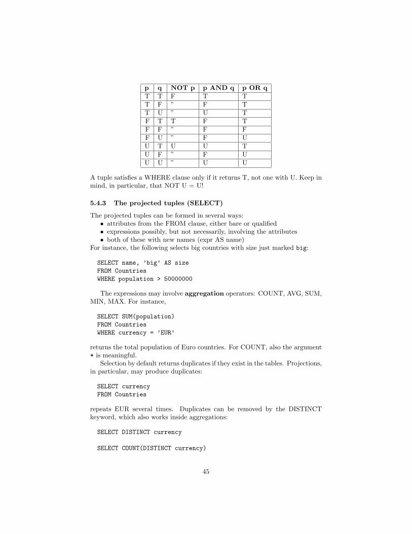
p q NOT p p AND q p OR qT T F T TT F ” F TT U ” U TF T T F TF F ” F FF U ” F UU T U U TU F ” F UU U ” U U
A tuple satisfies a WHERE clause only if it returns T, not one with U. Keep inmind, in particular, that NOT U = U!
5.4.3 The projected tuples (SELECT)
The projected tuples can be formed in several ways:• attributes from the FROM clause, either bare or qualified• expressions possibly, but not necessarily, involving the attributes• both of these with new names (expr AS name)
For instance, the following selects big countries with size just marked big:
SELECT name, ’big’ AS size
FROM Countries
WHERE population > 50000000
The expressions may involve aggregation operators: COUNT, AVG, SUM,MIN, MAX. For instance,
SELECT SUM(population)
FROM Countries
WHERE currency = ’EUR’
returns the total population of Euro countries. For COUNT, also the argument* is meaningful.
Selection by default returns duplicates if they exist in the tables. Projections,in particular, may produce duplicates:
SELECT currency
FROM Countries
repeats EUR several times. Duplicates can be removed by the DISTINCTkeyword, which also works inside aggregations:
SELECT DISTINCT currency
SELECT COUNT(DISTINCT currency)
45

5.4.4 Set operations on queries (UNION, INTERSECT, EXCEPT)
Set operations can be applied to queries, even on the top level. Thus
SELECT name, ’big’ AS size FROM countries WHERE population >= 50000000
UNION
SELECT name, ’small’ AS size FROM countries WHERE population < 50000000
shows the populations of countries just as big or small.UNION, INTERSECT, EXCEPT correspond to the set operations ∪,∩,−
introduced in Chapter 2. Thus they can only be applied to tables ”of the sametype”, i.e. tuples with the same number of elements of the compatible types.The attribute names, however, need not match: it is meaningful to write
SELECT capital FROM Countries
UNION
SELECT name FROM Countries
5.5 Query usage and semantics: more complex queries
This section covers the part of SQL presented on Lecture 6.The full form of SELECT queries is, as specified in the grammar,
WITH localdefinitions -- give names to auxiliary queries
SELECT attributes
FROM tables
WHERE condition
GROUP BY attributes -- divide the table to groups
HAVING condition -- conditions on the groups
ORDER BY attributes -- order the table in a desired way
5.5.1 Local definitions (WITH)
Local definitions (WITH clauses) are a simple shorthand mechanism forqueries. Thus
WITH
EuroCountries AS (
SELECT *
FROM countries
WHERE currency = ’EuroCountries’
)
SELECT *
FROM EuroCountries A, EuroCountries B
WHERE ...
is a way to avoid the duplication of the query selecting the countries using theEuro as their currency.
46

5.5.2 Sorting (ORDER BY)
Sorting (ORDER BY) lists a set of attributes considered in lexicographicalorder. The direction of sorting can be specified for each attribute as DESCor ASC, where ASC is the default. Thus the following query sorts countriesprimarily by the currency in ascending order, secondarily by size in descendingorder:
SELECT currency, name, population
FROM Countries
ORDER BY currency, population DESC
ORDER BY is usually presented as a last field of a SELECT group. But it canalso be appended to a query formed by a set-theoretic operation:
(SELECT name, ’big’ AS size FROM countries WHERE population >= 50000000
UNION
SELECT name, ’small’ AS size FROM countries WHERE population >= 50000000
) ORDER BY size, name
shows first all big countries in alphabetical order, then all small ones.
5.5.3 Grouping (GROUP BY) and group conditions (HAVING)
Applying GROUP BY a to a table R forms a new table, where a is the key.For instance, GROUP BY currency forms a table of currencies. But what are theother attributes? The original attributes of R won’t do, because each of themmay appear many times. For instance, there are many EUR countries. So whatis the use of this construction?
The full truth about GROUP BY can be seen only by looking at the SELECTline above it. On this line, only the following attributes of R may appear:• the grouping attribute a itself• aggregation functions on the other attributes
In other words, the new relation has these aggregation functions as its non-keyattributes. Here is an example:
SELECT currency, COUNT(name)
FROM Countries
GROUP BY currency
currency | count
----------+-------
XCD | 8
ETB | 1
HUF | 1
...
47

Now, most rows in this table will have count 1. We may be interested on onlythose currencies that are used by more than one country. The standard way ofdoing this is by a subquery:
SELECT *
FROM (
SELECT currency, COUNT(name) AS number
FROM Countries
GROUP BY currency) AS C
WHERE number > 1
This shows clearly that GROUP BY really forms a table. But SQL also providesa shorthand way of expressing conditions on the groups (i.e. the rows of therelation formed by GROUP BY): HAVING:
SELECT currency, COUNT(name)
FROM Countries
GROUP BY currency
HAVING COUNT(name) > 1
If you want to order this from the biggest to the smallest count, just add theline
ORDER BY COUNT(name) DESC
currency | count
----------+-------
EUR | 35
USD | 17
XOF | 8
...
The other aggregation functions (SUM, AVG, MAX, MIN) work in the sameway. The grouped table can have more than one of them:
SELECT currency, COUNT(name), AVG(population)
FROM countries
GROUP BY currency
As a final subtlety: the relation formed by GROUP BY also contains the ag-gregations used in the HAVING clause or the ORDER BY clause:
SELECT currency, AVG(population)
FROM Countries
GROUP BY currency
HAVING COUNT(name) > 1
SELECT currency, AVG(population)
48
FROM Countries
GROUP BY currency
ORDER BY COUNT(name) DESC
From the semantic point of view, GROUP BY is thus a very complex operator,because one has to look at many different places to see exactly what relation itforms. We will get more clear about this when looking at relational algebra andquery compilation in Chapter 7.
5.5.4 Join operations (JOIN)
The syntax of join operations is rich, as there are 24 different join operations:
table ::= -- 24 = 8+8+8
tablename
| table jointype JOIN table ON condition -- 8
| table jointype JOIN table USING (attribute+) -- 8
| table NATURAL jointype JOIN table -- 8
jointype ::= -- 8 = 6+2
LEFT|RIGHT|FULL OUTER? -- 6 = 3*2
| INNER? -- 2
In addition, cartesian product itself is a kind of a join. It is also called CROSSJOIN, but we will use the ordinary notation with commas instead.
Luckily, the JOINs have a compositional meaning. INNER is the simplestjoin type, and the keyword can be omitted without change of meaning. ThisJOIN with the ON condition gives the purest form of theta join:
FROM table JOIN table ON condition
is equivalent to
FROM table,table
WHERE condition
The condition is typically looking for attributes with equal values in the twotables. With good luck (or design) such attributes have the same name, andone can write
L JOIN R USING (a,b)
as a shorthand for
L JOIN R ON L.a = R.a AND L.b = R.b
well... almost, since when JOIN is used with ON, it repeats the values of a anb from both tables, like cartesian product does.
An extreme case is NATURAL JOIN, where no conditions are needed. It isequivalent to
49

L JOIN R USING (a,b,c,...)
which lists all common attributes of L and R.Cross join, inner joins, and natural join only include tuples where the join
attribute exists in both tables. Outer joins can fill up from either side. Thusleft outer join includes all tuples from L, right outer join from R, and full outerjoins from both L and R.
Here are some examples of inner and outer joins:
L
a | b
----+----
11 | 21
12 | 22
R
a | c
----+----
12 | 32
13 | 33
L cross join R
a | b | a | c
----+----+----+----
11 | 21 | 12 | 32
11 | 21 | 13 | 33
12 | 22 | 12 | 32
12 | 22 | 13 | 33
L inner join R on L.a = R.a ;
a | b | a | c
----+----+----+----
12 | 22 | 12 | 32
L natural join R
a | b | c
----+----+----
12 | 22 | 32
L inner join R using (a)
a | b | c
----+----+----
12 | 22 | 32
L full outer join R using (a)
a | b | c
50

----+----+----
11 | 21 |
12 | 22 | 32
13 | | 33
L left outer join R using (a)
a | b | c
----+----+----
11 | 21 |
12 | 22 | 32
L right outer join R using (a)
a | b | c
----+----+----
12 | 22 | 32
13 | | 33
5.5.5 Pattern matching (LIKE)
The condition s LIKE p compares the string s with the pattern p. The patterncan use wildcards (for any character) and % (for any substring). Thus
WHERE name LIKE ’%en’
is satisfied by all countries whose name ends with ”en”, e.g. Sweden.
5.6 Views (CREATE VIEW)
A view is like a constant defined in a WITH clause, but its definition is global.Views are used for ”frequently asked queries”. They are built each time fromthe underlying tables, and hence redundancy is not an issue.
5.7 SQL pitfalls
Here we list some things that do not feel quite logical in SQL design, or whosesemantics may feel surprising.
Tables vs. queries
In relational algebra, a query is always an expression for a table (i.e. relation).In SQL, however, there are subtle syntax differences:• A bare table name is not a valid query. A bare FROM part is not
a valid query either. The shortest way to list all tuples of a table isSELECT * FROM table
• Set operations can only combine queries, not table names.• Join operations can only combine table names, not queries.
51

• A cartesian product in a FROM clause can mix queries and table names,but...
• When a query is used in a FROM clause, it must be given an AS name.• A WITH clause can only define constants for queries, not for table expres-
sions.
Renaming syntax
Renaming is made with the AS operator, which however has slightly differentuses:• In WITH clauses, the name is before the definition: name AS (query).• In SELECT parts, the name is after the definition: expression AS name.• In FROM parts, the name is after the definition but AS may be omitted:table AS? name.
Cartesian products
The bare cartesian product from a FROM clause can be a huge table, sincethe sizes are multiplied. With the same logic, if the product contains an emptytable, its size is 0 as well. Then it does not matter that the empty table mightbe ”irrelevant”:
SELECT A.a FROM A, Empty
results in an empty table.
NULL values and three-valued logic
Because of NULL values, SQL follows a three-valued logic: TRUE, FALSE,UNKNOWN. The truth tables as such are natural. But the way they are usedin e.g WHERE clauses is good to keep in mind. Recalling that a comparisonwith NULL results in UNKNOWN, and that WHERE clauses only select TRUEinstances, the query
SELECT ...
FROM ...
WHERE v = v
gives no results for tuples where v is NULL. The same concerns
SELECT ...
FROM ...
WHERE v < 10 OR v >= 10
Hence if v is NULL, it cannot even be assumed that it has the same value in alloccurrences.
Another example, given in
52

https://www.simple-talk.com/sql/t-sql-programming/ten-common-sql-programming-mistakes/
as the first one among the ”Ten common SQL mistakes”, involves NOT IN:since
u NOT IN (1,2,v)
means
NOT (u = 1 OR u = 2 OR u = v)
this evaluates to UNKNOWN if v is NULL. Hence it can be useless as a test.
Set operations are set operations
Being a set means that duplicates don’t count. This is what holds of relationalalgebra, but SQL is usually about multisets, so that duplicates do count. How-ever, the set operations UNION, INTERSECT, EXCEPT do remove duplicates!Hence
SELECT * FROM table
UNION
SELECT * FROM table
has the same effect as
SELECT DISTINCT * FROM table
5.8 SQL in the Query Converter*
The Query Converter has an SQL parser and interpreter, which works much thesame way as the PostgreSQL shell. Thus you can give SQL commands in theqconv shell, and the database is queried and updated accordingly. You can alsosee the relational algebra translations of your queries. This is in fact the onlyreason to use qconv as an SQL interpreter rather than PostgreSQL.
Only a part of SQL is currently recognized by qconv. The interpreter maymoreover be buggy. The database is only built in memory, not stored on a disk.Thus you should store your work in an SQL source file. Such files can be readwith the i (”import”) command, for instance,
> i countries.sql
which uses the file
https://github.com/GrammaticalFramework/gf-contrib/blob/master/query-converter/countries.sql
53

6 Table modification and triggers
Here we take a deeper look at inserts, updates, and deletions, in the presence ofconstraints. The integrity constraints of the database may restrict these actionsor even prohibit them. An important problem is that when one piece of datais changed, some others may need to be changed as well. For instance, whena row is deleted or updated, how should this affect other rows that reference itas foreign key? Some of these things can be guaranteed by constraints in basicSQL. But some things need more expressive power. For example, when makinga bank transfer, money should not only be taken from one account, but the sameamount must be added to the other account. For situations like this, DBMSssupport triggers, which are programs that do many SQL actions at once. Theconcepts discussed in this chapter are also called active elements, because theyaffect the way in which the database reacts to actions. This is in contrast to thedata itself (the rows in the tables), which is ”passive”.
6.1 Active element hierarchy
Active elements can be defined on different levels, from the most local to themost global:• Types in CREATE TABLE definitions control the atomic values of each
attribute without reference to anything else.• Inline constraints in CREATE TABLE definitions control the atomic
values of each attribute with arbitrary conditions, but without referenceso other attributes (except in REFERENCES constraints).
• Constraints in CREATE TABLE definitions control tuples or other setsof attribute, with conditions referring to things inside the table (exceptfor FOREIGN KEY).
• Assertions, which are top-level SQL statements, state conditions aboutthe whole database.
• Triggers, which are top-level SQL statements, can perform actions on thewhole database, using the DBMS.
• Host program code, in the embedded SQL case, can perform actionson the whole database, using both the DBMS and the host program.
It is often a good practice to state conditions on as local a level as possible,because they are then available in all wider contexts. However, there are threemajor exceptions:• Types such as CHAR(n) may seem to control the length of strings, but
they are not as accurate as CHECK constraints. For instance, CHAR(3)only checks the maximum length but not the exact length.
• Inline constraints cannot be changed afterwards by ALTER TABLE. Henceit can be better to use tuple-level named constraints.
• Assertions are disabled in many DBMSs (e.g. PostgreSQL, Oracle) be-cause they can be inefficient. Therefore one should use triggers to mimickassertions. This is what we do in this course.
54

6.2 Referential constraints and policies
A referential constraint (FOREIGN KEY ... REFERENCES) means that, whena value is used in the referring table, it must exist in the referenced table.But what happens if the value is deleted or changed in the referenced tableafterwards? This is what policies are for. The possible policies are CASCADEand SET NULL, to override the default behaviour which is to reject the change.
Assume we have a table of bank accounts:
CREATE TABLE Accounts (
number TEXT PRIMARY KEY,
holder TEXT,
balance INT
)
Let us then add a table with transfers, with foreign keys referencing the firsttable:
CREATE TABLE Transfers (
sender TEXT REFERENCES Accounts(number),
recipient TEXT REFERENCES Accounts(number),
amount INT
)
What should we do with Transfers if a foreign key disappears i.e. if an accountnumber is removed from Accounts? There are three alternatives:• (default) reject the deletion from Accounts because of the reference in
Transfers,• CASCADE, i.e. also delete the transfers that reference the deleted ac-
count,• SET NULL, i.e. keep the transfers but set the sender or recipient number
to NULLOne of the last two actions can be defined to override the default, by using thefollowing syntax:
CREATE TABLE Transfers (
sender TEXT REFERENCES Accounts(number)
ON UPDATE CASCADE ON DELETE SET NULL,
recipient TEXT REFERENCES Accounts(number),
amount INT
)
ON UPDATE CASCADE means that if account number is changed in Accounts,it is also changed in Transfers. ON DELETE SET NULL means that if accountnumber is deleted from Accounts, it is changed to NULL in Transfers.
Notice. These policies are probably not the best way to handle accountsand transfers. It probably makes more sense to introduce dates and times, sothat rows referring to accounts existing at a certain time need never be changedlater.
55
6.3 CHECK constraints
CHECK constraints, which can be inlined or separate, are like invariants inprogramming. Here is a table definition with two attribute-level constraints,one inlined, the other named and separate:
-- specify a format for account numbers:
-- four characters,-, and at least two characters
-- more checks could be added to limit the characters to digits
CREATE TABLE Accounts (
number TEXT PRIMARY KEY CHECK (number LIKE ’____-%--’),
holder TEXT,
balance INT,
CONSTRAINT positive_balance CHECK (balance >= 0)
)
Here we have a table-level constraint referring to two attributes:
-- check that money may not be transferred from an account to itself
CREATE TABLE Transfers (
sender TEXT REFERENCES Accounts(number)
recipient TEXT REFERENCES Accounts(number),
amount INT,
CONSTRAINT not_to_self CHECK (recipient <> sender)
) ;
Here is a ”constraint” that is not possible in Transfers, trying to say thatthe balance cannot be exceeded in a transfer:
CONSTRAINT too_big_transfer CHECK (amount <= balance)
The reason is that the Transfers table cannot refer to the Accounts table (otherthan in FOREIGN KEY constraints). However, in this case, this is also un-necessary to state: because of the positive balance constraint in Accounts, atransfer exceeding the sender’s balance would be automatically blocked.
Here is another ”constraint” for Accounts, trying to set a maximum for themoney in the bank:
CONSTRAINT too_much_money_in_bank CHECK (sum(balance) < 1000000)
The problem is that constraints may not use aggregation functions (here, sum(balance)),because they are about tuples, not about whole tables. Such a constraint couldbe stated in an assertion, but these are not allowed in PostgreSQL even thoughthey are standard SQL. We will however be able to state this in a trigger, as wewill see below.
56

6.4 ALTER TABLE
A table once created can be changed later with an ALTER TABLE statement. Themost important ways to alter a table are:• ADD COLUMN with the usual syntax (attribute, type, inline constraints).
The new column contains NULL values, unless some other default is speci-fied as DEFAULT.
• DROP COLUMN with the attribute name• ADD CONSTRAINT with the usual constraint syntax. Rejected if the already
existing table violates the constraint.• DROP CONSTRAINT with a named constraint
6.5 Triggers
Triggers in PostgreSQL are written in the language PL/PGSQL which is almoststandard SQL, with an exception:• the trigger body can only be a function call, and the function is written
separatelyHere is the part of the syntax that we will need:
functiondefinition ::=
CREATE FUNCTION functionname() RETURNS TRIGGER AS $$
BEGIN
* statement
END
$$ LANGUAGE ’plpgsql’
;
triggerdefinition ::=
CREATE TRIGGER triggernane
whentriggered
FOR EACH ROW|STATEMENT
? WHEN ( condition )
EXECUTE PROCEDURE functionname
;
whentriggered ::=
BEFORE|AFTER events ON tablename
| INSTEAD OF events ON viewname
events ::= event | event OR events
event ::= INSERT | UPDATE | DELETE
statement ::=
IF ( condition ) THEN statement+ elsif* END IF ;
| RAISE EXCEPTION ’message’ ;
| sqlstatement ;
| RETURN NEW|OLD|NULL ;
57

elsif ::= ELSIF ( condition ) THEN statement+
Comments:• The statements may refer to NEW.attribute (in case of INSERT and UP-
DATE) and OLD.attribute (in case of UPDATE and DELETE).• FOR EACH ROW means that the trigger is executed for each new row
affected by an INSERT, UPDATE, or DELETEx statement.• FOR EACH STATEMENT means that the trigger is executed once for
the whole statement.• A trigger is an atomic transaction, which either succeeds or fails totally
(see Chapter 9 for more details).Let us consider some examples. The first one is a trigger that updates
balances in Accounts after each inserted Transfer. In PostgreSQL, we first haveto define a function that does the job by CREATE FUNCTION. After that, wecreate the trigger itself by CREATE TRIGGER.
CREATE FUNCTION make_transfer() RETURNS TRIGGER AS $$
BEGIN
UPDATE Accounts
SET balance = balance - NEW.amount
WHERE number = NEW.sender ;
UPDATE Accounts
SET balance = balance + NEW.amount
WHERE number = NEW.recipient ;
END
$$ LANGUAGE ’plpgsql’ ;
CREATE TRIGGER mkTransfer
AFTER INSERT ON Transfers
FOR EACH ROW
EXECUTE PROCEDURE make_transfer() ;
The function make transfer() could also contain checks of conditions, be-tween the BEGIN line and the first UPDATE:
IF (NEW.sender = NEW.recipient)
THEN RAISE EXCEPTION ’cannot transfer to oneself’ ;
END IF ;
IF ((SELECT balance FROM Accounts WHERE number = NEW.sender) < NEW.amount)
THEN RAISE EXCEPTION ’cannot create negative balance’ ;
END IF ;
However, both of these things can be already guaranteed by constraints in theaffected tables. Then they need not be checked in the trigger. This is clearlybetter that putting them into triggers, because we could easily forget them!
58

The second example is limiting the maximum total balance of the bank.This trigger doesn’t change anything, and could therefore be defined as anASSERTION, if they were permitted.
CREATE OR REPLACE FUNCTION maxBalance() RETURNS TRIGGER AS $$
BEGIN
IF ((SELECT sum(balance) FROM Accounts) > 16000)
THEN RAISE EXCEPTION ’too much money in the bank’ ;
END IF ;
END
$$ LANGUAGE ’plpgsql’ ;
CREATE TRIGGER max_balance
AFTER INSERT OR UPDATE ON Accounts
FOR EACH STATEMENT
EXECUTE PROCEDURE maxBalance() ;
The combinations of BEFORE/AFTER, OLD/NEW, and perhaps also ROW/STATEMENT,can be a bit tricky. The can be useful to test different combinations in Post-greSQL, monitor effects, and try to understand the error messages. When test-ing functions and triggers, it can be handy to write CREATE OR REPLACE insteadof just CREATE, so that a new version can be defined without a DROP of the oldversion.
Triggers can also be defined on views. Then the trigger is executed INSTEAD
OF updates, inserts, and deletions.
59

7 Relational algebra and query compilation
Relational algebra is a mathematical query language. It is much simpler thanSQL, as it has only a few operations, each denoted by Greek letters or mathe-matical symbols. Being so simple, relational algebra is more difficult to use forcomplex queries than SQL. But for the same reason, it is easier to analyse andoptimize. Relational algebra is therefore useful as an intermediate language in aDBMS. SQL queries can be first translated to relational algebra, which is opti-mized before it is executed. This chapter will tell the basics about this translationand some query optimizations.
7.1 The compiler pipeline
When you write an SQL query in PostgreSQL or some other DBMS, the follow-ing things happen:
1. Lexing: the query string is analysed into a sequence of words.2. Parsing: the sequence of words is analysed into a syntax tree.3. Type checking: the syntax tree is checked for semantic well-formedness,
for instance that you are not trying to multiply strings but only numbers,and that the names of tables and attributes actually exist in the database.
4. Logical query plan generation: the SQL syntax tree is converted toa logical query plan, which is a relational algebra expression (actually,its syntax tree).
5. Optimization: the relational algebra expression is converted to anotherrelational algebra expression, which is more efficient to execute.
6. Physical query plan generation: the optimized relational algebra ex-pression is converted to a physical query plan, which is a sequence ofalgorithm calls.
7. Query execution: the physical query plan is executed to produce theresult of the query.
We will in this chapter focus on the logical query plan generation. We willalso say a few words about optimization, which is perhaps the clearest practicalreason for the use of relational algebra.
7.2 Relational algebra
Relational algebra is in principle at least as powerful as SQL as a query language,because all SQL queries can be translated to it. Yet the language is muchsmaller. Its grammar is shown in Figure 5.
As this is the ”official” relational algebra (from the textbook), a couple ofSQL constructs cannot however be treated: sorting in DESC order and aggre-gation of DISTINCT values. Both of them would be easy to add. More impo-ratantly, this language extends the algebra of Chapter 2 in several ways. Themost important extension is that it operates on multisets (turned to sets byδ,∪,∩) and recognizes order (controlled by τ).
60

relation ::=
relname name of relation (can be used alone)
| σcondition relation selection (sigma) WHERE
| πprojection+ relation projection (pi) SELECT
| ρrelname (attribute+)? relation renaming (rho) AS
| γattribute*,aggregationexp+ relation
grouping (gamma) GROUP BY, HAVING
| τexpression+ relation sorting (tau) ORDER BY
| δ relation removing duplicates (delta) DISTINCT
| relation × relation cartesian product FROM, CROSS JOIN
| relation ∪ relation union UNION
| relation ∩ relation intersection INTERSECT
| relation − relation difference EXCEPT
| relation ./ relation NATURAL JOIN
| relation ./condition relation theta join JOIN ON
| relation ./attribute+ relation INNER JOIN
| relation ./oattribute+ relation FULL OUTER JOIN
| relation ./oLattribute+ relation LEFT OUTER JOIN
| relation ./oRattribute+ relation RIGHT OUTER JOIN
projection ::=
expression expression, can be just an attribute
| expression → attribute rename projected expression AS
aggregationexp ::=
aggregation( *|attribute ) without renaming
| aggregation( *|attribute ) → attribute with renaming AS
expression, condition, aggregation, attribute as in SQL, Figure 4,but excluding subqueries
Figure 5: A grammar of relational algebra. Operator names and other explana-tions in boldface. Corresponding SQL keywords in CAPITAL TYPEWRITER.
61

7.3 Variants of algebraic notation
The standard notation used in textbooks and these notes is Greek letter +subscript attributes/conditions + relation. This could be made more readableby using a tree diagram. For example,
πA.name,B.capitalσA.name=B.capital(ρACountries× ρBCountries)
7.4 From SQL to relational algebra
The translation from SQL to relational algebra is usually straightforward. It ismostly compositional in the sense that each SQL construct has a determinatealgebra construct that it translates to. For expressions, conditions, aggregations,and attributes, it is trivial, since they need not be changed at all. Figure 5 showsthe correspondences as a kind of a dictionary, without exactly specifying howthe syntax is translated.
The most problematic cases to deal with are• grouping expressions• subqueries in certain positions, e.g. conditions
We will skip subqueries and say more about the grouping expressions. But letus start with the straightforward cases.
7.4.1 Basic queries
As seen in Section 5.4, the most common SQL query form
SELECT projections
FROM table,...,table
WHERE condition
corresponds to the relational algebra expression
πprojectionsσcondition(table× . . .× table)
But notice, first of all, that names of relations can themselves be used as alge-braic queries. Thus we translate
62

SELECT * FROM Countries
=⇒ Countries
SELECT * FROM Countries WHERE name=’UK’
=⇒ σname=′UK′Countries
In general, SELECT * does not add anything to the algebra translation. However,there is a subtle exception with grouping queries, to be discussed later.
If the SELECT field contains attributes or expressions, these are copied intothe same expressions under the π operator. When the field is given anothername by AS, the arrow symbol is used in algebra:
SELECT capital, area/1000 FROM Countries WHERE name=’UK’
=⇒ πcapital,area/1000σname=′UK′Countries
SELECT name AS country, population/area AS density FROM Countries
=⇒ πname→country,population/area→densityCountries
The renaming of attributes could also be done with the ρ operator:
ρC(country,density)πname,population/areaCountries
is a more complicated and, in particular, less compositional solution, becausethe SELECT field is used in two different algebra operations. Moreover, it mustinvent C as a dummy name for the renamed table. However, ρ is the way to gowhen names are given to tables in the FROM field. This happens in particularwhen a cartesian product is made with two copies of the same table:
SELECT A.name, B.capital
FROM Countries AS A, Countries AS B
WHERE A.name = B.capital
=⇒πA.name,B.capitalσA.name=B.capital(ρACountries× ρBCountries)
No renaming of attributes takes place in this case.Set-theoretical operations and joins work in the same way as in SQL. No-
tice once again that the SQL distinction between ”queries” and ”tables” is notpresent in algebra, but everything is relations. This means that all operationswork with all kinds of relation arguments, unlike in SQL (see Section 5.7).
7.4.2 Grouping and aggregation
As we saw in Section 5.5.3, GROUP BY a (or any sequence of attributes) to atable R forms a new table, where a is the key. The other attributes can be foundin two places: the SELECT line above and the HAVING and ORDER BY linesbelow. All of these attributes must be aggregation function applications.
In relational algebra, the γ operator is an explicit name for this relation,collecting all information in one place. Thus
63

SELECT currency, COUNT(name)
FROM Countries
GROUP BY currency
=⇒ γcurrency,COUNT (name)Countries
SELECT currency, AVG(population)
FROM Countries
GROUP BY currency
HAVING COUNT(name) > 1
=⇒πcurrency,AV G(population)σCOUNT (name)>1
γcurrency,AV G(population),COUNT (name)Countries
Thus the HAVING clause itself becomes an ordinary σ. Notice that, sinceSELECT does not show the COUNT(name) attribute, a projection must beapplied on top.
Here is an example with ORDER BY, which is translated to τ :
SELECT currency, AVG(population)
FROM Countries
GROUP BY currency
ORDER BY COUNT(name)
=⇒πcurrency,AV G(population)τCOUNT (name)
γcurrency,AV G(population),COUNT (name)Countries
The ”official” version of relational algebra (as in the book) performs therenaming of attributes under SELECT γ itself:
SELECT currency, COUNT(name) AS users
FROM Countries
GROUP BY currency
=⇒ γcurrency,COUNT (name)→usersCountries
However, a more compositional (and to our mind more intuitive) way is do thisin a separate π corresponding to the SELECT:
πcurrency,COUNT (name)→usersγcurrency,COUNT (name)Countries
The official notation actually always involves a renaming, even if it is to theaggregation expression to itself:
γcurrency,COUNT (name)→COUNT (name)Countries
64

This is of course semantically justified because COUNT(name) on the rightof the arrow is not an expression but an attribute (a string without syntacticstructure). However, the official notation is not consistent in this, since it doesnot require corresponding renaming in the π operator.
In addition to GROUP BY, γ must be used whenever an aggregation appearsin the SELECT part. This can be understood as grouping by 0 attributes, whichmeans that there is only one group. Thus we translate
SELECT COUNT(name) FROM Countries
=⇒ γCOUNT (name)Countries
We conclude the grouping section with a surprising example:
SELECT *
FROM Countries
GROUP BY name
HAVING count(name) > 0
Surprisingly, the result is the whole Countries table (because the HAVING con-dition is always true), without a column for count(name). This may be a bug inPostgreSQL. Otherwise it is a counterexample to the rule that SELECT * doesnot change the relation in any way.
7.4.3 Sorting and duplicate removal
We have already seen a sorting with groupings. Here is a simpler example:
SELECT name, capital FROM Countries ORDER BY name
=⇒ τnameπname,capitalCountries
And here is an example of duplicate removal:
SELECT DISTINCT currency FROM Countries
=⇒ δ(πcurrencyCountries)
(The parentheses are optional.)
7.5 Query optimization
7.5.1 Algebraic laws
Set-theoretic operations obey a large number of laws: associativity, commuta-tivity, idempotence, etc. Many, but not all, of these laws also work for multisets.The laws generate a potentially infinite number of equivalent expressions for aquery. Query optimization tries to find the best of those.
65

7.5.2 Example: pushing conditions in cartesian products
Cartesian products generate huge tables, but only fractions of them usually showup in the final result. How can we avoid building these tables in intermediatestages? One of the most powerful techniques is pushing conditions into products,in accordance with the following equivalence:
σC(R× S) = σCrs(σCrR× σCsS)
where C is a conjunction (AND) of conditions and• Cr is that part of C where all attributes can be found in R• Cs is that part of C where all attributes can be found in S• Crs is the rest of the attributes in C
Here is an example:
SELECT * FROM countries, currencies
WHERE code = ’EUR’ AND continent = ’EU’ AND code = currency
Direct translation:
σcode=”EUR”ANDcontinent=”EU”ANDcode=currency(countries×currencies)Optimized translation:
σcode=currency(σcontinent=”EU”countries× σcode=”EUR”currencies)
7.6 Relational algebra in the Query Converter*
As shown in Section 5.8, qconv works as an SQL interpreter. The interpretationis performed via translation to relational algebra close to the textbook style. Thenotation is actually LaTeX code, and the code shown in these notes is generatedwith qconv (possibly with some post-editing).
The SQL interpreter of qconv shows relational algebra expressions in addi-tion to the results. But one can also convert expressions without interpretingthem, by the a command:
> a SELECT * FROM countries WHERE continent = ’EU’
The source files are available in
https://github.com/GrammaticalFramework/gf-contrib/blob/master/query-converter/
The files of interest are:• MinSQL.bnf, the grammar of SQL, from which the lexer, parser, and
printer are generated,• RelAlgebra.bnf, the grammar of relational algebra, from which the lexer,
parser, and printer are generated,• SQLCompiler.hs, the translator from SQL to relational algebra,• Algebra.hs, the conversion of logical to algorithmic (”physical”) query
plans,• Relation.hs, the code for executing the physical query plans,• OptimizeAlgebra.hs, some optimizations of relational algebra.
66

8 SQL in software applications
End user programs are often built by combining SQL and a general purposeprogramming language. This is called embedding, and the general purposelanguage is called a host language. In this lecture, we we look at how SQL isembedded in Java. We will also cover some pitfalls in embedding. For instanceSQL injection is a security hole where an end user can include SQL code inthe data that she is asked to give. In one famous example, the name of a studentincludes a piece of code that deletes all data from a student database. To roundoff, we will look at the highest level of database access from the human point ofview: natural language queries.
8.1 SQL as a part of a bigger program
SQL was once meant to be a high-level query language, easy to learn for non-progammars. However, direct access to SQL (e.g. via the PostgreSQL shell)can be both too demanding and too powerful. Most database access by endusers hence takes place via more high-level interfaces such as web forms. Peopleuse them for doing bank transfers and booking train tickets. Then the hostlanguage in which SQL is embedded provides GUIs and other means that makesdata access easier. Database are also accessed by programs that analyse them,for instance to collect statistics. Then the host language provides computationmethods that are more powerful than those available in SQL.
8.2 A minimal JDBC program*
Java is a verbose language, and accessing a database is just one of the casesthat requires a lot of wrapper code. Figure 6 is the smallest complete programwe could figure out that does something meaningful. The user writes a countryname and the program returns the capital. After this, a new prompt for a queryis displayed. For example:
> Sweden
Stockholm
>
The progam is very rough in the sense that it does not even recover from errorsor terminate gracefully. Thus the only way to terminate it is by ”control-C”.A more decent program is shown in the course material (Assignment 5) - atemplate from which Figure 6 is a stripped-down version.
The SQL-specific lines are marked *.• The first one loads the java.sql JDBC functionalities.• The second one, in the main method, loads a PostgreSQL driver class.• The next three ones define the database url, username, and password.• Then the connection is opened by these parameters. The rest of the main
method is setting the user inaction loop as a ”console”.
67

import java.sql.*; // JDBC functionalities *
import java.io.*; // Reading user input
public class Capital
public static void main(String[] args) throws Exception
Class.forName("org.postgresql.Driver") ; // load the driver class *
String url = "jdbc:postgresql://ate.ita.chalmers.se/" ; // database url *
String username = "tda357_XXX" ; // your username *
String password = "XXXXXX" ; // your password *
Connection conn = DriverManager.getConnection(url, username, password);//connect to db *
Console console = System.console(); // create console for interaction
while(true) // loop forever
String country = console.readLine("> ") ; // print > as prompt and read query
getCapital(conn, country) ; // execute the query
static void getCapital(Connection conn, String country) throws SQLException // *
Statement st = conn.createStatement(); // start new statement *
ResultSet rs = // get the query results *
st.executeQuery("SELECT capital FROM Countries WHERE name = ’" + country + "’") ; *
while (rs.next()) // loop through all results *
System.out.println(rs.getString(2)) ; // print column 2 with newline *
rs.close(); // get ready for new query *
st.close(); // get ready for new statement *
Figure 6: A minimal JDBC program, answering questions ”what is the capitalof this country”. It prints a prompt > , reads a country name, prints its capital,and waits for the next query. It does not yet quit nicely or catch exceptionsproperly. The SQL-specific lines are marked with *.
68

• The method getCapital that sends a query and displays the results canthrow an exception (a better method would catch it). This exceptionhappens for instance when the SQL query has a syntax error.
• The actual work takes place in the body of getCapital:– The first thing is to create a Statement object, which has a method
for executing a query.– Executing the query returns a ResultSet, which is an iterator for all
the results.– We iterate through the rows with a while loop on rs.next(), which
returns False when all rows have been scanned.– For each row, we print column 2, which holds the capital.– The ResultSet object rs enables us to getString for the column.– At the end, we close the result set rs and the statement st nicely to
get ready for the next query.The rest of the code is ordinary Java. For the database-specific parts, excel-
lent Javadoc documentation can be found for googling for the APIs with classand method names. The only tricky thing is perhaps the concepts Connection,Statement, and ResultSet:• A connection is opened just in the beginning, with URL, username, and
password. This is much like starting the psql program in a Unix shell.• A statement is opened once for any SQL statement to be executed, be
it a query or an update, and insert, or a delete.• A result set is obtained when a query is executed. Other statements
don’t return result sets, but just modify the database.It is important to know that the result set is overwritten by each query, so youcannot collect many of them without ”saving” them e.g. with for loops.
8.3 Building queries and updates from input data*
When building a query, it is obviously important to get the spaces and quotes inright positions! A safer way to build a query is to use a prepared statement.It has question marks for the arguments to be inserted, so we don’t need to careabout spaces and quotes. But we do need to select the type of each argument,with setString(Arg,Val), setInt(Arg,Val), etc.
static void getCapital(Connection conn, String country) throws SQLException
PreparedStatement st =
conn.prepareStatement("SELECT capital FROM Countries WHERE name = ?") ;
st.setString(1,country) ;
ResultSet rs = st.executeQuery() ;
if (rs.next())
System.out.println(rs.getString(1)) ;
rs.close() ;
st.close() ;
69

Modifications - inserts, updates, and deletes - are made with statements ina similar way as queries. In JDBC, they are all called updates. A Statementis needed for them as well. Here is an example of registering a mountain withits name, continent, and height.
// user input example: Kebnekaise Europe 2111
static void addMountain(Connection conn, String name, String continent, String height)
throws SQLException
PreparedStatement st =
conn.prepareStatement("INSERT INTO Mountains VALUES (?,?,?)") ;
st.setString(1,name) ;
st.setString(2,continent) ;
st.setInt(3,Integer.parseInt(height)) ;
st.executeUpdate() ;
st.close() ;
Now, how to divide the work between SQL and Java? As a guiding principle,
Put as much of your program in the SQL query as possible.
In a more complex program (as we will see shortly), one can send several queriesand collect their results from result sets, then combine the answer with some Javaprogramming. But this is not using SQL’s capacity to the full:
• You miss the optimizations that SQL provides, and have to reinvent them man-ually in your code.
• You increase the network traffic.Just think about the ”pushing conditions” example from Section 7.5.2.
SELECT * FROM countries, currencies
WHERE code = ’EUR’ AND continent = ’EU’ AND code = currency
If you just query the first line with SQL and do the WHERE part in Java, you mayhave to transfer thousands of times of more rows that you moreover have to inspectthan when doing everything in SQL.
8.4 SQL injection
An SQL injection is a hostile attack where the input data contains SQL statements.Such injections are possible if input data is pasted with SQL parts in a simple-mindedway. Here are two examples, modified from
https://www.owasp.org/index.php/SQL Injection
which is an excellent source on security attacks in general, and how to prevent them.The first injection is in a system where you can ask information about yourself by
entering your name. If you enter the name John, it builds and executes the query
SELECT * FROM Persons
WHERE name = ’John’
If you enter the name John’ OR 0=0-- it builds the query
70
SELECT * FROM Persons
WHERE name = ’John’ OR 0=0--’
which shows all information about all users!One can also change information by SQL injection. If you enter the name “John’;DROP
TABLE Persons– it builds the statements
SELECT * FROM Persons
WHERE name = ’John’;
DROP TABLE Persons--’
which deletes all person information.Now, if you use JDBC, the latter injection is not so easy, because you cannot
execute modifications with executeQuery(). But you can do the such a thing if thestatement asks you to insert your name.
A better help prpvided by JDBC is to use preparedStatement with ? variablesinstead of pasting in strings with Java’s +. The implementation of preparedStatementperforms a proper quoting of the values. Thus the first example becomes rather like
SELECT * FROM Persons
WHERE name = ’John’’ OR 0=0;--’
where the first single quote is escaped and the whole sting is hence included in thename.
8.5 The ultimate query language?*
SQL was once meant to be a high-level query language, easy to learn for non-progammars.In some respects, it is like COBOL: very verbose with English-like keywords, and asyntax that with good luck reads like English sentences: select names from countrieswhere the continent is Europe. Real natural language queries of course have a richersyntax and may require effort from the compiler to execute. Here are some examplesof syntactic forms easily interpretable in SQL:
what is the capital of Sweden
SELECT capital FROM countries WHERE name=’Sweden’
which countries have EUR as currency
SELECT name FROM Countries WHERE currency=’EUR’
which countries have a population under 1000000
SELECT name FROM Countries WHERE population<1000000
how many countries have a population under 1000000
SELECT count(*) FROM Countries WHERE population<1000000
show everything about all countries where the population is under 1000000
SELECT * FROM Countries WHERE population<1000000
show the country names and currency names for all countries and currencies
71

such that the continent is Europe and currency is the currency code
SELECT Countries.name, Currencies.name FROM Countries, Currencies
WHERE continent=’Europe’ AND currency=Currencies.code
It is possible to write grammars that analyse these queries and translate them to SQL,just like and SQL compiler translates SQL queries to relational algebra. This was infact a popular topic in the 1970’s and 1980’s, after the successful LUNAR system forquerying about moon stones:
http://web.stanford.edu/class/linguist289/woods.pdf
Natural language question answering is becoming popular again, in systems like Wol-fram Alpha and IBM Watson. They are expected to give
• more fine-grained search possibilities than plain string-based search• support for queries in speech, like in Google’s Voice Search and Apple’s Siri.The main problems of natural language search are• precision: without a grammar comparable to e.g. SQL grammar, it is difficult
to interpret complex queries correctly• coverage: queries can be expressed in so many different ways that it is difficult
to have a complete grammar• ambiguity: a query can have different interpretations, which is sometimes clear
from context (but exactly how?), sometime not:– Please tell us quickly, Intelligent Defence System: Are the missiles coming
across the ocean or over the North Pole?– Calculating........ Yes.
Interestingly, once we can solve these problems for one language, other languages followthe same patterns:
vad ar Sveriges huvudstad
vilka lander har EUR som valuta
vilka lander har en befolkning under 1000000
hur manga lander har en befolkning under 1000000
visa allt om alla lander dar befolkningen ar under 1000000
visa landnamnen och valutanamnen for alla lander och valutor
dar kontinenten ar Europa och valutan ar valutakoden
Natural language queries are in the intersection of database technology and ar-tificial intelligence. The problem can be approached incrementally, by accumulatingtechnology and knowledge. Much of the research is on collecting the knowledge auto-matically, by for instance using machine learning. This is the case in particular whenthe knowledge is in unstructured form such as text. However, when the knowledge isalready in a database, the question becomes much more like query compilation.
72
9 Remaining SQL topics: transactions, autho-rization, indexes
Repeating what was said before: SQL is a huge language, and the course does notcover all of it. This last SQL lecture is a ”smorgasbord” of things that have not beencovered before. They are not covered in the course assignments either, but they mayappear in the exam. Each of the topics moreover has some theoretical interest. Thustransactions are related to concurrency, where simultaneous database accesses bydifferent users may create inconsistencies. Authorization is a systematic view tothe rights (read, write, etc) that different users can be given. Indexes are a way tomake queries faster, at the cost of some space and slower updates. These concepts areintroduced together with ways of reasoning about the corresponding problems.
9.1 Authorization and grant diagrams
When a user creates an SQL object (table, view, trigger, function), she becomes theowner of the object. She can grant privileges to other users, and also revoke them.Here is the SQL syntax for this:
statement ::=
GRANT privilege+ ON object TO user+ grantoption?
| REVOKE privilege+ ON object FROM user+ CASCADE?
| REVOKE GRANT OPTION FOR privilege ON object FROM user+ CASCADE?
| GRANT rolename TO username adminoption?
privilege ::=
SELECT | INSERT | DELETE | UPDATE | REFERENCES | ...
| ALL PRIVILEGES
object ::=
tablename (attribute+)+ | viewname (attribute+)+ | trigger | ...
user ::= username | rolename | PUBLIC
grantoption ::= WITH GRANT OPTION
adminoption ::= WITH ADMIN OPTION
Chains of granted privileges give rise to grant diagrams, which ultimatelylead to the owner. Each node consists of a username, privilege, and a tag forownership (**) or grant option (*). Granting a privilege creates a new node,with an arrow from the granting privilege.
A user who has granted privileges can also revoke them. The CASCADEoption makes this affect all the nodes that are reachable only via the revokedprivilege. The default is RESTRICT, which means that a REVOKE that wouldaffect other nodes is rejected.
Figure 7 shows an example of a grant diagram and its evolution.Users can be collected to roles, which can be granted and revoked privileges
together. The SQL privileges can be compared with the privileges in the Unix
73

(a) (b) (c)
Figure 7: Grant diagrams, resulting from: (a) O: GRANT R TO U WITH GRANT
OPTION ; U: GRANT p TO V (b) (a) followed by O: REVOKE R FROM U (c) (a)followed by O: REVOKE GRANT OPTION FOR R FROM U
file system, where• privileges are ”read”, ”write”, and ”execute”• objects are files and directories• roles are groups
The main difference is that the privileges and objects in SQL are more fine-grained.Example. What privileges are needed for the following? TODO
9.2 Transactions
A transaction is a sequence of statements that is executed together. A trans-action succeeds or fails as a whole. For instance, a bank transfer can consist oftwo updates, collected to a transaction:
BEGIN ;
UPDATE Accounts
SET (balance = balance - 100) WHERE holder = ’Alice’ ;
UPDATE Accounts
SET (balance = balance + 100) WHERE holder = ’Bob’ ;
COMMIT ;
If the first update fails, for instance, because Alice has less than 100 pounds,the whole transaction fails. We can also manually interrupt a transaction by aROLLBACK statement.
Individual SQL statements are automatically transactions. This includes theexecution of triggers, which we used for bank transfers in Chapter 6. Otherwise,transactions can be created by grouping statements between BEGIN and COMMIT.
Transactions are expected to have so-called ACID properties:• A, Atomicity: the transaction is an atomic unit that succeeds or fails as
a whole.• C, Consistency: the transaction keeps the database consistent (i.e. pre-
serves its constraints).• I, Isolation: parallel transactions operate independently of each other.• D, Durability: committed transactions have persistent effect even if the
system has a failure.Hint. The main purpose of transactions is to keep the data consistent. But atransaction can also be faster than individual statements. For instance, if you
74
want to execute thousands of INSERT statements, it can be better to make theminto one transaction.
The full syntax of starting transactions is as follows:
statement ::=
START TRANSACTION mode* | BEGIN | COMMIT | ROLLBACK
mode ::=
ISOLATION LEVEL level
| READ WRITE | READ ONLY | NOT? DEFERRABLE
level ::=
SERIALIZABLE | REPEATABLE READ | READ COMMITTED | READ UNCOMMITTED
The READ WRITE and READ ONLY modes indicate what interferences arepossible. The DEFERRABLE mode means that constraints that are defined asDEFERRABLE in CREATE TABLE statements are only checked at the endof the transaction.
9.3 Interferences and isolation levels
Sometimes ACID properties are too rigid. For instance, the I (Isolation) prop-erty may prevent parallel transactions from proceeding at all, if any of themis READ WRITE. This condition can be weakened by using isolation levels.These levels are defined as follows:• SERIALIZABLE: the transaction only sees data that was committed be-
fore the transaction began.• REPEATABLE READ: like READ COMMITTED, but previously read
data may not be changed.• READ COMMITTED: the transaction can see data that is committed
by other transactions during it is running, in addition to data committedbefore it started.
• READ UNCOMMITTED: the transaction sees everything from other trans-actions, even uncommitted.
The standard example about parallel transactions is flight booking. Supposeyou have the schema
Seats(date,flight,seat,status)
where the status is either ”vacant” or occupied by a passanger. Now, aninternet booking program may inspect this table to suggest flights to customers.After the customer has chosen a seat, the system will update the table:
SELECT seat FROM Seats WHERE status=’vacant’ AND date=...
UPDATE Seats SET status=’occupied’ WHERE seat=...
75

It makes sense to make this as one transaction.However, if many customers want the same flight on the same day, how
should the system behave? The safest policy is only to allow one booking trans-action at a time and let all others wait. This would guarantee the ACID prop-erties. The opposite is to let SELECTs and UPDATEs be freely intertwined.This could lead to interference problems of the following kinds:• Dirty reads: read data resulting from a concurrent uncommitted trans-
action.T1 __________________READ a ____________
T2 ________INSERT a _________ROLLBACK___
• Non-repeatable reads: read data twice and get different resulats (be-cause of concurrent committed transaction that modifies or deletes thedata).T1 _____READ a _______________________READ a
T2 _____________UPDATE a=a’___COMMIT _______
• Phantoms: execute a query twice and get different results (because ofconcurrent committed transaction).T1 SELECT * FROM A _________________________SELECT * FROM A
T2 ________________INSERT INTO A a___COMMIT _______________
The following table shows which interference are allowed by which isolationlevels, from the strictest to the loosest:
dirty reads non-repeatable reads phantomsSERIALIZABLE - - -REPEATABLE READ - - +READ COMMITTED - + +READ UNCOMMITTED + + +
Note. PostgreSQL has only three distinct levels: SERIALIZABLE, REPEAT-ABLE READ, and READ COMMITTED. READ UNCOMMITTED meansREAD COMMITTED. Hence no dirty reads are allowed.
9.4 Indexes
An index is an efficient lookup table, making it fast to fetch information. ADBMS automatically creates an index for the primary key of each table. Onecan manually create and drop keys for other attributes by using the followingSQL syntax:
statement ::=
CREATE INDEX indexname ON tablename (attribute+)?
| DROP INDEX indexname
Creating an index is a mixed blessing, since it• speeds up queries• makes modifications slower
76

An index obviously also takes extra space. To decide whether to create an indexon some attributes, one should estimate the cost of typical operations. The costis traditionally calculated by the following cost model:• The disk is divided to blocks.• Each tuple is in a block, which may contain many tuples.• A block access is the smallest unit of time.• Read 1 tuple = 1 block access.• Modify 1 tuple = 2 block accesses (read + write).• Every table is stored in some number n blocks. Hence,
– Reading all tuples of a table = n block accesses.– In particular, lookup all tuples matching an attibute without index
= n.– Similarly, modification without index = 2n– Insert new value without index = 2 (read one block and write it back)
• An index is stored in 1 block (idealizing assumption). Hence, for indexedattributes,
– Reading the whole index = 1 block access.– Lookup 1 tuple (i.e. to find where it is stored) = 1 block access– Fetch all tuples = 1 + k block accesses (where k << n is the number
of tuples per attribute)– In particular, fetching a tuple if the index is a key = 2 (1 + k with
k=1)– Modify (or insert) 1 tuple with index = 4 block accesses (read and
write both the tuple and the index)With this model, the decision goes as follows:
1. Generate some candidates for indexes: I1, . . . , Ik2. Identify the a set of typical SQL statements (for instance, the queries and
updates performed via the end user interface): S1, . . . , Sn
3. For each candidate index configuration, compute the costs of the typicalstatements: C(Ii, Sj)
4. Estimate the probabilities of each typical statement, e.g. as its relativefrequency: P (Sj)
5. Select the best index configuration, i.e. the one with the lowest expected
cost: argmini
n∑j=1
P (Sj)C(Ii)
Example. Consider a phone book, with the schema
PhoneNumbers(name,number)
Neither the name nor the number can be assumed to be a key, since one personcan have many numbers, and many persons can share a number. Assume that
• the table is stored in 100 blocks: n=100
• each name has on the average 2 numbers (k=2), whereas each number has1 person (k=1 ; actually, 1.01, but we round this down to 1)
77

• the following statement types occur with the following frequencies:
SELECT number FROM PhoneNumbers WHERE name=X -- 0.8
SELECT name FROM PhoneNumbers WHERE number=Y -- 0.05
INSERT INTO PhoneNumbers VALUES (X,Y) -- 0.15
Here are the costs with each indexing configuration, with ”index both” asthe winner:
no index index name index number index bothSELECT number 100 3 100 3SELECT name 100 100 2 2INSERT 2 4 4 6total cost 85.3 8.0 80.25 3.0why 80+5+0.3 2.4+5+0.6 80+0.05+0.2 2.4+0.1+0.9
78

10 Alternative data models
The relational data model has been dominating the database world for a longtime. But there are alternative models, some of which are gaining popularity.XML is an old model, often seen as a language for documents rather thandata. In this perspective, it is a generalization of HTML. But it is a verypowerful generalization, which can be used for any structured data. XML dataobjects need not be just tuples, but they can be arbitrary trees. XML alsohas designated query languages, such as XPath and XQuery. This chapterintroduces XML and gives a summary of XPath. On the other end of the scale,there are models simpler than SQL, known as ”NoSQL” models. These modelsare popular in so-called big data applications, since they support the distributionof data on many computers. NoSQL is implemented in systems like Cassandra,originally developed by Facebook and now also used for instance by Spotify.
10.1 XML and its data model
XML (eXtensible Markup Language) is a notation for documents and data.For documents, it can be seen as a generalization of HTML (Hypertext MarkupLanguage): HTML is just one of the languages that can be defined in XML.If more structure is wanted for special kinds of documents, HTML can be ”ex-tended” with the help of XML. For instance, if we want to store an English-Swedish dictionary, we can build the following kind of XML objects:
<word>
<pos>Noun</pos>
<english>computer</english>
<swedish>dator</swedish>
</word>
(where pos = part of speech = ”ordklass”). When printing the dictionary, thisobject could be transformed into an HTML object,
<p>
<i>computer</i> (Noun)
dator
</p>
But the HTML format is less suitable when the dictionary is used as data, whereone can look up words. Therefore the original XML structure is better suitedfor storing the dictionary data.
The form of an XML data object is
<tag> ... </tag>
where <tag> is the start tag and </tag> is the end tag. A limiting case istags with no content in between, which has a shorthand notation,
79

document ::= header? dtd? element
starttag ::= < ident attr* >
header ::= "<?xml version=1.0 encoding=utf-8 standalone=no?>" endtag ::= </ ident >
## standalone=no if with DTD emptytag ::= < ident attr* />
dtd ::= <! DOCTYPE ident [ definition* ]> attr ::= ident = string ## string in double quotes
definition ::= ## XPath
<! ELEMENT ident rhs >
| <! ATTLIST ident attribute* > path ::=
axis item cond? path?
rhs ::= | path "|" path
EMPTY | #PCDATA | ident
| rhs"*" | rhs"+" | rhs"?" axis ::= / | //
| rhs , rhs
| rhs "|" rhs item ::= "@"? (ident*) | ident :: ident
attribute ::= ident type #REQUIRED|#IMPLIED cond ::= [ exp op exp ] | [ integer ]
type ::= CDATA | ID | IDREF exp ::= "@"? ident | integer | string
element ::= starttag element* endtag | emptytag op ::= = | != | < | > | <= | >=
Figure 8: A grammar of XML and XPath.
<tag/> = <tag></tag>
A grammar of XML is given in Figure 8, using the same notation as usedfor SQL before.
All XML data must be properly nested between start and end tags. Thesyntax is the same for all kinds of XML, including XHTML (which is XML-compliant HTML): Plain HTML, in contrast to XHTML, also allows start tagswithout end tags.
From the data perspective, the XML object corresponds to a row in a rela-tional database with the schema
Words(pos,english,swedish)
A schema for XML data can be defined in a DTD (Document Type Dec-laration). The DTD expression for the ”word” schema assumed by the aboveobject is
<!ELEMENT word (pos, english, swedish)>
<!ELEMENT pos (#PCDATA)>
<!ELEMENT english (#PCDATA)>
<!ELEMENT swedish (#PCDATA)>
The entries in a DTD define elements, which are structures of data. The firstline defines an element called word as a tuple of elements pos, english, andswedish. These other elements are all defined as #PCDATA, which means parsedcharacter data. It can be used for translating TEXT in SQL. But it is moreoverparsed, which means that all XML tags in the data (such as HTML formatting)are interpreted as tags. (There is also a type for unparsed text, CDATA, but itcannot be used in ELEMENT declarations.)
XML supports more data structures than the relational model. In the re-lational model, the only structure is the tuple, and all its elements must be
80

atomic. In full XML, the elements of tuples can be structured elements them-selves. They are called daughter elements. In fact, XML supports algebraicdatatypes similar to Haskell’s data definitions:
• Elements can be defined as
tuples of elements: E, F
lists of elements: E*
nonempty lists of elements: E+
alternative elements: E | Foptional elements: E?
strings: #PCDATA
• Elements can be recursive, that is, a part of an element can be an instanceof the element itself. This enables elements of unlimited size.
• Thus the elements of XML are trees, not just tuples. (A tuple is a limitingcase, with just one branching node and leaves under it.)
The validation of an XML document checks its correctness with respect to aDTD. It corresponds to type checking in Haskell. Validation tools are availableon the web, for instance, http://validator.w3.org/
Figure 9 gives an example of a recursive type. It encodes a data type forarithmetic expression, and an element representing the expression 23 + 15 * x.It shows a complete XML document, which consists of a header, a DTD (startingwith the keyword DOCTYPE), and an element. It also shows a correspondingalgebraic datatype definition in Haskell and a Haskell expression correspondingto the XML element.
To encode SQL tuples, we only need the tuple type and the PCDATA type.However, this DTD encoding does not capture all parts of SQL’s table defini-tions:• basic types in XML are not so refined: basically only TEXT is available• constraints cannot be expressed in the DTD
Some of these problems can be solved by using attributes rather than elements.Here is an alternative representation of dictionary entries:
<!ELEMENT word EMPTY>
<!ATTLIST word
pos CDATA #REQUIRED
english CDATA #REQUIRED
swedish CDATA #REQUIRED
>
<word pos="Noun" english="Computer" swedish="Dator">
The #REQUIRED keyword is similar to a NOT NULL constraint in SQL. Optionalattributes have the keyword #IMPLIED.
Let us look at another example, which shows how to model referential con-straints:
81

-- XML
<?xml version="1.0" encoding="utf-8" standalone="no"?>
<!DOCTYPE expression [
<!ELEMENT expression (variable | constant | addition | multiplication)>
<!ELEMENT variable (#PCDATA)>
<!ELEMENT constant (#PCDATA)>
<!ELEMENT addition (expression,expression)>
<!ELEMENT multiplication (expression,expression)>
]>
<expression>
<addition>
<expression>
<constant>23</constant>
</expression>
<expression>
<multiplication>
<expression>
<constant>15</constant>
</expression>
<expression>
<variable>x</variable>
</expression>
</multiplication>
</expression>
</addition>
</expression>
-- Haskell
data Expression =
Variable String
| Constant String
| Addition Expression Expression
| Multiplication Expression Expression
Addition
(Constant "23")
(Multiplication
(Constant "15")
(Variable "x")))
Figure 9: A complete XML document for arithmetic expressions and the corre-sponding Haskell code.
82

<!ELEMENT Country EMPTY>
<!ATTLIST Country
name CDATA #REQUIRED
currency IDREF #REQUIRED
>
<!ELEMENT Currency EMPTY>
<!ATTLIST Currency
code ID #REQUIRED
name CDATA #REQUIRED
>
The code attribute of Currency is declared as ID, which means that it is an iden-tifier (which moreover has to be unique). The currency attribute of Country isdeclared as IDREF, which means it must be an identifier declared as ID in someother element. However, since IDREF does not specify what element, it onlycomes half way in expressing a referential constraint. Some of these problemsare solved in alternative format to DTD, called XML Schema.
Attributes were originally meant for metadata (such as font size) rather thandata. In fact, the recommendation from W3C is to use elements rather than at-tributes for data (see http://www.w3schools.com/xml/xml dtd el vs attr.asp).However, since attributes enable some constraints that elements don’t, their usefor data can sometimes be justified.
10.2 The XPath query language
The XPath language gives a concise notation to extract XML elements. Itssyntax is quite similar to Unix directory paths. A grammar for a part of XPathis included in the XML grammar in Figure 8. Here are some examples:• /Countries/country all <country> elements right under <Countries>• /Countries//@name all values of name attribute anywhere under<Countries>• /Countries/currency/[@name = "dollar"] all <currency> elements
where name is dollar
There is an on-line XPath test program in http://xmlgrid.net/xpath.htmlThere is a more expressive query language called XQuery, which extends
XPath. Another possibility is to use XSLT (eXtensible Stylesheet Languagefor Transformations), whose standard use is to convert between XML formats(e.g. from dictionary data to HTML). Writing queries in a host language (in asimilar way as in JDBC) is of course also a possibility.
10.3 XML and XPath in the query converter
The Query Converter has a functionality for converting an SQL database intoan XML object, with its schema as DTD. It also implements a part of the XPathquery language. The command
x
83

without an argument prints the current database as an XML document (withDTD and the elements). The command xp takes an XPath query as an argumentand shows the result of executing it:
xp /QConvData//@name
extracts all values of the name attribute everywhere in the descendants of /QConvData.(The XPath interpreter is not complete and has some bugs.)
The XML encoding of SQL tuples uses attributes rather than child elements.It does not (yet) express the IDREF constraints. All tables are wrapped in anelement called QConvData.
The command
ix <FILE>
reads an XML file, parses it, and validates it if it has a DTD. The xp commandwith an XPath query applies to all XML files that have been read either in thisway or by conversion from SQL. Hence one can also query XML databases thatare not representable as SQL.
10.4 NoSQL data models*
Big Data is a word used for data whose mere size is a problem. What the sizeis depends on many things, such as available storage and computing power. Atthe time of writing, Big Data is often expected to be at least terabytes (1012
bytes), maybe even petabytes (1015).In relational databases, each table must usually reside in one computer. In
Big Data, data is usually distributed, maybe to thousands of computers (ormillions in the case of companies like Google). The computations must also beparallelizable as much as possible. This has implications for big data systems,which makes them different from relational databases:• simpler queries (e.g. no joins, search on indexed attributes only)• looser structures (e.g. no tables with rigid schemas)• less integrity guarantees (e.g. no checking of constraints, no transactions)• more redundancy (”denormalization” to keep together data that belongs
together)NoSQL is not just one data model but several:• key-value model• column-oriented model• graph model
We will take a closer look at Cassandra, which is a hybrid of the first two
10.5 The Cassandra DBMS and its query language CQL*
”Cassandra is essentially a hybrid between a key-value and a column-oriented(or tabular) database. Its data model is a partitioned row store with tunableconsistency... Rows are organized into tables; the first component of a table’s
84

primary key is the partition key; within a partition, rows are clustered by theremaining columns of the key... Other columns may be indexed separately fromthe primary key.”https://en.wikipedia.org/wiki/Apache Cassandra
Here is a comparison between Cassandra and relational databases:
Cassandra SQLdata object key-value pair=(rowkey, columns) rowsingle value column=(attribute,value,timestamp) column valuecollection column family tabledatabase keyspace schema, E-R diagramstorage unit key-value pair tablequery language CQL SQLquery engine MapReduce relational algebra
The MapReduce query engine is similar to map and fold in functinal pro-gramming. The computations can be made in parallel in different computers.It was originally developed at Google, on top of the Bigtable data storagesystem. Bigtagle is a proprietary system, which was the model of the open-source Cassandra, together with Amazon’s Dynamo data storage system.2 TheMapReduce implementation used by Cassandra is Hadoop.
It is easy to try out Cassandra, if you are familiar with SQL. Let us followthe instructions from the tutorial in
https://wiki.apache.org/cassandra/GettingStarted
Step 1. Download Cassandra from http://cassandra.apache.org/download/Step 2. Install Cassandra by unpacking the downloaded archive.Step 3. Start Cassandra server by going to the created directory and givingthe command
bin/cassandra -f
Step 4. Start CQL shell by giving the command
bin/cqlsh
The following CQL session shows some of the main commands. First time youhave to create a keyspace:
cqlsh> CREATE KEYSPACE mykeyspace
WITH REPLICATION = ’class’ : ’SimpleStrategy’, ’replication_factor’ : 1 ;
Take it to use for your subsequent commands:
cqlsh> USE mykeyspace ;
2 The distribution and replication of data in Cassandra is more like in Dynamo.
85

Create a column family - in later versions kindly called a ”table”!
> CREATE TABLE Countries (
name TEXT PRIMARY KEY,
capital TEXT,
population INT,
area INT,
currency TEXT
) ;
Insert values for different subsets of the columns:
> INSERT INTO Countries
(name,capital,population,area,currency)
VALUES (’Sweden’,’Stockholm’,9000000,444000) ;
> INSERT INTO Countries
(name,capital)
VALUES (’Norway’,’Oslo’) ;
Make your first queries:
> SELECT * FROM countries ;
name | area | capital | currency | population
--------+--------+-----------+----------+------------
Sweden | 444000 | Stockholm | SEK | 9000000
Norway | null | Oslo | null | null
> SELECT capital, currency FROM Countries WHERE name = ’Sweden’ ;
capital | currency
-----------+----------
Stockholm | SEK
Now you may have the illusion of being in SQL! However,
> SELECT name FROM Countries WHERE capital = ’Oslo’ ;
InvalidRequest: code=2200 [Invalid query] message=
"No secondary indexes on the restricted columns support the provided operators: "
So you can only retrieve indexed values. PRIMARY KEY creates the primaryindex, but you can also create a secondary index:
86

> CREATE INDEX on Countries(capital) ;
> SELECT name FROM Countries WHERE capital = ’Oslo’ ;
name
--------
Norway
Most SQL constraints have no counterparts, but PRIMARY KEY does:
> INSERT INTO countries
(capital,population,area,currency)
VALUES (’Helsinki’,5000000, 337000,’EUR’) ;
InvalidRequest: code=2200 [Invalid query] message=
"Missing mandatory PRIMARY KEY part name"
A complete grammar of CQL can be found in
https://cassandra.apache.org/doc/cql/CQL.html
It is much simpler than the SQL grammar. But at least my version of CQLshell does not support the full set of queries.
10.6 Further reading on NoSQL*
The course book covers XML, in chapters 11 and 12. The NoSQL approachis more recent, so we must refer to other material. I have found the followinguseful and readable:
• CQL Reference Manual https://docs.datastax.com/en/cql/3.1/index.htmlThe source used in this chapter.
• Martin Fowler, Introduction to NoSQLhttps://www.youtube.com/watch?v=qI g07C Q5I A very good overviewtalk without hype.
• ”Cassandra Essentials Tutorial”. http://www.datastax.com/resources/tutorialsRecommended by Oscar Soderlund in his Spotify guest talk.
• Kelley Reynolds, ”Understanding the Cassandra Data Model from a SQLPerspective”, 2010.http://rubyscale.com/blog/2010/09/13/understanding-the-cassandra-data-model-from-a-sql-perspective/
• Chang, Fay; Dean, Jeffrey; Ghemawat, Sanjay; Hsieh, Wilson C; Wallach,Deborah A; Burrows, Michael ‘Mike’; Chandra, Tushar; Fikes, Andrew;Gruber, Robert E, ”Bigtable: A Distributed Storage System for Struc-tured Data”, 2006.http://static.googleusercontent.com/media/research.google.com/en//archive/bigtable-osdi06.pdf
87

• Giuseppe DeCandia, Deniz Hastorun, Madan Jampani, Gunavardhan Kaku-lapati, Avinash Lakshman, Alex Pilchin, Swaminathan Sivasubramanian,Peter Vosshall and Werner Vogels, ”Dynamo: Amazon’s Highly AvailableKey-value Store”, 2007.http://www.allthingsdistributed.com/files/amazon-dynamo-sosp2007.pdf
• Jeffrey Dean and Sanjay Ghemawat, MapReduce: ”Simplified Data Pro-cessing on Large Clusters”, 2004.http://static.googleusercontent.com/media/research.google.com/en//archive/mapreduce-osdi04.pdf
• Ralf Lammel, ”Google’s MapReduce Programming Model - Revisited”,2008.http://userpages.uni-koblenz.de/˜laemmel/MapReduce/paper.pdf
88