Data Selection In Ad-Hoc Wireless Sensor Networks

Olawoye Oyeyele

11/24/2003

Outline

Objectives Data Selection Problem Randomization Spatial Selection Discussions

Objectives

Outline the salient aspects of the Randomization algorithm [1]

Indicate important parameters in the analysis of data selection

Discuss properties of Randomization and highlight improvements possible with spatial selection

Present further results in spatial selection

Sensor Selection Problem

Densely deployed wireless sensor networks consume energy through communications

Multiple communications may lead to insufficient bandwidth

Computational burden of processing all available data may be prohibitive.

Not all measured data necessarily required for detection Subset of data may provide acceptable detection

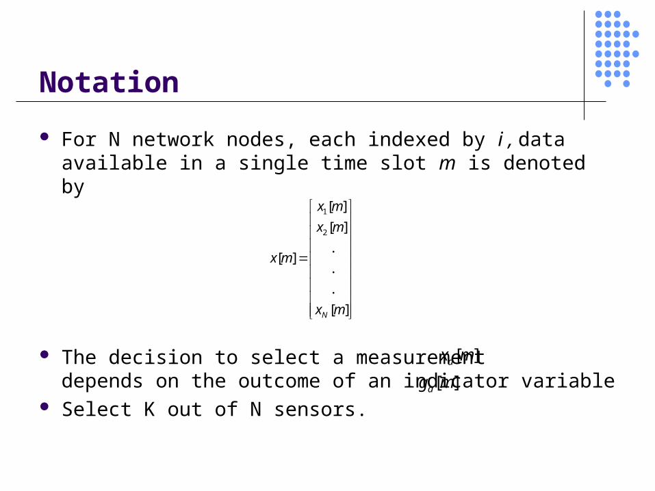
Notation

For N network nodes, each indexed by i , data available in a single time slot m is denoted by

The decision to select a measurement depends on the outcome of an indicator variable

Select K out of N sensors.

1

2

[ ]

[ ]

.[ ]

.

.

[ ]N

x m

x m

x m

x m

[ ]ax m

[ ]ag m

Notation

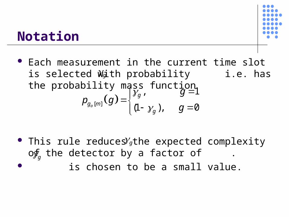
Each measurement in the current time slot is selected with probability i.e. has the probability mass function

This rule reduces the expected complexity of the detector by a factor of .

is chosen to be a small value.

[ ]

, 1

(1 ), 0a

g

g mg

gp g

g

g

g

g

Notation

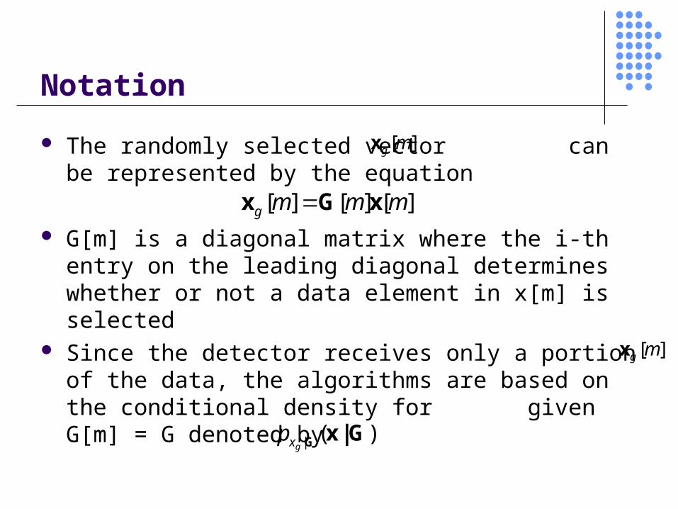
The randomly selected vector can be represented by the equation

G[m] is a diagonal matrix where the i-th entry on the leading diagonal determines whether or not a data element in x[m] is selected

Since the detector receives only a portion of the data, the algorithms are based on the conditional density for given G[m] = G denoted by

[ ] [ ] [ ]g m m mx G x

| ( )gx

p G x | G

[ ]g mx

[ ]g mx

Application to Distributed Signal Processing

Random selection with a small value of can lead to acceptable detector performance

Energy dissipated by communication may also be limited Avoids computational and communicational overhead

that may be incurred from more complicated iteration procedures or centralized coordination

Compatible with ad-hoc networking, clustered or unclustered networks

g

Randomized Selection in Detection

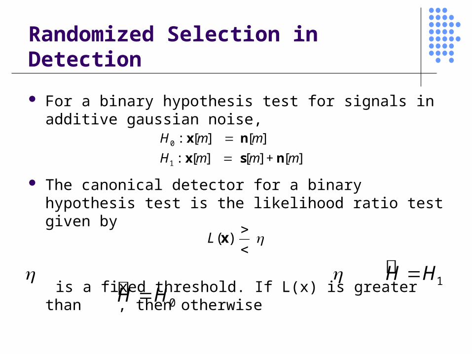
For a binary hypothesis test for signals in additive gaussian noise,

The canonical detector for a binary hypothesis test is the likelihood ratio test given by

is a fixed threshold. If L(x) is greater than , then otherwise

0

1

: [ ] [ ]

: [ ] [ ] + [ ]

H m m

H m m m

x n

x s n

( ) L

x

1H H

0H H

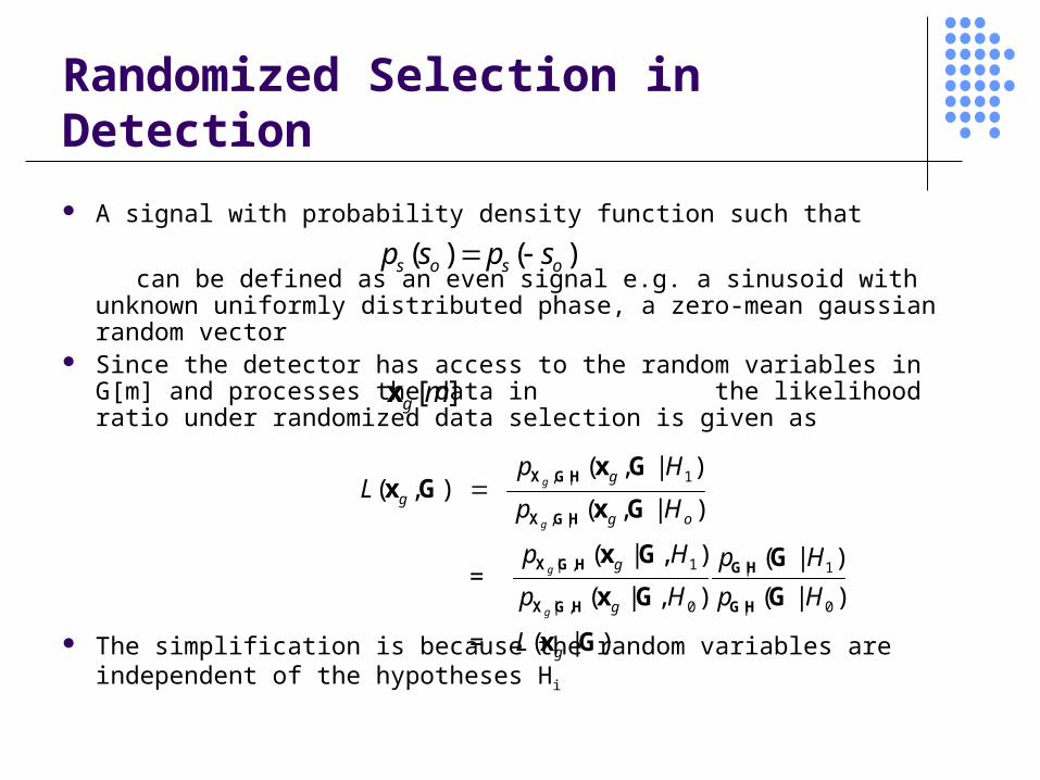
Randomized Selection in Detection

A signal with probability density function such that

can be defined as an even signal e.g. a sinusoid with unknown uniformly distributed phase, a zero-mean gaussian random vector

Since the detector has access to the random variables in G[m] and processes the data in the likelihood ratio under randomized data selection is given as

The simplification is because the random variables are independent of the hypotheses Hi

( ) ( )s o s op s p s

, | 1

, |

| , 1 | 1

| , 0 | 0

( , | )( , )

( , | )

( | , ) ( | ) =

( | , ) ( | )

= ( | )

g

g

g

g

g

gg o

g

g

g

p HL

p H

p H p H

p H p H

L

X G H

X G H

X G H G H

X G H G H

x Gx G

x G

x G G

x G G

x G

[ ]g mx

Randomized Selection in Detection

Likelihood ratio compared to a fixed threshold is optimal under the Neyman-Pearson criterion

Two problems: Determining the threshold can be computationally complex –

requires inversion of:

Requires 2N terms for N samples of data and approximations can be troublesome

G fluctuates although threshold is constant Solution is to fix false alarm rate for each G (Constant False Alarm

Rate detection).

| 0 0( ) ( | ) Pr( ( ) | , )F H gP p H L H GG

G x G

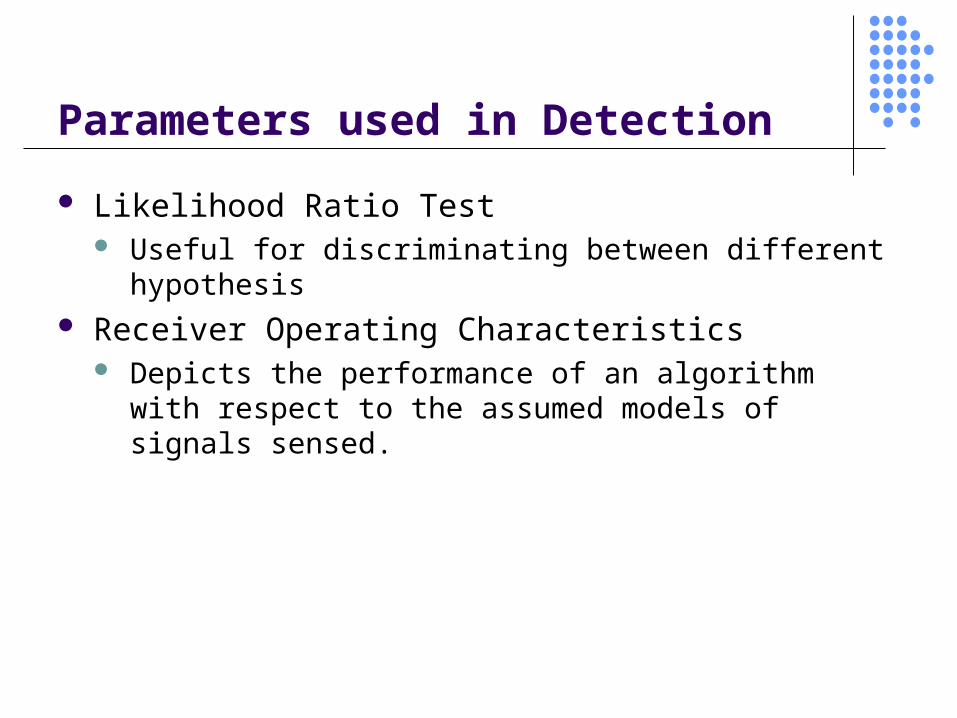
Parameters used in Detection

Likelihood Ratio Test Useful for discriminating between different hypothesis

Receiver Operating Characteristics Depicts the performance of an algorithm with respect to the

assumed models of signals sensed.

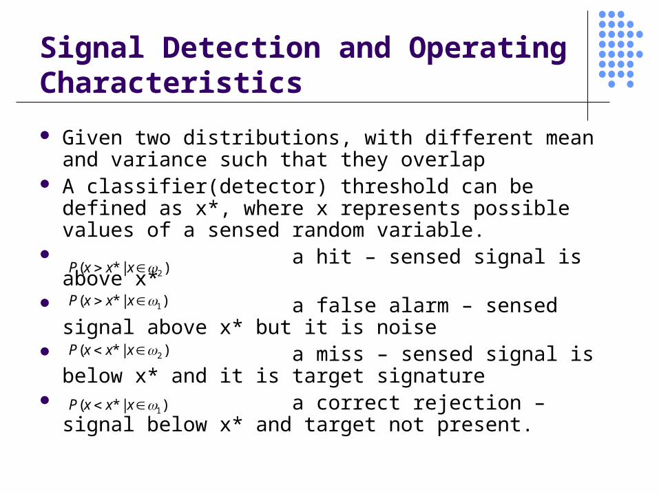
Signal Detection and Operating Characteristics

Given two distributions, with different mean and variance such that they overlap

A classifier(detector) threshold can be defined as x*, where x represents possible values of a sensed random variable.

a hit – sensed signal is above x* a false alarm – sensed signal above x* but it

is noise a miss – sensed signal is below x* and it is

target signature a correct rejection – signal below x* and

target not present.

2( * | )P x x x

1( * | )P x x x

2( * | )P x x x

1( * | )P x x x

Signal Detection and Operating Characteristics

is the discriminability || 10'

d

*x0 1

A hit

False AlarmA miss

Correct rejection

Consider data set vi generated by sampling a sinusoid; under a binary hypothesis test

ni is a Gaussian random variable with zero mean and variance . Given that , probability density is

where u() denotes the unit step function, K is number of selected data

Example – Detecting a Sinusoidal Signal

0

1

: =

: = Acos(2 )

i i

ii i

H x n

vH x n

| 2 21

( | |)( | )

Ki

Ki i

u A cp K

A c

c c

2)2cos(][

i

i

vAmc

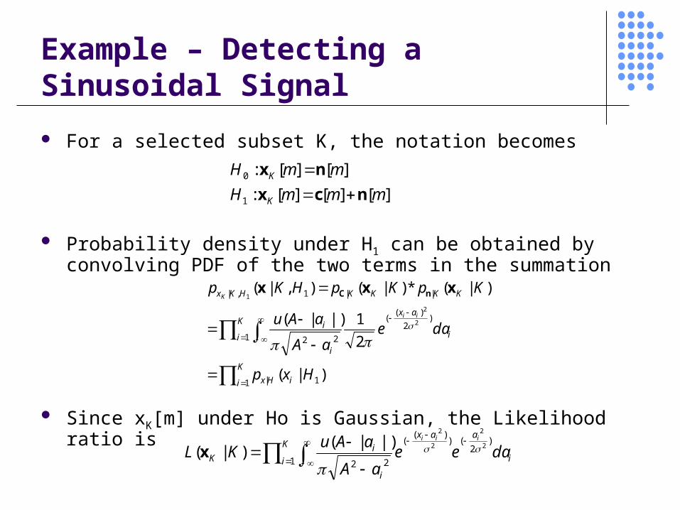
Example – Detecting a Sinusoidal Signal

For a selected subset K, the notation becomes

Probability density under H1 can be obtained by convolving PDF of the two terms in the summation

Since xK[m] under Ho is Gaussian, the Likelihood ratio is

K

i iHx

K

i i

ax

i

i

KKKKHKx

Hxp

daeaA

aAu

KpKpHKp

ii

K

1 1|

1

)2

)((

22

||1,|

)|(

2

1|)|(

)|(*)|(),|(

2

2

1

xxx nC

][][][:

][][:

1

0

mmmH

mmH

K

K

ncx

nx

K

i i

aax

i

iK daee

aA

aAuKL

iii

1

)2

())(

(

22

2

2

2

2

|)|()|(

x

Example – Detecting a Sinusoidal Signal

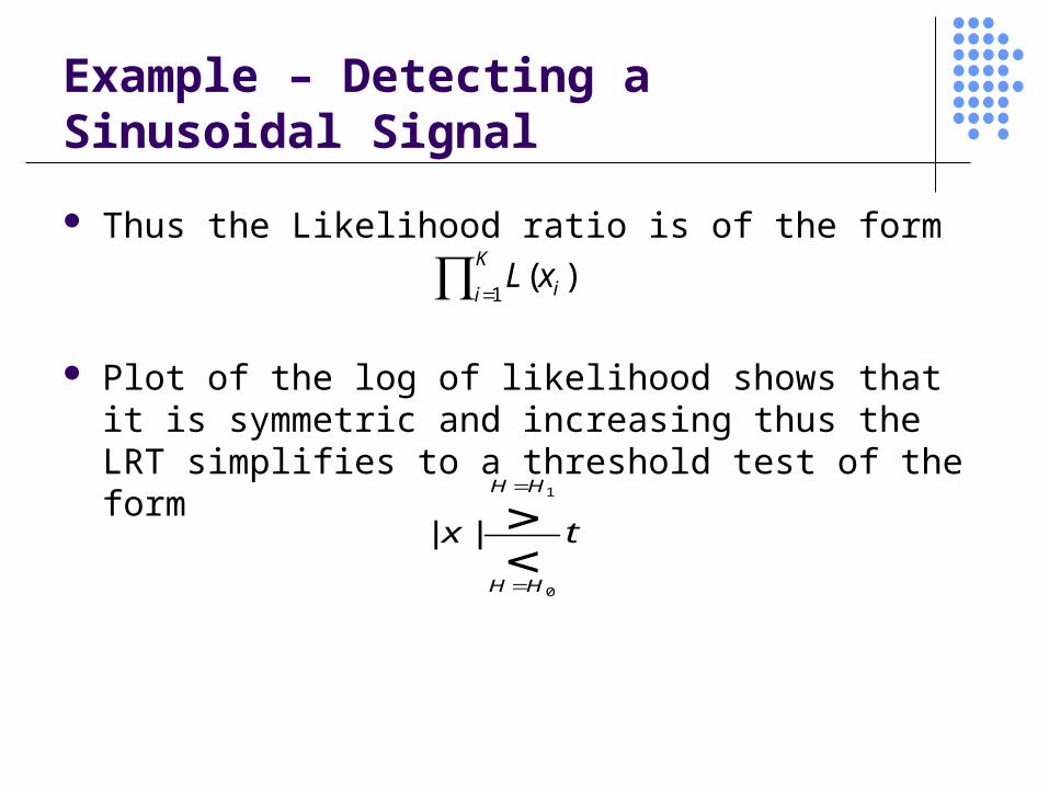
Thus the Likelihood ratio is of the form

Plot of the log of likelihood shows that it is symmetric and increasing thus the LRT simplifies to a threshold test of the form

K

i ixL1).(

tx

HH

HH

0

1

||

Example – Detecting a Sinusoidal Signal

Plot of Log Likelihoods for different A: shows symmetry and monotonicity

Example – Detecting a Sinusoidal Signal - Performance

The ROC can be determined by integrating the conditional densities over the decision region for

ROC calculated from the LRT gives the maximum achievable PD for each false alarm rate

1ˆ HH

t0

),|( 1,| HKpP KHKD Kxx

),|( 0,| HKpP KHKF Kxx

10 FP

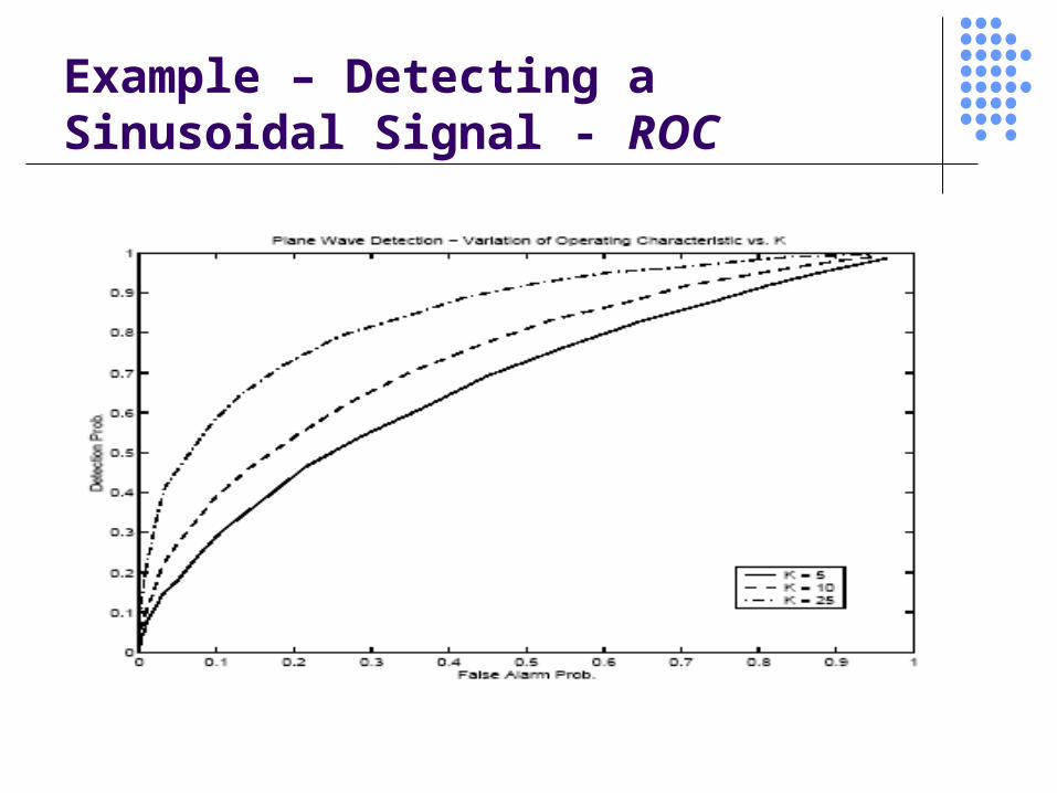
Example – Detecting a Sinusoidal Signal - ROC

Spatial Selection

Variograms Use of Transect

Estimate Variogram along straight line drawn through a region Such an estimate may exhibit directionality except if

underlying process is isotropic

Spatial Selection

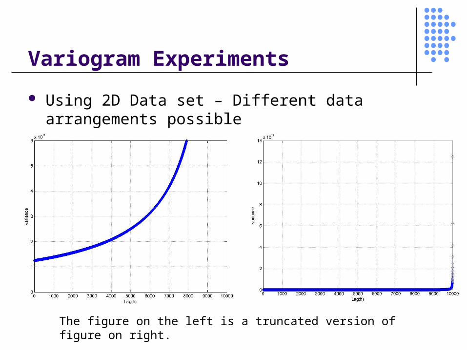
Location of target May allow variable amount of data to be used in estimate

2D May lead different variogram estimates Different data arrangements possible

Spatial Selection

Natural Estimator

where

And is the number of distinct pairs in Robust Estimator

Robust to contamination by outliers [2]

2

( )

12 ( ) ( ( ) ( )) ,

| ( ) |d

i jN

Z ZN

h

h s s hh

( ) ( , ) : ; , 1,...,i j i jN i j n h s s s s h

| ( ) |N h ( )N h

4

1/ 2

( )

1| ( ) ( ) |

| ( ) |2 ( )

(0.457 0.494 / | ( ))

i jN h

Z s Z sN h

hN h

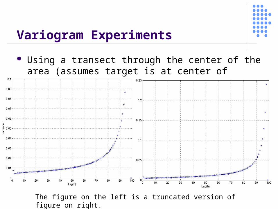
Variogram Experiments

Using a transect through the center of the area (assumes target is at center of sensor area)

The figure on the left is a truncated version of figure on right.

Variogram Experiments

Using 2D Data set – Different data arrangements possible

The figure on the left is a truncated version of figure on right.

Discussions/Comparisons(Randomization)

High dependence on base station/manager node All nodes are active all the time Data may arrive in out-of-order fashion at the base

station Random selection may result in biased selection hence a

one-sided view of phenomenon In multihop routing some of the selected data may be

lost Potential for simple and practical implementation May consume surprising amount of energy (short

network lifetime) Does not collect network state

References

Charles K. Sestok, Maya R. Said, Alan V. Oppenheim, Randomized Data Selection in Detection with applications to distributed Signal Processing, IEEE Proceedings, Nov. 2003.

Cressie Noel A. C., Statistics for Spatial Data, Wiley 1991