Data Mining Tutorial D. A. Dickey CopyrightCopyright © Time and Date AS / Steffen Thorsen...

Data Mining TutorialData Mining Tutorial

D. A. Dickey

April 2012

2013: International Year of Statistics

Data Mining - What is it?• Large datasets• Fast methods• Not significance testing• Topics

– Trees (recursive splitting)– Logistic Regression– Neural Networks– Association Analysis– Nearest Neighbor– Clustering– Etc.

Trees

• A “divisive” method (splits)

• Start with “root node” – all in one group

• Get splitting rules

• Response often binary

• Result is a “tree”

• Example: Loan Defaults

• Example: Framingham Heart Study

• Example: Automobile fatalities

Recursive Splitting

X1=DebtToIncomeRatio

X2 = Age

Pr{default} =0.007 Pr{default} =0.012

Pr{default} =0.0001

Pr{default} =0.003

Pr{default} =0.006

No defaultDefault

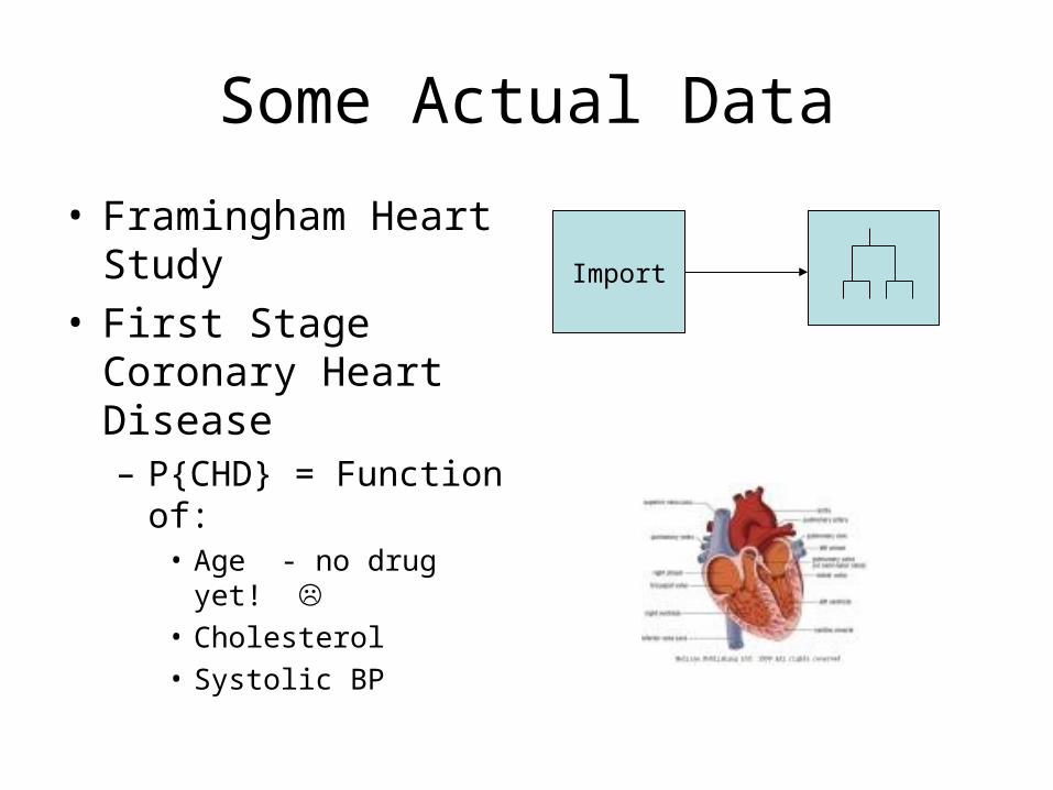
Some Actual Data

• Framingham Heart Study

• First Stage Coronary Heart Disease – P{CHD} = Function of:

• Age - no drug yet! • Cholesterol• Systolic BP

Import

Example of a “tree”

All 1615 patients

Split # 1: Age

“terminal node”Systolic BP

How to make splits?

• Which variable to use?

• Where to split?– Cholesterol > ____– Systolic BP > _____

• Goal: Pure “leaves” or “terminal nodes”

• Ideal split: Everyone with BP>x has problems, nobody with BP<x has problems

Where to Split?

• First review Chi-square tests• Contingency tables

95 5

55 45

Heart DiseaseNo Yes

LowBP

HighBP

100

100

DEPENDENT

75 25

75 25

INDEPENDENT

Heart DiseaseNo Yes

2 Test Statistic • Expect 100(150/200)=75 in upper left if

independent (etc. e.g. 100(50/200)=25)

95

(75)

5

(25)

55

(75)

45

(25)

Heart DiseaseNo Yes

LowBP

HighBP

100

100

150 50 200

allcells ected

ectedobserved

exp

)exp( 22

2(400/75)+2(400/25) = 42.67

Compare to Tables – Significant!WHERE IS HIGH BP CUTOFF???

Measuring “Worth” of a Split

• P-value is probability of Chi-square as great as that observed if independence is true. (Pr {2>42.67} is 6.4E-11)

• P-values all too small.

• Logworth = -log10(p-value) = 10.19

• Best Chi-square max logworth.

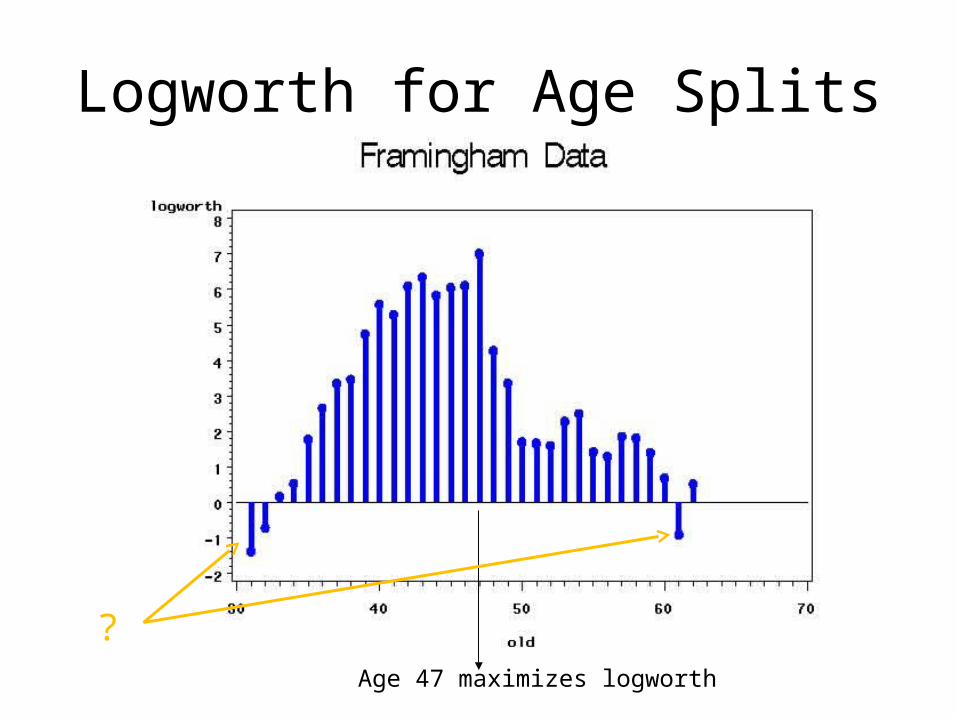
Logworth for Age Splits

Age 47 maximizes logworth

?

How to make splits?

• Which variable to use?

• Where to split?– Cholesterol > ____– Systolic BP > _____

• Idea – We picked BP cutoff to minimize p-value for 2

• What does “significance” mean now?

Multiple testing

• 50 different BPs in data, 49 ways to split • Sunday football highlights always look

good!• If he shoots enough times, even a 95% free

throw shooter will miss.• Tried 49 splits, each has 5% chance of

declaring significance even if there’s no relationship.

Multiple testing

= Pr{ falsely reject hypothesis 1}

= Pr{ falsely reject hypothesis 2}

Pr{ falsely reject one or the other} < 2Desired: 0.05 probabilty or lessSolution: use = 0.05/2Or – compare 2(p-value) to 0.05

Multiple testing

• 50 different BPs in data, m=49 ways to split

• Multiply p-value by 49

• Bonferroni – original idea

• Kass – apply to data mining (trees)

• Stop splitting if minimum p-value is large.

• For m splits, logworth becomes

-log10(m*p-value) ! ! !

Other Split Evaluations

• Gini Diversity Index – { A A A A B A B B C B}– Pick 2, Pr{different} = 1-Pr{AA}-Pr{BB}-Pr{CC}

• 1-[10+6+0]/45=29/45=0.64 LESS DIVERSE

– { A A B C B A A B C C }• 1-[6+3+3]/45 = 33/45 = 0.73 MORE DIVERSE, LESS

PURE

• Shannon Entropy– Larger more diverse (less pure)

– -i pi log2(pi) {0.5, 0.4, 0.1} 1.36 (less diverse){0.4, 0.3, 0.3} 1.74 (more diverse)

Goals

• Split if diversity in parent “node” > summed diversities in child nodes

• Observations should be – Homogeneous (not diverse) within leaves– Different between leaves– Leaves should be diverse

• Framingham tree used Gini for splits

Validation

• Traditional stats – small dataset, need all observations to estimate parameters of interest.

• Data mining – loads of data, can afford “holdout sample”

• Variation: n-fold cross validation– Randomly divide data into n sets– Estimate on n-1, validate on 1– Repeat n times, using each set as holdout.

Pruning

• Grow bushy tree on the “fit data”

• Classify holdout data

• Likely farthest out branches do not improve, possibly hurt fit on holdout data

• Prune non-helpful branches.

• What is “helpful”? What is good discriminator criterion?

Goals• Want diversity in parent “node” > summed

diversities in child nodes

• Goal is to reduce diversity within leaves

• Goal is to maximize differences between leaves

• Use validation average squared error, proportion correct decisions, etc.

• Costs (profits) may enter the picture for splitting or pruning.

Accounting for Costs

• Pardon me (sir, ma’am) can you spare some change?

• Say “sir” to male +$2.00

• Say “ma’am” to female +$5.00

• Say “sir” to female -$1.00 (balm for slapped face)

• Say “ma’am” to male -$10.00 (nose splint)

Including Probabilities

True Gender

M

F

Leaf has Pr(M)=.7, Pr(F)=.3. You say:

Sir Ma’am

0.7 (2)

0.3 (-1)

0.7 (-10)

0.3 (5)

Expected profit is 2(0.7)-1(0.3) = $1.10 if I say “sir” Expected profit is -7+1.5 = -$5.50 (a loss) if I say “Ma’am”Weight leaf profits by leaf size (# obsns.) and sumPrune (and split) to maximize profits.

+$1.10 -$5.50

Additional Ideas

• Forests – Draw samples with replacement (bootstrap) and grow multiple trees.

• Random Forests – Randomly sample the “features” (predictors) and build multiple trees.

• Classify new point in each tree then average the probabilities, or take a plurality vote from the trees

* Cumulative Lift Chart - Go from leaf of most to least predicted response. - Lift is proportion responding in first p% overall population response rate

Lift3.3

1

Regression Trees• Continuous response Y

• Predicted response Pi constant in regions i=1, …, 5

Predict 50

Predict 80

Predict 100

Predict 130 Predict

20

X1

X2

• Predict Pi in cell i.

• Yij jth response in cell i.

• Split to minimize i j (Yij-Pi)2

Predict 50

Predict 80

Predict 100

Predict 130 Predict

20

• Predict Pi in cell i.

• Yij jth response in cell i.

• Split to minimize i j (Yij-Pi)2

Real data example: Traffic accidents in Portugal*Y = injury induced “cost to society”

* Tree developed by Guilhermina Torrao, (used with permission) NCSU Institute for Transportation Research & Education

Help - I ran Into a “tree”

Help - I ran Into a “tree”

Cool < ------------------------ > Nerdy

“Analytics” ------------------- “Statistics”“Predictive Modeling” ------------------ “Regression”

Another major tool:Regression (OLS: ordinary least squares)

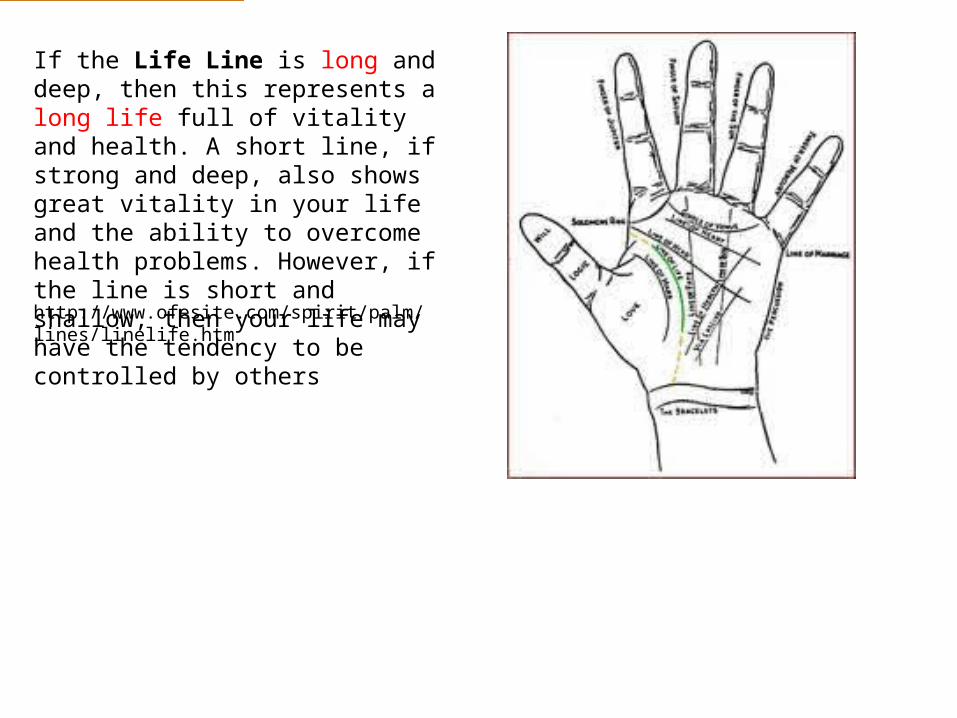
If the Life Line is long and deep, then this represents a long life full of vitality and health. A short line, if strong and deep, also shows great vitality in your life and the ability to overcome health problems. However, if the line is short and shallow, then your life may have the tendency to be controlled by others

http://www.ofesite.com/spirit/palm/lines/linelife.htm

Wilson & Mather JAMA 229 (1974)

X=life line length Y=age at death

Result: Predicted Age at Death = 79.24 – 1.367(lifeline) (Is this “real”??? Is this repeatable???)

proc sgplot; scatter Y=age X=line; reg Y=age X=line; run ;

We Use LEAST SQUARES

Squared residuals sum to 9609

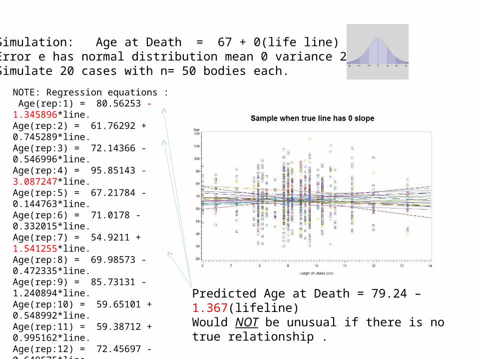
Simulation: Age at Death = 67 + 0(life line) + eError e has normal distribution mean 0 variance 200.Simulate 20 cases with n= 50 bodies each.

NOTE: Regression equations : Age(rep:1) = 80.56253 - 1.345896*line.Age(rep:2) = 61.76292 + 0.745289*line.Age(rep:3) = 72.14366 - 0.546996*line.Age(rep:4) = 95.85143 - 3.087247*line.Age(rep:5) = 67.21784 - 0.144763*line.Age(rep:6) = 71.0178 - 0.332015*line.Age(rep:7) = 54.9211 + 1.541255*line.Age(rep:8) = 69.98573 - 0.472335*line.Age(rep:9) = 85.73131 - 1.240894*line.Age(rep:10) = 59.65101 + 0.548992*line.Age(rep:11) = 59.38712 + 0.995162*line.Age(rep:12) = 72.45697 - 0.649575*line.Age(rep:13) = 78.99126 - 0.866334*line.Age(rep:14) = 45.88373 + 2.283475*line.Age(rep:15) = 59.28049 + 0.790884*line.Age(rep:16) = 73.6395 - 0.814287*line.Age(rep:17) = 70.57868 - 0.799404*line.Age(rep:18) = 72.91134 - 0.821219*line.Age(rep:19) = 55.46755 + 1.238873*line.Age(rep:20) = 63.82712 + 0.776548*line.

Predicted Age at Death = 79.24 – 1.367(lifeline)Would NOT be unusual if there is no true relationship .

Conclusion: Estimated slopes varyStandard deviation (estimated) of sample slopes = “Standard error”Compute t = (estimate – hypothesized)/standard errorp-value is probability of larger |t| when hypothesis is correct (e.g. 0 slope)p-value is sum of two tail areas.Traditionally p<0.05 implies hypothesized value is wrong. p>0.05 is inconclusive.

Distribution of tUnder H0

proc reg data=life; model age=line; run;

Parameter Estimates

Parameter StandardVariable DF Estimate Error t Value Pr > |t|Intercept 1 79.23341 14.83229 5.34 <.0001Line 1 -1.36697 1.59782 -0.86 0.3965

Area 0.19825Area 0.19825 0.39650

-0.86 0.86

Conclusion: insufficient evidence against the hypothesis of no linear relationship.

H0:H1:

H0: InnocenceH1: Guilt

Beyond reasonable doubt

P<0.05

H0: True slope is 0 (no association)H1: True slope is not 0 P=0.3965

Simulation: Age at Death = 67 + 0(life line) + eError e has normal distribution mean 0 variance 200. WHY?Simulate 20 cases with n= 50 bodies each.

Want estimate of variability around the true line. True variance is Use sums of squared residuals (SS).

Sum of squared residuals from the mean is “SS(total)” 9755Sum of squared residuals around the line is “SS(error)” 9609

(1) SS(total)-SS(error) is SS(model) = 146(2) Variance estimate is SS(error)/(degrees of freedom) = 200(3) SS(model)/SS(total) is R2, i.e. proportion of variablity “explained” by the model.

2

Analysis of Variance

Sum of MeanSource DF Squares Square F Value Pr > FModel 1 146.51753 146.51753 0.73 0.3965Error 48 9608.70247 200.18130Corrected Total 49 9755.22000

Root MSE 14.14854 R-Square 0.0150

Those Mysterious “Degrees of Freedom” (DF)

First Martian information about average height 0 information about variation.

2nd Martian gives first piece of information (DF) about error variance around mean.

n Martiansn-1 DF for error (variation)

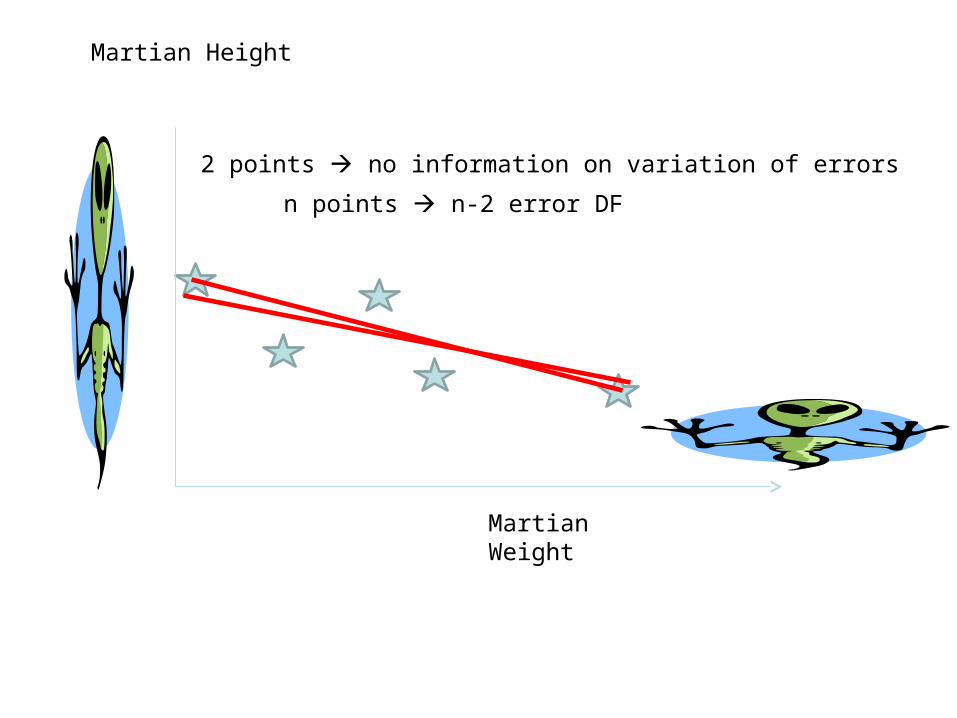
Martian Height

Martian Weight

2 points no information on variation of errors

n points n-2 error DF

How Many Table Legs? (regress Y on X1, X2)

X1

X2error

Fit a plane n-3 (37) error DF (2 “model” DF, n-1=39 “total” DF)

Regress Y on X1 X2 … X7 n-8 error DF (7 “model” DF, n-1 “total” DF)

Sum of MeanSource DF Squares SquareModel 2 32660996 16330498Error 37 1683844 45509Corrected Total 39 34344840

Three legs will all touch the floor.

Fourth leg gives first chance to measure error (first error DF).

Extension: Multiple Regression

Issues: (1) Testing joint importance versus individual significance

(2) Prediction versus modeling individual effects

(3) Collinearity (correlation among inputs)

Example: Hypothetical company’s sales Y depend on TV advertising X1 and Radio Advertising X2.

Y = 0 + 1X1 + 2X2 +e

Jointly critical (can’t omit both!!)

Two engine plane can still fly if engine #1 failsTwo engine plane can still fly if engine #2 failsNeither is critical individually

Data Sales; length sval $8; length cval $8; input store TV radio sales; (more code)cards; 1 869 868 9089 2 836 820 8290 (more data) 40 969 961 10130

proc g3d data=sales; scatter radio*TV=sales/shape=sval color=cval zmin=8000;run;

TV

Sales

Radio

Conclusion: Can predict well with just TV, just radio, or both!

SAS code: proc reg data=next; model sales = TV radio;


Sum of MeanSource DF Squares Square F Value Pr > FModel 2 32660996 16330498 358.84 <.0001 (Can’t omit both)Error 37 1683844 45509Corrected Total 39 34344840

Root MSE 213.32908 R-Square 0.9510 Explaining 95% of variation in sales

Parameter Estimates

Parameter StandardVariable DF Estimate Error t Value Pr > |t|Intercept 1 531.11390 359.90429 1.48 0.1485TV 1 5.00435 5.01845 1.00 0.3251 (can omit TV)radio 1 4.66752 4.94312 0.94 0.3512 (can omit radio)

Estimated Sales = 531 + 5.0 TV + 4.7 radio with error variance 45509 (standard deviation 213).

TV approximately equal to radio so, approximately

Estimated Sales = 531 + 9.7 TV or

Estimated Sales = 531 + 9.7 radio

Summary:

Good predictions given by Sales = 531 + 5.0 x TV + 4.7 x Radio or Sales = 479 + 9.7 x TV orSales = 612 + 9.6 x Radio or

(lots of others)

Why the confusion?The evil Multicollinearity!!

(correlated X’s)

Multicollinearity can be diagnosed by looking at principal components (axes of variation)

Variance along PC axes “eigenvalues” of correlation matrixDirection axes point “eigenvectors” of correlation matrix

TV $

Radio $

Principal Component Axis 1

Principal Component Axis 2

Proc Corr; Var TV radio sales;

Pearson Correlation Coefficients, N = 40 Prob > |r| under H0: Rho=0

TV radio sales

TV 1.00000 0.99737 0.97457 <.0001 <.0001

radio 0.99737 1.00000 0.97450 <.0001 <.0001

sales 0.97457 0.97450 1.00000 <.0001 <.0001

Grades vs. IQ and Study Time

Data tests; input IQ Study_Time Grade; IQ_S = IQ*Study_Time; cards; 105 10 75110 12 79120 6 68116 13 85122 16 91130 8 79114 20 98102 15 76 ; Proc reg data=tests; model Grade = IQ; Proc reg data=tests; model Grade = IQ Study_Time;

Parameter StandardVariable DF Estimate Error t Value Pr > |t|Intercept 1 62.57113 48.24164 1.30 0.2423IQ 1 0.16369 0.41877 0.39 0.7094

Parameter StandardVariable DF Estimate Error t Value Pr > |t|Intercept 1 0.73655 16.26280 0.05 0.9656IQ 1 0.47308 0.12998 3.64 0.0149Study_Time 1 2.10344 0.26418 7.96 0.0005

Contrast: TV advertising looses significance when radio is added. IQ gains significance when study time is added.

Model for Grades: Predicted Grade = 0.74 + 0.47 x IQ + 2.10 x Study Time

Question: Does an extra hour of study really deliver 2.10 points for everyone regardless of IQ? Current model only allows this.

“Interaction” model: Predicted Grade = 72.21 0.13 x IQ 4.11 x Study Time + 0.053 x IQ x Study Time = (72.21 0.13 x IQ )+( 4.11 + 0.053 x IQ )x Study Time

IQ = 102 predicts Grade = (72.21-13.26)+(5.41-4.11) x Study Time = 58.95+ 1.30 x Study Time IQ = 122 predicts Grade = (72.21-15.86)+(6.47-4.11) x Study Time = 56.35 + 2.36 x Study Time

proc reg; model Grade = IQ Study_Time IQ_S;

Sum of Mean Source DF Squares Square F Value Pr > F

Model 3 610.81033 203.60344 26.22 0.0043 Error 4 31.06467 7.76617 Corrected Total 7 641.87500

Root MSE 2.78678 R-Square 0.9516 Parameter Standard Variable DF Estimate Error t Value Pr > |t|

Intercept 1 72.20608 54.07278 1.34 0.2527 IQ 1 -0.13117 0.45530 -0.29 0.7876 Study_Time 1 -4.11107 4.52430 -0.91 0.4149 IQ_S 1 0.05307 0.03858 1.38 0.2410

(1) Adding interaction makes everything insignificant (individually) !(2) Do we need to omit insignificant terms until only significant ones remain?(3) Has an acquitted defendant proved his innocence?(4) Common sense trumps statistics!

Slope = 1.30

Slope = 2.36

Logistic Regression • “Trees” seem to be main tool.

• Logistic – another classifier

• Older – “tried & true” method

• Predict probability of response from input variables (“Features”)

• Linear regression gives infinite range of predictions

• 0 < probability < 1 so not linear regression.

Example: Seat Fabric Ignition

• Flame exposure time = X

• Ignited Y=1, did not ignite Y=0– Y=0, X= 3, 5, 9 10 , 13, 16 – Y=1, X = 7, 11, 12, 14, 15, 17, 25, 30

• Q=(1-p1)(1-p2)p3(1-p4)(1-p5)p6p7(1-p8)p9p10(1-p11)p12p13p14

• p’s all different : pi=exp(a+bXi) /(1+exp(a+bXi))

• Find a,b to maximize Q(a,b)

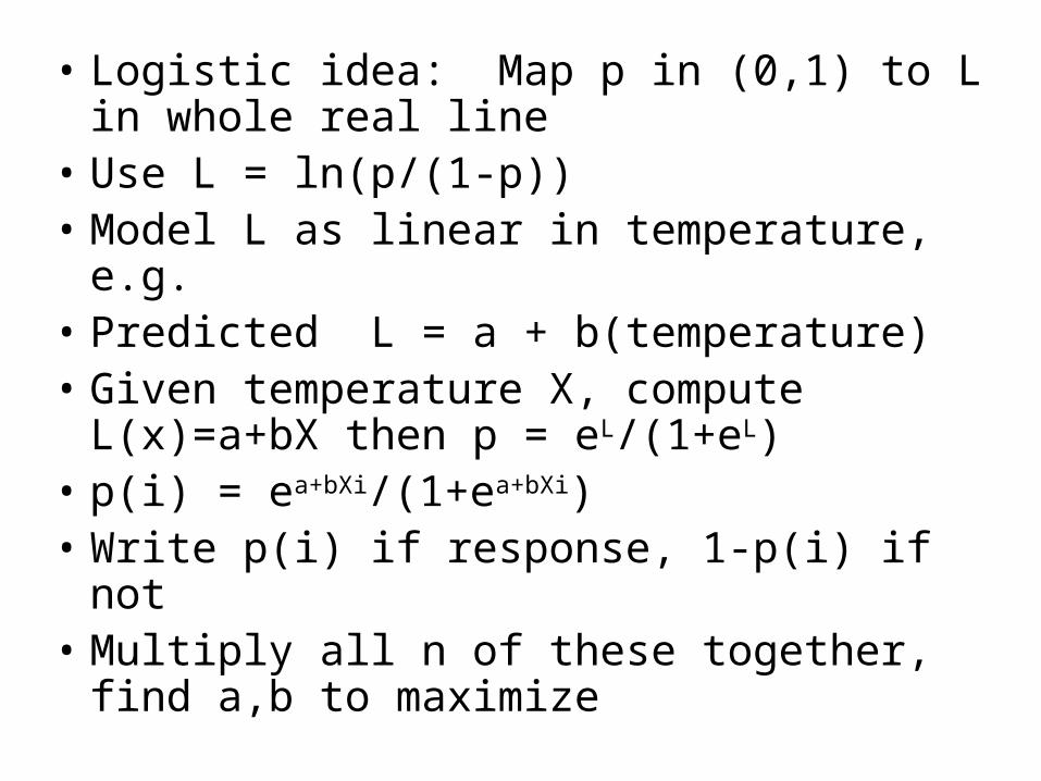
• Logistic idea: Map p in (0,1) to L in whole real line

• Use L = ln(p/(1-p))• Model L as linear in temperature, e.g.• Predicted L = a + b(temperature)• Given temperature X, compute L(x)=a+bX

then p = eL/(1+eL)• p(i) = ea+bXi/(1+ea+bXi) • Write p(i) if response, 1-p(i) if not• Multiply all n of these together, find a,b to

maximize

DATA LIKELIHOOD; ARRAY Y(14) Y1-Y14; ARRAY X(14) X1-X14; DO I=1 TO 14; INPUT X(I) y(I) @@; END; DO A = -3 TO -2 BY .025; DO B = 0.2 TO 0.3 BY .0025; Q=1; DO i=1 TO 14; L=A+B*X(i); P=EXP(L)/(1+EXP(L)); IF Y(i)=1 THEN Q=Q*P; ELSE Q=Q*(1-P); END; IF Q<0.0006 THEN Q=0.0006; OUTPUT; END;END; CARDS; 3 0 5 0 7 1 9 0 10 0 11 1 12 1 13 0 14 1 15 1 16 0 17 1 25 1 30 1 ;

Generate Q for array of (a,b) values

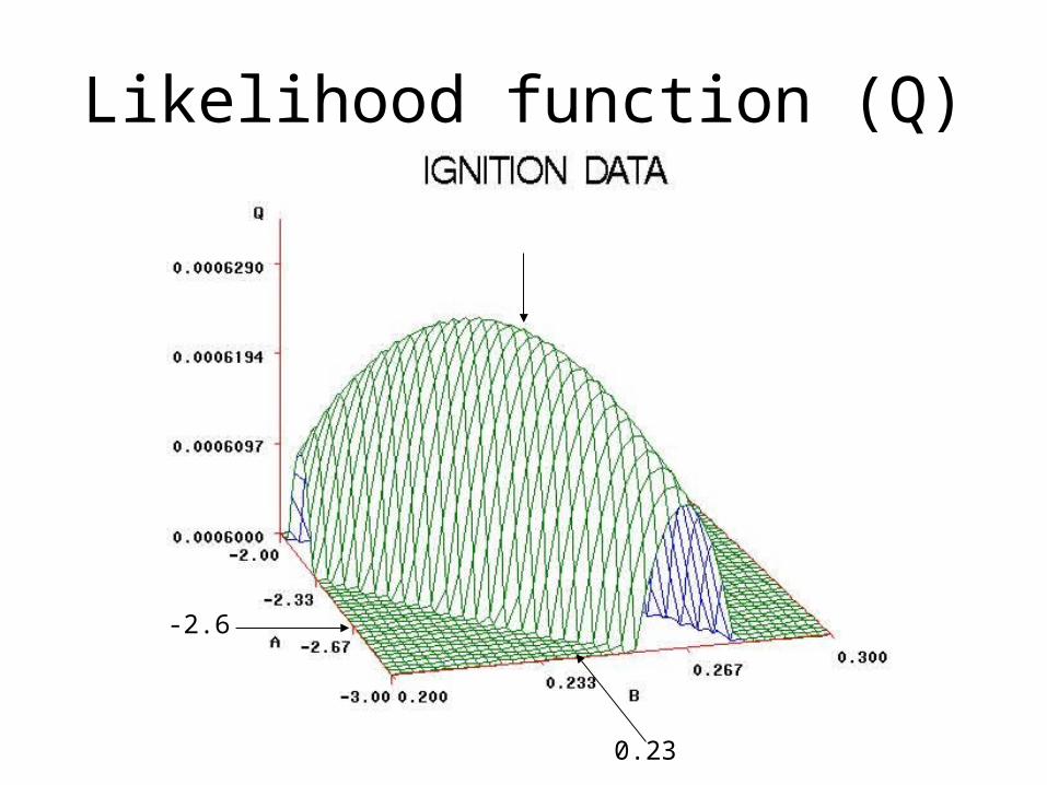
Likelihood function (Q)

-2.6

0.23

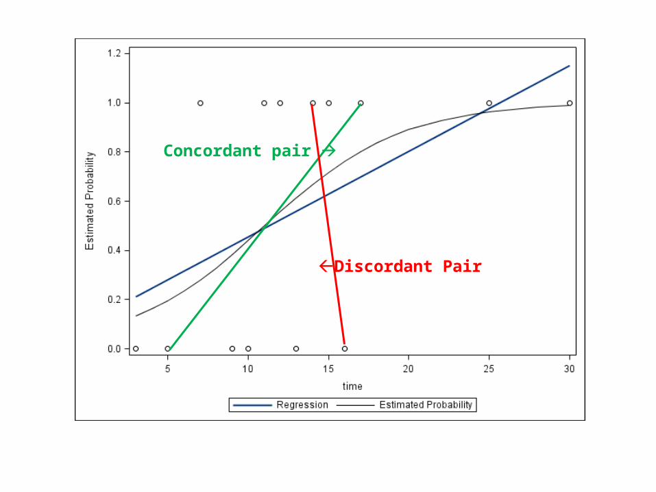
Concordant pair

Discordant Pair

IGNITION DATA The LOGISTIC Procedure Analysis of Maximum Likelihood Estimates Standard WaldParameter DF Estimate Error Chi-Square Pr > ChiSqIntercept 1 -2.5879 1.8469 1.9633 0.1612TIME 1 0.2346 0.1502 2.4388 0.1184

Association of Predicted Probabilities and Observed Responses

Percent Concordant 79.2 Somers' D 0.583Percent Discordant 20.8 Gamma 0.583Percent Tied 0.0 Tau-a 0.308Pairs 48 c 0.792

Example: Shuttle Missions

• O-rings failed in Challenger disaster• Low temperature• Prior flights “erosion” and “blowby” in O-rings• Feature: Temperature at liftoff• Target: problem (1) - erosion or blowby vs. no

problem (0)

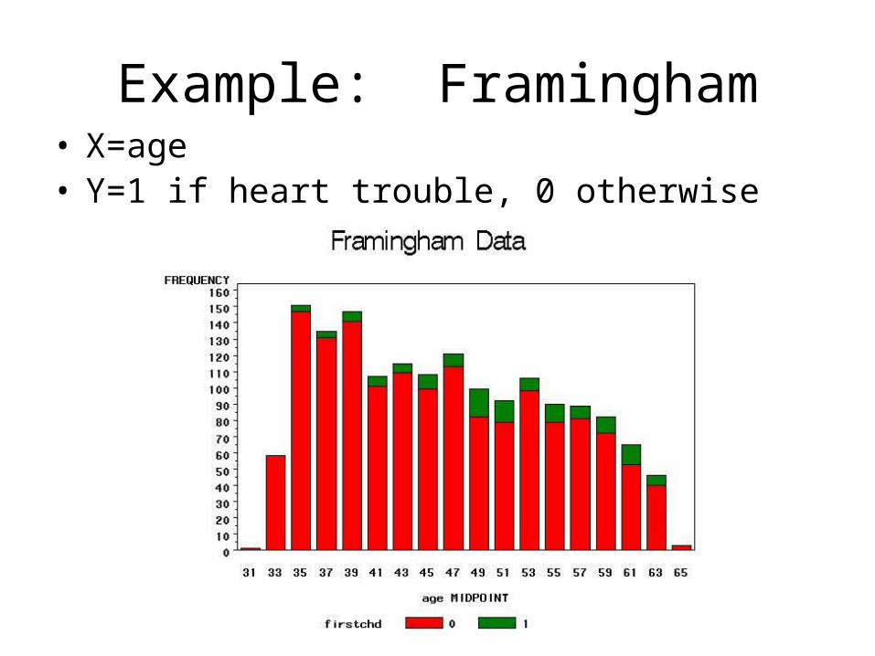
Example: Framingham• X=age • Y=1 if heart trouble, 0 otherwise

Framingham

The LOGISTIC Procedure

Analysis of Maximum Likelihood Estimates

Standard WaldParameter DF Estimate Error Chi-Square Pr>ChiSq

Intercept 1 -5.4639 0.5563 96.4711 <.0001age 1 0.0630 0.0110 32.6152 <.0001

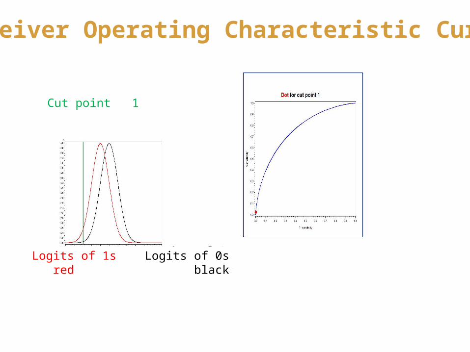
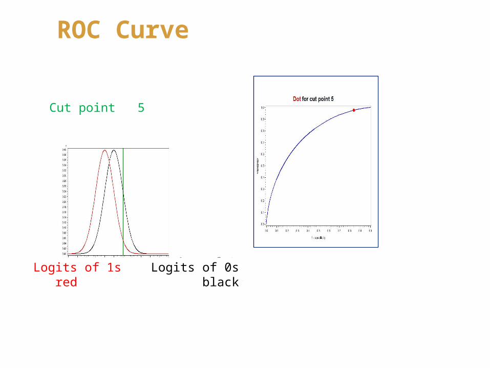
Receiver Operating Characteristic Curve

Logits of 1s Logits of 0s red black

Cut point 1


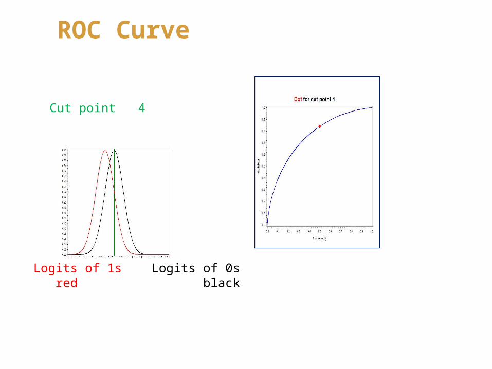
ROC Curve


Cut point 2


ROC Curve


Cut point 3


ROC Curve

Cut point 3.5


ROC Curve

Cut point 4


ROC Curve


Cut point 5


ROC Curve

Cut point 6


Unsupervised Learning• We have the “features” (predictors)

• We do NOT have the response even on a training data set (UNsupervised)

• Clustering– Agglomerative

• Start with each point separated

– Divisive • Start with all points in one cluster then spilt

– Direct• State # clusters beforehand

EM CLUSTER NODE

• Step 1 – find (k=50) “seeds” as separated as possible

• Step 2 – cluster points to nearest seed (iterate – “k-means clustering”)

• Step 3 – aggregate clusters using Ward’s method & determine appropriate number of clusters – new k

• Step 4 – Use k means with this new k.

Clusters as Created

As Clustered – PROC FASTCLUS

Cubic Clustering Criterion (to decide # of Clusters)

• Divide random scatter of (X,Y) points into 4 quadrants

• Pooled within cluster variation much less than overall variation

• Large variance reduction• Big R-square despite no real clusters• CCC compares random scatter R-square

to what you got to decide #clusters• 3 clusters for “macaroni” data.

Classification Variables (dummy variables, indicator variables)

Predicted Accidents = 1181 + 2579 X11 X11 is 1 in November, 0 elsewhere. Interpretation: In November, predict 1181+2579(1) = 3660. In any other month predict 1181 + 2579(0) = 1181. 1181 is average of other months. 2579 is added November effect (vs. average of others)

Model for NC Crashes involving Deer: Proc reg data=deer; model deer = X11;


Sum of MeanSource DF Squares Square F Value Pr > FModel 1 30473250 30473250 90.45 <.0001Error 58 19539666 336891Corrected Total 59 50012916


Parameter StandardVariable Label DF Estimate Error t Value Pr > |t|Intercept Intercept 1 1181.09091 78.26421 15.09 <.0001X11 1 2578.50909 271.11519 9.51 <.0001

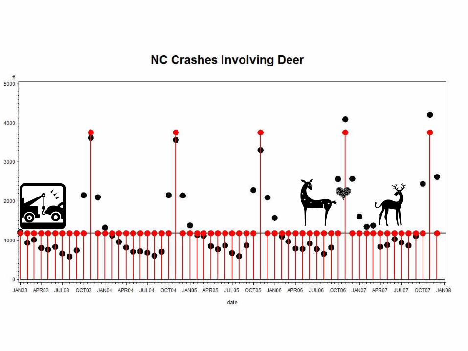
Looks like December and October need dummies too!Proc reg data=deer; model deer = X10 X11 X12;


Sum of MeanSource DF Squares Square F Value Pr > F

Model 3 46152434 15384145 223.16 <.0001Error 56 3860482 68937Corrected Total 59 50012916


Parameter StandardVariable DF Estimate Error t Value Pr > |t|Intercept 1 929.40000 39.13997 23.75 <.0001X10 1 1391.20000 123.77145 11.24 <.0001X11 1 2830.20000 123.77145 22.87 <.0001X12 1 1377.40000 123.77145 11.13 <.0001

Average of Jan through Sept. is 929 crashes per month. Add 1391 in October, 2830 in November, 1377 in December.

date x10 x11 x12

JAN03 0 0 0FEB03 0 0 0MAR03 0 0 0APR03 0 0 0MAY03 0 0 0JUN03 0 0 0JUL03 0 0 0AUG03 0 0 0SEP03 0 0 0OCT03 1 0 0NOV03 0 1 0DEC03 0 0 1JAN04 0 0 0FEB04 0 0 0MAR04 0 0 0APR04 0 0 0MAY04 0 0 0JUN04 0 0 0JUL04 0 0 0AUG04 0 0 0SEP04 0 0 0OCT04 1 0 0NOV04 0 1 0DEC04 0 0 1

What the heck – let’s do all but one (need “average of rest” so must leave out at least one)Proc reg data=deer; model deer = X1 X2 … X10 X11; Analysis of Variance



Parameter Estimates

Parameter StandardVariable Label DF Estimate Error t Value Pr > |t|

Intercept Intercept 1 2306.80000 81.42548 28.33 <.0001X1 1 -885.80000 115.15301 -7.69 <.0001X2 1 -1181.40000 115.15301 -10.26 <.0001X3 1 -1220.20000 115.15301 -10.60 <.0001X4 1 -1486.80000 115.15301 -12.91 <.0001X5 1 -1526.80000 115.15301 -13.26 <.0001X6 1 -1433.00000 115.15301 -12.44 <.0001X7 1 -1559.20000 115.15301 -13.54 <.0001X8 1 -1646.20000 115.15301 -14.30 <.0001X9 1 -1457.20000 115.15301 -12.65 <.0001X10 1 13.80000 115.15301 0.12 0.9051X11 1 1452.80000 115.15301 12.62 <.0001

Average of rest is just December mean 2307. Subtract 886 in January, add 1452 in November. October (X10) is not significantly different than December.

negative

positive

Add date (days since Jan 1 1960 in SAS) to capture trendProc reg data=deer; model deer = date X1 X2 … X10 X11; Analysis of Variance



Parameter Estimates

Parameter StandardVariable Label DF Estimate Error t Value Pr > |t|Intercept Intercept 1 -1439.94000 547.36656 -2.63 0.0115X1 1 -811.13686 82.83115 -9.79 <.0001X2 1 -1113.66253 82.70543 -13.47 <.0001X3 1 -1158.76265 82.60154 -14.03 <.0001X4 1 -1432.28832 82.49890 -17.36 <.0001X5 1 -1478.99057 82.41114 -17.95 <.0001X6 1 -1392.11624 82.33246 -16.91 <.0001X7 1 -1525.01849 82.26796 -18.54 <.0001X8 1 -1618.94416 82.21337 -19.69 <.0001X9 1 -1436.86982 82.17106 -17.49 <.0001X10 1 27.42792 82.14183 0.33 0.7399X11 1 1459.50226 82.12374 17.77 <.0001date 1 0.22341 0.03245 6.88 <.0001

Trend is 0.22 more accidents per day (1 per 5 days) and is significantly different from 0.

Neural Networks

• Very flexible functions• “Hidden Layers” • “Multilayer Perceptron”

Logistic function of

Logistic functions

Of data

outputinputs

Arrows represent linear combinations of “basis functions,” e.g. logistic curves (hyperbolic tangents)

b1

Y

p1

Example: Y = a + b1 p1 + b2 p2 + b3 p3 Y = 4 + p1+ 2 p2 - 4 p3

b2p2

p3

b3

• Should always use holdout sample

• Perturb coefficients to optimize fit (fit data)– Nonlinear search algorithms

• Eliminate unnecessary complexity using holdout data.

• Other basis sets– Radial Basis Functions– Just normal densities (bell shaped) with

adjustable means and variances.

Statistics to Data Mining Dictionary

Statistics Data Mining (nerdy) (cool)

Independent variables FeaturesDependent variable TargetEstimation Training, Supervised LearningClustering Unsupervised Learning

Prediction ScoringSlopes, Betas Weights (Neural nets)Intercept Bias (Neural nets)

Composition of Hyperbolic Neural NetworkTangent FunctionsRadial Basis Function Normal Density and my personal favorite…Type I and Type II Errors Confusion Matrix

Association Analysis

• Market basket analysis – What they’re doing when they scan your “VIP”

card at the grocery– People who buy diapers tend to also buy

_________ (beer?)– Just a matter of accounting but with new

terminology (of course ) – Examples from SAS Appl. DM Techniques, by

Sue Walsh:

Termnilogy

• Baskets: ABC ACD BCD ADE BCE

• Rule Support Confidence

• X=>Y Pr{X and Y} Pr{Y|X}

• A=>D 2/5 2/3

• C=>A 2/5 2/4

• B&C=>D 1/5 1/3 ABC ACD BCD ADE BCE

Don’t be Fooled!• Lift = Confidence /Expected Confidence if Independent

Checking

Saving

No

(1500)

Yes

(8500) (10000)

No 500 3500 4000

Yes 1000 5000 6000

SVG=>CHKG Expect 8500/10000 = 85% if independentObserved Confidence is 5000/6000 = 83%Lift = 83/85 < 1. Savings account holders actually LESS likely than others to have checking account !!!

TEXT MINING

Hypothetical collection of e-mails (“corpus”) from analytics students:

John, message 1: There’s a good cook there.Susan, message 1: I have an analytics practicum then.Susan, message 2: I’ll be late from analytics. John, message 2: Shall we take the kids to a movie?John, message 3: Later we can eat what I cooked yesterday. (etc.) Compute word counts: analytics cook_n cook_v kids late movie practicum John 0 1 1 1 1 1 0Susan 2 0 0 0 1 0 1

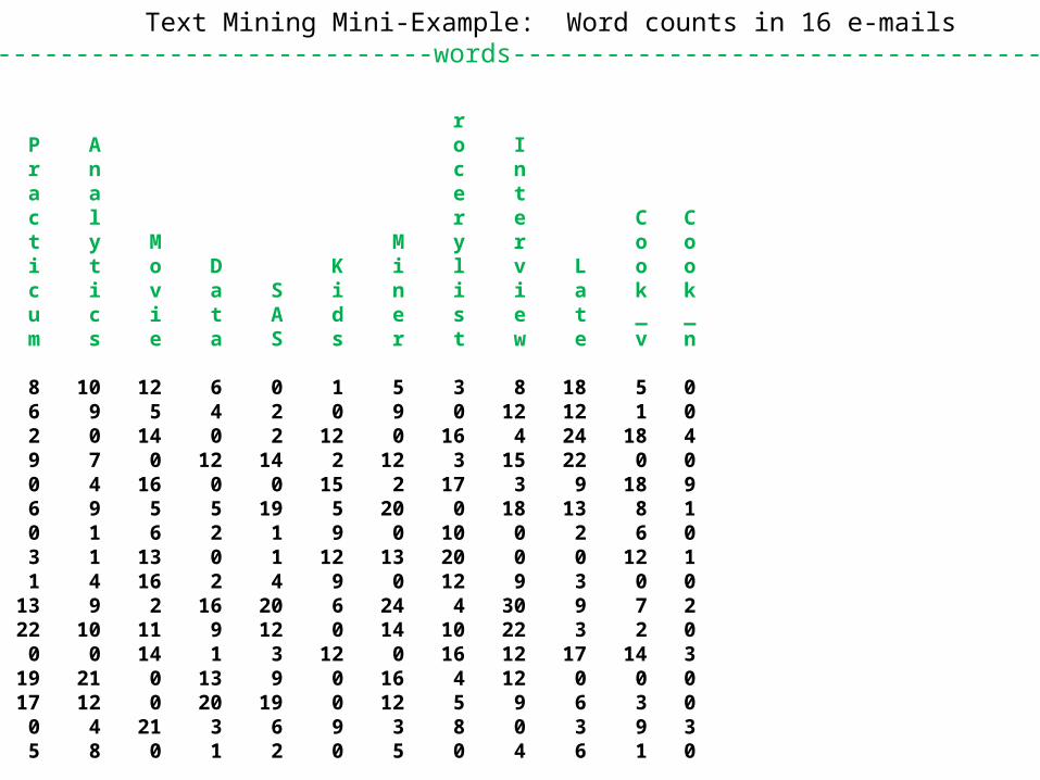
Text Mining Mini-Example: Word counts in 16 e-mails--------------------------------words-----------------------------------------

G r P A o I r n c n s a a e t t c l r e C C u t y M M y r o o d i t o D K i l v L o o e J c i v a S i n i i a k k n o u c i t A d e s e t _ _ t b m s e a S s r t w e v n

1 5 8 10 12 6 0 1 5 3 8 18 5 0 2 5 6 9 5 4 2 0 9 0 12 12 1 0 3 0 2 0 14 0 2 12 0 16 4 24 18 4 4 8 9 7 0 12 14 2 12 3 15 22 0 0 5 0 0 4 16 0 0 15 2 17 3 9 18 9 6 10 6 9 5 5 19 5 20 0 18 13 8 1 7 1 0 1 6 2 1 9 0 10 0 2 6 0 8 2 3 1 13 0 1 12 13 20 0 0 12 1 9 4 1 4 16 2 4 9 0 12 9 3 0 0 10 26 13 9 2 16 20 6 24 4 30 9 7 2 11 19 22 10 11 9 12 0 14 10 22 3 2 0 12 2 0 0 14 1 3 12 0 16 12 17 14 3 13 16 19 21 0 13 9 0 16 4 12 0 0 0 14 14 17 12 0 20 19 0 12 5 9 6 3 0 15 1 0 4 21 3 6 9 3 8 0 3 9 3 16 3 5 8 0 1 2 0 5 0 4 6 1 0

Eigenvalues of the Correlation Matrix Eigenvalue Difference Proportion Cumulative

1 7.49896782 5.55500483 0.5768 0.5768 2 1.94396299 0.72530783 0.1495 0.7264 3 1.21865516 0.60395731 0.0937 0.8201 4 0.61469785 0.10154782 0.0473 0.8674 5 0.51315004 0.09053762 0.0395 0.9069 6 0.42261242 0.10571506 0.0325 0.9394 7 0.31689737 0.09680618 0.0244 0.9638 8 0.22009119 0.11988842 0.0169 0.9807 9 0.10020277 0.02215831 0.0077 0.988410 0.07804446 0.01933787 0.0060 0.994411 0.05870659 0.04670677 0.0045 0.998912 0.01199982 0.00998828 0.0009 0.999813 0.00201154 0.0002 1.0000

58% of the variation in these 12-dimensional vectors occurs in oneDimension (P1)

Prin1

Job 0.317700 Practicum 0.318654 Analytics 0.306205 Movie -.283351 Data 0.314980 SAS 0.279258 Kids -.309731 Miner 0.290127 Grocerylist -.269651 Interview 0.261794 Late -.049560 Cook_v -.267515 Cook_n -.225621

P1

P2

Plotting 2 words only(analytics, family)

Prin1

Job 0.317700 Practicum 0.318654 Analytics 0.306205 Movie -.283351 Data 0.314980 SAS 0.279258 Kids -.309731 Miner 0.290127 Grocerylist -.269651 Interview 0.261794 Late -.049560 Cook_v -.267515 Cook_n -.225621

weights

My counts

.

.3000100001000

My scoreOn P1

3(.3177)+.31498+.26179_______1.530

My score 1.53

PROC CLUSTER (single linkage) on P1 scores of 16 documents (students)

G r P A o I d r n c n o C a a e t c L c l r e C C u U P t y M M y r o o m S r i t o D K i l v L o o e T i J c i v a S i n i i a k k n E n o u c i t A d e s e t _ _ t R 1 b m s e a S s r t w e v n

5 2 -4.18243 0 0 4 16 0 0 15 2 17 3 9 18 9 3 2 -3.62271 0 2 0 14 0 2 12 0 16 4 24 18 4 12 2 -2.98274 2 0 0 14 1 3 12 0 16 12 17 14 3 8 2 -2.54416 2 3 1 13 0 1 12 13 20 0 0 12 1 15 2 -2.32671 1 0 4 21 3 6 9 3 8 0 3 9 3 7 2 -1.90553 1 0 1 6 2 1 9 0 10 0 2 6 0 9 2 -1.41349 4 1 4 16 2 4 9 0 12 9 3 0 0 1 1 0.15311 5 8 10 12 6 0 1 5 3 8 18 5 0 16 1 0.44444 3 5 8 0 1 2 0 5 0 4 6 1 0 2 1 0.93370 5 6 9 5 4 2 0 9 0 12 12 1 0 6 1 1.74995 10 6 9 5 5 19 5 20 0 18 13 8 1 4 1 2.08576 8 9 7 0 12 14 2 12 3 15 22 0 0 11 1 2.76166 19 22 10 11 9 12 0 14 10 22 3 2 0 14 1 3.37595 14 17 12 0 20 19 0 12 5 9 6 3 0 10 1 3.70319 26 13 9 2 16 20 6 24 4 30 9 7 2 13 1 3.77000 16 19 21 0 13 9 0 16 4 12 0 0 0

List of 16 Scored Documents Sorted by 1st P.C. Scores

Summary• Data mining – a set of fast, automated methods

for large data sets• Some new ideas, many old or extensions of old• Some methods:

– Trees (recursive splitting)– Logistic Regression– Neural Networks– Association Analysis– Nearest Neighbor– Clustering– Text Mining, etc.

D.A.D.

Data Mining Tutorial D. A. Dickey CopyrightCopyright © Time and Date AS / Steffen Thorsen...

Documents

Transcript of Data Mining Tutorial D. A. Dickey CopyrightCopyright © Time and Date AS / Steffen Thorsen...