Clickstream analysis - data collection, preprocessing and mining using LISp-Miner system

Data Mining Methods for Big Data Preprocessing
Research Group on Soft Computing andInformation Intelligent Systems (SCI2S)
http://sci2s.ugr.esDept. of Computer Science and A.I.
University of Granada, Spain
Email: [email protected]
Francisco Herrera

Objectives
To understand the different problems to solve in theprocesses of data preprocessing.
To know the problems related to clean data and to mitigateimperfect data, together with some techniques to solvethem.
To know the data reduction techniques and the necessity of their application.
To know the problems to apply data preprocessingtechniques for big data analytics.
To know the current big data preprocessing proposals.

3
Outline
Big Data. Big Data Science. Data Preprocessing
Why Big Data? MapReduce Paradigm. Hadoop Ecosystem
Big Data Classification: Learning algorithms
Data Preprocessing
Big Data Preprocessing
Imbalanced Big Data Classification: Data preprocessing
Challenges and Final Comments
4
Outline
Big Data. Big Data Science. Data Preprocessing
Why Big Data? MapReduce Paradigm. Hadoop Ecosystem
Big Data Classification: Learning algorithms
Data Preprocessing
Big Data Preprocessing
Imbalanced Big Data Classification: Data preprocessing
Challenges and Final Comments

5
Big Data
Alex ' Sandy' PentlandMedia Lab Massachusetts Institute of Technology (MIT)
“It is the decade of data, hence come the revolution”

6
Big Data
Our world revolves around the data

Our world revolves around the data Science
Data bases from astronomy, genomics, environmental data, transportation data, …
Humanities and Social Sciences Scanned books, historical documents, social interactions data, …
Business & Commerce Corporate sales, stock market transactions, census, airline traffic, …
Entertainment Internet images, Hollywood movies, MP3 files, …
Medicine MRI & CT scans, patient records, …
Industry, Energy, … Sensors, …
What is Big Data?

What is Big Data? 3 Vs of Big Data
Astronomy
Transactions
Ej. Genomics

What is Big Data? 3 Vs of Big Data

What is Big Data? 3 Vs of Big Data

What is Big Data? 3 Vs of Big Data

What is Big Data?4 V’s --> Value

No single standard definition
Big data is a collection of data sets so large and complex that it becomes difficult to process using on-hand database management tools or traditional data processing applications.
What is Big Data?
“Big Data” is data whose scale, diversity, and complexity require new architectures, techniques, algorithms, and analytics to manage it and extract value and hidden knowledge from it…

What is Big Data?
Social media and networks(all of us are generating data)
Scientific instruments(collecting all sorts of data)
Mobile devices (tracking all objects all the time)
Sensor technology and networks(measuring all kinds of data)
The progress and innovation is no longer hindered by the ability to collect data but, by the ability to manage, analyze, summarize, visualize, and discover knowledge from the collected data in a timely manner and in a scalable fashion
Who’s Generating Big Data?
Transactions

15
Big data refers to any problem characteristic that represents a challenge to proccess it with traditional applications
What is Big Data? (in short)

What is Big Data? Example
ECBDL’14 Big Data Competition 2014 (GEGGO 2014, Vancouver)
Objective: Contact map predictionDetails:
32 million instances 631 attributes (539 real & 92 nominal values) 2 classes 98% of negative examples About 56.7GB of disk space
Evaluation:True positive rate · True negative rate TPR · TNR

Data Science combines the traditional scientific method with the ability to munch, explore, learn and gain deep insight for Big Data
It is not just about finding patterns in data … it is mainly about explaining those patterns
Big Data Science

Data Science ProcessD
ata
Prep
roce
ssin
g • Clean• Sample• Aggregate• Imperfect
data: missing, noise, …
• Reduce dim.• ...
Dat
a Pr
oces
sing
• Explore data• Represent
data• Link data• Learn from
data• Deliver
insight• …
Dat
a Ana
lytic
s • Clustering• Classification• Regression• Network
analysis• Visual
analytics• Association• …> 70% time!

Data Preprocessing: Tasks to discover quality data prior to the use of knowledge extraction algorithms.
data
Targetdata
Processeddata
Patterns
Knowledge
Selection
Preprocessing
Data Mining
InterpretationEvaluation
Data Preprocessing

20
Outline
Big Data. Big Data Science. Data Preprocessing
Why Big Data? MapReduce Paradigm. Hadoop Ecosystem
Big Data Classification: Learning algorithms
Data Preprocessing
Big data Preprocessing
Imbalanced Big Data Classification: Data preprocessing
Challenges and Final Comments

Scalability to large data volumes: Scan 100 TB on 1 node @ 50 MB/sec = 23 days Scan on 1000-node cluster = 33 minutes
Divide-And-Conquer (i.e., data partitioning)
Why Big Data?
A single machine can not manage large volumes of data efficiently

Scalability to large data volumes: Scan 100 TB on 1 node @ 50 MB/sec = 23 days Scan on 1000-node cluster = 33 minutes
Divide-And-Conquer (i.e., data partitioning)
MapReduce Overview:
Data-parallel programming model An associated parallel and distributed implementation for commodity clusters
Pioneered by Google Processes 20 PB of data per day
Popularized by open-source Hadoop project Used by Yahoo!, Facebook, Amazon, and the list is growing …
Why Big Data? MapReduce

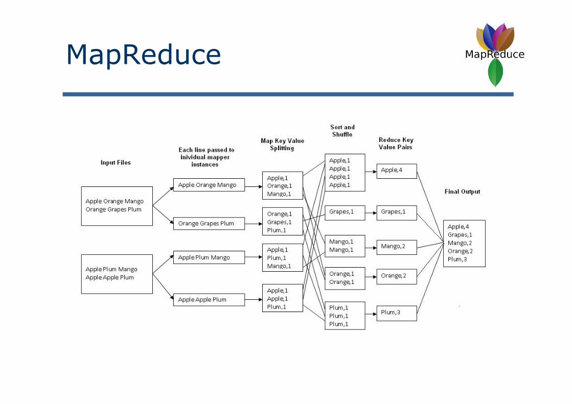
MapReduce
MapReduce is a popular approach to deal with Big Data
Based on a key-value pair data structure
Two key operations:1. Map function: Process
independent data blocks and outputs summary information
2. Reduce function: Further process previous independent results
J. Dean, S. Ghemawat, MapReduce: Simplified data processing on large clusters,Communications of the ACM 51 (1) (2008) 107-113.
input inputinputinput
mapmap map map
Shuffling: group values by keys
reduce reduce reduce
output output output
map (k, v) → list (k’, v’)reduce (k’, list(v’)) → v’’
(k , v)(k , v)(k , v) (k , v)
(k’, v’)(k’, v’)(k’, v’)(k’, v’)
k’, list(v’)k’, list(v’)k’, list(v’)
v’’v’’v’’

MapReduce
Blocks/fragments
Intermediary Files
Output Files
The key of a MapReduce data partitioning approach is usually on the reduce phase
MapReduce workflow
MapReduce

Runs on large commodity clusters: 10s to 10,000s of machines
Processes many terabytes of data Easy to use since run-time complexity hidden from
the users Cost-efficiency:
Commodity nodes (cheap, but unreliable) Commodity network Automatic fault-tolerance (fewer administrators) Easy to use (fewer programmers)
Experience
MapReduce
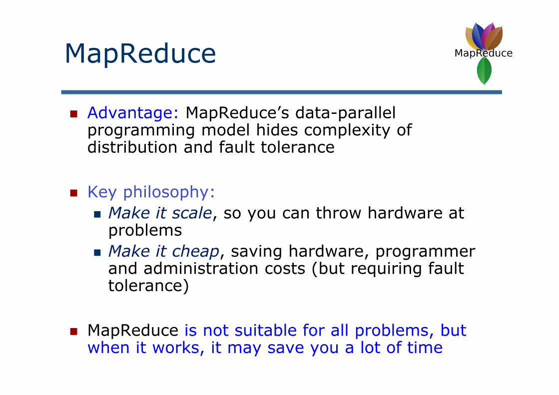
Advantage: MapReduce’s data-parallel programming model hides complexity of distribution and fault tolerance
Key philosophy: Make it scale, so you can throw hardware at
problems Make it cheap, saving hardware, programmer
and administration costs (but requiring fault tolerance)
MapReduce is not suitable for all problems, but when it works, it may save you a lot of time
MapReduce

MapReduce. Hadoop
Hadoop is an open source
implementation of MapReduce
computational paradigm
http://hadoop.apache.org/
Created by Doug Cutting (chairman of board of directors of the Apache Software Foundation, 2010)

Map ReduceLayer
HDFSLayer
Task tracker
Jobtracker
Task tracker
Namenode
Data nodeData node
Data node
http://hadoop.apache.org/
Apache Hadoop is an open-source software framework that supports data-intensive distributed applications, licensed under the Apache v2 license.
Created by Doug Cutting (chairman of board of directors of the Apache Software Foundation, 2010)
Hadoop implements the computational paradigm named
MapReduce
Hadoop

Hadoop
Amazon Elastic Compute Cloud (Amazon EC2)http://aws.amazon.com/es/ec2/
Windows Azurehttp://www.windowsazure.com/
How do I access to a Hadoop platform?
Cloud Platform with Hadoop installation
Cluster InstalationExample ATLAS, SCI2S Research Group
Cluster ATLAS: 4 super servers from Super Micro Computer Inc. (4 nodes per server) The features of each node are:
Microprocessors: 2 x Intel Xeon E5-2620 (6 cores/12 threads, 2 GHz, 15 MB Cache)
RAM 64 GB DDR3 ECC 1600MHz, Registered 1 HDD SATA 1TB, 3Gb/s; (system) 1 HDD SATA 2TB, 3Gb/s; (distributed file system)

July 2008 - Hadoop Wins Terabyte Sort BenchmarkOne of Yahoo's Hadoop clusters sorted 1 terabyte of data in 209 seconds, which beat the previous record of 297 seconds in the annual general purpose (Daytona) terabyte short bechmark. This is the first time that either a Java or an open source program has won.
http://developer.yahoo.com/blogs/hadoop/hadoop-sorts-petabyte-16-25-hours-terabyte-62-422.html
Hadoop birth

http://hadoop.apache.org/
The project
Recently: Apache Spark
Hadoop Ecosystem

The following malfunctions types of algorithms are examples where MapReduce:Iterative Graph Algorithms: PageRankGradient DescentExpectation Maximization
‘‘If all you have is a hammer, then everything looks like a nail.’’
MapReduce: Limitations
Pregel (Google)

On the limitations of Hadoop. New platformsGIRAPH (APACHE Project)(http://giraph.apache.org/)Iterative graphs
GPS - A Graph Processing System, (Stanford) http://infolab.stanford.edu/gps/Amazon's EC2
Distributed GraphLab (Carnegie Mellon Univ.)
https://github.com/graphlab-code/graphlabAmazon's EC2
HaLoop (University of Washington)
http://clue.cs.washington.edu/node/14 http://code.google.com/p/haloop/Amazon’s EC2
Twister (Indiana University)http://www.iterativemapreduce.org/
PrIter (University of Massachusetts. Amherst, Northeastern University-China)
http://code.google.com/p/priter/Amazon EC2 cloud
GPU based platformsMarsGrex
Spark (UC Berkeley)(100 times more efficient than Hadoop,
including iterative algorithms, according to creators) http://spark.incubator.apache.org/research.html
Hadoop

35
MapReduce
Enrique AlfonsecaGoogle Research Zurich
More than 10000 applications in Google

Hadoop Ecosystem
Hadoop Evolution
Bibliografía: A. Fernandez, S. Río, V. López, A. Bawakid, M.J. del Jesus, J.M. Benítez, F. Herrera, Big Datawith Cloud Computing: An Insight on the Computing Environment, MapReduce and ProgrammingFrameworks. WIREs Data Mining and Knowledge Discovery 4:5 (2014) 380-409
MapReduce Limitations. Graph algorithms (Page Rank, Google), iterative algorithms.

Apache Spark

InMemoryHDFS Hadoop + SPARK
EcosystemApache Spark
Future version of Mahout for Spark
Apache Spark: InMemory

Spark birth
http://databricks.com/blog/2014/10/10/spark-petabyte-sort.html
Using Spark on 206 EC2 nodes, we completed the benchmark in 23 minutes. This means that Spark sorted the same data 3X faster using 10X fewer machines. All the sorting took place on disk (HDFS), without using Spark’s in-memory cache.
October 10, 2014

Spark birth
http://sortbenchmark.org/

41
Outline
Big Data. Big Data Science. Data Preprocessing
Why Big Data? MapReduce Paradigm. Hadoop Ecosystem
Big Data Classification: Learning algorithms
Data Preprocessing
Big data Preprocessing
Imbalanced Big Data Classification: Data preprocessing
Challenges and Final Comments

Generation 1st Generation
2nd Generation 3nd Generation
Examples SAS, R, Weka, SPSS, KEEL
Mahout, Pentaho, Cascading
Spark, Haloop, GraphLab,Pregel, Giraph, ML overStorm
Scalability Vertical Horizontal (overHadoop)
Horizontal (BeyondHadoop)
AlgorithmsAvailable
Hugecollection of algorithms
Small subset: sequentiallogistic regression, linear SVMs, StochasticGradient Decendent, k-means clustsering, Random forest, etc.
Much wider: CGD, ALS, collaborative filtering, kernel SVM, matrixfactorization, Gibbssampling, etc.
AlgorithmsNotAvailable
Practicallynothing
Vast no.: Kernel SVMs, Multivariate LogisticRegression, ConjugateGradient Descendent, ALS, etc.
Multivariate logisticregression in general form, k-means clustering, etc. –Work in progress to expandthe set of availablealgorithms
Fault-Tolerance
Single pointof failure
Most tools are FT, as they are built on top of Hadoop
FT: HaLoop, SparkNot FT: Pregel, GraphLab, Giraph
Classification

43
Classification
Mahout
MLlib
https://spark.apache.org/mllib/

44
Classification

http://mahout.apache.org/
Classification: Mahout

Classification: Mahout
Four great application areas
Clustering
Recommendation Systems
Classification
Association

Classification: RF
Case of Study: Random Forest forKddCup’99

48
Classification: RF
The RF Mahout Partial implementation: is an algorithm that builds multiple trees for different portions of the data. Two phases:
Building phase Classification phase
Case of Study: Random Forest forKddCup’99

Classification: RF
Case of Study: Random Forest forKddCup’99
Class InstanceNumber
normal 972.781DOS 3.883.370PRB 41.102R2L 1.126U2R 52

Classification: RF
Class InstanceNumber
normal 972.781DOS 3.883.370PRB 41.102R2L 1.126U2R 52
Case of Study: Random Forest forKddCup’99
Cluster ATLAS: 16 nodes-Microprocessors: 2 x Intel E5-2620 (6 cores/12 threads, 2 GHz)- RAM 64 GB DDR3 ECC 1600MHz- Mahout version 0.8

51
Outline
Big Data. Big Data Science. Data Preprocessing
Why Big Data? MapReduce Paradigm. Hadoop Ecosystem
Big Data Classification: Learning algorithms
Data Preprocessing
Big Data Preprocessing
Imbalanced Big Data Classification: Data preprocessing
Challenges and Final Comments

Data Science
Big Data
Model buildingPredictive and descriptiveAnalytics
Data Preprocessing
Data Preprocessing

1. Introduction. Data Preprocessing2. Integration, Cleaning and Transformations3. Imperfect Data4. Data Reduction5. Final Remarks
Data PreprocessingBibliography:
S. García, J. Luengo, F. HerreraData Preprocessing in Data MiningSpringer, January 2015
Websites: http://sci2s.ugr.es/books/data-preprocessinghttp://www.springer.com/us/book/9783319102467

Data Preprocessing
1. Introduction. Data Preprocessing2. Integration, Cleaning and Transformations3. Imperfect Data4. Data Reduction5. Final Remarks

D. Pyle, 1999, pp. 90:
“The fundamental purpose of data preparation is to manipulate and transform raw data so that the information content enfolded in the data set can be exposed, or made more easily accesible.”
Dorian PyleData Preparation for Data Mining Morgan Kaufmann Publishers, 1999
INTRODUCTION

Data Preprocessing
1. Real data could be dirty and could drive to the extraction of useless patterns/rules.
This is mainly due to:
Incomplete data: lacking attribute values, …Data with noise: containing errors or outliersInconsistent data (including discrepancies)
Importance of Data Preprocessing

2. Data preprocessing can generate a smaller data set than the original, which allows us to improve the efficiency in the Data Mining process.
This performing includes Data Reduction techniques:Feature selection, sampling or instance selection, discretization.
Data PreprocessingImportance of Data Preprocessing

3. No quality data, no quality mining results!
Data preprocessing techniques generate “quality data”, driving us to obtain “quality patterns/rules”.
Data PreprocessingImportance of Data Preprocessing
Quality decisions must be based on quality data!

Data preprocessing spends a very important part of the total time in a data mining process.
Data Preprocessing

60
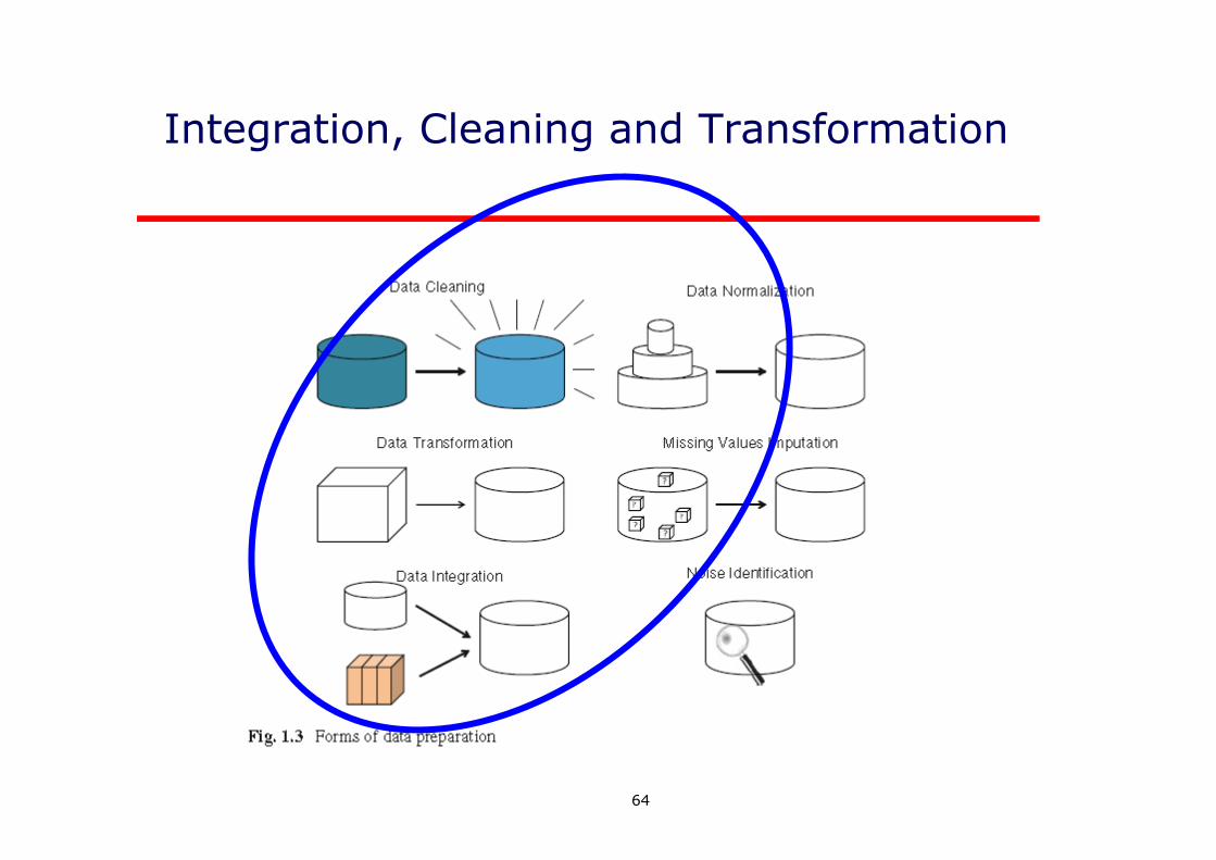
Real databases usually contain noisy data, missing data, and inconsistent data, …
1. Data integration. Fusion of multiple sources in a Data Warehousing.
2. Data cleaning. Removal of noise and inconsistencies.
3. Missing values imputation.
4. Data Transformation.
5. Data reduction.
Data PreprocessingWhat is included in data preprocessing?
Major Tasks in Data Preprocessing

61
Data PreprocessingWhat is included in data preprocessing?

62
Data PreprocessingWhat is included in data preprocessing?
Data Preprocessing
1. Introduction. Data Preprocessing2. Integration, Cleaning and Transformations3. Imperfect Data4. Data Reduction5. Final Remarks
64
Integration, Cleaning and Transformation

65
Data Integration
Obtain data from different information sources.
Address problems of codification and representation.
Integrate data from different tables to produce homogeneous information, ...
Data WarehouseServer Database 1
Extraction, aggregation ..
Database 2

66
Different scales: Salary in dollars versus euros (€)
Derivative attributes: Mensual salary versus annual salary
item Salary/month 1 5000 2 2400 3 3000
item Salary 6 50,000 7 100,000 8 40,000
Examples
Data Integration

67
Data Cleaning
Objetictives: • Fix inconsistencies• Fill/impute missing values, • Smooth noisy data, • Identify or remove outliers …
Some Data Mining algorithms have proper methods to deal with incomplete or noisy data. But in general, these methods are not very robust. It is usual to perform a data cleaning previously to their application.
Bibliography: W. Kim, B. Choi, E.-D. Hong, S.-K. KimA taxonomy of dirty data.Data Mining and Knowledge Discovery 7, 81-99, 2003.

68
Data Cleaning
Original Data
Clean Data
000000000130.06.19971979-10-3080145722 #000310 111000301.01.000100000000004 0000000000000.000000000000000.000000000000000.000000000000000.000000000000000.000000000000000.000000000000000. 000000000000000.000000000000000.0000000...… 000000000000000.000000000000000.000000000000000.000000000000000.000000000000000.000000000000000.000000000000000.000000000000000.000000000000000.000000000000000.000000000000000.000000000000000.000000000000000.000000000000000.000000000000000.000000000000000.000000000000000.000000000000000.000000000000000.000000000000000.000000000000000.000000000000000.00 0000000000300.00 0000000000300.00
0000000001,199706,1979.833,8014,5722 , ,#000310 …. ,111,03,000101,0,04,0,0,0,0,0,0,0,0,0,0,0,0,0,0,0,0,0,0,0,0,0,0,0,0,0,0,0,0,0,0,0,0,0,0,0,0,0,0,0,0,0,0,0,0,0,0300,0,0,0,0,0,0,0,0,0,0,0,0,0,0,0,0,0,0,0,0,0,0,0,0,0,0,0,0,0,0,0,0,0,0,0,0,0,0,0,0,0,0,0,0,0,0,0,0300,0300.00
Data cleaning: Example

69
Data Cleaning
Age=“42” Birth Date=“03/07/1997”
Data Cleaning: Inconsistent data

70
Data transformation Objective: To transform data in the best
way possible to the application of Data Mining algorithms.
Some typical operations:• Aggregation. i.e. Sum of the totality of month sales in an
unique attribute called anual sales,…• Data generalization. It is to obtain higher degrees of data from
the currently available, by using concept hierarchies. streets cities Numerical age {young, adult, half-age, old}
• Normalization: Change the range [-1,1] or [0,1].
• Lineal transformations, quadratic, polinominal, …
Bibliography:T. Y. Lin. Attribute Transformation for Data Mining I: TheoreticalExplorations. International Journal of Intelligent Systems 17, 213-222, 2002.
71
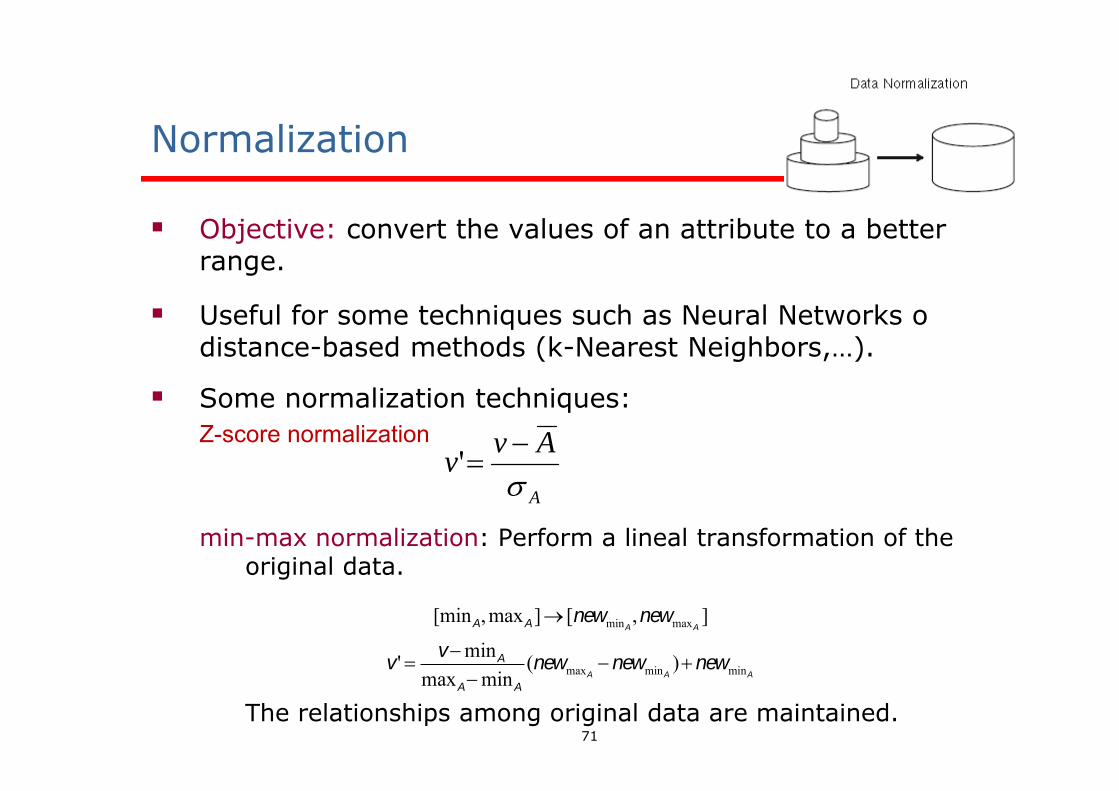
Normalization
Objective: convert the values of an attribute to a better range.
Useful for some techniques such as Neural Networks o distance-based methods (k-Nearest Neighbors,…).
Some normalization techniques:Z-score normalization
min-max normalization: Perform a lineal transformation of the original data.
The relationships among original data are maintained.
[minA, maxA] [newminA,newmaxA
]
v' vminA
maxAminA
(newmaxAnewminA
)newminA
A
Avv
'

Data Preprocessing
1. Introduction. Data Preprocessing2. Integration, Cleaning and Transformations3. Imperfect Data4. Data Reduction5. Final Remarks

73
Imperfect data

74
Missing values

75
Missing values
It could be used the next choices, although some of them may skew the data:
Ignore the tuple. It is usually used when the variable to classify has no value.
Use a global constant for the replacement. I.e. “unknown”,”?”,…
Fill tuples by means of mean/deviation of the rest of the tuples.
Fill tuples by means of mean/deviation of the rest of the tuples belonging to the same class.
Impute with the most probable value. For this, some technique of inference could be used, i.e., bayesian or decision trees.

76
Missing values
15 methodshttp://www.keel.es/

77
Missing values

78
Missing values
Bibliography:WEBSITE: http://sci2s.ugr.es/MVDM/
J. Luengo, S. García, F. Herrera, A Study on the Use of Imputation Methods for Experimentation with Radial Basis Function Network Classifiers Handling Missing Attribute Values: The good synergy between RBFs and EventCovering method. Neural Networks, doi:10.1016/j.neunet.2009.11.014, 23(3) (2010) 406-418.
S. García, F. Herrera, On the choice of the best imputation methods for missing values considering three groups of classification methods. Knowledge and Information Systems 32:1 (2012) 77-108, doi:10.1007/s10115-011-0424-2
79
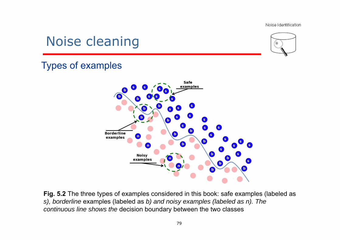
Noise cleaning
Types of examples
Fig. 5.2 The three types of examples considered in this book: safe examples (labeled as s), borderline examples (labeled as b) and noisy examples (labeled as n). The continuous line shows the decision boundary between the two classes

80
Noise cleaning
Fig. 5.1 Examples of the interaction between classes: a) small disjuncts and b) overlapping between classes

81
The three noise filters mentioned next, which are the most-
known, use a voting scheme to determine what cases have to be
removed from the training set:
Ensemble Filter (EF) Cross-Validated Committees Filter Iterative-Partitioning Filter
Noise cleaning
Use of noise filtering techniques in classification

Ensemble Filter (EF)• C.E. Brodley, M.A. Friedl. Identifying Mislabeled Training Data. Journal of Artificial Intelligence Research 11
(1999) 131‐167.• Different learning algorithm (C4.5, 1‐NN and LDA) are used to create classifiers in several subsets of the
training data that serve as noise filters for the training sets.• Two main steps:1. For each learning algorithm, a k‐fold cross‐validation is used to tag each training example as correct
(prediction = training data label) or mislabeled (prediction ≠ training data label).2. A voting scheme is used to identify the final set of noisy examples.
• Consensus voting: it removes an example if it is misclassified by all the classifiers.• Majority voting: it removes an instance if it is misclassified by more than half of the classifiers.
Training Data
Classifier #1 Classifier #2 Classifier #m
Noisy examples
( / )Classification #1
(correct/mislabeled) ( / )Classification #2
(correct/mislabeled) ( / )Classification #m
(correct/mislabeled)
Voting scheme(consensus or majority)

Ensemble Filter (EF)

Cross‐Validated Committees Filter (CVCF)• S. Verbaeten, A.V. Assche. Ensemble methods for noise elimination in
classification problems. 4th International Workshop on Multiple Classifier Systems (MCS 2003). LNCS 2709, Springer 2003, Guilford (UK, 2003) 317‐325.
• CVCF is similar to EF two main differences:
1. The same learning algorithm (C4.5) is used to create classifiers in several subsets of the training data.
The authors of CVCF place special emphasis on using ensembles of decision trees such as C4.5 because they work well as a filter for noisy data.
2. Each classifier built with the k‐fold cross‐validation is used to tag ALL the training examples (not only the test set) as correct (prediction = training data label) or mislabeled (prediction ≠ training data label).

Iterative Partitioning Filter (IPF)• T.M. Khoshgoftaar, P. Rebours. Improving software quality prediction by noise filtering
techniques. Journal of Computer Science and Technology 22 (2007) 387‐396.• IPF removes noisy data in multiple iterations using CVCF until a stopping criterion is reached.• The iterative process stops if, for a number of consecutive iterations, the number of noisy
examples in each iteration is less than a percentage of the size of the training dataset.
Training Data
CVCF Filter
Current Training Data without Noisyexamples identified by CVCF
Current Training Data
Final Noisy examples
STOP?NO
YES

INFFC: An iterative class noise filter based on the fusion of classifiers with noise sensitivity control

INFFC: An iterative class noise filter based on the fusion of classifiers with noise sensitivity control
http://www.sciencedirect.com/science/article/pii/S156625351500038X

88
Noise cleaning
http://www.keel.es/
Bibliography:WEBSITE: http://sci2s.ugr.es/noisydata/

Data Preprocessing
1. Introduction. Data Preprocessing2. Integration, Cleaning and Transformations3. Imperfect Data4. Data Reduction5. Final Remarks

90
Data Reduction

Feature Selection
The problem of Feature Subset Selection (FSS) consists of
finding a subset of the attributes/features/variables of the
data set that optimizes the probability of success in the
subsequent data mining taks.

1 2 3 4 5 6 7 8 9 10 11 12 13 14 15 16A 0 0 0 0 0 0 0 0 1 1 1 1 1 1 1 1B 0 0 0 0 1 1 1 1 0 0 0 0 1 1 1 1C 0 0 1 1 0 0 1 1 0 0 1 1 0 0 1 1D 0 1 0 1 0 1 0 1 0 1 0 1 0 1 0 1E 0 1 0 0 0 1 1 0 1 1 0 0 0 0 1 0F 1 1 1 0 1 1 0 0 1 0 1 0 0 1 0 0
Var. 5Var. 1. Var. 13
Feature Selection

Feature Selection
The problem of Feature Subset Selection (FSS) consists of finding a subset of the attributes/features/variables of the data set that optimizes the probability of success in the subsequent data mining taks.
Why is feature selection necessary?
More attributes do not mean more success in the data mining process.
Working with less attributes reduces the complexity of the problem and the running time.
With less attributes, the generalization capability increases. The values for certain attributes may be difficult and costly
to obtain.

Feature Selection
The outcome of FS would be: Less data algorithms couls learn quickly
Higher accuracy the algorithm better generalizes
Simpler results easier to understand them
FS has as extension the extraction and construction of attributes.

Feature Selection
Complete Set of
Features
Empty Set of
Features
Fig. 7.1 Search space for FS

{}
{1} {2} {3} {4}
{1}{3} {2,3} {1,4} {2,4}{1,2} {3,4}
{1,2,3} {1,2,4} {1,3,4} {2,3,4}
{1,2,3,4}
It can be considered as a search problem
Feature Selection

(SG) Subset
generation
(EC) EvaluationFunction
SelectedSubsetStop
criteria
no
feature
subset
Targetdata
Yes
Process
Feature Selection

Feature Selection
Goal functions: There are two different approaches
Filter. The goal function evaluates the subsets basing on the information they contain. Measures of class separability, statistical dependences, information theory,… are used as the goal function.
Wrapper. The goal function consists of applying the same learning technique that will be used later over the data resulted from the selection of the features. The returned value usually is the accuracy rate of the constructed classifier.

Feature SelectionProcess
Fig. 7.2 A filter model for FS

Feature Selection
Filtering measures Separability measures. They estimate the separability among
classes: euclidean, Mahalanobis,… I.e. In a two-class problem, a FS process based on this kind of measures
determined that X is bettern than Y if X induces a greater difference than Y between the two prior conditional probabilities between the classes.
Correlation. Good subset will be those correlated with the class variable
where ρic is the coefficient of correlation between the variable Xi and the label c of the class (C) and ρij is the correlation coefficient between Xiand Xj
M
i
M
ijij
M
iic
MXXf
1 1
11 ),...,(

Feature Selection
Information theory based measures Correlation only can estimate lineal dependences. A more powerful
method is the mutual information I(X1,…,M; C)
where H represents the entropy and ωc the c-th label of the class C Mutual information measures the quantity of uncertainty that
decreases in the class C when the values of the vector X1…M are known. Due to the complexity of the computation of I, it is usual to use
heurisctics rules
with β=0.5, as example.
dxPXP
XPXP
XCHCHCXIXfC
c X cM
cMcM
MMM
M
1 ...1
...1...1
,...,1,...,1,...,1
,...,1)()(
),(log),(
)()();()(
M
i
M
i
M
ijjiiM XXICXIXf
1 1 1...1 );();()(

Feature Selection Consistency measures
The three previous groups of measures try to find those features than could, maximally, predict the class better than the remain.
• This approach cannot distinguish between two attributes that are equally appropriate, it does not detect redundant features.
Consistency measures try to find a minimum number of features that are able to separate the classes in the same way that the original data set does.
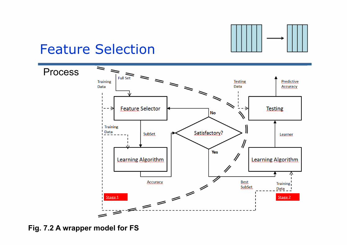
Feature SelectionProcess
Fig. 7.2 A wrapper model for FS

Feature SelectionProcess
Fig. 7.2 A filter model for FS

Feature Selection
Advantages
Wrappers: Accuracy: generally, they are more accurate than filters,
due to the interaction between the classifier used in the goal function and the training data set.
Generalization capability: they pose capacity to avoid overfitting due to validation techniques employed.
Filters: Fast: They usually compute frequencies, much quicker than
training a classifier. Generality: Due to they evaluate instrinsic properties of the
data and not their interaction with a classifier, they can be used in any problem.

Feature Selection
Drawbacks
Wrappers: Very costly: for each evaluation, it is required to learn and
validate a model. It is prohibitive to complex classifiers. Ad-hoc solutions: The solutions are skewed towards the
used classifier.
Filters: Trend to include many variables: Normally, it is due to
the fact that there are monotone features in the goal function used.
• The use should set the threshold to stop.

Feature Selection
4. According to outcome:
Ranking
Subset of features
1. According to evaluation:
filter
wrapper
2. Class availability:
Supervised
Unsupervised
3. According to the search:
Complete O(2N)Heurístic O(N2)Random ??
Categories

Feature Selection
Input: x attributes – U evaluation criterion
Subset = {}
Repeat
Sk = generateSubset(x)
if improvement(S, Sk,U)
Subset = Sk
Until StopCriterion()
Output: List, of the most relevant atts.
Algorithms for getting subset of featuresThey return a subset of attributes optimized according to an evaluation criterion.
Feature Selection
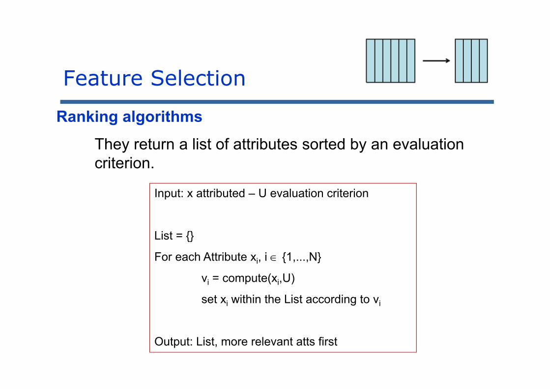
Input: x attributed – U evaluation criterion
List = {}
For each Attribute xi, i {1,...,N}
vi = compute(xi,U)
set xi within the List according to vi
Output: List, more relevant atts first
They return a list of attributes sorted by an evaluation criterion.
Ranking algorithms

Feature Selection
Ranking algorithms
Attributes A1 A2 A3 A4 A5 A6 A7 A8 A9
Ranking A5 A7 A4 A3 A1 A8 A6 A2 A9
A5 A7 A4 A3 A1 A8 (6 attributes)

Feature Selection
Some relevant algorithms:
Focus algorithm. Consistency measure for forward search Mutual Information based Features Selection (MIFS). mRMR: Minimum Redundancy Maximum Relevance Las Vegas Filter (LVF) Las Vegas Wrapper (LVW) Relief Algorithm

Instance selection try to choose the examples which are relevant to an application, achieving the maximum performance. The outcome of IS would be:
Less data algorithms learn quicker
Higher accuracy the algorithm better generalizes
Simpler results easier to understand them
IS has as extension the generation of instances (prototype generation)
Instance Selection

Different size examples
8000 points 2000 points 500 points
Instance Selection
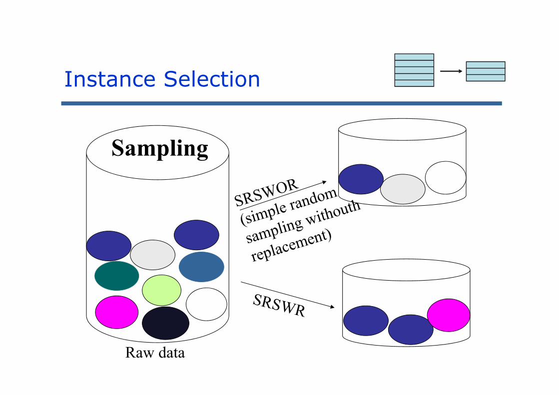
Sampling
Raw data
Instance Selection

SamplingRaw Data Simple reduction
Instance Selection

Instance Selection
Training Data Set
(TR)
Test Data Set
(TS)
InstancesSelected (S)
PrototypeSelectionAlgorithm
Instance-basedClassifier
Fig. 8.1 PS process

Prototype Selection (instance-based learning)
Properties:
Direction of the search: Incremental, decremental,
batch, hybrid or fixed.
Selection type: Condensation, Edition, Hybrid.
Evaluation type: Filter or wrapper.
Instance Selection

Instance Selection

Classical algorithm of condensation: Condensed Nearest Neighbor (CNN) Incremental It only inserts the misclassified instances in the new subsets. Dependant on the order of presentation. It only retains borderline examples.
A pair of classical algorithms:
Instance Selection

Classical algorithm for Edition: Edited Nearest Neighbor (ENN) Batch It removes those instances which are wrongly classified by using a k-nearest
neighbor scheme (k = 3, 5 or 9). It “smooths” the borders among classes, but also retains the rest of points.
A pair of classical algorithms:
Instance Selection

Graphical illustrations (Condensation vs Edition):
Banana data set with 5,300 instances and two classes. Obtained subset with CNN and AllKNN (iterative application of ENN with k=3, 5 y 7).
Instance Selection

Graphical illustrations:
RMHC is an adaptive sampling technique based on local search with a fixed final rate of retention.
DROP3 is the most-known hybrid technique very use for kNN.SSMA is an evolutionary approach based on memetic algorithms..
Instance Selection

Instance Selection
Training Set Selection

Kdd Cup’99. Strata Number: 100No.
Rules%
ReductionC4.5
%Ac Trn %Ac TestC4.5 252 99.97% 99.94%Cnn Strat 83 81.61% 98.48% 96.43%Drop1 Strat 3 99.97% 38.63% 34.97%Drop2 Strat 82 76.66% 81.40% 76.58%Drop3 Strat 49 56.74% 77.02% 75.38%Ib2 Strat 48 82.01% 95.81% 95.05%Ib3 Strat 74 78.92% 99.13% 96.77%Icf Strat 68 23.62% 99.98% 99.53%CHC Strat 9 99.68% 98.97% 97.53%
Example Instance Selection and Decision Tree modeling
Bibliography: J.R. Cano, F. Herrera, M. Lozano, Evolutionary Stratified Training Set Selection for Extracting Classification Rules with Trade-off Precision-Interpretability. Data and Knowledge Engineering 60 (2007) 90-108, doi:10.1016/j.datak.2006.01.008.

S. García, J. Derrac, J.R. Cano and F. Herrera,Prototype Selection for Nearest Neighbor Classification: Taxonomy and Empirical Study.IEEE Transactions on Pattern Analysis and Machine Intelligence 34:3 (2012) 417-435 doi:10.1109/TPAMI.2011.142
S. García, J. Luengo, F. Herrera. Data Preprocessing in Data Mining, Springer, 15, 2015
WEBSITE: http://sci2s.ugr.es/pr/index.phpBibliography:
Instance Selection
Source Codes (Java):

Discretization
Discrete values are very useful in Data Mining.
They represent more concise information, they are easier to understand and closer to the representation of knowledge.
The discretization is focused on the transformation of continuous values with an order among in nominal/categorical values without ordering. It is also a quantification of numerical attributes.
Nominal values are within a finite domain, so they are also considered as a data reduction technique.
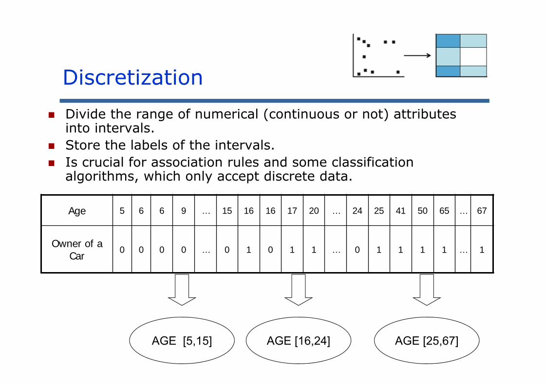
Divide the range of numerical (continuous or not) attributes into intervals.
Store the labels of the intervals. Is crucial for association rules and some classification
algorithms, which only accept discrete data.
Age 5 6 6 9 … 15 16 16 17 20 … 24 25 41 50 65 … 67
Owner of a Car 0 0 0 0 … 0 1 0 1 1 … 0 1 1 1 1 … 1
AGE [5,15] AGE [16,24] AGE [25,67]
Discretization

Stages in the discretization process
Discretization

Discretization Discretization has been developed in several lines
according to the neccesities:
Supervised vs. unsupervised: Whether or not they consider the objective (class) attributes.
Dinamical vs. Static: Simultaneously when the model is built or not.
Local vs. Global: Whether they consider a subset of the instances or all of them.
Top-down vs. Bottom-up: Whether they start with an empty list of cut points (adding new ones) or with all the possible cut points (merging them).
Direct vs. Incremental: They make decisions all together or one by one.

Unsupervised algorithms: • Equal width• Equal frequency• Clustering …..
Supervised algorithms:
• Entropy based [Fayyad & Irani 93 and others] [Fayyad & Irani 93] U.M. Fayyad and K.B. Irani. Multi-interval discretization of continuous-valued attributes for classification learning. Proc. 13th Int. Joint Conf. AI (IJCAI-93), 1022-1027. Chamberry, France, Aug./ Sep. 1993.
• Chi-square [Kerber 92] [Kerber 92] R. Kerber. ChiMerge: Discretization of numeric attributes. Proc. 10th Nat. Conf. AAAI, 123-128. 1992.
• … (lots of proposals)
Discretization
Bibliography: S. García, J. Luengo, José A. Sáez, V. López, F. Herrera, A Survey of Discretization Techniques: Taxonomy and Empirical Analysis in Supervised Learning. IEEE Transactions on Knowledge and Data Engineering 25:4 (2013) 734-750, doi: 10.1109/TKDE.2012.35.
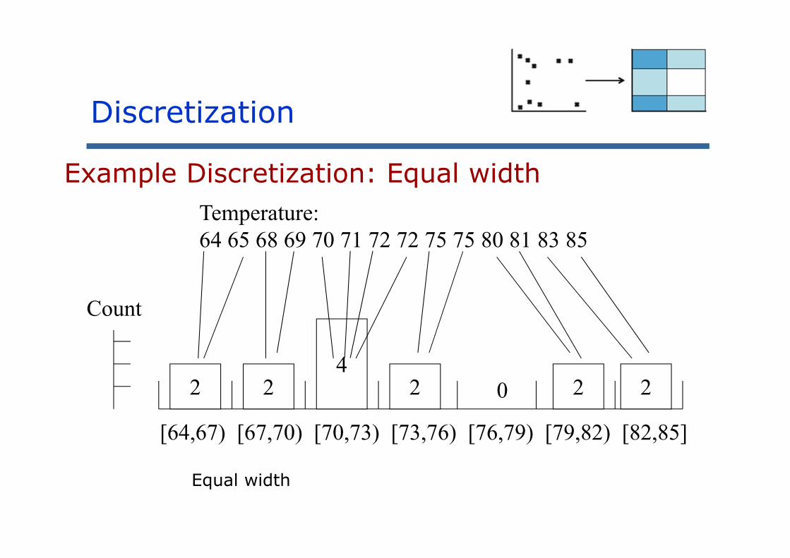
Example Discretization: Equal width
Equal width
[64,67) [67,70) [70,73) [73,76) [76,79) [79,82) [82,85]
Temperature:64 65 68 69 70 71 72 72 75 75 80 81 83 85
2 2
Count
42 2 20
Discretization

Example discretization: Equal frequency
Equal frequency (height) = 4, except for the last box
[64 .. .. .. .. 69] [70 .. 72] [73 .. .. .. .. .. .. .. .. 81] [83 .. 85]
Temperature64 65 68 69 70 71 72 72 75 75 80 81 83 85
4
Count
4 42
Discretization

Discretization
Which discretizer will be the best?.
As usual, it will depend on the application, user requirements, etc.
Evaluation ways:
Total number of intervals Number of inconsistencies Predictive accuracy rate of classifiers

Data Preprocessing
1. Introduction. Data Preprocessing2. Integration, Cleaning and Transformations3. Imperfect Data4. Data Reduction5. Final Remarks

Final Remarks
Data preprocessing is a necessity when we work with real applications.
Data Pre-
processingPatterns
Extraction
Interpretabilityof
results
Raw data Knowledge

Final Remarks
Real data could be dirty and could drive to the extraction of useless patterns/rules.
Data preprocessing can generate a smaller data set than the original, which allows us to improve the efficiency in the Data
Mining process.
No quality data, no quality mining results!
Quality decisions must be based on quality data!

Data Preprocessing Advantage: Data preprocessing
allows us to apply Learning/Data Mining algorithms easier
and quicker, obtaining more quality models/patterns in terms
of accuracy and/or interpretability.
Final Remarks

Data Preprocessing Advantage: Data preprocessing allows us to applyLearning/Data Mining algorithms easier and quicker, obtaining more qualitymodels/patterns in terms of accuracy and/or interpretability.
Final Remarks
A drawback: Data preprocessing is not a structured area
with a specific methodology for understanding the suitability
of preprocessing algorithms for managing a new problems.
Every problem can need a different preprocessing process, using different tools. The design of automatic processes of use of the different
stages/techniques is one of the data mining challenges.

Final Remarks
Website including slides, material, links …(under preparation)
http://sci2s.ugr.es/books/data-preprocessing

Outline
Big Data. Big Data Science. Data Preprocessing
Why Big Data? MapReduce Paradigm. Hadoop Ecosystem
Big Data Classification: Learning algorithms
Data Preprocessing
Big Data Preprocessing
Imbalanced Big Data Classification: Data preprocessing
Challenges and Final Comments

Big Data Preprocessing
Preprocessing for Big Data analytics
Tasks to discuss:
1. Scalability of the proposals (Algorithms redesign!!)
2. Reduce phase: How must we combine the output of the maps? (Fundamental phase to use MapReduce for Big Data Preprocessing!!)
1. Appearance of small disjuncts with the MapReduce data fragmentation. This problem is basically associated to imbalanced classification: Lack of Data/lack of density

Density: Lack of data
The lack of density in the training data may also cause the introduction of small disjuncts.
It becomes very hard for the learning algorithm to obtain a model that is able to perform a good generalization when there is not enough data that represents the boundaries of the problem and, what it is also most significant, when the concentration of minority examples is so low that they can be simply treated as noise.
Appearance of small disjuncts with the MapReduce data fragmentation

Big Data PreprocessingBird's eye view
9 cases of study 10 chapters giving a quick glance on Machine Learning with Spakr

Big Data PreprocessingBird's eye view
A short introduction todata preparation with Spark – Chapter 3

ChiSqSelectorChiSqSelector stands for Chi-Squared feature selection. It operates on labeled data with categorical features. ChiSqSelector orders features based on a Chi-Squared test of independence from the class, and then filters (selects) the top features which are most closely related to the label.
Model FittingChiSqSelector has the following parameter in the constructor:• numTopFeatures number of top features that the selector will select (filter).
Big Data Preprocessinghttps://spark.apache.org/docs/latest/mllib-guide.htmlBird's eye view

Big Data PreprocessingBird's eye view http://sci2s.ugr.es/BigData

Big Data PreprocessingBird's eye view http://sci2s.ugr.es/BigData

Big Data PreprocessingBird's eye view
Feature Selection
MapReduce based Evolutionary Feature Selection
https://github.com/triguero/MR-EFS
This repository includes the MapReduce implementations used in [1]. This implementation is based on Apache Mahout 0.8 library. The Apache Mahout (http://mahout.apache.org/) project's goal is to build an environment for quickly creating scalable performant machine learning applications.
[1] D. Peralta, S. Del Río, S. Ramírez-Gallego, I. Triguero, J.M. Benítez, F. Herrera. Evolutionary Feature Selection for Big Data Classification: A MapReduce Approach.Mathematical Problems in Engineering, In press, 2015.
http://sci2s.ugr.es/BigData

Big Data PreprocessingBird's eye view
Feature Selection
An Information Theoretic Feature Selection Framework for Spark
https://github.com/sramirez/spark-infotheoretic-feature-selectionhttp://spark-packages.org/package/sramirez/spark-infotheoretic-feature-selection
This package contains a generic implementation of greedy Information Theoretic Feature Selection (FS) methods. The implementation is based on the common theoretic framework presented by Gavin Brown. Implementations of mRMR, InfoGain, JMI and other commonly used FS filters are provided
http://sci2s.ugr.es/BigData

Big Data PreprocessingBird's eye view
Feature Selection
Fast-mRMR: an optimal implementation of minimum Redundancy Maximum Relevance algorithm
https://github.com/sramirez/fast-mRMR
This is an improved implementation of the classical feature selection method: minimum Redundancy and Maximum Relevance (mRMR); presented by Peng in (Hanchuan Peng, Fuhui Long, and Chris Ding "Feature selection based on mutual information: criteria of max-dependency, max-relevance, and min-redundancy," IEEE Transactions on Pattern Analysis and Machine Intelligence, Vol. 27, No. 8, pp.1226-1238, 2005). This includes several optimizations such as: cache marginal probabilities, accumulation of redundancy (greedy approach) and a data-access by columns.
http://sci2s.ugr.es/BigData
Fast-mRMR

Big Data PreprocessingBird's eye view
Feature Weighting
https://github.com/triguero/ROSEFW-RF
This project contains the code used in the ROSEFW-RF algorithm, including:
Evolutionary Feature WeightingRandomForestRandom Oversampling
I. Triguero, S. Río, V. López, J. Bacardit, J.M. Benítez, F. Herrera. ROSEFW-RF: The winner algorithm forthe ECBDL'14 Big Data Competition: An extremely imbalanced big data bioinformatics problem. Knowledge-Based Systems, in press. doi: 10.1016/j.knosys.2015.05.027
Feature weighting is a feature importance ranking technique where weights, not only ranks, are obtained. When successfully applied relevant features are attributed a high weight value, whereas irrelevant features are given a weight value close to zero. Feature weighting can be used not only to improve classification accuracy but also to discard features with weights below a certain threshold value and thereby increase the resource efficiency of the classifier.
http://sci2s.ugr.es/BigData

Big Data PreprocessingBird's eye view
Prototype Generation
MapReduce based Prototype Reduction
https://github.com/triguero/MRPR
This repository includes the MapReduce implementation proposed for Prototype Reduction for the algorithm MRPR.
I. Triguero, D. Peralta, J. Bacardit, S. García, F. Herrera. MRPR: A MapReduce Solution forPrototype Reduction in Big Data Classification. Neurocomputing 150 (2015), 331-345. doi: 10.1016/j.neucom.2014.04.078
http://sci2s.ugr.es/BigData

Big Data PreprocessingBird's eye view
DiscretizationDistributed Minimum Description Length Discretizer for Spark
https://github.com/sramirez/spark-MDLP-discretizationhttp://spark-packages.org/package/sramirez/spark-MDLP-discretization
Spark implementation of Fayyad's discretizer based on Minimum Description Length Principle (MDLP). Published in:
S. Ramírez-Gallego, S. García, H. Mouriño-Talin, D. Martínez-Rego, V. Bolón, A. Alonso-Betanzos, J.M. Benitez, F. Herrera. Distributed Entropy Minimization Discretizer for Big Data Analysis under Apache Spark. IEEE BigDataSE Conference, Helsinki, August, 2015.
http://sci2s.ugr.es/BigData

Big Data PreprocessingBird's eye view
Processing Imbalanced data setsImbalanced Data Preprocessing for Hadoop
https://github.com/saradelrio/hadoop-imbalanced-preprocessing
MapReduce implementations of random oversampling, random undersampling and ‘‘Synthetic Minority Oversampling TEchnique’’ (SMOTE) algorithms using Hadoop, used in:
S. Río, V. López, J.M. Benítez, F. Herrera, On the use of MapReduce for Imbalanced Big Data using Random Forest. Information Sciences 285 (2014) 112-137.
http://sci2s.ugr.es/BigData

Our approaches:
Big Data Preprocessing
https://github.com/sramirez
https://github.com/triguero https://github.com/saradelrio
Bird's eye view http://sci2s.ugr.es/BigData

• MRPR: A Combined MapReduce-Windowing Two-Level
Parallel Scheme for Evolutionary Prototype Generation
• MR-EFS: Evolutionary Feature Selection for Big Data
Classification: A MapReduce Approach
• Spark-ITFS: Filtering Feature Selection For Big Data
• Fast-mRMR: an optimal implementation of minimum
Redundancy Maximum Relevance algorithm
• Spark-MDLP: Distributed Entropy Minimization Discretizer for
Big Data Analysis under Apache Spark
Big Data Preprocessing
Describing some Approaches:

Big Data Preprocessing:MRPR
MRPR: A Combined MapReduce-Windowing Two-Level Parallel Scheme for Evolutionary Prototype Generation
I. Triguero, D. Peralta, J. Bacardit, S.García, F. Herrera. A Combined MapReduce-Windowing Two-Level Parallel Scheme for Evolutionary Prototype Generation. IEEE CEC Conference, 2014.
I. Triguero

Prototype Generation: properties
The NN classifier is one of the most used algorithms in machine learning.
Prototype Generation (PG) processes learn new representative examples if needed. It results in more accurate results.
Advantages: PG reduces the computational costs and high
storage requirements of NN. Evolutionary PG algorithms highlighted as the
best performing approaches. Main issues:
Dealing with big data becomes impractical in terms of Runtime and Memory consumption.Especially for EPG.
Big Data Preprocessing: MRPR
I. Triguero

Evolutionary Prototype Generation
More information about Prototype Reduction can be found in the SCI2S thematic website: http://sci2s.ugr.es/pr
I. Triguero, S. García, F. Herrera, IPADE: Iterative Prototype Adjustment for Nearest Neighbor Classification. IEEE Transactions on Neural Networks 21 (12) (2010) 1984-1990
Evolutionary PG algorithms are typically based on adjustment of the positioning of the prototypes.
Each individual encodes a single prototype or a complete generated set with real codification.
The fitness function is computed as the classification performance in the training set using the Generated Set.
Currently, best performing approaches use differential evolution.
I. Triguero
Big Data Preprocessing: MRPR
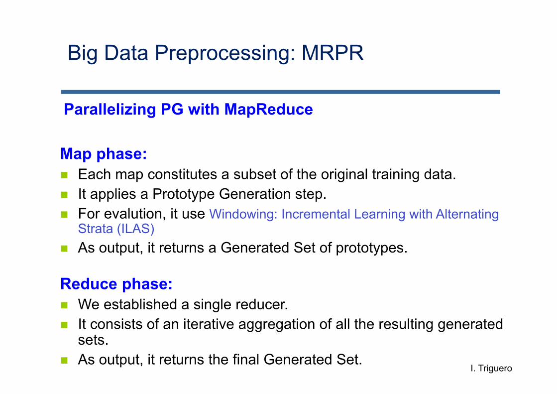
Parallelizing PG with MapReduce
Map phase: Each map constitutes a subset of the original training data. It applies a Prototype Generation step. For evalution, it use Windowing: Incremental Learning with Alternating
Strata (ILAS) As output, it returns a Generated Set of prototypes.
Reduce phase: We established a single reducer. It consists of an iterative aggregation of all the resulting generated
sets. As output, it returns the final Generated Set.
I. Triguero
Big Data Preprocessing: MRPR

The key of a MapReduce data partitioning approach is usually on the reduce phase.
Two alternative reducers: Join: Concatenates all the resulting generated sets.
This process does not guarantee that the final generated set does not contain irrelevant or even harmful instances
Fusion: This variant eliminates redundant prototypes by fusion of prototypes. Centroid-based PG methods: ICPL2 (Lam et al).
W. Lam et al, Discovering useful concept prototypes for classification based on filtering and abstraction. IEEE Transactions on Pattern Analysis and Machine Intelligence, vol. 14, no. 8, pp. 1075-1090, 2002
Parallelizing PG with MapReduce
I. Triguero
Big Data Preprocessing: MRPR

Windowing: Incremental Learning with Alternating Strata (ILAS)
J. Bacardit et al, Speeding-up pittsburgh learning classifier systems: Modeling time and accuracy In Parallel Problem Solving from Nature - PPSN VIII, ser. LNCS, vol. 3242, 2004, pp. 1021–1031
Training set is divided into strata, each iteration just uses one of the stratum.
Training set
0 Ex/n 2∙Ex/n Ex3∙Ex/n
Iterations
0 Iter
Main properties:Avoids a (potentially biased) static prototype selectionThis mechanism also introduces some generalization pressure
I. Triguero
Big Data Preprocessing: MRPR
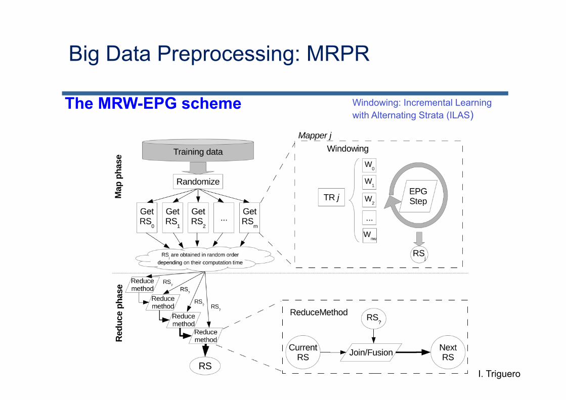
The MRW-EPG scheme Windowing: Incremental Learning with Alternating Strata (ILAS)
I. Triguero
Big Data Preprocessing: MRPR

Experimental Study
PokerHand data set. 1 million of instances, 3x5 fcv. Performance measures: Accuracy, reduction rate, runtime, test
classification time and speed up. PG technique tested: IPADECS.
I. Triguero
Big Data Preprocessing: MRPR

Results
PokerHand: Accuracy Test vs. Runtime results obtained by MRW-EPGI. Triguero
Big Data Preprocessing: MRPR

Results
I. Triguero
Big Data Preprocessing: MRPR

Results: Speed-up
I. Triguero
Big Data Preprocessing: MRPR

There is a good synergy between the windowing and MapReduce approaches. They complement themselves in the proposed two-level scheme.
Without windowing, evolutionary prototype generation could not be applied to data sets larger than approximately ten thousands instances
The application of this model has resulted in a very big reduction of storage requirements and classification time for the NN rule.
EPG for Big Data: Final Comments
I. Triguero
Big Data Preprocessing: MRPR

Complete study: I. Triguero, D. Peralta, J. Bacardit, S. García, F. Herrera. MRPR: A MapReduce solution for prototype reduction in big data classification. Neurocomputing 150 (2015) 331–345.
EPG for Big Data: Final Comments
Including: ENN algorithm for Filtering
Big Data Preprocessing: MRPR
https://github.com/triguero/MRPR

Fig. 6 Average runtime obtained by MRPR. (a) PokerHand
Complete study: I. Triguero, D. Peralta, J. Bacardit, S. García, F. Herrera. MRPR: A MapReduce solution for prototype reduction in big data classification. Neurocomputing 150 (2015) 331–345.
EPG for Big Data: Final Comments
Big Data Preprocessing: MRPR

• MRPG: A Combined MapReduce-Windowing Two-Level
Parallel Scheme for Evolutionary Prototype Generation
• MR-EFS: Evolutionary Feature Selection for Big Data
Classification: A MapReduce Approach
• Spark-ITFS: Filtering Feature Selection For Big Data
• Fast-mRMR: an optimal implementation of minimum
Redundancy Maximum Relevance algorithm
• Spark-MDLP: Distributed Entropy Minimization Discretizer for
Big Data Analysis under Apache Spark
Big Data Preprocessing
Describing some Approaches:
Big Data Preprocessing: MR-EFS
Evolutionary Feature Selection for Big Data Classification: A MapReduce Approach
D. Peralta, S. del Río, S. Ramírez-Gallego, I. Triguero, J.M. Benítez, F. Herrera. Evolutionary Feature Selection for Big Data Classification: A MapReduce Approach.Mathematical Problems in Engineering, 2015, In press.

Evolutionary Feature Selection (EFS)
Each individual represents a set of selected features (binary vector).
The individuals are crossed and mutated to generate new candidate sets of features.
Fitness function:Classification performance in the training dataset using only the features in the corresponding set.
Big Data Preprocessing: MR-EFS
D. Peralta

L. J. Eshelman, The CHC adaptative search algorithm: How to have safe search when engaging in nontraditional genetic recombination, in: G. J. E. Rawlins (Ed.), Foundations of Genetic Algorithms, 1991, pp. 265--283.
Evolutionary Algorithm: CHC
Big Data Preprocessing: MR-EFS
D. Peralta

Parallelizing FS with MapReduceMap phaseEach map task uses a subset of the training data.It applies an EFS algorithm (CHC) over the subset.A k-NN classifier is used for the evaluation of the population.Output (best individual):
Binary vector, indicating which features are selected.
Reduce phaseOne reducer.It sums the binary vectors obtained from all the map tasks.The output is a vector of integers.
Each element is a weight for the corresponding feature.
Big Data Preprocessing: MR-EFS
D. Peralta

MapReduce EFS process
Big Data Preprocessing: MR-EFS
The vector of weights is binarized with a threshold
D. Peralta

Dataset reduction
Big Data Preprocessing: MR-EFS
The maps remove the discarded features
No reduce phase
D. Peralta

Experimental Study: EFS scalability in MapReduce
0 5000 10000 15000 20000
050
000
1000
0015
0000
Number of instances
Tim
e (s
econ
ds)
Sequential CHCMR−EFSMR−EFS (full dataset)
CHC is quadratic w.r.t. the number of instances Splitting the dataset yields nearly quadratic acceleration
D. Peralta
Big Data Preprocessing: MR-EFS

Experimental Study: Classification
Two datasets epsilon ECBDL14, after applying
Random Oversampling
The reduction rate is controlled with the weight threshold
Three classifiers in Spark SVM Logistic Regression Naïve Bayes
Performance measures
Training runtime
D. Peralta
Big Data Preprocessing: MR-EFS

Experimental Study: results
0.64
0.66
0.68
0.70
500 1000 1500 2000Features
AU
C
Classifier
LogisticRegression
NaiveBayes
SVM−0.0
SVM−0.5
Set
Training
Test
D. Peralta
Big Data Preprocessing: MR-EFS

Experimental Study: Feature selection scalability
D. Peralta
Big Data Preprocessing: MR-EFS

The splitting of CHC provides several advantages: It enables tackling Big Data problems The speedup of the map phase is nearly quadratic The feature weight vector is more flexible than a binary vector
The data reduction process in MapReduce provides a scalable and flexible way to apply the feature selection
Both the accuracy and the runtime of the classification were improved after the preprocessing.
EFS for Big Data: Final Comments
D. Peralta
Big Data Preprocessing: MR-EFS
https://github.com/triguero/MR-EFS
• MRPG: A Combined MapReduce-Windowing Two-Level
Parallel Scheme for Evolutionary Prototype Generation
• MR-EFS: Evolutionary Feature Selection for Big Data
Classification: A MapReduce Approach
• Spark-ITFS: Filtering Feature Selection For Big Data
• Fast-mRMR: an optimal implementation of minimum
Redundancy Maximum Relevance algorithm
• Spark-MDLP: Distributed Entropy Minimization Discretizer for
Big Data Analysis under Apache Spark
Big Data Preprocessing
Describing some Approaches:

Filtering Feature Selection For Big Data
Many filtering methods are based on information theory. These are based on a quantitative criterion or index that measures its usefulness.
Relevance (self-interaction): mutual information of a feature with the class. Importance of a feature.
Redundancy (multi-interaction): conditional mutual information between two input features. Features that carry similar information.
S. Ramirez
Big Data Preprocessing: Spark-ITFS

Filtering Feature Selection For Big Data
There are a wide range of method in the literature built on these information theoretic measures.
To homogenize the use of all these criterions, Gavin Brown proposed a generic expression that allows to ensemble many of these criterions in an unique FS framework:
It is based on a greedy optimization which assesses features based on a simple scoring criterion. Through some independence assumptions, it allows to transform many criterions as linear combinations of Shannon entropy terms.
S. Ramirez
Brown G, Pocock A, Zhao MJ, Luján M (2012) Conditional likelihood max-imisation: A unifying framework for information theoretic feature selection. JMach Learn Res 13:27–66
Big Data Preprocessing: Spark-ITFS

Filtering Feature Selection For Big Data
S. Ramirez
Big Data Preprocessing: Spark-ITFS

Filtering Feature Selection For Big Data
We propose a distributed version of this framework based on a greedy approach (each iteration the algorithm selects one feature).
As relevance values do not change, we compute them first and cache to reuse.
Then, redundancy values are calculated between the non-selected features and the last one selected.
S. Ramirez
Big Data Preprocessing: Spark-ITFS

Filtering Feature Selection For Big Data
The most challengingpart is to compute the mutual and conditional information results.
It supposes to compute all combinations necessary for marginal and joint probabilities.
This imply to run several Map-Reduce phases to distribute and joint probabilities with its correspondent feature.
S. Ramirez
Big Data Preprocessing: Spark-ITFS

Filtering Feature Selection For Big Data
S. Ramirez
Group by type of probability(maintaining the origin)
(key, x, y, z, count) –Distinct by key Join by instance
Join by feature
Big Data Preprocessing: Spark-ITFS

Experimental Framework
Datasets: Two huge datasets (ECBDL14 and epsilon)
Parameters:
Measures: AUC, selection and classification time. Hardware: 16 nodes (12 cores per node), 64 GB RAM. Software: Hadoop 2.5 and Apache Spark 1.2.0.
S. Ramirez
Big Data Preprocessing: Spark-ITFS

Experimental Results: AUC and classification time
S. Ramirez
Big Data Preprocessing: Spark-ITFS

Experimental Results: Selection Time (in seconds)
S. Ramirez
Big Data Preprocessing: Spark-ITFS

Filtering Feature Selection For Big Data
Info-Theoretic Framework 2.0: Data column format: Row/Instance data are transformed to a column-wise
format. Each feature computation (X) is isolated and parallelized in each step. Cached marginal and joint probabilities: in order to reuse them in next
iterations. Broadcasted variables: Y and Z features and its marginal/joint values are
broadcasted in each iteration. Support for high-dimensional and sparse problems: zero values are
calculated from the non-zero values avoiding explosive complexity. Millions of features can be processed.
S. Ramirez
Code: http://spark-packages.org/package/sramirez/spark-infotheoretic-feature-selection
Big Data Preprocessing: Spark-ITFS

• MRPG: A Combined MapReduce-Windowing Two-Level
Parallel Scheme for Evolutionary Prototype Generation
• MR-EFS: Evolutionary Feature Selection for Big Data
Classification: A MapReduce Approach
• Spark-ITFS: Filtering Feature Selection For Big Data
• Fast-mRMR: an optimal implementation of minimum
Redundancy Maximum Relevance algorithm
• Spark-MDLP: Distributed Entropy Minimization Discretizer for
Big Data Analysis under Apache Spark
Big Data Preprocessing
Describing some Approaches:

Fast-mRMR: an optimal implementation of minimum Redundancy Maximum Relevance algorithmOriginal proposal (mRMR): Rank features based on their relevance to the target, and at the same
time, the redundancy of features is also penalized. Maximum dependency: mutual information (MI) between a feature set
S with xi features and the targe class c:
Minimum redundancy: MI between features.
Combining two criterions:
S. Ramirez
Hanchuan Peng, Fulmi Long, and Chris Ding. Feature selection based on mutual information criteria of max-dependency, max-relevance, and min-redundancy. Pattern Analysis and Machine Intelligence, IEEE Transactions on, 27(8):1226–1238, 2005.
Big Data Preprocessing: Fast-mRMR

Fast-mRMR: an optimal implementation of minimum Redundancy Maximum Relevance algorithmImprovements:
Accumulating Redundancy (greedy approach): in each iteration only compute MI between last selected feature and those non-selected. Select one feature by iteration.
Data-access pattern: column-wise format (more natural approach). Caching marginal probabilities: computed once at the beginning,
saving extra computations.
S. Ramirez
Big Data Preprocessing: Fast-mRMR

Fast-mRMR: an optimal implementation of minimum Redundancy Maximum Relevance algorithmSoftware package with several versions for:
CPU: implemented in C++. For small and medium datasets. GPU: mapped MI computation problem to histogramming problem in
GPU. Parallel version. Apache Spark: for Big Data problems.
S. Ramirez
Code: https://github.com/sramirez/fast-mRMR
Big Data Preprocessing: Fast-mRMR

Fast-mRMR: an optimal implementation of minimum Redundancy Maximum Relevance algorithm
S. Ramirez
Big Data Preprocessing: Fast-mRMR

• MRPG: A Combined MapReduce-Windowing Two-Level
Parallel Scheme for Evolutionary Prototype Generation
• MR-EFS: Evolutionary Feature Selection for Big Data
Classification: A MapReduce Approach
• Spark-ITFS: Filtering Feature Selection For Big Data
• Fast-mRMR: an optimal implementation of minimum
Redundancy Maximum Relevance algorithm• Spark-MDLP: Distributed Entropy Minimization Discretizer for
Big Data Analysis under Apache Spark
Big Data Preprocessing
Describing some Approaches:

Distributed Entropy Minimization Discretizer forBig Data Analysis under Apache Spark
Sergio Ramírez-Gallego, Salvador García, Héctor Mouriño-Talín, David Martínez-Rego ,Verónica Bolón-Canedo, Amparo Alonso-Betanzos, José Manuel Benítez, Francisco Herrera Distributed Entropy Minimization Discretizer for Big Data Analysis under Apache Spark.IEEE BigDataSE, 2015.
I. Triguero
Big Data Preprocessing: Spark-MDLP

Introduction
The astonishing rate of data generation on the Internet nowadays has caused that many classical knowledge extraction techniques have become obsolete.
Data reduction (discretization) techniques are required in order to reduce the complexity order held by these techniques.
In spite of the great interest, only a few simple discretization techniques have been implemented in the literature for Big Data.
We propose a distributed implementation of the entropy minimization discretizer proposed by Fayyad and Irani using Apache Spark platform.
S. Ramirez
U. M. Fayyad and K. B. Irani, “Multi-interval discretization of continuous-valued attributes for classification learning,” in International Joint Conference On Artificial Intelligence, vol. 13. Morgan Kaufmann, 1993, pp. 1022–1029.
Resilient Distributed Datasets: A Fault-Tolerant Abstraction for In-Memory Cluster Computing. Matei Zaharia, Mosharaf Chowdhury, Tathagata Das, Ankur Dave, Justin Ma, Murphy McCauley, Michael J. Franklin, Scott Shenker, Ion Stoica. NSDI 2012. April 2012.
Big Data Preprocessing: Spark-MDLP

Discretization: An Entropy Minimization Approach
Discretization: transforms numerical attributes into discrete or nominal attributes with a finite number of intervals.
Main objective: find the best set of points/intervals according to a quality measure (e.g.: inconsistency or entropy).
Optimal discretization is NP-complete, determined by the number of candidate cut points (all distinct values in the dataset for each attribute).
A possible optimization: use only boundary points in the whole set (midpoint between two values between two classes).
S. Ramirez
U. M. Fayyad and K. B. Irani, “Multi-interval discretization of continuous-valued attributes for classification learning,” in International Joint Conference On Artificial Intelligence, vol. 13. Morgan Kaufmann, 1993, pp. 1022–1029.
S. García, J. Luengo, and F. Herrera, Data Preprocessing in DataMining. Springer, 2015.
Big Data Preprocessing: Spark-MDLP

Discretization: An Entropy Minimization Approach
Minimum Description Length Discretizer (MDLP) implements this optimization and multi-interval extraction of points (which improves accuracy and simplicity respect to ID-3).
Quality measure: class entropy of partitioning schemes (S1, S2) for attribute A. Find the best cut point.
Stop criterion: MDLP criterion
S. Ramirez
U. M. Fayyad and K. B. Irani, “Multi-interval discretization of continuous-valued attributes for classification learning,” in International Joint Conference On Artificial Intelligence, vol. 13. Morgan Kaufmann, 1993, pp. 1022–1029.
Big Data Preprocessing: Spark-MDLP

Distributed MDLP Discretization: a complexity study
Determined by two time-consuming operations (repeated for each attribute):– Sorting: O(|A| log |A|), assuming A is an attribute with all its points
distinct.– Evaluation: quadratic operation (boundary points).
Proposal:– Sort all points in the dataset using a single distributed operation.– Evaluates boundary points (per feature) in an parallel way.
Main Primitives: using Apache Spark, a large-scale processing framework based on in-memory primitives. Some primitives used:– SortByKey: sort tuples by key in each partition. Partitions are also
sorted.– MapPartitions: an extension of Map-Reduce operation for partition
processing.S. Ramirez
Big Data Preprocessing: Spark-MDLP

Distributed MDLP Discretization: main procedure
1) Distinct points: it creates tupleswhere key is formed by the feature index and the value. Value: frequency vector for classes.
2) Sorting: distinct points are sorted by key (feature, value).
3) Boundary points: boundary points are calculated evaluating consecutives points.
4) Points grouped by feature: grouped and new key: only the attribute index.
5) Attributes divided by size: depends on the number of boundary points (> 10,000 points)
6) Points selection and MLDP evaluation
S. Ramirez
Big Data Preprocessing: Spark-MDLP

Distributed MDLP Discretization: main procedure1) Distinct points: already
calculated in step #1 from raw data.
2) Sorting: distinct points are sorted by key. For the next step, the first points in each partition are sent to the following partition.
3) Boundary points: midpoints are generated when two points of the same attribute are on the border. Last points in a partition and in a feature are also added.
4) MLDP selection and evaluation: parallelized by feature
S. Ramirez
Big Data Preprocessing: Spark-MDLP

Distributed MDLP Discretization: attribute division
Once boundary points are generated, for each attribute do: Points < limit: group in a
local list. Point > limit: associate a
list of partitions (distributed) → unusual.
Then, the points are evaluated recursively,depending of the aforementiond parameter. In case of partitions, the process is iterative, whereas for list of points, it is distributed.
S. Ramirez
Big Data Preprocessing: Spark-MDLP

Distributed MDLP Discretization: MDLP evaluation (small)
1)Prerequisites: Points must be sorted.
2)Compute the total frequency for all classes
3)For each point: Left accumulator:
computed from the left. Right accumulator:
computed using the left one and the total,
4) The point is evaluated as:
(point, frequency, left, right)
S. Ramirez
Big Data Preprocessing: Spark-MDLP

Distributed MDLP Discretization: MDLP evaluation (big)
1)Prerequisites: Points and partitions must be sorted
2)Compute the total frequency by partition
3) Compute the accumulated frequency
4)For each partition: Left accumulator:
computed from the left. Right accumulator:
computed using the left one and the total,
5) The point is evaluated as: (point, frequency, left, right).
S. Ramirez
Big Data Preprocessing: Spark-MDLP

Experimental Framework
Datasets: Two huge datasets (ECBDL14 and epsilon)
Parameters: 50 intervals and 100,000 max candidates per partition. Classifier: Naive Bayes from MLLib, lambda = 1, iterations = 100. Measures: discretization time, classification time and classification accuracy. Hardware: 16 nodes (12 cores per node), 64 GB RAM. Software: Hadoop 2.5 and Apache Spark 1.2.0.
S. Ramirez
Big Data Preprocessing: Spark-MDLP

Performance results: Classification accuracy
Clear advantage on using discretization in both datasets. Specially important for ECBDL14.
S. Ramirez
Big Data Preprocessing: Spark-MDLP

Performance results: Classification time modelling
Light improvement between both versions. It seems that using discretization does not affect too much the modelling performance.
Despite of being insignificant, the time value for discretization is a bit better than for the other one.
S. Ramirez
Big Data Preprocessing: Spark-MDLP

Performance results: Discretization time
High speedup between the sequential version and the distributed one for both datasets.
For ECBDL14, our version is almost 300 times faster. Even for the medium-size dataset (epsilon), there is a clear advantage.
The bigger the dataset, the higher the improvement.
S. Ramirez
Big Data Preprocessing: Spark-MDLP

Spark-MDLP: Final Comments
We have proposed a sound multi-interval discretization methodbased on entropy minimization for large-scale discretization. This has implied a complete redesign of the original proposal.
Adapting discretization methods to Big Data is not a trivial task (only few simple techniques implemented).
The experimental results has demonstrated the improvement in accuracy and time (both classification and discretization) with respect to the sequential proposal.
S. Ramirez
Big Data Preprocessing: Spark-MDLP
https://github.com/sramirez/spark-MDLP-discretization

216
Outline
Big Data. Big Data Science. Data Preprocessing
Why Big Data? MapReduce Paradigm. Hadoop Ecosystem
Big Data Classification: Learning algorithms
Data Preprocessing
Big data Preprocessing
Imbalanced Big Data Classification: Data preprocessing
Challenges and Final Comments

Objective: Contact map prediction
Details: 32 million instances 631 attributes (539 real & 92 nominal values) 2 classes 98% of negative examples About 56.7GB of disk space
Evaluation:True positive rate · True negative rate TPR · TNR
J. Bacardit et al, Contact map prediction using a large-scale ensemble of rule sets and the fusion of multiplepredicted structural features, Bioinformatics 28 (19) (2012) 2441-2448
http://cruncher.ncl.ac.uk/bdcomp/index.pl?action=data
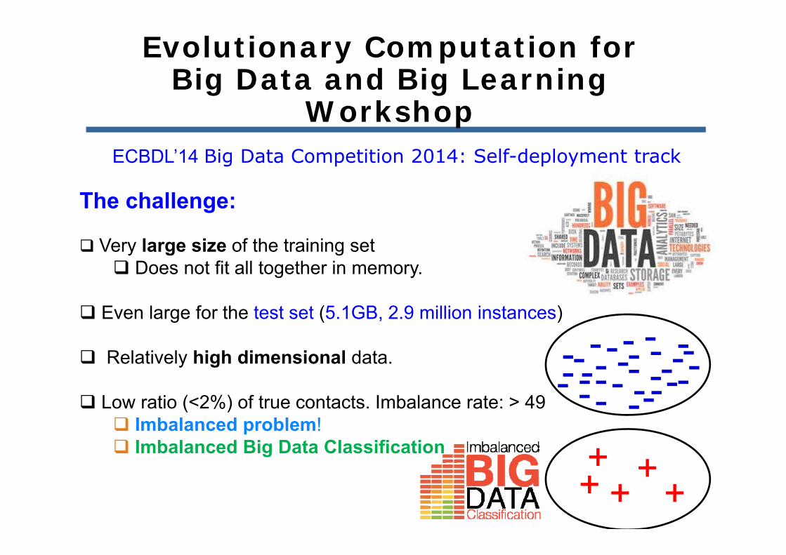
ECBDL’14 Big Data Competition 2014: Self-deployment track
Evolutionary Computation for Big Data and Big Learning
Workshop
Evolutionary Computation for Big Data and Big Learning
WorkshopECBDL’14 Big Data Competition 2014: Self-deployment track
The challenge:
Very large size of the training set Does not fit all together in memory.
Even large for the test set (5.1GB, 2.9 million instances)
Relatively high dimensional data.
Low ratio (<2%) of true contacts. Imbalance rate: > 49 Imbalanced problem! Imbalanced Big Data Classification
--
-- ----
- --
------
-- -- -- -
- ---- - -
++ +++

We need tochange the wayto evaluate a modelperformance!
Imbalanced classes problem: standard learners are often biased towards the majority class.
Imbalanced Big Data ClassificationIntroduction

Imbalanced Big Data ClassificationIntroduction
Over-SamplingRandomFocused
Under-SamplingRandomFocused
Cost Modifying (cost-sensitive)
Motivation
Retain influential examplesBalance the training set
Remove noisy instances in the decision boundariesReduce the training set
Strategies to deal with imbalanced data sets
Algorithm-level approaches: A commont strategy to deal with the class imbalance is to choose an appropriate inductive bias.Boosting approaches: ensemble learning, AdaBoost, …

A MapReduce Approach
Over-SamplingRandomFocused
Under-SamplingRandomFocused
Cost Modifying (cost-sensitive)Boosting/Bagging approaches (withpreprocessing)
Previous study on extremely imbalanced big data: S. Río, V. López, J.M. Benítez, F. Herrera, On the use of MapReduce for Imbalanced Big Data using Random Forest. Information Sciences 285 (2014) 112-137.
Imbalanced Big Data Classification
32 million instances, 98% of negative examples. Low ratio of true contacts (<2%). Imbalance rate: > 49. Imbalanced problem!

S. Río, V. López, J.M. Benítez, F. Herrera, On the use of MapReduce for Imbalanced Big Data using Random Forest. Information Sciences 285 (2014) 112-137.
A MapReduce Approach for Random Undersampling
Imbalanced Big Data Classification

S. Río, V. López, J.M. Benítez, F. Herrera, On the use of MapReduce for Imbalanced Big Data using Random Forest. Information Sciences 285 (2014) 112-137.
A MapReduce Approach for Random Oversampling
Imbalanced Big Data Classification

S. Río, V. López, J.M. Benítez, F. Herrera, On the use of MapReduce for Imbalanced Big Data using Random Forest. Information Sciences 285 (2014) 112-137.
A MapReduce Approach for Adapting the generation of synthetic minority samples
Imbalanced Big Data Classification

Analysis of the effectiveness in classification of the approaches
Potential problem: lack of density of the positive class for RUS/SMOTE. Lack of data due to the data fragmentation for MapReduce
Imbalanced Big Data Classification
https://github.com/saradelrio/hadoop-imbalanced-preprocessing
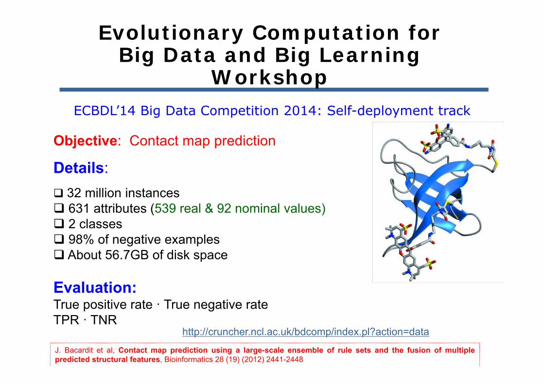
Objective: Contact map prediction
Details: 32 million instances 631 attributes (539 real & 92 nominal values) 2 classes 98% of negative examples About 56.7GB of disk space
Evaluation:True positive rate · True negative rate TPR · TNR
J. Bacardit et al, Contact map prediction using a large-scale ensemble of rule sets and the fusion of multiplepredicted structural features, Bioinformatics 28 (19) (2012) 2441-2448
http://cruncher.ncl.ac.uk/bdcomp/index.pl?action=data
ECBDL’14 Big Data Competition 2014: Self-deployment track
Evolutionary Computation for Big Data and Big Learning
Workshop

ECBDL’14 Big Data Competition 2014
Our approach:
1. Balance the original training data Random Oversampling (As first idea, it was extended)
2. Learning a model. Random Forest
ECBDL’14 Big Data Competition

ECBDL’14 Big Data Competition

We initially focused on
Oversampling rate: {100%}
RandomForest: Number of used features: 10 (log n +1); Number of trees: 100 Number of maps: {64, 190, 1024, 2048}
To higher mappers, the lowest TPR (relevant!)
Nº mappers TPR_tst TNR_tstTNR*TPR
Test64 0,601723 0,806269 0,485151190 0,635175 0,773308 0,4911861024 0,627896 0,756297 0,4748762048 0,624648 0,759753 0,474578
ECBDL’14 Big Data Competition

ECBDL’14 Big Data Competition
Oversampling rate: {100%}RandomForest

ECBDL’14 Big Data Competition

We initially focused on
Oversampling rate: 100%RandomForest: Number of used features: 10 (log n +1); Number of trees: 100 Number of maps: {64, 190, 1024, 2048}
Very low TPR (relevant!)
Nº mappers TPR_tst TNR_tstTNR*TPR
Test190 0,635175 0,773308 0,491186
How to increase the TPR rate?
Idea: To increase the ROS percentaje
ECBDL’14 Big Data Competition

How to increase the TPR rate? Idea: To increase the ROS percentaje
Oversampling rate: {100, 105, 110, 115, 130}
RandomForest: Number of used features:10; Number of trees: 100
The higher ROS percentage, the higher TPR and the lower TNR
Algorithms TPR TNRTNR*TPR
TestROS+RF (RS: 100%) 0.6351 0.7733 0.491186ROS+RF (RS: 105%) 0.6568 0.7555 0.496286ROS+RF (RS: 110%) 0.6759 0.7337 0.495941ROS+RF (RS: 115%) 0.7041 0.7103 0.500175ROS+RF (RS: 130%) 0.7472 0.6609 0.493913
ECBDL’14 Big Data Competition

ECBDL’14 Big Data Competition

ECBDL’14 Big Data Competition
What can we do?

ECBDL’14 Big Data Competition 2014
Our approach:
1. Balance the original training data Random Oversampling (As first idea, it was extended)
2. Learning a model. Random Forest
3. Detect relevant features. Evolutionary Feature Selection
Classifying test set.
ECBDL’14 Big Data Competition

ECBDL’14 Big Data Competition
Feature selection does not help us

ECBDL’14 Big Data Competition 2014
Our approach:
1. Balance the original training data Random Oversampling (As first idea, it was extended)
2. Learning a model. Random Forest
3. Detect relevant features. Evolutionary Feature Weighting
Classifying test set.
ECBDL’14 Big Data Competition

Third component: MapReduce Approach for Feature Weightingfor getting a major performance over classes
Map Side Each map read one block from dataset. Perform an Evolutionary Feature Weighting step. Output: a real vector that represents the degree of importance of each feature.Number of maps: 32768 (less than 1000 original data per map)
Reduce Side Aggregate the feature’s weights A feature is finally selected if it overcomes a given threshold. Output: a binary vector that represents the final selection
I. Triguero, J. Derrac, S. García, F. Herrera, Integrating a Differential Evolution Feature Weighting scheme into PrototypeGeneration. Neurocomputing 97 (2012) 332-343
ECBDL’14 Big Data Competition
How to increase the performance?

Third component: MapReduce Approach for Feature Weightingfor getting a major performance over classes
ECBDL’14 Big Data Competition
How to increase the performance?

Random Oversampling: Oversampling ratio. Analyzed values: {100 to 130)
Feature Weigthing:
Threshold --> number of selected features. Set of features: {19, 63, 90, 146} Number of maps: 32768
RandomForest:
Number of used features: {log NumFeatures, 2 * Log +1} Number of trees: {100} Number of maps: {32, 64,128, 190, 256, 512}
Experimental study
ECBDL’14 Big Data Competition
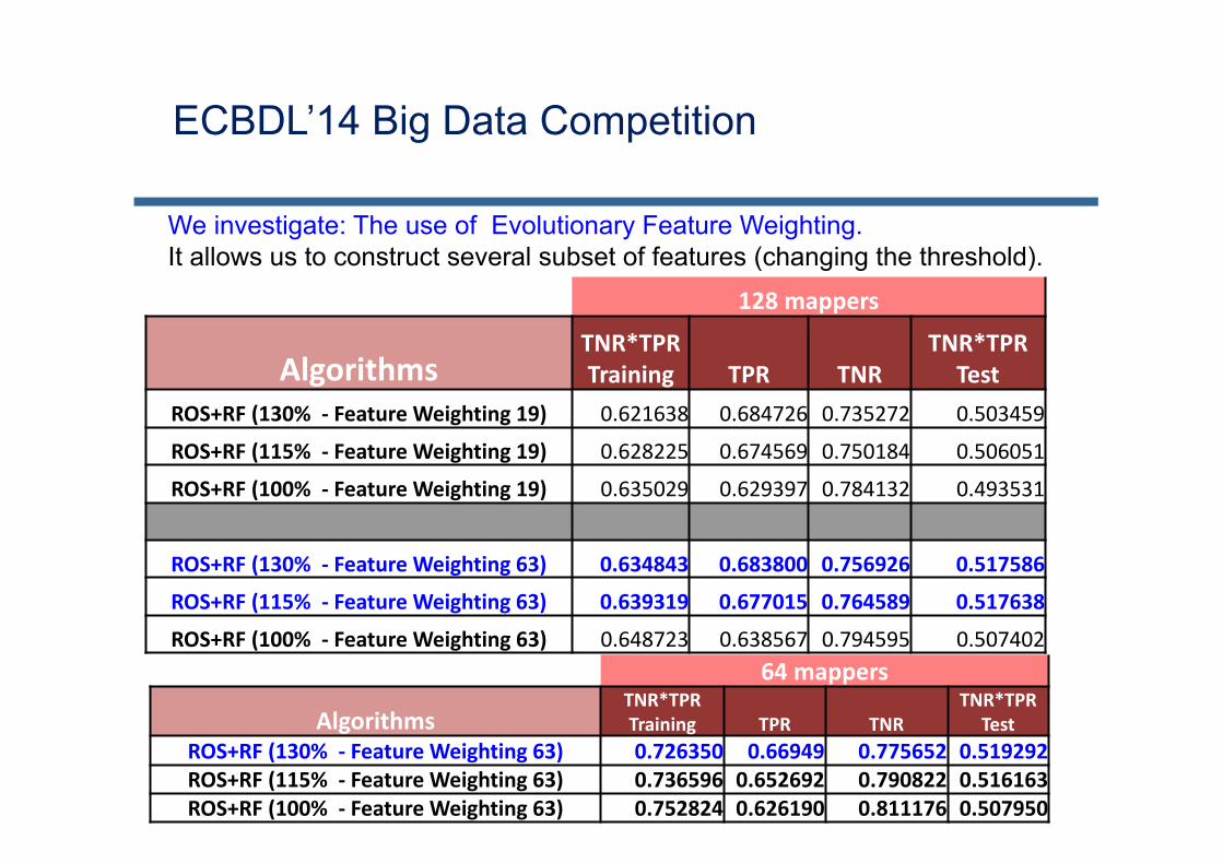
We investigate: The use of Evolutionary Feature Weighting. It allows us to construct several subset of features (changing the threshold).
128 mappers
AlgorithmsTNR*TPR Training TPR TNR
TNR*TPRTest
ROS+RF (130% ‐ Feature Weighting 19) 0.621638 0.684726 0.735272 0.503459
ROS+RF (115% ‐ Feature Weighting 19) 0.628225 0.674569 0.750184 0.506051
ROS+RF (100% ‐ Feature Weighting 19) 0.635029 0.629397 0.784132 0.493531
ROS+RF (130% ‐ Feature Weighting 63) 0.634843 0.683800 0.756926 0.517586
ROS+RF (115% ‐ Feature Weighting 63) 0.639319 0.677015 0.764589 0.517638
ROS+RF (100% ‐ Feature Weighting 63) 0.648723 0.638567 0.794595 0.50740264 mappers
AlgorithmsTNR*TPR Training TPR TNR
TNR*TPR Test
ROS+RF (130% ‐ Feature Weighting 63) 0.726350 0.66949 0.775652 0.519292ROS+RF (115% ‐ Feature Weighting 63) 0.736596 0.652692 0.790822 0.516163ROS+RF (100% ‐ Feature Weighting 63) 0.752824 0.626190 0.811176 0.507950
ECBDL’14 Big Data Competition

Evolutionary Feature Weighting. It allows us to construct several subset of features (changing the threshold).
64 mappers
AlgorithmsTNR*TPR Training TPR TNR
TNR*TPR Test
ROS+RF (130% ‐ Feature Weighting 63) 0.726350 0.66949 0.775652 0.519292ROS+RF (115% ‐ Feature Weighting 63) 0.736596 0.652692 0.790822 0.516163ROS+RF (100% ‐ Feature Weighting 63) 0.752824 0.626190 0.811176 0.507950
ECBDL’14 Big Data Competition

ECBDL’14 Big Data Competition
ROS (130) + Evolutionary Feature Weighting

64 mappers
AlgorithmsTNR*TPRTraining TPR TNR
TNR*TPRTest
ROS+ RF (130%+ FW 90+25f+200t) 0.736987 0.671279 0.783911 0.526223ROS+ RF (140%+ FW 90+25f+200t) 0.717048 0.695109 0.763951 0.531029
190 mappers
AlgorithmsTNR*TPRTraining TPR TNR
TNR*TPR Test
ROS+ RF (140%+ FW 90+25f+200t) 0.629273 0.721652 0.729740 0.526618
64 mappers and we got 0.53
ROS 130 – 65 replications of the minority instances (ROS 140 – 68)
More features with diffferent Maps configuration
ECBDL’14 Big Data Competition

ECBDL’14 Big Data Competition

Current state:
Our knowledge: The higher ROS percentage, the higher TPR and the lower TNR
The less number of maps, the less TPR and the high TNR (highaccuracy).
4 days to finish the competion:
Can we take decisions to improve the model?
64 mappers
AlgorithmsTNR*TPRTraining TPR TNR
TNR*TPRTest
ROS+ RF (140%+ FW 90+25f+200t) 0.717048 0.695109 0.763951 0.531029
ECBDL’14 Big Data Competition
ROS 130 – 65 (140 – 68) replications of the minority instances

64 mappers
AlgorithmsTNR*TPRTraining TPR TNR
TNR*TPRTest
ROS+ RF (130%+ FW 90+25f+200t) 0.736987 0.671279 0.783911 0.526223ROS+ RF (140%+ FW 90+25f+200t) 0.717048 0.695109 0.763951 0.531029ROS+ RF (150%+ FW 90+25f+200t) 0.706934 0.705882 0.753625 0.531971ROS+ RF (160%+ FW 90+25f+200t) 0,698769 0.718692 0.741976 0.533252ROS+ RF (170%+ FW 90+25f+200t) 0.682910 0.730432 0.730183 0.533349ROS+ RF (180%+ FW 90+25f+200t) 0,678986 0.737381 0.722583 0.532819
Last decision: We investigated to increase ROS until 180% with 64 mappers
To increase ROS and reduce the mappers number lead us to get a trade-off with good results
ROS 170 – 85 replications of the minority instances
ECBDL’14 Big Data Competition
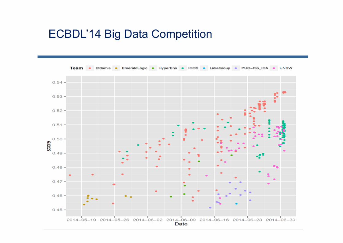
ECBDL’14 Big Data Competition

Results of the competition: Contact map prediction
Team Name TPR TNR Acc TPR · TNREfdamis 0.730432 0.730183 0.730188 0.533349ICOS 0.703210 0.730155 0.729703 0.513452UNSW 0.699159 0.727631 0.727153 0.508730HyperEns 0.640027 0.763378 0.761308 0.488583
PUC-Rio_ICA 0.657092 0.714599 0.713634 0.469558Test2 0.632009 0.735545 0.733808 0.464871EmeraldLogic 0.686926 0.669737 0.670025 0.460059
LidiaGroup 0.653042 0.695753 0.695036 0.454356
http://cruncher.ncl.ac.uk/bdcomp/index.pl?action=ranking
Evolutionary Computation for Big Data and Big Learning Workshop
EFDAMIS team ranked first in the ECBDL’14 big data competition
ECBDL’14 Big Data Competition

ECBDL’14 Big Data Competition

At the beginning ROS+RF (RS: 100%)
Nº mappers TPR_tst TNR_tstTNR*TPR
Test64 0,601723 0,806269 0,485151
At the end: ROSEFW-RF algorithm
64 mappers
AlgorithmsTNR*TPRTraining TPR TNR
TNR*TPRTest
ROS+ RF (160%+ FW 90+25f+200t) 0,698769 0.718692 0.741976 0.533252ROS+ RF (170%+ FW 90+25f+200t) 0.682910 0.730432 0.730183 0.533349ROS+ RF (180%+ FW 90+25f+200t) 0,678986 0.737381 0.722583 0.532819
ECBDL’14 Big Data CompetitionFinal comments
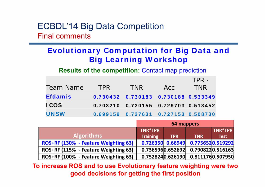
Results of the competition: Contact map prediction
Team Name TPR TNR AccTPR · TNR
Efdamis 0.730432 0.730183 0.730188 0.533349ICOS 0.703210 0.730155 0.729703 0.513452UNSW 0.699159 0.727631 0.727153 0.508730
To increase ROS and to use Evolutionary feature weighting were two good decisions for getting the first position
Evolutionary Computation for Big Data and Big Learning Workshop
64 mappers
AlgorithmsTNR*TPR Training TPR TNR
TNR*TPR Test
ROS+RF (130% ‐ Feature Weighting 63) 0.726350 0.66949 0.7756520.519292ROS+RF (115% ‐ Feature Weighting 63) 0.7365960.652692 0.7908220.516163ROS+RF (100% ‐ Feature Weighting 63) 0.7528240.626190 0.8111760.507950
ECBDL’14 Big Data CompetitionFinal comments

ECBDL’14 Big Data CompetitionFinal comments
Experiments with 64 mapsROS 170 – 85 replications of the minority instancesRemember the initial problem. Lack of density of the minority class
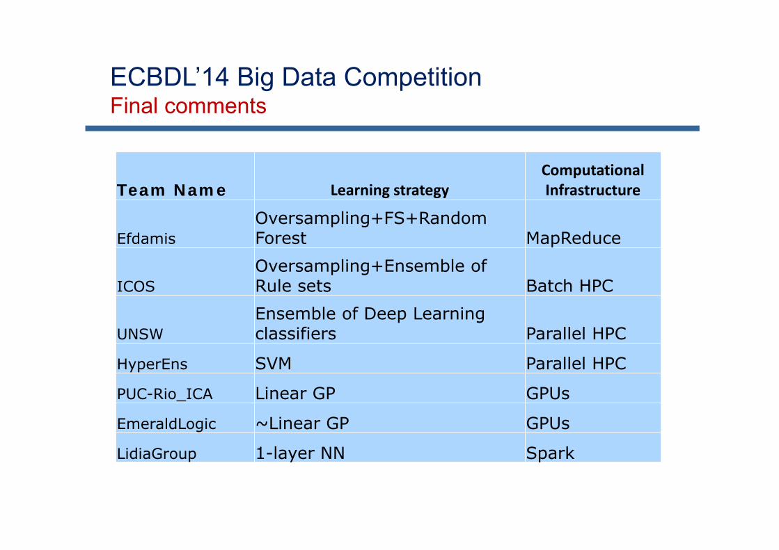
ECBDL’14 Big Data CompetitionFinal comments
Team Name Learning strategyComputationalInfrastructure
EfdamisOversampling+FS+RandomForest MapReduce
ICOS Oversampling+Ensemble of Rule sets Batch HPC
UNSW Ensemble of Deep Learning classifiers Parallel HPC
HyperEns SVM Parallel HPC
PUC-Rio_ICA Linear GP GPUs
EmeraldLogic ~Linear GP GPUs
LidiaGroup 1-layer NN Spark

ECBDL’14 Big Data CompetitionOur algorithm: ROSEFW-RF
I. Triguero, S. del Río, V. López, J. Bacardit, J.M. Benítez, F. Herrera. ROSEFW-RF: The winner algorithm for the ECBDL'14 Big Data Competition: An extremely imbalanced big data bioinformatics problem. Knowledge-Based Systems, 2015, In press.
https://github.com/triguero/ROSEFW-RF

257
Outline
Big Data. Big Data Science. Data Preprocessing
Why Big Data? MapReduce Paradigm. Hadoop Ecosystem
Big Data Classification: Learning algorithms
Data Preprocessing
Big data Preprocessing
Big Data Classification: Imbalanced classes and data preprocessing
Challenges and Final Comments

Final Comments
Data Mining, Machine learning and data preprocessing: Huge collection of algorithms
Big Data: A small subset of algorithms
Big Data Preprocessing: A few methods for preprocessing in Big Data analytics.

Some Challenges on Big Data Preprocessing
Big Data Reduction To improve the efficiency in
the big data analytics. Quality data for quality
models in big data analytics
Final Comments
Clean Big Data Noise in data distorts
Computation results Search results
Need automatic methods for “cleaning” the data Duplicate elimination Quality evaluation
Missing values Missing values management
Computing Model Accuracy and Approximation Efficiency

Final Remarks
Big Data Preprocessing
Big data preprocessing methods are necessary to improve the quality of the processes of big
data analytics.
Quality decisions must be based on quality big data!

Final Comments

Data Mining methods for Big Data Preprocessing


![Data Mining - [1] Data - 03 - Preprocessing...Data Mining –Fabio Stella Data: EXPLORATION Transcription and interpretation errors are responsibility of the lecturer. Pang-Ning Tan,](https://static.fdocuments.us/doc/165x107/612995dcb03af37b5d636341/data-mining-1-data-03-preprocessing-data-mining-afabio-stella-data.jpg)