Karsten Borgwardt: Data Mining in Bioinformatics, Page 1

Data Mining in BioinformaticsDay 1: Classification

Karsten Borgwardt

February 18 to March 1, 2013

Machine Learning & Computational Biology Research GroupMax Planck Institute Tübingen and

Eberhard Karls Universität Tübingen

Our course

Karsten Borgwardt: Data Mining in Bioinformatics, Page 2

ScheduleFebruary 18 to March 1Lecture from 10:00 to 12:30, tutorials are projected-basedOral exam on March 5 to get the certificate

Structure1 week of algorithmics, 1 week of bioinformatics appli-cationsKey topics: classification, clustering, feature selection,text & graph miningLecture will provide introduction to the topic + discussionof important papers

What is data mining?

Karsten Borgwardt: Data Mining in Bioinformatics, Page 3

Data MiningExtracting knowledge from large amounts of data (Hanand Kamber, 2006)Often used as synonym for Knowledge Discovery — yetother definitions disagree

Knowledge DiscoveryData cleaningData integrationData selectionData transformationData miningPattern evaluationKnowledge presentation

What is classification?

Karsten Borgwardt: Data Mining in Bioinformatics, Page 4

ProblemGiven an object, which class of objects does it belongto?Given object x, predict its class label y.

ExamplesComputer vision: Is this object a chair?Credit cards: Is this customer to be trusted?Marketing: Will this customer buy/like our product?Function prediction: Is this protein an enzyme?Gene finding: Does this sequence contain a splice site?

What is classification?

Karsten Borgwardt: Data Mining in Bioinformatics, Page 5

SettingClassification is usually performed in a supervised set-ting: We are given a training dataset.A training dataset is a dataset of pairs (xi, yi), that isobjects and their known class labelsThe test set is a dataset of test points x′ with unknownclass labelThe task is to predict the class label y′ of x′

Role of yif y ∈ {0, 1}: then we are dealing with a binary classi-fication problemif y ∈ {1, . . . , n}, (n ∈ N): a multiclass classificationproblemif y ∈ R: a regression problem

Classifiers in a nutshell

Karsten Borgwardt: Data Mining in Bioinformatics, Page 6

Nearest NeighbourKey idea: if x1 is most similar to x2, then y1 = y2Classification by looking at the ‘Nearest Neighbour’

Naive BayesA simple probabilistic classifier based on applyingBayes’ theorem with strong (naive) independence as-sumptions

Decision treesA series of decisions has to be taken to classify an ob-ject, based on its attributesThe hierarchy of these decisions is ordered as a tree, a‘decision tree’.

Classifiers in a nutshell

Karsten Borgwardt: Data Mining in Bioinformatics, Page 7

Support Vector MachineKey idea: Draw a line (plane, hyperplane) that separatestwo classes of dataMaximise the distance between the hyperplane and thepoints closest to it (margin)Test point is predicted to belong to the class whose half-space it is located in

Criteria for a good classifierAccuracyRuntime and scalabilityInterpretabilityFlexibility

Nearest Neighbour

Karsten Borgwardt: Data Mining in Bioinformatics, Page 8

The actual classificationGiven xi, we predict its label yi by

xj = argminx∈D||x− xi||2 ⇒ yi = yj (1)

xi’s predicted label is that of the point closest to it, thatis its ‘nearest neighbour’

RuntimeNaively, one has to compute the distance to all N neigh-bours in the dataset for each point:O(N) for one pointO(N 2) for the entire dataset

Nearest Neighbour

Karsten Borgwardt: Data Mining in Bioinformatics, Page 9

How to speed NN upExploit the triangle inequality:

d(x1, x2) + d(x2, x3) ≥ d(x1, x3) (2)

This holds for any metric d.

MetricA distance function d is a metric iff1. d(x1, x2) ≥ 02. d(x1, x2) = 0 if and only if x1 = x23. d(x1, x2) = d(x2, x1)4. d(x1, x3) ≤ d(x1, x2) + d(x2, x3)

Nearest Neighbour

Karsten Borgwardt: Data Mining in Bioinformatics, Page 10

How to speed NN upRewrite triangle inequality:

d(x1, x2) ≥ d(x1, x3)− d(x2, x3) (3)

That means if you know d(x1, x3) and d(x2, x3), you canprovide a lower bound on d(x1, x2)

If you know a point that is closer to x1 than d(x1, x3) −d(x2, x3), then you can avoid to compute d(x1, x2)

Naive Bayes

Karsten Borgwardt: Data Mining in Bioinformatics, Page 11

Bayes’ Rule

P (C|x) =P (x|C)P (C)

P (x)(4)

Naive Bayes ClassificationClassify x into one of m classes C1, . . . , Cm

argmaxCiP (Ci|x) =

P (x|Ci)P (Ci)

P (x)(5)

Naive Bayes

Karsten Borgwardt: Data Mining in Bioinformatics, Page 12

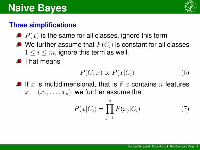
Three simplificationsP (x) is the same for all classes, ignore this termWe further assume that P (Ci) is constant for all classes1 ≤ i ≤ m, ignore this term as well.That means

P (Ci|x) ∝ P (x|Ci) (6)

If x is multidimensional, that is if x contains n featuresx = (x1, . . . , xn), we further assume that

P (x|Ci) =n∏j=1

P (xj|Ci) (7)

Naive Bayes

Karsten Borgwardt: Data Mining in Bioinformatics, Page 13

The actual classificationThe actual classification is performed by computing

P (Ci|x) ∝n∏j=1

P (xj|Ci) (8)

The three simplifications are thatall classes have the same marginal probabilityall data points have the same marginal probabilityall features of an object are independent of each other

Alternative name:‘Simple Bayes Classifier’

RuntimeO(Nmn), where N is the number of data points, m thenumber of classes, n the number of features

Decision Tree

Karsten Borgwardt: Data Mining in Bioinformatics, Page 14

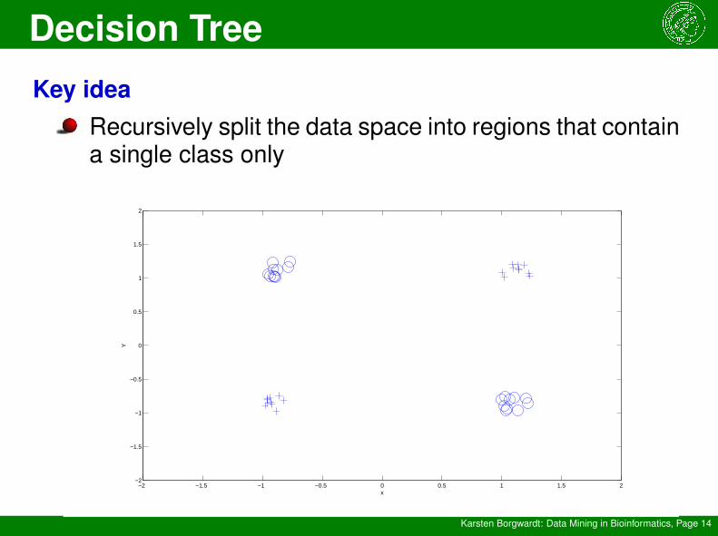
Key ideaRecursively split the data space into regions that containa single class only

−2 −1.5 −1 −0.5 0 0.5 1 1.5 2−2

−1.5

−1

−0.5

0

0.5

1

1.5

2

x

Y

Decision Tree

Karsten Borgwardt: Data Mining in Bioinformatics, Page 15

ConceptA decision tree is a flowchart like tree structure with

a root: this is the uppermost nodeinternal nodes: these represents tests on an attributebranches: these represent outcomes of a testleaf nodes: these hold a class label

Decision Tree

Karsten Borgwardt: Data Mining in Bioinformatics, Page 16

Classificationgiven a test point xperform test on the attributes of x at the rootfollow the branch that corresponds to the outcome of thistestrepeat this procedure, until you reach a leaf nodepredict the label of x to be the label of that leaf node

Decision Tree

Karsten Borgwardt: Data Mining in Bioinformatics, Page 17

Popularityrequires no domain knowledgeeasy to interpretconstruction and prediction is fast

But how to construct a decision tree?

Decision Tree

Karsten Borgwardt: Data Mining in Bioinformatics, Page 18

Constructionrequires to determine a splitting criterion at each internalnodethis splitting criterion tells us which attribute to test atnode vwe would like to use the attribute that best separates theclasses on the training dataset

Decision Tree

Karsten Borgwardt: Data Mining in Bioinformatics, Page 19

Information gainID3 uses information gain as attribute selection measureThe information content is defined as:

Info(D) = −m∑i=1

p(Ci) log2(p(Ci)), (9)

where p(Ci) is the probability that an arbitrary tuple in Dbelongs to class Ci and is estimated by |Ci,D|

|D| .

This is also known as the Shannon entropy of D.

Decision Tree

Karsten Borgwardt: Data Mining in Bioinformatics, Page 20

Information gainAssume that attribute A was used to split D into v par-titions or subsets, {D1, D2, . . . , Dv}, where Dj containsthose tuples in D that have outcome aj of A.Ideally, the Dj would provide a perfect classification, butthey seldomly do.How much more information do we need to arrive at anexact classification?This is quantified by

InfoA(D) =v∑j=1

|Dj||D|

Info(Dj). (10)

Decision Tree

Karsten Borgwardt: Data Mining in Bioinformatics, Page 21

Information gainThe information gain is the loss of entropy (increase ininformation) that is caused by splitting with respect toattribute A

Gain(A) = Info(D)− InfoA(D) (11)

We pick A such that this gain is maximised.

Decision Tree

Karsten Borgwardt: Data Mining in Bioinformatics, Page 22

Gain ratioThe information gain is biased towards attributes with alarge number of valuesFor example, an ID attribute maximises the informationgain!Hence C4.5 uses an extension of information gain: thegain ratioThe gain ratio is based on the split information

SplitInfoA(D) = −v∑j=1

|Dj||D|

log2(|Dj||D|

). (12)

and is defined as

GainRatio(A) =Gain(A)

SplitInfo(A)(13)

Decision Tree

Karsten Borgwardt: Data Mining in Bioinformatics, Page 23

Gain ratioThe attribute with maximum gain ratio is selected as thesplitting attributeThe ratio becomes unstable, as the split information ap-proaches zeroA constraint is added to ensure that the information gainof the test selected is at least as great as the averagegain over all tests examined.

Decision Tree

Karsten Borgwardt: Data Mining in Bioinformatics, Page 24

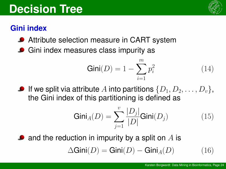
Gini indexAttribute selection measure in CART systemGini index measures class impurity as

Gini(D) = 1−m∑i=1

p2i (14)

If we split via attribute A into partitions {D1, D2, . . . , Dv},the Gini index of this partitioning is defined as

GiniA(D) =v∑j=1

|Dj||D|

Gini(Dj) (15)

and the reduction in impurity by a split on A is

∆Gini(D) = Gini(D)−GiniA(D) (16)

Support Vector Machines

Karsten Borgwardt: Data Mining in Bioinformatics, Page 25

Hyperplane classifiersVapnik et al. define a family of classifiers for binary clas-sification problems.This family is the class of hyperplanes in some dot prod-uct space H,

〈w, x〉 + b = 0, (17)

where w ∈ H, b ∈ R.These correspond to decision functions (‘classifiers’):

f (x) = sgn(〈w, x〉 + b) (18)

Vapnik et al. proposed a learning algorithm for deter-mining this f from the training dataset

Support Vector Machines

Karsten Borgwardt: Data Mining in Bioinformatics, Page 26

The optimal hyperplanemaximises the margin of separation between any train-ing point and the hyperplane

maxw∈H,b∈R

min{‖x− xi‖|x ∈ H, 〈w, x〉 + b = 0, i = 1, . . . ,m}(19)

Support Vector Machines

Karsten Borgwardt: Data Mining in Bioinformatics, Page 27

Optimisation problem

minimisew∈H,b∈R τ (w) =1

2‖w‖2 (20)

subject to yi(〈w, xi〉 + b) ≥ 1 for all i = 1, . . . ,m

Why minimise 12‖w‖

2?The size of the margin is 2

‖w‖. The smaller ‖w‖, thelarger the margin.Why do we have to obey the constraints yi(〈w, xi〉+b) ≥1? They ensure that all training data points of the sameclass are on the same side of the hyperplane and out-side the margin.

Support Vector Machines

Karsten Borgwardt: Data Mining in Bioinformatics, Page 28

The LagrangianWe form the Lagrangian:

L(w, b, α) =1

2‖w‖2 −

m∑i=1

αi(yi(〈xi, w〉 + b)− 1) (21)

The Lagrangian is minimised with respect to the primalvariables w and b, and maximised with respect to thedual variables αi.

Support Vector Machines

Karsten Borgwardt: Data Mining in Bioinformatics, Page 29

Support VectorsAt optimality,

∂

∂bL(w, b, α) = 0 and

∂

∂wL(w, b, α) = 0 (22)

such thatm∑i=1

αiyi = 0 and w =m∑i=1

αiyixi (23)

Hence the solution vector w, the crucial parameter of theSVM classifier, has an expansion in terms of the trainingpoints and their labels.Those training points with α > 0 are the Support Vec-tors.

Support Vector Machines

Karsten Borgwardt: Data Mining in Bioinformatics, Page 30

The dual problemPlugging (23) into the Lagrangian (21), we obtain thedual optimization problem that is solved in practice:

maximiseα∈RmW (α) =m∑i=1

αi −1

2

m∑i,j=1

αiαjyiyj〈xi, xj〉

(24)

The kernel trickThe key insight is that (24) accesses the training dataonly in terms of inner products 〈xi, xj〉We can plug in an inner product of our choice here! Thisis referred to as a kernel k:

k(xi, xj) = 〈xi, xj〉 (25)

Support Vector Machines

Karsten Borgwardt: Data Mining in Bioinformatics, Page 31

Some prominent kernelslinear kernel

k(xi, xj) =n∑l=1

xilxjl = x>i xj, (26)

polynomial kernel

k(xi, xj) = (x>i xj + c)d, (27)

where c, d ∈ R,Gaussian RBF kernel

k(xi, xj) = exp(− 1

2σ2‖xi − xj‖2), (28)

where σ ∈ R.

References and further reading

Karsten Borgwardt: Data Mining in Bioinformatics, Page 32

References

[1] B. Schölkopf and A. Smola. Learning with Kernels. MITpress, 2002.

[2] J. Han and M. Kamber. Data Mining: Concepts andTechniques. Elsevier, Morgan-Kaufmann Publishers,2006.

The end

Karsten Borgwardt: Data Mining in Bioinformatics, Page 33

See you tomorrow! Next topic: Clustering