Dassarma Final Tods

A

Consistent Thinning of Large Geographical Data for MapVisualization

Anish Das Sarma, Hongrae Lee, Hector Gonzalez, Jayant Madhavan, Alon HalevyGoogle Research{anish,hrlee,hagonzal,jayant,halevy}@google.com

Large-scale map visualization systems play an increasingly important role in presenting geographicdatasets to end users. Since these datasets can be extremely large, a map rendering system often needsto select a small fraction of the data to visualize them in a limited space. This paper addresses the funda-mental challenge of thinning: determining appropriate samples of data to be shown on specific geographicalregions and zoom levels. Other than the sheer scale of the data, the thinning problem is challenging becauseof a number of other reasons: (1) data can consist of complex geographical shapes, (2) rendering of dataneeds to satisfy certain constraints, such as data being preserved across zoom levels and adjacent regions,and (3) after satisfying the constraints, an optimal solution needs to be chosen based on objectives such asmaximality, fairness, and importance of data.

This paper formally defines and presents a complete solution to the thinning problem. First, we expressthe problem as an integer programming formulation that efficiently solves thinning for desired objectives.Second, we present more efficient solutions for maximality, based on DFS traversal of a spatial tree. Third,we consider the common special case of point datasets, and present an even more efficient randomized algo-rithm. Fourth, we show that contiguous regions are tractable for a general version of maximality, for whicharbitrary regions are intractable. Fifth, we examine the structure of our integer programming formulationand show that for point datasets, our program is integral. Finally, we have implemented all techniques fromthis paper in Google Maps [Google 2005] visualizations of Fusion Tables [Gonzalez et al. 2010], and wedescribe a set of experiments that demonstrate the tradeoffs among the algorithms.

Categories and Subject Descriptors: H.0 [Information Systems]: General—storage, retrieval; H.2.4[Database Management]: Systems

General Terms: Algorithms, Design, Management, Performance

Additional Key Words and Phrases: geographical databases, spatial sampling, maps, data visualization,indexing, query processing

1. INTRODUCTIONSeveral recent cloud-based systems try to broaden the audience of database users anddata consumers by emphasizing ease of use, data sharing, and creation of map andother visualizations [Esri 2012],[Vizzuality 2012],[GeoIQ 2012], [Oracle 2007], [Gon-zalez et al. 2010]. These applications have been particularly useful for journalists em-bedding data in their articles, for crisis response where timely data is critical for peoplein need, and are becoming useful for enterprises with collections of data grounded inlocations on maps [Cohen et al. 2011].

Map visualizations typically show data by rendering tiles or cells (rectangular re-gions on a map). One of the key challenges in serving data in these systems is that thedatasets can be huge, but only a small number of records per cell can be sent to thebrowser at any given time. For example, the dataset including all the house parcelsin the United States has more than 60 million rows, but the client browser can typi-cally handle only far fewer (around 500) rows per cell at once. This paper considers theproblem of thinning geographical datasets: given a geographical region at a particularzoom level, return a small number of records to be shown on the map.

In addition to the sheer size of the data and the stringent latency requirements onserving the data, the thinning problem is challenging for the following reasons:• In addition to representing points on the map, the data can also consist of complex

polygons (e.g., a national park), and hence span multiple adjacent map cells.

ACM Transactions on Database Systems, Vol. V, No. N, Article A, Publication date: January YYYY.

A:2

(a) Original viewpoint. (b) Violation of zoom consistency (c) Correct zoom in

Fig. 1. Violation of Zoom Consistency

Fig. 2. Violation of Adjacency Constraint

• The experience of zooming and panning across the map needs to be seamless, whichraises two constraints:• Zoom Consistency: If a record r appears on a map, further zooming into the

region containing r should not cause r to disappear. In other words, if a recordappears at any coarse zoom granularity, it must continue to appear in all finergranularities of that region.• Adjacency: If a polygon spans multiple cells, it must either appear in all cells it

spans or none; i.e., we must maintain the geographical shape of every record.Figure 1 demonstrates an example of zoom consistency violation. In Figure 1(a),

suppose the user wants to zoom in to see more details on the location with a ballonicon. It would not be natural if further zoom-in makes the location disappear as inFigure 1(b). Figure 2 shows an example of adjacency consistency violation for polygons.The map looks broken because the display of polygons that span multiple cells is notconsistent.


A:3

Even with the above constraints, there may still be multiple different sets of recordsthat can be shown in any part of the region. The determination of which set of pointsto show is made by application-specific objective functions. The most natural objectiveis “maximality”, i.e., showing as many records as possible while respecting the con-straints above. Alternatively, we may choose to show records based on some notion of“importance” (e.g., rating of businesses), or based on maximizing “fairness”, treatingall records equally.

This paper makes the following contributions. First, we present an integer program-ming formulation of size linear in the input that encodes constraints of the thinningproblem and enables us to capture a wide variety of objective functions. We show howto construct this program, capturing various objective criteria, solve it, and translatethe program’s solution to a solution of the thinning problem.

Second, we study in more detail the specific objective of maximality: we presentnotions of strong and weak maximality, and show that obtaining an optimal solutionbased on strong maximality is NP-hard. We present an efficient DFS traversal-basedalgorithm that guarantees weak maximality for any dataset, and strong maximalityfor datasets with only point records.

Third, we consider the commonly occurring special case of datasets that only con-sist of points. We present a randomized algorithm that ensures strong maximality forpoints, and is much more efficient than the DFS algorithm.

Fourth, we consider datasets that consist only of “contiguous” regions. We show thatthe intractability of strong maximality is due to non-contiguous regions. We presenta polynomial-time algorithm for strong maximality when a dataset consists only ofcontiguous regions.

Fifth, we perform a detailed investigation of the structure of our integer program-ming formulation. We show the result that when the dataset contains only points, theprogramming formulation is in fact integral, leading to an efficient, exact solution.

Finally, we describe a detailed experimental evaluation of our techniques over large-scale real datasets in Google Fusion Tables [Gonzalez et al. 2010]. The experimentsshow that the proposed solutions efficiently select records respecting aforementionedconstraints.

Section 2 discusses the related area of cartographic generalization, and presentsother related work. The rest of the paper is organized as follows. Section 3 definesthe thinning problem formally. Section 4 describes the integer programming solutionto the thinning problem. Section 5 studies in detail maximality for arbitrary regions,and Section 6 looks at the special case of datasets with point regions. Section 7 looksat datasets with contiguous regions, and Section 8 studies the structure of the linearprogram, presenting an integral subclass. Experiments are presented in Section 9, andwe conclude in Section 10.

2. RELATED WORKWhile map visualizations of geographical data are used in multiple commercial sys-tems such as Google Maps1 and MapQuest2, we believe that ours is the first paper toformally introduce and study the thinning problem, which is a critical component insome of these systems. The closest body of related research work is that of cartographicgeneralization [Frank and Timpf 1994], [Puppo and Dettori 1995].

Cartographic generalization deals with selection and transformation of geographicfeatures on a map so that certain visual characteristics are preserved at different mapscales [Frank and Timpf 1994], [Shea and Mcmaster 1989], [Ware et al. 2003]. This

1http://maps.google.com2http://mapquest.com


A:4

work generally involves domain expertise in performing transformations while mini-mizing loss of detail (e.g., merging nearby roads, aggregating houses into blocks, andblocks into neighborhoods), and is a notoriously difficult problem [Frank and Timpf1994]. Our work can be used to complement cartographic generalization in two ways.First, it can filter out a subset of features to input into the generalization process, andsecond, it can select a subset of the transformed features to render on a map. For exam-ple, you could assign importance to road segments in a road network, use our methodto select the most important segments in each region, and then generalize those roadsthrough an expensive cartographic generalization process. A process related to thin-ning is spatial clustering [Han et al. 2001], which can be used to summarize a map bymerging spatially close records into clusters. A major difference in our work is impos-ing spatial constraints in the actual sampling of records.

Labeling in dynamic maps is a very similar problem [Petzold et al. 2003; Been et al.2006; Been et al. 2010], which studies the placement of labels in a dynamically gener-ated map to avoid overlaps among labels. The number of labels is typically assumedto be too large for displaying all of them in the limited space, and an appropriate se-lection, and placing of labels has to be performed at an interactive speed. Althoughthe dynamic map labeling problem is very similar to the proposed thinning problem,there are a few differences. Labels can be thought of as a special case of polygons inthe thinning problem, e.g., fixed sized rectangles given a zoom level. In the thinningproblem, polygons are zoom-invariant. That is, the zoom level only changes the level ofdetails of an absolute world. Whereas labels change their relative positions dependingon the zoom level. Moreover, its major constraint is on avoiding overlaps among labels,while for thinning, the major concern is on the number of objects per cell. In [Beenet al. 2006], a similar optimality of showing as many labels as possible over a contin-uous zoom level range is defined and a greed algorithm is shown to be optimal. Verysimilar consistencies (e.g., zoom consistency) are proposed as well. However, uniquepriorities among labels are assumed and the optimality is with regard to the priority,which greatly simplifies the problem. Approximation algorithms are studied in [Beenet al. 2010] and their approximation factors are provided. None of the above worksperformed experimental evaluation with real-world datasets.

The importance of consistency in map rendering or visualization was considered pre-viously in other studies as well, e.g., [Tryfona and Egenhofer 1997; Dix and Ellis 2002].Tryfona and Egnhofer proposed a systematic model for the constraints that must holdwhen geographic databases contain multiple views of the same geographic objects atdifferent levels of spatial resolution [Tryfona and Egenhofer 1997]. However, the con-sistency is on topological relations. That is, the study concerns actual change of shapesdepending on the level of details such as the transition from a region with discon-nected parts to an aggregated one whereas the proposed consistencies are on selectionof objects. The zoom consistency is also implicitly mentioned in [Dix and Ellis 2002].However, the proposed solution is to resample the data, which could be costly. Sincethe resampling may slow down interaction, authors employed visual effects such assmoothing transitions between datasets to ease the problem. In contrast, the proposedsolutions are able to respect the consistencies without resampling the dataset.

Dealing with Big Data is has long been acknowledged as a challenge in the visu-alization community, e.g., [Thomas and (Eds.) 2005]. In the ATLAS system, Chan et.al partitioned large time-series data into time units such as year, month, and dayand returned a fixed number of data points based on the level of data required [Chanet al. 2008]. Piringer et. al used a multithreading architecture to support interactiv-ity [Piringer et al. 2009]. They subdivided the visualization space into layers wheredata is processed separately and can be reused. Fisher et. al proposed a differentapproach: their system shows sufficiently trustworthy incremental samples to allow


A:5

users to make decisions without fully processing the data [Fisher et al. 2012]. Stolteet.al developed a system for describing and developing multiscale visualization thatsupports multiple zoom paths and both data and visualization abstractions [Stolteet al. 2003]. Data cubes are employed for data abstraction and multiple zoom paths.One of the proposed patterns, thematic maps, is applicable when visualizing geograph-ically varying dependent measures that can be summarized at multiple levels of details(such as county or state). This scheme can be thought of as pre-defining (selecting) ge-ographical objects based on zoom levels. Our work is more concerned about selectingwhich geographic items to show at different zoom levels based on visualization con-straints, and therefore complements the works described above.

Multiple studies have shown that clutter in visual representation of data can havenegative impact in user experience [Phillips and Noyes 1982], [Woodruff et al. 1998].The principle of equal information density from the cartographic literature states thatthe number of objects per display unit should be constant [Frank and Timpf 1994]. Theproposed framework can be thought of as an automated way to achieve similar goalswith constraints. DataSplash is a system that helps users construct interactive visual-izations with constant information density by giving users feedback about the densityof visualizations [Woodruff et al. 1998]. However, the system does not automaticallyselect objects or force constraints.

The vast literature on top-K query answering in databases (refer to [Ilyas et al.2008] for a survey) is conceptually similar since even in thinning we effectively wantto show a small set of features, as in top-K. However, work on top-K generally as-sumes that the ranking of tuples is based on a pre-defined (or at least independentlyassigned) score. However, the main challenge in thinning is that of picking the right setof features in a holistic fashion (thereby, assigning a “score” per region per zoom level,based on the objective function and spatial constraints). Therefore, the techniques fromtop-K are not applicable in our setting.

Spatial data has been studied extensively in the database community as well. How-ever, the main focus has been on data structures, e.g., [Guttman 1984], [Samet 1990],query processing, e.g., [Grumbach et al. 1998], [Hjaltason and Samet 1998], spatialdata mining, e.g., [Han and Kamber 2000] and scalability, e.g., [Patel et al. 1997];these are all largely orthogonal to our contributions. The spatial index in Section 3 canbe implemented with various data structures studied, e.g., [Guttman 1984], [Hilbert1891].

Sampling is a widely studied technique that is used in many areas [Cochran 1977].We note that our primary goal is to decide the number of records to sample, while theactual sampling is performed in a simple uniformly random process.

Finally, a large body of work has addressed the problem of efficiently solving opti-mization problems. We used Apache Simplex Solver for ease of integration with oursystem. Other powerful packages, such as CPLEX also may be used. The idea of con-verting an integer program into a relaxed (non-integer) formulation in Section 4.2 is astandard trick applied in optimization theory in order to improve efficiency (by poten-tially compromising on optimality) [Agmon 1954].

This manuscript is an extended version of the conference paper [Das Sarma et al.2012]. Beyond the conference paper, we present here two new fundamental resultson tractable subclasses of thinning: (1) Section 7 considers contiguous regions, withthe main result that strong maximality is in PTIME for contiguous regions; (2) Sec-tion 8 considers point datasets, and proves the integrality of our linear programmingformulation for point datasets. Apart from the two strong results in the new sectionsdescribed above, we’ve also expanded the conference paper by including proof sketchesfor all technical results; the conference version of the paper did not contain proofs.


A:6

R1

R2 R3

R4

R5

C (a)11

C13

C22

C42

C32

C23

C33

C43

(b)

Fig. 3. Running Example: (a) Spatial tree with Z = 3; (b) Regions shown at z = 3 for c21.

3. DEFINITIONSWe begin by formally defining our problem setting, starting with the spatial organiza-tion of the world, defining regions and geographical datasets (Section 3.1), and thenformally defining the thinning problem (Section 3.2).

3.1. Geographical dataSpatial Organization. To model geographical data, the world is spatially divided into

multiple cells, where each cell corresponds to a region of the world. Any region of theworld may be seen at a specific zoom level z ∈ [1,Z], where 1 corresponds to the coarsestzoom level and Z is the finest granularity. At zoom level 1, the entire world fits in asingle cell c11. At zoom level 2, c11 is divided into four disjoint regions represented by cells{c21, . . . , c24}; zoom 3 consists of each cell c2i further divided into four cells, giving a setof 16 disjoint cells c31, . . . , c

316, and so on. Figure 1(a) is a cell at z = 13, and Figures 1(b)

and (c) are cells at z = 14. In general, the entire spatial region is hierarchically dividedinto multiple regions as defined by the tree structure below.

Definition 3.1 (Spatial Tree). A spatial tree T (Z,N ) with a maximum zoom levelZ ≥ 1 is a balanced 4-ary rooted tree with Z levels and nodes N , with 4Z−1 nodes atlevel-Z denoted NZ = {cZ1 , . . . , cZ4Z−1}.

The nodes at each level of the tree correspond to a complete and disjoint cell decompo-sition of an entire region, represented as one cell at the root. Values of Z in most com-mercial mapping systems range between 10 and 20 (it is 20 for Google Maps [Google2005]).

Example 3.2. Figure 3(a) shows a spatial organization of a tree with Z = 3. Atzoom-level z = 1 the entire space is a single cell, which are divided into 4 cells at z = 2,and 16 at the finest zoom level of z = 3. (The figure only shows the z = 3 cells for thecell c21 at z = 2.)

Note that such a hierarchical division of a region into subregions corresponds to aspace-filling curve [Sagan 1994]. Thus, the nodes at a particular level in the spatialtree can be used for index range scans for a subregion, when ordered based on thespace-filling curve.

Regions and Span. A region corresponds to a part of the world. Since the finest gran-ularity of data corresponds to cells at zoom level Z, any region can be defined by asubset of cells at zoom level Z.


A:7

Definition 3.3 (Region and point region). A region R(S) over a spatial tree T (Z,N )is defined by a subset S ⊆ NZ , |S| ≥ 1. A region R(S) is said to be a point region iff|S| = 1.

Intuitively, the shape of a region is completely specified by the set of cells at zoomlevel Z it occupies. Details finer than the cells at zoom Z aren’t captured; for example,a region doesn’t ”partially” occupy a finest-granularity cell. We often refer to regionsthat span cells at different levels:

Definition 3.4 (Region Span). A region R(S) over spatial tree T (Z,N ) is said tospan a cell czi ∈ N iff ∃cZj ∈ NZ such that cZj ∈ S and czi is an ancestor of cZj in T .We use span(R) to denote the set of all cells R spans.

Note that a region defined by a set of finest-granularity cells in the maximum zoomlevel spans every ancestor cell of these finest-granularity cells.

Example 3.5. Figure 3(b) shows 5 regions for the cell c21, showing their spans atz = 3 over cells c31, . . . , c

34. Although the regions are shown in “circular” shapes for clar-

ity, these regions conform to Definition 3.3: Regions R1, R2, and R3 are point regionsspanning only a single cell at z = 3 (and three cells each across the three zoom levels),and R4 and R5 span two cells at z = 3 (and 4 cells in aggregate: two each at z = 3 andone each at z = 1, 2).

Geographical Dataset. A geographical dataset (geoset, for short) consists of a set ofrecords, each describing either a point or a polygon on a map. For the purposes of ourdiscussion it suffices to consider the regions occupied by the records. Specifically, (1) arecord describing a point can be represented by a point region, and (2) a record describ-ing a polygon p can be represented by the region defined by set of finest-granularityregions in NZ that p occupies. In practice, we represent the actual points and poly-gons in addition to other structured data associated with the location (e.g., restaurantname, phone number).

Definition 3.6 (GeoSet). A geoset G = {R1, . . . , Rn} over spatial tree T (Z,N ) is aset of n regions over T corresponding to n distinct records. Ri represents the region ofthe record with identifier i.

3.2. The thinning problemWe are now ready to formally introduce the thinning problem. We start by describingthe constraints that a solution to thinning must satisfy (Section 3.2.1), and then moti-vate some of the objectives that go into picking one among multiple thinning solutionsthat satisfy the constraints (Section 3.2.2).

3.2.1. Constraints. To provide a seamless zooming and panning experience on the map,a solution to the thinning problem needs to satisfy the following constraints:1. Visibility: The number of visible regions at any cell czi is bounded by a fixed con-

stant K.2. Zoom Consistency: If a region R is visible at a cell czi , it must also be visible at

each descendant cell cz′

i′ of czi that is spanned by R. The reason for this constraintis that as a user zooms into the map she should not lose points that are alreadyvisible.

3. Adjacency: If a region R is visible at a cell czi , it must also be visible at each cellczi′ spanned by R. This constraint ensures that each region is visible in its entiretywhen moving a map around (at the same zoom level), and is not “cut out” from some


A:8

cells and only partially visible. Note that adjacency is trivial for points but not forpolygons.

Example 3.7. Going back to the data from Figure 3, suppose we have a visibilitybound of K = 1, then at most one of R1 − R5 can be visible in c11, one of R1, R4 can bevisible at c31, and at most one of R2 − R5 can be visible in cell c33. Based on the zoomconsistency constraint, if R4 is visible in c11, then it must be visible in c21, c31, and c33. Theadjacency constraint imposes that R5 is visible in neither or both of c33 and c34.

A consequence of the zoom consistency and adjacency constraints is that every regionmust be visible at all spanned cells starting at some particular zoom level. We cantherefore define thinning as the problem of finding the initial zoom level at which eachrecord becomes visible.

PROBLEM 3.1 (THINNING). Given a geoset G = {R1, . . . , Rn} over a spatial treeT (Z,N ), and a maximum bound K ∈ N on the number of visible records in any cell,compute a function min-level M : {1, . . . , n} → {1, . . . ,Z,Z + 1} such that the followingholds:

Visibility Bound: ∀czj ∈ N , z ≤ Z, we must have |V isM (G,T, czj )| ≤ K, whereV isM (G,T, czj ) denotes the set of all visible records at cell czj whose min-level is setto at most z:

V isM (G,T, czj ) = {Ri|(czj ∈ span(Ri))&(M(j) ≤ z)}

Intuitively, the min-level function assigns for each record the coarsest-granularityzoom level at which the record will start being visible and continue to be visible inall finer granularities. (A min-level of Z + 1 means that record is never visible.) Bydefinition, assigning a single min-level for each record satisfies the Zoom Consistencyproperty. Further, the fact that we are assigning a single zoom level for each recordimposes the condition that if a record is visible at one spanned cell at a particularlevel, it will also be visible at all other spanned cells at the same level. Thus, the Adja-cency property is also satisfied. The first condition in the problem above ensures thatat any specific cell in the spatial tree T , at most a pre-specified number K of recordsare visible.

Example 3.8. Considering the data from Figure 3, with K = 1, we have several pos-sible solutions to the thinning solution. A trivial function M1(Ri) = 4 is a solution thatdoesn’t show any region on any of the cells. A more interesting solution is M2(R1) = 1,M2(R2) = 3, and M2(·) = 4 for all other regions. This solution shows R1 in its cell fromz = 1 itself, and R2 from z = 3. Another solution M3 is obtained by setting M3(R1) = 2above and M3(·) being identical to M2(·) for other regions; M3 shows R1 only startingat z = 2. Arguably, M2 is “better” than M3 since R1 is shown in more cells withoutcompromising the visibility of any other region; next we discuss this point further.

3.2.2. Objectives. There may be a large number of solutions to the thinning problemthat satisfy the constraints described above, including the trivial and useless one set-ting the min-level of every region to Z+1. Below we define informally certain desirableobjective functions, which can be used to guide the selection of a specific solution. In thenext section we describe a thinning algorithm that enables applying these objectives.1. Maximality: Show as many records as possible in any particular cell, assuming

the zoom consistency and adjacency properties are satisfied.2. Fairness: Ensure that every record has some chance of being visible in a particular

cell, if showing that record doesn’t make it impossible to satisfy the constraints.


A:9

3. Region Importance: Select records such that more “important” records have ahigher likelihood of being visible than less important ones. For instance, impor-tance of restaurants may be determined by their star rating, and if there are tworestaurants in the same location, the one with the higher rating should have agreater chance of being sampled.

Not surprisingly, these objectives may conflict with one another, as shown by our nextexample. We can define several other intuitive objectives not considered above (e.g.,respecting “spatial density”); a comprehensive study of more objectives is left as futurework.

Example 3.9. Continuing with our data from Figure 3 and thinning solutions fromExample 3.8, clearly M1 is not maximal. We shall formally define maximality later,but it is also evident that M3 is not maximal, as M2 shows a strictly larger numberof records. Fairness would intuitively mean that if possible every record should havea chance of being visible; furthermore, regions that have identical spans (e.g., R2 andR3) should have equal chance of being visible. Finally, if we consider some notion ofimportance, and suppose R2 is much more important than R3, then R2 should have acorrespondingly higher likelihood of being visible.

3.3. Outline of our solutionsIn Section 4 we show how to formulate the thinning problem as an integer program-ming problem in a way that expresses the different objectives we described above. InSection 5, we consider the maximality objective in more detail and show that whileone notion of maximality renders the thinning problem NP-hard, there is a weakerform of maximality that enables an efficient solution. Finally, in Section 6, we studythe special case of a geoset consisting of point records only. Table I provides a quickreference of the common notations we use throughout the paper.

Table I. Reference for common notations used in the paper.

Notation Meaning

cji ith cell at zoom level jT (Z,N ) Spatial tree with Z levels and nodes N

Nz Nodes at zoom level zR(S) Region R defined by cells S ⊆ NZ

span(R) Span of a region RV isM (G,T, czj ) Set of all visible records at cell czj

P(G) = {P1, . . . , Pl} Partitioning of G into equivalence class based on region spansvzq Variable for number of records from partition Pq with min-level z

We note that this paper considers a query-independent notion of thinning, whichwe can compute off-line. We leave query-dependent thinning to future work, but notethat zooming and panning an entire dataset is a very common scenario in practice. Wealso note that a system for browsing large geographical datasets also needs to addresschallenges that are not considered here such as simplification of arbitrary polygonsin coarser zoom levels and dynamic styling of regions based on attribute values (e.g.,deciding the color or shape of an icon).

4. THINNING AS INTEGER PROGRAMMINGIn this section we describe an integer program that combines various objectives fromSection 3.2 into the thinning problem: our program has linear constraints and we for-mulate multiple objective functions, some of which are non-linear. Section 4.1 describesthe construction of the integer program and Section 4.2 discusses solving it.


A:10

4.1. Constructing the integer programIn this section, we shall start by discussing how to model the constraints of thinning,which are the key aspect of encoding the thinning problem as described in Section 3.2.Subsequently, we present objective functions that may be used to pick among multiplethinning solutions.

4.1.1. Modeling constraints. Given an instance of the thinning problem, i.e., a geosetG = {R1, . . . , Rn} over a spatial tree T (Z,N ), and a maximum bound K ∈ N on thenumber of visible records in any cell, we construct an integer program P as follows (werefer to the construction algorithm by CPALGO, for Constraint Program Algorithm):Partition the records based on spans: We partition G into equivalence classesP(G) = {P1, . . . , Pl} such that: (a) ∪nq=1Pq = G; and (b) ∀q,∀Ri, Rj ∈ Pq : span(Ri) =span(Rj). For ease of notation, we use span(Pq) to denote the span of a record in Pq.These partitions are created easily in a single pass of the dataset by hashing the set ofcells spanned by each record.Variables of the integer program: The set of variables V in the program P is ob-tained from the partitions generated above: For each partition Pq, we construct Z vari-ables v1q , v

2q , . . . , v

Zq . Intuitively, vzq represents the number of records from partition Pq

whose min-level are set to z.Constraints: The set C of constraints are:

(1) Sampling constraints:

∀q : |Pq| ≥Z∑

z=1

vzq (1)

∀q∀z : vzq ≥ 0 (2)

∀q∀z : vzq ∈ Z i.e., vzq is an integer (3)Equation (1) ensures that the number of records picked for being visible at eachzoom level does not exceed the total number of records in the partition. Further,(|Pq|−

∑Zz=1 v

zq ) gives the number of records from Pq that are not visible at any zoom

level. Equations (2) and (3) simply ensure that only a positive integral numberof records are picked from each partition from each zoom level. (Later we shalldiscuss the removal of the integer constraint in Equation (3) for efficiency.) Notethat given a solution to the integer program we may sample any set of records fromeach partition Pq respecting the solution.

(2) Zoom consistency and visibility constraint: We have a visibility constraint foreach cell that is spanned by at least one record:

∀czj ∈ N :∑

q:czj∈span(Pq)

∑z∗≤z

vz∗

q ≤ K (4)

The constraint above ensures that at cell czj , at most K records are visible. The ex-pression on the left computes the number of records visible at czj : for each partitionPq spanning czj , only and all variables vz

∗

q correspond to visible regions. Note thatall vz

∗

q with z∗ strictly less than z are also visible at czj due to the zoom consistencycondition.

(3) Adjacency constraint: we do not need to add another constraint because theadjacency constraint is satisfied by the construction of the variable vzq itself: eachregion from Pq visible at zoom level z is visible at all cells spanned at level z.


A:11

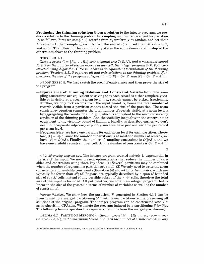
Producing the thinning solution: Given a solution to the integer program, we pro-duce a solution to the thinning problem by sampling without replacement for partitionPq as follows. First we sample v1q records from Pq uniformly at random and set theirM value to 1, then sample v2q records from the rest of Pq and set their M value to 2,and so on. The following theorem formally states the equivalence relationship of theconstraints above to the thinning problem.

THEOREM 4.1.Given a geoset G = {R1, . . . , Rn} over a spatial tree T (Z,N ), and a maximum bound

K ∈ N on the number of visible records in any cell, the integer program P(P,V, C) con-structed using Algorithm CPALGO above is an equivalent formulation of the thinningproblem (Problem 3.1): P captures all and only solutions to the thinning problem. Fur-thermore, the size of the program satisfies |V| = Z|P| = O(nZ) and |C| = O(nZ + 4Z).

PROOF SKETCH. We first sketch the proof of equivalence and then prove the size ofthe program:

— Equivalence of Thinning Solution and Constraint Satisfaction: The sam-pling constraints are equivalent to saying that each record is either completely vis-ible or invisible at a specific zoom level, i.e., records cannot be picked fractionally.Further, we only pick records from the input geoset G, hence the total number ofrecords visible from a partition cannot exceed the size of the partition. The zoomconsistency equation computes the total number of records visible at a zoom level zby aggregating the counts for all z∗ ≤ z, which is equivalent to the zoom consistencycondition of the thinning problem. And the visibility inequality in the constraints isequivalent to the visibility bound of thinning. Finally, as described earlier, we don’tneed to incorporate adjacency explicitly since we have just one variable per recordper zoom level.

— Program Size: We have one variable for each zoom level for each partition. There-fore, |V| = Z|P|; since the number of partitions is at most the number of records, wehave |V| = O(nZ). Finally, the number of sampling constraints is O(|nZ|), and wehave one visibility constraint per cell. So, the number of constraints is O(nZ + 4Z).

2

4.1.2. Minimizing program size. The integer program created naively is exponential inthe size of the input. We now present optimizations that reduce the number of vari-ables and constraints using three key ideas: (1) Several partitions may be combinedwhen the number of regions in a partition are small; (2) We only need to write the zoomconsistency and visibility constraints (Equation (4) above) for critical nodes, which aretypically far fewer than 4Z ; (3) Regions are typically described by a span of boundedsize of say M cells instead of any possible subset of the ∼ 4Z cells, therefore the totalsize of the input is bounded. All put together, we obtain an integer program that islinear in the size of the geoset (in terms of number of variables as well as the numberof constraints).

Merging Partitions. We show how the partitions P generated in Section 4.1.1 can betransformed to a merged partitioning Pm with fewer partitions while preserving allsolutions of the original program. The integer program can be constructed with Pm

as in Algorithm CPALGO. We denote the program induced by a partitioning P by P|P .The following lemma specifies the required conditions from the merged partitioning.

LEMMA 4.2 (PARTITION MERGING). Given a geoset G = {R1, . . . , Rn} over a spa-tial tree T (Z,N ), and a maximum bound K ∈ N on the number of visible records in any


A:12

Algorithm 1 An algorithm for the construction of a merged partition Pm (inducing asmaller but equivalent integer programming solution) from the output of AlgorithmCPALGO.

1: Input: (1) Geoset G = {R1, . . . , Rn} over spatial tree T (Z,N ), visibility bound K ∈N; (2) Output P, Cover(c), Touch(c) obtained from Algorithm CPALGO.

2: Output: Merged partitioning Pm.3: Initialize Pm = P, Stack S = root(T ) (i.e., the root node).4: while S 6= ∅ do5: Let node c = pop(S).6: // Check if c can be a valid merged partition root.7: if K ≥

∑P∈Touch(c) |P | then

8: Construct merged partition Pc = ∪P∈Cover(c)P .9: Set Pm = ({Pc} ∪ Pm) \ Cover(c).

10: else11: if c is not leaf then12: Push each child of c into S.

cell, the integer program P(P,V, C) over partitioning P = {P1, . . . , Pl}, P|P , is equiv-alent (i.e., have the same solutions) to the program P|Pm over a merged partitioningPm = {Pm

1 , . . . , Pmlm} where the following hold:

(1) Union: Each Pm ∈ Pm is a union of partitions in P, i.e., ∀Pm ∈ Pm∃S ⊆ P : Pm =⋃P∈S P

(2) Disjoint Covering: For Pm, Pn ∈ Pm, m 6= n⇒ (Pm∩Pn = ∅); and G =⋃

P∈Pm P(3) Size: Define span(Pm) = ∪Ri∈Pmspan(Ri). Let the span of any partition or region

restricted to nodes in zoom level Z be denoted spanZ ; i.e., spanZ(P ) = span(P )∩NZ .Then the total number of records overlapping with spanZ of any merged partitionis at most K: ∀Pm ∈ Pm : |{Ri ∈ G|spanZ(Ri) ∩ spanZ(P

m) 6= ∅}| ≤ K.

PROOF SKETCH. The disjoint covering condition ensures that each region is stillpart of exactly one partition. The union condition guarantees that the new set of parti-tions don’t “cover” different sets of region; rather, there is exactly one merged partitionthat is responsible for all regions from an original partition. Finally, the size conditionimposes the constraint that each merged partition overlaps with at most K regionsfrom the geoset; therefore, a solution based on the merged partitions can be mappedequivalently to a solution on the original set of partitions. 2

The intuition underlying Lemma 4.2 is that if multiple partitions in the originalprogram cover at most K records, then they can be merged into one partition withoutsacrificing important solutions to the integer program.

Algorithm 1 describes how to create the merged partitions. The algorithm uses twodata structures that are easily constructed during Algorithm CPALGO, i.e., in a singlepass of the data: (1) Cover(c), c ∈ N returning all original partitions from P whosespanned leaf nodes are a subset of the leaf nodes descendant from c; (2) Touch(c),c ∈ N returning all partitions from P that span some node in the subtree rooted at c.The algorithm constructs in a top-down fashion subtree-partitions, where each mergedpartition is responsible for all original partitions that completely fall under the sub-tree.

LEMMA 4.3. Given geoset G = {R1, . . . , Rn} over spatial tree T (Z,N ), visibilitybound K ∈ N, and the output of Algorithm CPALGO, Algorithm 1 generates a mergedpartitioning Pm that satisfies the conditions in Lemma 4.2 and runs in one pass of thespatial tree.


A:13

PROOF SKETCH. It is easy to see that Algorithm 1 traverses the spatial tree onlyonce, since it performs a depth-first traversal of the tree. Further, the algorithm con-structs a merged partition only if the size condition is satisfied; and since the mergedpartition is always constructed as a union of existing partitions, the Union conditionof Lemma 4.2 is satisfied. Finally, if a merged partition is constructed, Algorithm 1doesn’t traverse child nodes, thereby ensuring disjointness. 2

Constraints Only on Critical Nodes. We now show how to reduce the number of con-straints in the integer program by identifying critical nodes and writing constraintsonly for those nodes.

Definition 4.4 (Critical Nodes). Given a geoset G = {R1, . . . , Rn} over a spatial treeT (Z,N ), and a maximum bound K ∈ N on the number of visible records in any cell,and a set of (merged) partitions P = {P1, . . . , Pl} with corresponding spans of spanZ(as defined in Lemma 4.2), a node c ∈ N is said to be a critical node if and only if thereexists a pair of nodes cq1 ∈ spanZ(Pq1) and cq2 ∈ spanZ(Pq2), q1 6= q2, such that c is theleast-common ancestor of cq1 , cq2 in T .

Intuitively, a node c is a critical node if it is the least-common ancestor for at leasttwo distinct partitions’ corresponding cells. In other words, there are at least two par-titions that meet at c, and no child of c has exactly the same set of partition’s nodesin their subtree. Clearly we can compute the set of critical nodes in a bottom up passof the spatial tree starting with the set of (merged) partitions. Therefore, based onthe assignment of values to variables in the integer program, the total number of re-gions visible at c may differ from the number of nodes visible at parent/child nodes,requiring us to impose a visibility constraint on c. For any node c′ that is not a criticalnode, the total number of visible regions at c′ is identical to the first descendant criticalnode of c′, and therefore we don’t need to separately write a visibility constraint at c′.Therefore, we have the following result.

LEMMA 4.5 (CRITICAL NODES). Given an integer program P(P,V, C) over a(merged) set of partitions P as constructed using Algorithm CPALGO and Algorithm 1,consider the program P′(P,V, C′), where C′ is obtained from C by removing all zoom con-sistency and visibility constraints (Equation 4) that are not on critical nodes. We thenhave that P ≡ P′, i.e., every solution to P (P′, resp.) is also a solution to P′ (P, resp.).

PROOF SKETCH. The result follows from the fact that a constraint on any particularnode c ∈ N in the spatial tree is identical to the constraint on the critical node c′ ∈ N inc’s subtree with maximum height. That is, c′ is the critical node below c that is closestto c. Note that there is a unique closest critical node c′ below c: if not, c would havebeen a least-common ancestor and be a critical node itself. 2

Bounded Cover of Regions. While Definition 3.3 defines a region by any subset S ⊆NZ , we can typically define regions by a bounded cover, i.e., by a set of cover nodesC ⊆ N , where C is a set of (possibly internal) nodes of the tree and |C| ≤ M for somefixed constant M . Intuitively, the set S corresponding to all level-Z nodes is the setof all descendants of C. While using a bounded cover may require approximation of avery complex region and thereby compromise optimality, it improves efficiency. In ourimplementation we use M = 8, which is what is also used in our commercial offeringof Fusion Tables [Gonzalez et al. 2010]. The bounded cover of size M for every regionimposes a bound on the number of critical nodes.

LEMMA 4.6. Given a geoset G = {R1, . . . , Rn} with bounded covers of size M over aspatial tree T (Z,N ), the number of critical nodes in our integer programming formu-lation P is at most nMZ.


A:14

PROOF SKETCH. Every critical node of the tree must be an ancestor of some node inthe bounded cover of at least one region. Since there are at most nM bounded covers,there are at most nMZ nodes that are candidates for being critical nodes. 2

Summary. The optimizations we described above yield the main result of this section:an integer program of size linear in the input.

THEOREM 4.7. Given a geoset G = {R1, . . . , Rn} with a bounded cover of size Mover a spatial tree T (Z,N ), and a maximum bound K ∈ N on the number of visiblerecords in any cell, there exists an equivalent integer program P(P,V, C) constructedfrom Algorithms 1 and CPALGO with constraints on critical nodes such that |V| =Z|P| = O(nZ) and |C| = O(nMZ).

PROOF SKETCH. Follows from Theorem 4.1 and Lemmas 4.2, 4.3, 4.5, and 4.6. 2

4.1.3. Modeling objectives in the integer program. We now describe how objective functionsare specified. The objective is described by a function over the set of variables V.

To maximize the number of records visible across all cells, the following objectiveFmax represents the aggregate number of records (counting each record x times if it isvisible in x cells):

Fmax =∑czj∈N

∑q:czj∈span(Pq)

∑z∗≤z

vz∗

q (5)

Instead, if we wish to maximize the number of distinct records visible at any cell, wemay use the following objective:

Fdistinct =∑vzq∈V

vzq

The following objective captures fairness of records: it makes the total number ofrecords sampled from each partition as balanced as possible.

Ffair = −

∑Pq∈P

V (Pq)2

12

where V (Pq) =∑

z

∑z∗≤z v

z∗

q , i.e., we compute the number of records from Pq visibleat some cell czj , and aggregate over all cells. The objective above gives the L2 norm ofthe vector with V values for each partition. The fairness objective is typically best usedalong with another objective, e.g., Fmax + Ffair. Further, in order to capture fairnesswithin a partition, we simply treat each record in a partition uniformly, as we describeshortly.

To capture importance of records, we can create the optimization problem by subdi-viding each partition Pq into equivalence classes based on importance of records. Afterthis, we obtain a revised program P(P ′,V, C) and let I(Pq) denote the importance ofeach record in partition Pq ∈ P ′. We may then incorporate the importance into ourobjective as follows:

Fimp =∑czj∈N

∑q:czj∈span(Pq)

∑z∗≤z

I(Pq)vz∗

q (6)

Other objective functions, such as combining importance and fairness can be incor-porated in a similar fashion.


A:15

Example 4.8. Continuing with the solutions in Example 3.8 using data in Figure 3,let us also add another solution M4(·) with M4(R5) = 3, M4(R1) = 1 and M4(Ri) = 4for all other records. Further, suppose we incorporate importance into the records andset the importance of R2, R3 to 10, and the importance of every other record to 1.

Table II compares each of the objective functions listed above on all these solutions.Since M1 doesn’t show any records, its objective value is always 0. M2 shows twodistinct records R1 and R2, R1 shown in 3 cells, and R2 shown in one cell giving Fmax

and Fdistinct values as 4 and 2. Since M2 shows records in 3, 1, 0, and 0 cells fromthe partitions {R1}, {R2, R3}, {R4}, {R5} respectively, Ffair(M

2) = 20, and using theimportance of R2, we get Fimp = 13. Similarly, we compute the objective values forother solutions. Note that M4 is the best based on maximality, and M2 is the best basedon importance. Note that our objective of combining fairness, i.e., using Fmax + Ffair,gives M4 as the best solution. Finally, these solutions aren’t distinguished based onthe distinct measure.

Table II. Table comparing the objective measuresfor various solutions in Example 4.8.

Fmax Fdistinct Ffair Fimp

M1 0 0 0 0M2 4 2 -3.16 13M3 3 2 -2.24 12M4 5 2 -3.61 5

4.2. Relaxing the integer constraintsIn addition to the integer program described above, we also consider a relaxed programPr that is obtained by eliminating the integer constraints (Equation (3)) on vzq ’s. Therelaxed program Pr is typically much more efficient to solve since integer programsoften require exponential-time, and can be converted to an approximate solution. Wethen perform sampling just as above, except, we sample bvzqc regions. The resultingsolution still satisfies all constraints, but may be sub-optimal. Also, from the solution toPr, we may compute the objective values Fub(Pr), and the true objective value obtainedafter rounding down as above, denoted F(Pr). It can be seen easily that:

F(Pr) ≤ F(P) ≤ Fub(Pr)

In other words, the solution to Pr after rounding down gives the obtained value of theobjective, and without rounding down gives us an upper bound on what the integerprogramming formulation can achieve. This allows us to accurately compute potentialloss in the objective value due to the relaxation. Using this upper bound, in our exper-iments in Section 9, we show that in practice Pr gives the optimal solution in all realdatasets.

5. MAXIMALITYWe now consider the thinning problem for a geoset G = {R1, . . . , Rn}, with the specificobjective of maximizing the number of records shown, which is the objective pursuedby Fusion Tables [Gonzalez et al. 2010].3

3Our algorithms will satisfy restricted fairness, but maximality is the primary subject of this section.


A:16

5.1. Strong and weak maximalityMaximality can be defined as follows.

Definition 5.1 (Strong Maximality). A solution M : {1, . . . , n} → {1, . . . ,Z,Z + 1}to thinning for a geoset G = {R1, . . . , Rn} over a spatial tree T (Z,N ), and a maximumbound K ∈ N on the number of visible records in any cell is said to be strongly maxi-mal if there does not exist a different solution M ′ to the same thinning problem suchthat• ∀c ∈ N : |V isM (G,T, c)| ≤ |V isM ′(G,T, c)|• ∃c ∈ N : |V isM (G,T, c)| < |V isM ′(G,T, c)|The strong maximality condition above ensures that as many records as possible are

visible at any cell. We note that the objective function Fmax from Section 3.2.2 ensuresstrong maximality (but strong maximality doesn’t ensure optimality in terms of Fmax).

Example 5.2. Recall the data from Figure 3, and consider solutions M1,M2,M3

and M4 from Example 3.8 and 4.8. It can be seen that M4 is a strongly maximal solu-tion: All non-empty cells show exactly one region, and since K = 1, this is a stronglymaximal solution. Note that M2 (and hence M1 and M3) from Example 3.8 are notstrongly maximal, since c33 does not show any record and M4 above shows same num-ber of records as M2 in all other cells, in addition to c33.

Unfortunately, as the following theorem states, finding a strongly maximal solutionto the thinning problem is intractable in general.

THEOREM 5.3 (INTRACTABILITY OF STRONG MAXIMALITY). Given a geoset G ={R1, . . . , Rn} over a spatial tree T (Z,N ), and a maximum bound K ∈ N, finding astrongly maximal solution to the thinning problem is NP-hard in n.

PROOF SKETCH. We give a reduction from the NP-hard EXACT SET COVER prob-lem [Garey and Johnson 1979]: Given a universe U = {1, . . . , n} of n elements and afamily S = {S1, . . . , Sm} of subsets of U , determine if there exists a subset S∗ ⊆ S suchthat: (1) U =

⋃S∈S∗ S, (2) ∀Si, Sj ∈ S∗, Si 6= Sj ⇒ (Si ∩ Sj) = ∅.

Given an instance of the Exact Set Cover problem, we construct an instance of thethinning problem as follows: Construct a spatial tree with Z = dlog4 ne levels, n specialleaf nodes cZ1 , . . . , c

Zn . Also, we construct a geoset with m records G = {R1, . . . , Rm},

where the region of Ri is defined by exactly the set of leaf nodes corresponding toelements covered by Si: Ri spans cell cZj if and only if j ∈ Si. Finally, we set K = 1.

We claim that the strongly maximal solution to this instance of the thinning problemhas exactly one record visible at each of the n cells cZ1 , . . . , c

Zn : (1) Let S∗ be a solution

to the exact set cover problem; then we can set M(i) ≤ Z if and only if Ri ∈ S∗, and setM(i) = (Z + 1) otherwise. (The exact assignment of a value between 0 and Z for eachM(i) with Ri ∈ S∗ is irrelevant as we can just pick any arbitrary assignment ensuringall ancestors of each cZj , j ≤ n, have exactly one visible record. Note that this is astrongly maximal solution to thinning since all possible leafs (and all their ancestors)have exactly one record. (2) Conversely, if there is a solution M that ensures every leafnode cZj , j ≤ n has one visible record, then the sets corresponding to all these visiblerecords constitute a solution to the exact set cover problem. 2

Fortunately, there is a weaker notion of maximality that does admit efficient solu-tions. Weak maximality, defined below, ensures that no individual record can be madevisible at a coarser zoom level:

Definition 5.4 (Weak Maximality). A solution M : {1, . . . , n} → {1, . . . ,Z,Z + 1} tothinning for a geoset G = {R1, . . . , Rn} over a spatial tree T (Z,N ), and a maximum


A:17

bound K ∈ N on the number of visible records in any cell is said to be weakly maximalif for any M ′ : {1, . . . , n} → {1, . . . ,Z,Z + 1} obtained by modifying M for a singlei ∈ {1, . . . , n} and setting M ′(i) < M(i), M ′ is not a thinning solution.

Example 5.5. Continuing with Example 5.2, we can see that M2 (defined in Exam-ple 3.8) and M4 are weakly maximal solutions: we can see that reducing the M2 valuefor any region violates the visibility bound of K = 1. For instance, setting M2(R5) = 3shows two records in c34. Further, M3 from Example 3.8 is not weakly maximal, sinceM2 is a solution obtained by reducing the min-level of R1 in M3.

The following lemma expresses the connection between strong, weak maximality,and optimality under Fmax from Section 3.2.2.

LEMMA 5.6. Consider a thinning solution M : {1, . . . , n} → {1, . . . ,Z,Z + 1} for ageoset G = {R1, . . . , Rn} over a spatial tree T (Z,N ), and a maximum bound K ∈ N onthe number of visible records in any cell.• If M is optimal under Fmax, then M is strongly-maximal.• If M is strongly-maximal, then M is weakly-maximal.• If M is weakly-maximal and G only consists of point records, then M is strongly-

maximal.

PROOF SKETCH. We prove each part of the result separately:

— Suppose the solution based on Fmax is not strongly-maximal. Then based on the vio-lation of Definition 5.1, we can find a solution M ′ which has as many records visibleat every cell, and more records visible at at least one cell. Based on Theorem 4.1, M ′satisfies all constraints of the integer program. Since Fmax aggregates the counts ofeach cells, M ′ gives a higher objective value than M , leading to a contradiction.

— Follows directly from Definitions 5.1 and 5.4.— Suppose a dataset consisted only of points, and we have a weakly-maximal solution

M . Suppose that M is not strongly-maximal. Then based on Definition 5.1, thereexists some node c ∈ N in the strongly-maximal solution, for which fewer recordsare visible in the weakly-maximal solution. Let us consider such a cell c in moredetail. Consider the set of records V isM (G,T, c) visible at c based on the weakly-maximal solution M . To be able to increase the visibility count of this cell in thestrongly-maximal solution, there must be at least one region R 6∈ V isM (G,T, c) thatspans c. Since this region R is currently not visible in cell c, and the current visibilitycount at c is less than K (since the strongly-maximal solution increases its count),we can safely set M(i) to z, where z is the zoom level of c. This revision to M is aviolation of Definition 5.4.

2

5.2. DFS thinning algorithmThe most natural baseline solution to the thinning problem would be to traverse thespatial tree level-by-level, in breadth-first order, and assign as many records as al-lowed. Instead, we describe a depth-first search algorithm (Algorithm 2) that is expo-nentially more efficient, due to significantly reduced memory requirements. The mainidea of the algorithm is to note that to compute the set of visible records at a particu-lar node czj in the spatial tree, we only need to know the set of all visible records in allancestor cells of czj ; i.e., we need to know the set of all records from {Ri|czj ∈ span(Ri)}whose min-level have already been set to a value at most z. Consequently, we onlyneed to maintain at most 4Z cells in the DFS stack.


A:18

Algorithm 2 DFS algorithm for thinning.1: Input: Geoset G = {R1, . . . , Rn} over spatial tree T (Z,N ), visibility bound K ∈ N.2: Output: Min-level function M : {1, . . . , n} → {1, . . . ,Z + 1}.3: Initialize ∀i ∈ {1, . . . , n} : M(i) = Z + 1.4: Initialize Stack S with entry (c01, G).5: // Iterate over all stack entries (DFS traversal of T )6: while S 6= ∅ do7: Obtain top entry (czj , g ⊆ G) from S.8: Compute V isM (g, T, czj ) = {Ri ∈ g|(czj ∈ span(Ri))&&(M(i) ≤ z)}; let V Count =

|V isM (g, T, czj )|.9: // Sample more records if this cell is not filled up

10: if V Count < K then11: Let InV is = g \ V isM (g, T, czj ).12: // Sample up to SCount = min{(K − V Count), |InV is|} records from InV is.13: for Ri ∈ InV is (// in random order) do14: // Sampling Ri shouldn’t violate any visibility15: Initialize sample← true16: for cz ∈ span(Ri) do17: if V isM (G,T, cz) ≥ K then18: sample = false19: if sample then20: Set M(Ri) = z.21: if z < Z then22: // Create entries to add to the stack23: for Ri ∈ g do24: Add Ri to each child cell set gj corresponding cz+1

j for the children cells Ri

spans.25: Add all created (cz+1

j , gj) entries to S.26: Return M .

Algorithm 2 proceeds by assigning every record to the root cell of the spatial tree,and adding this cell to the DFS stack. While the stack is not empty, the algorithm picksthe topmost cell c from the stack and all records that span c. The required number ofrecords are sampled from c so as to obtain up to K visible records; then all the recordsin c are assigned to c’s 4 children (unless c is at level Z), and these are added into thestack. While sampling up to K visible records, we ensure that no sampled record Rincreases the visibility count of a different cell at the same zoom level to more than K;to ensure this, we maintain a map from cells in the tree (spanned by some region) totheir visibility count (we use V is to denote this count).

The theorem below summarizes properties of Algorithm 2.

THEOREM 5.7. Given a geoset G = {R1, . . . , Rn} over spatial tree T (Z,N ), andvisibility bound K ∈ N, Algorithm 2 returns:1. A weakly maximal thinning solution.2. A strongly maximal thinning solution if G only consists of records with point records.The worst-case time complexity of the algorithm is O(nZ) and its memory utilization isO(4Z).

(1) Correctness:— Weak Maximality: The weak-maximality of Algorithm 2 follows from the DFS

tree traversal: Every single cell c of the tree is considered before all of its de-


A:19

scendants. And when cell c is considered, as many records as possible are madevisible at the given cell. Therefore, no record at a descendant cell c′ can be madevisible at c (otherwise it would have been added when c was considered), givingus the necessary condition of Definition 5.4.

— Strong Maximality for Points: Follows from weak maximality andLemma 5.6.

(2) Complexity: Note that in a DFS traversal of a 4-ary tree with height Z, the stacksize never grows more than 4Z, giving the space requirement of 4Z. Also, note thateach record is considered once for every zoom level between 0 and Z, giving a timecomplexity of nZ.

2

The following simple example illustrates a scenario where Algorithm 2 does not re-turn a strongly maximal solution.

Example 5.8. Continuing with the data from Figure 3, suppose at z = 1 we ran-domly pick R1, and then at z = 3, we sample R2 from c34. We would then end up in thesolution M2, which is weakly maximal but not strongly maximal (as already describedin Example 5.5).

6. POINT ONLY DATASETSWe present a randomized thinning algorithm for a geoset G = {R1, . . . , Rn} consistingof only point records over spatial tree T (Z,N ).

The main idea used in the algorithm is to exploit the fact that no point spans multi-ple cells at the same zoom level: i.e., for any point record R over spatial tree T (Z,N ),if czj1 , c

zj2∈ span(R) then j1 = j2. Therefore, we can obtain a global total ordering of all

points in the geoset G, and for any cell simply pick the top K points from this globalordering and make them visible.

The algorithm (see Algorithm 3) first assigns a real number for every point indepen-dently and uniformly at random (we assume a function Rand that generates a randomreal number in [0, 1]; this random number determines the total ordering among allpoints). Then for every record we assign the coarsest zoom level at which it is amongthe top K points based on the total order.

To perform this assignment, we pre-construct a spatial index I : N → 2G, whichreturns the set of all records spanning a particular cell in the spatial tree T . That is,I(c) = {Ri|c ∈ span(Ri)}, and the set of records are returned in order of their randomnumber. This spatial index can be built in standard fashion (such as [Hilbert 1891;Guttman 1984]) in O(n log n) with one scan of the entire dataset. Assignment of thezoom level then requires one index scan.

THEOREM 6.1 (RANDOMIZED ALGORITHMS FOR POINTS). Given a geoset G ={R1, . . . , Rn} of point records over spatial tree T (Z,N ), spatial index I, and visibil-ity bound K ∈ N, Algorithm 3 returns a strongly maximal solution to the thinningproblem with an offline computation time O(n(Z + log n)), and constant (independentof the number of points) memory requirement.

PROOF SKETCH. It is easy to see that the solution returns a strongly maximal so-lution if it is a thinning solution: For each record we show up to K points if possible,so there is no room to increase the visibility count for any cell. The more subtle aspectof the result is the fact that the algorithm indeed returns a thinning solution, in par-ticular, that it satisfies the zoom consistency. To ensure zoom consistency, we note thatthe random number assignment gives a global priority ordering of all regions; hence,if a point has higher priority at some cell c, then it also have a higher priority at de-


A:20

Algorithm 3 A randomized thinning algorithm for geosets of point records.1: Input: Geoset G = {R1, . . . , Rn} of point records over spatial tree T (Z,N ), spatial

index I visibility bound K ∈ N.2: Output: Min-level function M : {1, . . . , n} → {1, . . . ,Z + 1}.3: Initialize ∀i ∈ {1, . . . , n} : M(i) = Z + 1.4: for i = 1 . . . n do5: Set priority(Ri) = Rand().6: for Non-empty cells czj ∈ I do7: K ′ = min{|I(czj )|,K}8: for Ri ∈ top-K ′(I(czj )) do9: if M(i) > z then

10: Set M(i) = z11: Return M .

scendant/ancestor cells, ensuring zoom consistency. Finally, the offline computation isperformed once for each point for each zoom level. 2

Furthermore, Algorithm 3 also has several other properties that make it especiallyattractive in practice.1. The second step of assigning M(i) for each i = 1..n doesn’t necessarily need to be

performed offline. Whenever an application is rendering the set of points on a map,it can retrieve the set of points in sorted order based on the random number, andsimply display the first K points it obtains.

2. One way of implementing the retrieval of first K points for a given cell is to applya post-filtering step after the index retrieval. In this case, the first step of randomnumber assignment can be performed online as well, completely eliminating offlineprocessing.

3. If we have pre-existing importance among records, the algorithm can use them todictate the priority assigned, instead of using a random number. For example, in arestaurants dataset, if we want to show more popular restaurants, we can assignthe priority based on the star-ratings of each restaurant (breaking ties randomly).

4. The algorithm can be extended easily to large geosets that don’t necessarily fit inmemory and are partitioned across multiple machines. The assignment of a randomnumber on each point happens independently and uniformly at random. Thereafter,each partition picks the top-K points for any cell based on the priority, and the over-all top-K are obtained by merging the top-K results from each individual partition.

7. CONTIGUOUS REGIONSSo far we have considered arbitrary regions (Definition 3.3) that may span any subsetof leaf cells in the spatial tree. In particular, regions may consist of cells from com-pletely different parts of the world. However, a common special case is that of “con-tiguous regions”, which represent regions that are not divided in space. In this section,we discuss how our results apply to the special case of contiguous regions.

A contiguous region over spatial tree T (Z,N ) with nodes at level-Z being NZ ={cZ1 , . . . , cZ4Z−1}may have a contiguous region that does not span consecutive cells fromNZ , as shown by the example below.

Example 7.1. Consider region R4 from Figure 3(b), which is contiguous in space.However, R4 would be represented using cells S4 = {c31, c33} based on Definition 3.3,which do not constitute a consecutive set of cells. Therefore, R4 is an example of aregion that is not contiguous based on Definition 3.3.


A:21

A complete characterization of the set of leaf cells that represent a contiguous regionis outside the scope of this paper. Instead, we use a simplified definition for contiguousregions:

Definition 7.2 (Contiguous Region). Consider a region R(S) over a spatial treeT (Z,N ) defined by a subset S ⊆ NZ , and let c ∈ N be the least common ancestorof nodes in S. We say that R(S) is a contiguous region if and only if ∀cZ descendant ofc, we have that cZ ∈ S.

We use the shorthand R∗(c) to denote the contiguous region R(S), where S is the setof all of c’s descendant leaf nodes in T (Z,N ).

Intuitively, a contiguous region R(S) (or R∗(c)) must be represented by a subset of cellsthat completely cover the leaf nodes of a subtree rooted at some internal node c. Nextwe investigate how contiguous regions affect the results obtained in the rest of thepaper.

We start by investigating the implications of contiguous regions on maximality (Sec-tion 7.1), and then briefly discuss the integer programming formulation (Section 7.2).

7.1. MaximalityOur main result of this section shows that when all regions are contiguous, strongmaximality is in PTIME. Contrast this with the NP-hardness for the general case(Theorem 5.3).

THEOREM 7.3 (TRACTABILITY OF STRONG MAXIMALITY). Given a geoset G ={R1, . . . , Rn} consisting of contiguous regions over a spatial tree T (Z,N ), and a maxi-mum bound K ∈ N, the problem of finding a strongly maximal solution to the thinningproblem is in PTIME.

In the following, we shall develop an algorithm that achieves strong maximality inpolynomial time, thereby proving the result. Let us start with a definition of “domina-tion” between a pair of contiguous regions. Recall we use the shorthand R∗(c) to denotea contiguous region defined by all leaf node descendants of an internal node c.

Definition 7.4 (Domination). Given contiguous regions R∗1(c1) and R∗2(c2) over spa-tial tree T (Z,N ), we say that R∗1(c1) dominates R∗2(c2) if c1 is an ancestor of c2 in T .

We have the following straightforward observation about domination of contiguousregions:

LEMMA 7.5 (DOMINATION). Given contiguous regions R∗1(c1) and R∗2(c2) over spa-tial tree T (Z,N ), if c1 6= c2, exactly one of the following properties holds:

(1) R∗1(c1) dominates R∗2(c2)(2) R∗2(c2) dominates R∗1(c1)(3) (span(R∗1(c1) ∩ span(R∗2(c2))) = ∅

PROOF SKETCH. Given two distinct nodes c1 and c2 in the spatial tree T , either c1is an ancestor of c2, or c2 is an ancestor of c1, or the subtrees rooted at c1 and c2 have adisjoint set of nodes. 2

The lemma above is based on the observation that if c1 6= c2, either c1 is an ancestor ofc2, or c2 is an ancestor of c1, or they don’t share any descendant.

Next we present a set of results on any thinning solution that enable us to obtain apolynomial-time algorithm:

LEMMA 7.6 (WEAK MAXIMALITY). Given a geoset G = {R1, . . . , Rn} consisting ofcontiguous regions over a spatial tree T (Z,N ), a maximum bound K ∈ N, and a thin-


A:22

ning solution M : {1, . . . , n} → {1, . . . ,Z,Z + 1}. Let the internal node defining Ri beczii , i.e., Ri is the contiguous region defined by an internal node ci at zoom level zi. Ifzi < M(i) < (Z + 1), then M is not weakly maximal.

PROOF SKETCH. Consider M ′ obtained from M as follows: (a) ∀j 6= i : M ′(j) =M(j), (b) M ′(i) = zi. We claim that M ′ is a thinning solution, thus violating the weakmaximality condition in Definition 5.4. A key observation to showing that M ′ is athinning solution is that when all regions are contiguous, we have that the number ofregions visible at any cell c is at most as many as those visible at some descendant c′

of c: This property holds because all regions that span c also span its descendant c′.Therefore, suppose M ′ violates the visibility bound of some cell c∗z′ , for z′ ≥ zi. Wecan now find a cell in M that also violates the visibility bound. Let the original valueof M(i) be x. Now, consider the descendant c∗x of c∗z′ at zoom level x: M must violatethe visibility bound of c∗x since all regions that are visible at c∗z′ based on M ′ are alsovisible at c∗x based on M , contradicting the fact that M is a thinning solution. 2

Intuitively, the result above says that when all regions are contiguous, any weak max-imal solution sets M(i) for a region Ri to be either Z +1 (i.e., not visible at all), or setsM(i) to at most zi (i.e., visible at all cells spanned by Ri). Therefore, finding a weaklymaximal thinning solution reduces to the problem of: (1) finding a maximal subsetGs ⊆ G = {R1, . . . , Rn} of regions, all of which are visible at each of the spanned cells,(2) restricting to records in Gs and finding any weakly maximal solution among them.The second step above can reuse the techniques from Section 5. Henceforth, we focuson Step (1) and simply use the shorthand M(Gs) to represent the thinning solutionwith: (a) ∀Ri ∈ Gs : M(i) ≤ zi as determined by Step (2), (b) M(i) = (Z + 1) otherwise.

We are now ready to present our main test for strong maximality.

THEOREM 7.7 (STRONG MAXIMALITY CONDITION). Given a geoset G ={R1, . . . , Rn} consisting of contiguous regions over a spatial tree T (Z,N ), a maxi-mum bound K ∈ N, a weakly maximal thinning solution M(Gs ⊆ G) is stronglymaximal if and only if the following condition holds: for any two distinct regionsRi ∈ Gs and Rj ∈ (G \Gs), Rj does not dominate Ri.

PROOF SKETCH. We prove the necessity and sufficiency in two parts:

— Only-if: Suppose that for some Ri ∈ Gs and Rj ∈ (G \ Gs), we have that Rj dom-inates Ri. Let Dom be the set of all regions in Gs such that for each R ∈ Dom: (1)Rj dominates R, (2) For any R′ 6= R, R′ ∈ Gs, R′ does not dominate R. Intuitively,Dom is the set of all regions in Gs dominated by Rj such that there are no domi-nation relationships among them; if there are two regions R and R′ dominated byRj , if R dominates R′, then only R is added to Dom. We have that the thinning so-lution M ′(Gs \ Dom ∪ {Rj}) violates the strong maximality of M . First, note thatM ′ is indeed a thinning solution: the set of regions in Dom collectively contributea visibility of at most 1 to each cell spanned by Rj . Further, Rj adds a visibility of1 to some extra nodes (e.g., those on the path from Ri to Rj), without violating thevisibility bound (as shown in Lemma 7.6).

— If: Next we show that if for any two distinct regions Ri ∈ Gs and Rj ∈ (G \ Gs), Rj

does not dominate Ri, then M(Gs) is strongly maximal if it is weakly maximal. Sup-pose M(Gs) is not maximal, consider a different strong maximal solution M ′(G′s).By Definition 5.1, we must have some cell c for which M ′ gives a higher visibilitycount than M . Consider the cell c in the thinning solution M(Gs). If we can obtain ahigher visibility on cell c, then there must be a region R∗(c∗) ∈ (G \ Gs) that spansc. Since M(Gs) is weakly maximal, adding R∗ to Gs violates the visibility of somecell c′ that is a descendant of c, since otherwise the same visibility bound of c would


A:23

Algorithm 4 An algorithm that returns a strongly-maximal thinning solution forgeosets of contiguous regions.

1: Input: Geoset G = {R1 ∗(cz11 ), . . . , Rn ∗(cznn )} of contiguous regions over spatial treeT (Z,N ), spatial index I visibility bound K ∈ N.

2: Output: Strongly-maximal Thinning Solution M(Gs)3: Initialize Gs ← ∅.4: Let ND be the non-dominated regions in (G \Gs)5: for R ∈ ND do6: if (adding R to Gs does not violate visibility) then7: Gs = Gs ∪ {R}8: Set ND to non-dominated regions in (G \Gs)9: Continue;

10: Return M .

have been violated. Since c′’s visibility bound is violated by including R∗(c∗) basedon some region R′ ∈ Gs that is dominated by R∗(c∗), the pair R′, R∗ violates thesufficiency condition of our theorem.

2

Based on Theorem 7.7, our goal is reduced to finding a maximal subset Gs ⊆ G ={R1, . . . , Rn} such that: (1) the visibility bound of all cells are satisfied; (2) no regionRi ∈ Gs is dominated by a region Rj ∈ (G \ Gs). We can obtain such a Gs by consid-ering regions in order of their domination strength: we start with regions that are notdominated by any other region and start including them into Gs as long as the visi-bility bound of cells is not violated. As regions are added into Gs, we keep consideringregions that are non-dominated in (G \ Gs). Algorithm 4 gives the basic pseudo-codefor this algorithm, where the computation of the non-dominated set of regions ND isdescribed in one step. In order to efficiently pick non-dominated regions from (G \Gs),we may create an efficient forest representation of the partial-order imposed by thedomination relationship; for instance, we may have a collection of binary search trees,with the comparator being the domination relationship. Details of this implementationare omitted.

We conclude by presenting the main result of this section.

THEOREM 7.8 (STRONG MAXIMALITY ALGORITHM). Given a geoset G ={R1, . . . , Rn} consisting of contiguous regions over a spatial tree T (Z,N ), and amaximum bound K ∈ N, Algorithm 4 returns a strongly-maximal solution M(Gs) tothe thinning problem in O(n(n+ Z)).PROOF SKETCHES OF THEOREMS 7.3 AND 7.8. Follows from Algorithm 4 and Theo-rem 7.7: Note that Algorithm 4 adds non-dominated regions whenever visibility is notviolated, ensuring weak maximality. Further, since any region R is added before everyregion R′ that R dominates, the condition of Theorem 7.7 is satisfied. 2

7.2. Integer programmingSince we have shown that strong maximality is achievable in polynomial-time, weconsider the integer programming only very briefly, describing how our results fromSection 4 change. Recall the definition of bounded covers from Section 4.1.2. By defini-tion, a contiguous region R ∗ (c) has a bounded cover of size 1 (the cover c). Therefore,we obtain the following corollary of Theorem 4.7:

COROLLARY 7.9. Given a geoset G = {R1, . . . , Rn} of contiguous regions over a spa-tial tree T (Z,N ), and a maximum bound K ∈ N on the number of visible records in


A:24

any cell, there exists an equivalent integer program P(P,V, C) constructed from Algo-rithms 1 and CPALGO with constraints on critical nodes such that |V| = Z|P| = O(nZ)and |C| = O(nZ).

PROOF SKETCH. Directly follows from Theorem 4.7 based on the fact that a contigu-ous region has a cover of size 1. 2

8. INTEGER PROGRAMMING FOR POINTSRecall, in Section 4.2 we considered a relaxed program Pr that is obtained by eliminat-ing the integer constraints (Equation (3)) on vzq ’s. The relaxation enabled us to solvethe problem efficiently sacrificing optimality, since integer programs are known to bemuch harder to solve than linear programs. This section closely explores the structureof our program to understand what makes the problem hard. In particular, the mainresult we develop in this section is to show that when our dataset consists only ofpoints, the relaxed linear program is in fact optimal.

To study properties of our linear relaxation of the integer program, we consider anequivalent form of the relaxed program Pr. Note that Pr is the same as P in Section 4.1except Cr, which does not have the integer constraints (Equation (3)). With the linearobjective functions in Section 4.1.3, we first define a linear program P′(P,W,Dr) fromPr(P,V, Cr) as follows.Variables of the transformed linear program: The set of variables W in the pro-gram P′ is obtained from the same partitions P: For each partition Pq, we constructZ variables w1

q , w2q , . . . , w

Zq , such that wz

q ≡∑z

z∗=1 vz∗

q . Intuitively, wzq represents the

number of records from partition Pq whose min-levels are smaller than or equal to z,that is, wz

q is the number of records from Pq that are visible at level z.

Constraints: The set Dr of constraints are:

wZq ≤ |Pq| (7)

∀q∀z < Z : wzq ≤ wz+1

q (8)∀q∀z : wz

q ≥ 0 (9)

∀czj ∈ N :∑

q:czj∈span(Pq)

wzq ≤ K (10)

To study this linear program, we define a specific encoding of the above linear pro-gram using the following matrix notation.

Definition 8.1 (Matrix Representation of P′(P,W,Dr)). We define P′(P,W,Dr) inmatrix notation as follows.

maximize F = cTw

subject to Aw ≤ b

and w ≥ 0

A is the constraint matrix enumerating: (1) constraints on the variable size (Con-straints (7) ∼ (9)) in ascending order of q and z, and then (2) constraints on the cells(Constraint (10)) in ascending order of z. With this construction, w and b are as follows:

w = (w11, w

21, · · · , wZ1 , w1

2, · · · , wZ2 , · · · , w1|P|, · · · , w

Z|P|)

T ,

b = (0, 0, · · · , |P1|, 0, · · · , |P2|, · · · , 0, · · · , |P|P||,K, · · · ,K)T .


A:25

cT is a vector of coefficients that defines F .

Let w∗ be a solution of P′, and v∗ be the corresponding solution of Pr. The followingequation gives v∗ from w∗:

v∗ = Lw∗

where L is a lower triangular matrix whose main diagonal entries are +1, entries rightbelow them are −1. All other entries are 0.

To understand the structure of A, we define partitions of it, based on the constraintsthey represent:

Definition 8.2 (Partitioning of A). We partition A vertically into two submatricesB and C. B is the upper block of A corresponding to constraints on variable size (Con-straints (7) ∼ (9)). C is the lower block of A corresponding to constraints on cells (Con-straints (10)).

A =

(B

C

)Example 8.3. Figure 4 presents a structural overview of A. Submatrices B and C

are distinguished by double horizontal lines. Single lines are to help identify blocksby q and z. ‘?’ represents that the value can be either 0 or 1 depending on the specificinstance of the problem.

We make the following observations on the structure of A, which follow from theconstruction of A in Definition 8.1:

(1) B is a square matrix of order Z|P|.(2) B is an upper triangular matrix whose main diagonal entries are +1 and entries

right above them, except those at column jZ + 1, 1 ≤ j < |P|, are −1. All otherentries are 0.

(3) Each column of C has at most one +1, and all other entries are 0. This follows fromthe fact that z is fixed given a column and a point record can span only a single cellat level z.

We now state a classical result that connects the matrix representation to linearprogramming: A matrix M is totally unimodular if the determinant of every squaresubmatrix of M is 0, −1 or +1. Its important connection to linear programming isthat if the constraint matrix is totally unimodular and bounds are integral, solving acontinuous relaxation of the problem always yields an integral solution vector, if anyexists [Schrijver 1986].

We are now ready to state the main result of this section in the following theorem,whose proof involves showing that our constraint matrix A is totally unimodular basedon the properties (1) ∼ (3).

THEOREM 8.4 (OPTIMALITY OF LINEAR RELAXATION). If a geoset G ={R1, . . . , Rn} consists of only point records, the relaxed linear program Pr definedin Section 4.2 is integral, and thus,

F(Pr) = F(P)where P is the integer programming formulation.

PROOF SKETCH. Consider an arbitrary square submatrix A′ of A. The goal is toprove det(A′) ∈ {±1, 0}, and thus A′ is totally unimodular. We prove this by inductionon the order t of A′. The base case of t = 1 is trivial so we assume t > 1.

Case 1: A′ has a column with only zeros, then det(A′) = 0.


A:26

A =

1 −1 · · · 0 0 · · · 0 · · · 0 · · · 00 1 −1 · · · 0 0 · · · 0 · · · 0 · · · 0...

.... . .

......

. . .... · · ·

.... . .

...0 0 · · · 1 0 · · · 0 · · · 0 · · · 00 0 · · · 0 1 −1 · · · 0 · · · 0 · · · 00 0 · · · 0 0 1 · · · 0 · · · 0 · · · 0...

.... . .

......

. . ....

. . ....

. . ....

0 0 · · · 0 0 · · · 1 · · · 0 · · · 0...

.... . .

......

. . ....

. . ....

. . ....

0 0 · · · 0 0 0 · · · 0 · · · 1 −1 · · · 00 0 · · · 0 0 0 · · · 0 · · · 0 1 · · · 0...

.... . .

......

. . ....

. . ....

. . ....

0 0 · · · 0 0 · · · 0 · · · 0 · · · 1

? 0 · · · 0 ? · · · 0 · · · ? · · · 00 ? · · · 0 0 ? · · · 0 · · · 0 ? · · · 00 ? · · · 0 0 ? · · · 0 · · · 0 ? · · · 00 ? · · · 0 0 ? · · · 0 · · · 0 ? · · · 00 ? · · · 0 0 ? · · · 0 · · · 0 ? · · · 0...

.... . .

......

. . ....

. . ....

. . ....

0 0 · · · ? 0 0 · · · ? · · · 0 0 · · · ?0 0 · · · ? 0 0 · · · ? · · · 0 0 · · · ?...

.... . .

......

. . ....

. . ....

. . ....

0 0 · · · ? 0 0 · · · ? · · · 0 0 · · · ?

Fig. 4. Structure of the constraint matrix A from Definitions 8.1 and 8.2

Case 2: A′ has a column with exactly one non-zero. After permuting rows andcolumns we have

A′ =

(±1 aT

0 A′′

)for some vector a and matrix A′′. By the induction hypothesis, det(A′′) ∈ {±1, 0}, hencedet(A′) ∈ {±1, 0}.

Case 3: Each column of A′ has two or more non-zeros. We show that this case doesnot exist from our construction of A.

Suppose that A has a square submatrix A′ such that all columns have at least twonon-zeros. First, we claim that A′ is not a submatrix of either B or C. Suppose A′ is asubmatrix of B and its order is t. We note that A′ cannot have any empty row (rowswith only zeros) since there are at least 2t non-zeros in A′ from the assumption, whichrequires at least t non-empty rows. This is because rows of B have at most two non-zeros (2t/2 = t). Thus, A′0,0 must be −1 for its first column to have two non-zeros, andthe first row has a single non-zero. We observe that the last row of A′ also has a singlenon-zero, i.e. +1, otherwise the last column cannot have at least two non-zeros. Sincethere are at least two rows with a single non-zero, the number of rows of A′ must beat least t+ 1 = (2t− 2)/2 + 2. This contradicts that A′ is a square matrix, and thus A′

cannot belong to B. Each column of C has at most a single +1, thus C cannot containA′ which has at least two non-zeros at all of its columns.


A:27

Second, suppose A′ spans both B and C. We show that A′ has at least t rows inB, which contradicts that A′ is a square matrix. Pick g, g ≤ t, columns in any singlevertical block that represents variables of the same record (c.f. Figure 4). If those gcolumns don’t have any non-zero in C, with the similar reasoning as above, they occupyat least g + 1 rows in B. If there is a column which spans C, they occupy at least grows in B since the column needs at least one non-zero in B and the rows that spanthem can overlap with other rows with non-zeros. Since rows with non-zeros in B fromdifferent vertical blocks are distinct, A′ has at least t rows in B and A′ cannot be asquare matrix.

Since any square submatrix in A has a determinant of 0 or ±1, A is totally unimod-ular and this concludes the proof. 2

The implication of Theorem 8.4 is that we can obtain an efficient solution for pointdatasets without hurting optimality: we just need to solve the linear program, whichis typically much more efficiently solvable than integer programs. We shall empiri-cally illustrate the general equivalence of the two programs for specific datasets inSection 9.3.

9. EXPERIMENTSThis section presents a detailed experimental evaluation of our algorithms. After pre-senting our datasets and experimental setup in Section 9.1, we present the followingmain experimental findings:1. In Section 9.2, we show that the optimization program minimization techniques

from Section 4.1.2 usually reduce the size of the problem by more than two ordersof magnitude.

2. In Section 9.3, we show that in all seven of our datasets, the integer relaxation(Section 4.2) doesn’t affect optimality as compared to the integer formulation.

3. Section 9.4 looks at scalability. The optimization program without minimizing pro-gram size scales only until around thousands of records, while after program-size minimization it scales to hundreds of thousands of records. A baseline tree-traversal algorithm scales to around ten million records, while our DFS traversalalgorithm scales to around 20 million records, after which they get bottlenecked bymemory.

4. In Section 9.5, we study objectives other than maximality, i.e., fairness and im-portance. First we show that for the importance-based objective of Fimp, the opti-mization program gives the best solution (as expected), but DFS also gives a closesolution. Further, we show that as skew in the importance increases, the value ofincorporating importance into the objective also increases. Then we present a qual-itative study of how fairness ensured by the optimization program’s objective im-proves the thinning solution by sampling records from regions in a roughly uniformfashion.

5. Finally, Section 9.6 gives a breakup of the optimization solution, showing that mostof the time is spent in building, and solving the problem, while sampling after thatis negligible.

The main takeaways from the experiments are: (1) When we care about maximalityonly, then the DFS algorithm presents a high-quality and efficient solution; (2) Forall other objectives, the optimization program along with the problem minimizationtechniques from this paper present a practical solution.


A:28

9.1. Experimental setupWe used the following real-world datasets containing points, lines and polygons, andtheir sizes varying from a few thousand records to more than 60 million. All the fol-lowing datasets are real data uploaded to our commercially-used Fusion Tables sys-tem [Gonzalez et al. 2010].

Name Type # records # pointsTheft point 2,526 2,526Flu point 6,776 6,776

U.S. county polygon 3,241 32,046Hiking Trails line 5,211 399,387

Ecoregion polygon 14,458 3,933,974Trajectory point 716,133 716,133U.S. Parcel point 61,924,397 61,924,397

These datasets describe: (1) the locations of motor vehicle thefts in Colier County, (2)the pharmacies and clinic locations in U.S. offering Flu vaccines, (3) the polygons ofall counties in the U.S., (4) popular hiking and biking trails in the world, (5) the set ofeco-regions in the world [Olson et al. 2001], (6) points from trajectories of individualsof a location-based social networking service, (7) the set of all housing parcels in theU.S.

We implemented and evaluated the following algorithms. The first three are basedon the integer programming solution, the next three are DFS and its variations, andthe final one is the randomized algorithm for points.• Optnaive is the integer program but without our proposed optimizations from Sec-

tion 4.1.2. Each record forms a single partition.• Optmax is the algorithm described in Section 4 with objective Fmax in Equation (5).• Optimp is the algorithm described in Section 4 with objective Fimp in Equation (6).

Importance of a record is a number between 0 and 1; we experimented with im-portance chosen uniformly at random for each record, as well as using a zipfiandistribution. We discretize the range and create equivalence classes by subdividingit into 10 buckets: (0, 0.1], (0.1, 0.2], ... (0.9, 1).

• DFS implements Algorithm 2, i.e., a depth-first search.• BFS is a baseline algorithm that is similar to Algorithm 2, but instead traverses

the spatial tree in a level-by-level fashion, starting from the root, then sampling forevery node in the root’s children, and so on.

• DFSimp is the same as DFS, but performs weighted sampling based on the recordimportance.

• Rand is Algorithm 3, which works for point datasets.We use Optnaive only to demonstrate how well the optimization framework can scalewithout the minimization technique. We implemented Rand with a post-filtering stepthat selects first K points at a cell as described in Section 6. That is, given a cell torender, we retrieve points that belong to the cell from I, assign numbers uniformly atrandom (but deterministically to maintain consistency across independent views), andselect the first K points. Since Rand only needs to assign random numbers to recordsand does not involve any thinning overhead, we do not include figures from Rand. Randconsumes only a constant memory and scales well to arbitrarily large datasets.


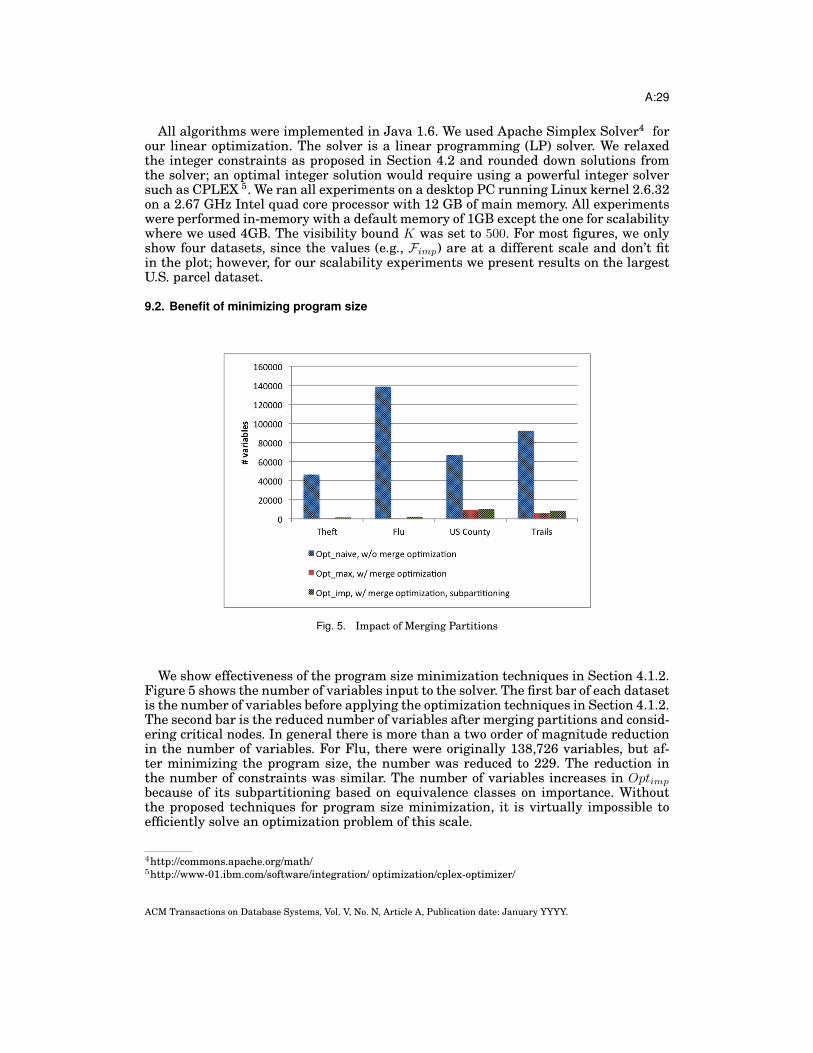
A:29

All algorithms were implemented in Java 1.6. We used Apache Simplex Solver4 forour linear optimization. The solver is a linear programming (LP) solver. We relaxedthe integer constraints as proposed in Section 4.2 and rounded down solutions fromthe solver; an optimal integer solution would require using a powerful integer solversuch as CPLEX 5. We ran all experiments on a desktop PC running Linux kernel 2.6.32on a 2.67 GHz Intel quad core processor with 12 GB of main memory. All experimentswere performed in-memory with a default memory of 1GB except the one for scalabilitywhere we used 4GB. The visibility bound K was set to 500. For most figures, we onlyshow four datasets, since the values (e.g., Fimp) are at a different scale and don’t fitin the plot; however, for our scalability experiments we present results on the largestU.S. parcel dataset.

9.2. Benefit of minimizing program size

Fig. 5. Impact of Merging Partitions

We show effectiveness of the program size minimization techniques in Section 4.1.2.Figure 5 shows the number of variables input to the solver. The first bar of each datasetis the number of variables before applying the optimization techniques in Section 4.1.2.The second bar is the reduced number of variables after merging partitions and consid-ering critical nodes. In general there is more than a two order of magnitude reductionin the number of variables. For Flu, there were originally 138,726 variables, but af-ter minimizing the program size, the number was reduced to 229. The reduction inthe number of constraints was similar. The number of variables increases in Optimp

because of its subpartitioning based on equivalence classes on importance. Withoutthe proposed techniques for program size minimization, it is virtually impossible toefficiently solve an optimization problem of this scale.

4http://commons.apache.org/math/5http://www-01.ibm.com/software/integration/ optimization/cplex-optimizer/


A:30

(a) All algorithms

(b) BFS & DFS

Fig. 6. Scalability

9.3. Integer relaxationWe compared our integer program solution with the relaxed solution (Section 4.2).Although the relaxed solution can theoretically be sub-optimal, in all 7 datasets weobserved identical solutions (i.e., relaxed solutions had integral variable values), dueto largely non-conflicting spatial distributions of records, thereby behaving almost likepoint datasets (which we know is integral from Section 8). This shows that employingthe relaxed solution does not affect optimality (significantly).

9.4. ScalabilityWe study scalability using the US Parcel dataset, which is our largest dataset. Figure 6plots runtime versus the number of records. To properly show the scale, Figure 6(a)plots a small data size range (up to 100,000 records), and Figure 6(b) plots a largerdata size range (up to 20 million records) showing BFS and DFS. We stop plotting analgorithm if it takes more than 10 minutes or needed more than 4G of memory. It isobvious that Optnaive is not scalable at all. It shows very sharp increase in runtimefrom the beginning and cannot even handle thousands of records. Optmax performs


A:31

well until hundreds of thousands of records, but after that the problem solving timebecomes the bottleneck. Optimp generates more number of variables and constraints,and thus is slower than Optmax.BFS and DFS outperform the optimization-based techniques by a large margin. The

performance of BFS starts to degrade at around ten million records. This is largelydue to the cost of memory management. At each stage, the algorithm holds recordscorresponding to all nodes under processing, which can consume a large amount ofmemory. However, in DFS, there are at most Z nodes at any given time, so it is muchmore efficient. We observe that DFS scales fairly well up to 20 million records whileBFS fails to scale up to that many records.

However, even DFS does not scale up above tens of millions of records due to itsmemory requirement. For point datasets, Rand only consumes a constant amountmemory and can handle arbitrarily large datasets, including the Parcel dataset. Tohandle large polygon datasets, we are exploring algorithms that are distributed overmultiple machines. The details are left for future work.

9.5. Objectives

Fig. 7. Objective Based on Importance with Uniform Distribution

First we consider optimality in datasets with importance. Figure 7 shows Fimp val-ues of various algorithms. By optimizing for Fimp, we can see Optimp achieves thehighest objective value for all data sets. We note that the objective values of DFS andDFSimp are very close to that of Optmax, with DFSimp being better than DFS. Further,as shown in Figure 8, using a zipfian distribution for importance enhances the gap be-tween importance-based algorithms versus the importance-agnostic ones; in general,the more skew there is in data, the more important it is to consider importance in theobjective.

Our observation on Fmax is also very similar. Fmax of DFS is within 1% of Optmax

for all datasets. And we shall show shortly that the DFS solutions are very efficient;hence, we infer that for maximality, the DFS solutions is most appropriate.

We next present the impact of considering fairness. We qualitatively compare the re-sults of two different objective functions: Fmax and Fimp. Figure 9(a) shows the resultfrom maximizing Fmax at a particular zoom level where all of North America is on themap. The figure shows a thinning solution by representing each visible record usinga red dot. (The overlap of red dots is simply because of the rendering on the map.)


A:32

Fig. 8. Objective Based on Importance with Zipfian Distribution

(a) Flu with Fmax (b) Flu with Fimp

Fig. 9. Results with Different Objective Functions

Notice that the artifact of partitions are visible (as rectangular holes). This is becauseFmax only tries to maximize the sum, and may assign a large value to one variable aslong as the assignment does not hurt the goal. In the example, the solver assigned 0to variables corresponding to empty holes assigning high values to others. While Fmax

only cares about maximality, Fimp considers importance. As we assign importance uni-formly at random and subdivide each partition according to the importance, the solveris not likely to choose everything from one partition and nothing from the other. Fig-ure 9(b) depicts the result from Fimp with random importance. We can see points aremuch more naturally distributed without seeing artifacts of partitioning.

We note that using Fimp is one of many possible ways to consider fairness. The L2

norm or adding a term for minimizing deviation from the mean are other examples,some of which would require a more powerful solver such as CPLEX 6.

9.6. Optimization runtimeFigure 10 presents the break-down of runtime of each of the optimization programs.The build time includes creation of Cover and Touch data structures in Algorithm 1,and the solve time is the time taken by the solver to solve the LP. The sample time isthe time taken for actually applying the solution to

6http://www-01.ibm.com/software/integration/ optimization/cplex-optimizer/


A:33

Fig. 10. Breakup of Runtime

For Optmax and Optimp, we see a large fraction of the runtime is spent in buildingand solving the optimization program. Optimp is the slowest due to increased numberof variables from subpartitioning. For larger datasets, the problem solving is the dom-inating part. A more powerful solver, such as CPLEX, will reduce the runtime greatly.

10. CONCLUSIONSWe introduced and studied the thinning problem of efficiently sampling regions from ageographical dataset for visualization on a map. The main challenges in the thinningproblem are effectively balancing spatial constraints imposed by commercial maps sys-tems (such as zoom consistency, visibility bound, and adjacency) with objective criteria(such as maximality, fairness, and record importance), while scaling to tens of millionsof records. We introduced an optimization framework that captures all constraints,and any general objective function, and showed how to perform several improvementsto the base model to reduce the problem to linear size. As our next contribution, weconsidered the objective of maximality and showed intractability results, and moreefficient algorithms. We then considered the common case of points and showed an ef-fective randomized algorithm. Finally, we presented detailed experimental results onreal datasets in our commercial Fusion Tables system [Gonzalez et al. 2010], demon-strating the effectiveness of our techniques.

We believe the proposed work can be extended in many interesting directions. Querydependent thinning is one important future work. When a query selects a subset of fea-tures, depending on its selectivity, the pre-computed thinning result can look sparse.Showing more features by relaxing the thinning result is desirable in such cases. Wecan also improve the algorithm’s scalability even further by disk-based or distributedthinning algorithms. Another future direction is to apply our work on the continuouszoom case. One possible adaptation to the continuous case is to interpolate solutionsbetween two discrete zoom levels, selecting a subset of features from the difference offeatures between the two levels. Another possibility is to define the problem with con-tinuous zoom from the start, where cells in a hierarchy form a square pyramid in 3Dspace.


A:34

REFERENCESAGMON, S. 1954. The relaxation method for linear inequalities. Canadian Journal of Mathematics 5, 3,

388–414.BEEN, K., DAICHES, E., AND YAP, C.-K. 2006. Dynamic map labeling. IEEE Transaction on Visualization

and Computer Graphics 12, 5, 773 – 780.BEEN, K., NOLLENBURG, M., POON, S.-H., AND WOLFFD, A. 2010. Optimizing active ranges for consistent

dynamic map labeling. Computational Geometry 43, 3, 312 – 328.CHAN, S., XIAO, L., GERTH, J., AND HANRAHAN, P. 2008. Atlas: Maintaining interactivity while exploring

massive time series. In IEEE Symposium on Visual Analytics Science and TEchnology (VAST ’08). 59 –66.

COCHRAN, W. G. 1977. Sampling Techniques, 3rd Edition. John Wiley.COHEN, S., LI, C., YANG, J., AND YU, C. 2011. Computational journalism: A call to arms to database

researchers. In Proceedings of the Conference on Innovative Data Systems Research. 148 – 151.DAS SARMA, A., LEE, H., GONZALEZ, H., MADHAVAN, J., AND HALEVY, A. Y. 2012. Efficient spatial sam-

pling of large geographical tables. In Proceedings of the ACM SIGMOD International Conference on theManagement of Data. 193 – 204.

DIX, A. AND ELLIS, G. 2002. by chance enhancing interaction with large data sets through statistical sam-pling. In Proceedings of the Working Conference on Advanced Visual Interfaces. 167 – 176.

ESRI. 2012. Arcgis. http://www.esri.com/software/arcgis/index.html.FISHER, D., POPO, I., DRUCKER, S. M., AND SCHRAEFEL, M. 2012. Trust me, i’m partially right: Incremen-

tal visualization lets analysts explore large datasets faster. In Proceedings of the SIGCHI Conference onHuman Factors in Computing Systems. 1673 – 1682.

FRANK, A. U. AND TIMPF, S. 1994. Multiple representations for cartographic objects in a multi-scale tree -an intelligent graphical zoom. Computers and Graphics 18, 6, 823 – 829.

GAREY, M. R. AND JOHNSON, D. S. 1979. Computers and Intractability: A Guide to the Theory of NP-Completeness. W. H. Freeman & Co.

GEOIQ. 2012. Geocommons. http://geocommons.com/.GONZALEZ, H., HALEVY, A. Y., JENSEN, C. S., LANGEN, A., MADHAVAN, J., SHAPLEY, R., SHEN, W., AND

GOLDBERG-KIDON, J. 2010. Google fusion tables: web-centered data management and collaboration.In Proceedings of the ACM SIGMOD International Conference on the Management of Data. 1061–1066.

GOOGLE. 2005. Google maps. http://maps.google.com.GRUMBACH, S., RIGAUX, P., AND SEGOUFIN, L. 1998. The dedale system for complex spatial queries. In

Proceedings of the ACM SIGMOD International Conference on the Management of Data.GUTTMAN, A. 1984. R-trees: A dynamic index structure for spatial searching. In Proceedings of the ACM

SIGMOD International Conference on the Management of Data. 47–57.HAN, J. AND KAMBER, M. 2000. Data Mining: Concepts and Techniques. Morgan Kaufmann.HAN, J., KAMBER, M., AND TUNG, A. K. H. 2001. Spatial clustering methods in data mining: A survey.

Geographic Data Mining and Knowledge Discovery, 1 – 29.HILBERT, D. 1891. Uber die stetige abbildung einer linie auf ein flachenstuck. Math. Ann. 38, 459–460.HJALTASON, G. R. AND SAMET, H. 1998. Incremental distance join algorithms for spatial databases. In

Proceedings of the ACM SIGMOD International Conference on the Management of Data. 237–248.ILYAS, I. F., BESKALES, G., AND SOLIMAN, M. A. 2008. A survey of top-k query processing techniques in

relational database systems. ACM Computing Surveys 40, 4, 11–58.OLSON, D. M., DINERSTEIN, E., WIKRAMANAYAKE, E., BURGESS, N., POWELL, G., UNDERWOOD, E.,

D’AMICO, J., ITOUA, I., STRAND, H., MORRISON, J., LOUCKS, C., ALLNUTT, T., RICKETTS, T., KURA,Y., LAMOREUX, J., W.W.WETTENGEL, HEDAO, P., AND KASSEM, K. 2001. Terrestrial ecoregions of theworld: A new map of life on earth. BioScience 51, 933–938.

ORACLE. 2007. Oracle spatial. http://www.oracle.com/us/products/database/options/spatial/index.html.

PATEL, J., YU, J., KABRA, N., TUFTE, K., NAG, B., BURGER, J., HALL, N., RAMASAMY, K., LUEDER, R.,ELLMANN, C., KUPSCH, J., GUO, S., LARSON, J., DEWITT, D., AND NAUGHTON, J. 1997. Buildinga scalable geo-spatial dbms: Technology, implementation, and evaluation. In Proceedings of the ACMSIGMOD International Conference on the Management of Data. 336–347.

PETZOLD, I., GROGER, G., AND PLUMER, L. 2003. Fast screen map labeling - data structures and algo-rithms. In Proceedings of International Cartographic Conference. 288 – 298.

PHILLIPS, R. AND NOYES, L. 1982. An investigation of visual clutter in the topographic base of a geologicalmap. Cartographic Journal 19, 2, 122 – 131.


A:35

PIRINGER, H., TOMINSKI, C., MUIGG, P., AND BERGER, W. 2009. A multi-threading architecture to supportinteractive visual exploration. IEEE Trans. on Visualization and Computer Graphics 15, 6, 1113 – 1120.

PUPPO, E. AND DETTORI, G. 1995. Towards a formal model for multiresolution spatial maps. In Interna-tional Simposium on Large Spatial Database. 152–169.

SAGAN, H. 1994. Space-Filling Curves. Springer-Verlag.SAMET, H. 1990. The design and analysis of spatial data structures. Addison-Wesley Longman Publishing

Co., Inc.SCHRIJVER, A. 1986. Theory of Linear and Integer Programming. John Wiley.SHEA, K. AND MCMASTER, R. 1989. Cartographic generalization in a digital environment: When and how

to generalize. AutoCarto 9, 56–67.STOLTE, C., TANG, D., AND HANRAHAN, P. 2003. Multiscale visualization using data cubes. IEEE Transac-

tion on Visualization and Computer Graphics 9, 2, 176 – 187.THOMAS, J. AND (EDS.), K. A. C. 2005. Illuminating the Path: The Research and Development Agenda for

Visual Analytics. IEEE Computer Society Press.TRYFONA, N. AND EGENHOFER, M. J. 1997. Consistency among parts and aggregates: A computation

model. Transactions in GIS 1, 3, 189 – 206.VIZZUALITY. 2012. Cartodb. http://cartodb.com.WARE, M. J., JONES, C. B., AND THOMAS, N. 2003. Automated map generalization with multiple operators:

a simulated annealing approach. International Journal of Geographical Information Science 17, 8, 743– 769.

WOODRUFF, A., LANDAY, J., AND STONEBRAKER, M. 1998. Constant information density in zoomable in-terfaces. In Proceedings of the Working Conference on Advanced Visual Interfaces. 57–65.


Dassarma Final Tods

Documents

Transcript of Dassarma Final Tods