A

pMphsDstsp©

K

1

sfa2cafvc

hawd

0d

Available online at www.sciencedirect.com

Computers and Chemical Engineering 32 (2008) 1507–1522

Dantzig–Wolfe decomposition and plant-wide MPC coordination

Ruoyu Cheng a, J. Fraser Forbes a,∗, W.San Yip b

a Department of Chemical and Materials Engineering, University of Alberta, Edmonton, AB T6G 2G6, Canadab Suncor Energy Inc., Fort McMurray, AB T9H 3E3, Canada

Received 16 December 2005; received in revised form 11 July 2007; accepted 12 July 2007Available online 28 July 2007

bstract

Due to the enormous success of model predictive control (MPC) in industrial practice, the efforts to extend its application from unit-wide tolant-wide control are becoming more widespread. In general, industrial practice has tended toward a decentralized MPC architecture. Most existingPC systems work independently of other MPC systems installed within the plant and pursue a unit/local optimal operation. Thus, a margin for

lant-wide performance improvement may be available beyond what decentralized MPC can offer. Coordinating decentralized, autonomous MPCas been identified as a practical approach to improving plant-wide performance. In this work, we propose a framework for designing a coordinationystem for decentralized MPC which requires only minor modification to the current MPC layer. This work studies the feasibility of applyingantzig–Wolfe decomposition to provide an on-line solution for coordinating decentralized MPC. The proposed coordinated, decentralized MPC

ystem retains the reliability and maintainability of current distributed MPC schemes. An empirical study of the computational complexity is used

o illustrate the efficiency of coordination and provide some guidelines for the application of the proposed coordination strategy. Finally, two casetudies are performed to show the ease of implementation of the coordinated, decentralized MPC scheme and the resultant improvement in thelant-wide performance of the decentralized control system.

2007 Elsevier Ltd. All rights reserved.

Comp

fiacacdoynrof

eywords: Decentralized MPC; Coordination; Dantzig–Wolfe decomposition;

. Introduction

Model predictive control (MPC) strategies have gained greatuccess in a wide range of industrial applications. The MPCramework can be divided into a steady-state calculation andcontrol calculation (or dynamic optimization) (Kadam et al.,002; Qin & Badgwell, 2003). The goal of the steady-state cal-ulation is to determine the desired targets for output, input,nd state variables at a higher frequency than those computedrom local economic optimizers. The target calculation pro-ides optimal achievable set-points that are passed to controlalculation.

With considerable development effort in recent years, thereas been a trend to extend MPC to large-scale applications, such

s plant-wide control. Two commonly used strategies for plant-ide MPC control and optimization are centralized schemes andecentralized schemes. A fully centralized or monolithic MPC

∗ Corresponding author. Tel.: +1 780 492 0873; fax: +1 780 492 2881.E-mail address: fraser.forbes@ualberta.ca (J. Fraser Forbes).

wctoTpg

098-1354/$ – see front matter © 2007 Elsevier Ltd. All rights reserved.oi:10.1016/j.compchemeng.2007.07.003

lexity analysis

or an entire large plant is often undesirable and difficult, if notmpossible, to implement (Havlena & Lu, 2005; Lu, 2003). Suchscheme can exhibit poor fault-tolerance, require an expensiveentralized computational platform, and can be difficult to tunend maintain. Alternatively, in many chemical plants, large-scaleontrol problems are solved by a group of MPC subsystems viaecentralized schemes, in which each MPC controller takes caref a specified operating unit. This decentralized MPC schemeields the desired operability, flexibility and reliability, but mayot provide an appropriate level of performance. In this paper,eliability refers to the possibility that some control subsystemsr portions thereof are able to function when other subsystemsail.

Most MPC implementations, when considered in a plant-ide context, have a decentralized structure, with individual

ontrollers working in an autonomous manner without coordina-ion. Such a decentralized scheme can only provide the optimum

peration for each unit with respect to its own objective function.hus, this approach may lead to a significant deviation from thelant-wide optimum. Lu (2003) claims that “the estimated latentlobal benefit for a typical refinery is 2–10 times more than what

1 mical Engineering 32 (2008) 1507–1522

Moa

mpbunriitotctilMptcskMel

svsiwi

almnosLdpcta

2

d

mwt

efiensuifpio

c&nitnh

x

∑

wtrl

d(sgf

508 R. Cheng et al. / Computers and Che

PC by itself can capture”. The key to exploiting the potentialf decentralized control systems, yet still retaining its structurend advantages, is cooperation.

This potential benefit has garnered increasing interest ofany researchers. (Camponogara, Jia, Krogh, & Talukdar, 2002)

roposed a distributed MPC scheme, where local control agentsroadcast their states and decision results to every other agentnder some pre-specified rules and this procedure continues untilo agent needs to do so. Recently, coordination-based MPC algo-ithms were discussed in Venkat, Rawlings, and Wright (2004),n which augmented states are used to model interactions, tomprove plant-wide performance via the coordination of decen-ralized MPC dynamic calculation. One common characteristicf the above two schemes is that the coordination of decen-ralized or distributed MPC controllers is completed without aoordinator, and thus controllers stand at equal status withinheir negotiation. Alternatively, in Lu (2003), a cross-functionalntegration scheme was developed, in which a coordination “col-ar” performed a centralized target calculation for decentralized

PC. This idea matches the wide-spread belief among industrialractitioners (Scheiber, 2004) that the trend toward decentraliza-ion will continue until the control system consists of seamlesslyollabrating autonomous and intelligent nodes with a supervi-ory coordinator overseeing the whole process. There are twoey factors that determine the desirability of the coordinatedPC system: computational efficiency of the coordination strat-

gy to ensure a real-time solution; and required information flowoad throughout the plant communication network.

This work discusses a framework for the coordination ofteady-state MPC target calculation level, which aims to pro-ide a timely response to local or plant-wide disturbances andetpoint changes. The proposed approach exploits the exist-ng plant computing, communication, and information systemsith minimal modification, to provide significant performance

mprovement.In industrial practice, a variety of optimization methods are

pplied to solve MPC target calculation problems, among whichinear programming (LP) and quadratic programming (QP) are

ost commonly used (Qin & Badgwell, 2003). Many MPC tech-ology products use a linear program to do the local steady-stateptimization (e.g., the Connoisseur controller offered by Inven-ys, Inc.). In this paper, we discuss the plant-wide coordination ofP-based MPC target calculation by using the ideas drawn fromecentralized economic planning. The Dantzig–Wolfe decom-osition principle is studied and applied to the development ofoordination scheme. An empirical study of complexity illus-rates the feasibility of the proposed strategy for industrialpplications.

. Dantzig–Wolfe decomposition

The Dantzig and Wolfe (1960) decomposition principle isepicted in Fig. 1.

In this decomposition approach, a large-scale linear program-ing problem can be separated into independent subproblems,hich are coordinated by a master problem (MP). The solu-

ion to the original large-scale problem can be shown to be B

Fig. 1. Mechanism of D–W decomposition.

quivalent to solving the subproblems and the MP through anite number of iterations Dantzig and Thapa (2002). Withinach iteration, the MP handles the linking constraints that con-ect the subproblems, using information [fi, ui] supplied by theubproblems (note that fi is the objective function value andi is the solution of the ith subproblem). Then, the MP sends

ts solution [π, γi] as price multipliers to all the subproblemsor updating their objective functions. Subsequently, the sub-roblems with updated objective functions are re-solved. Theterative procedure continues until convergence to the solutionf the large-scale problem.

The Dantzig–Wolfe decomposition hinges on the theorem ofonvex combination and column generation techniques (Dantzig

Thapa, 2002; Lasdon, 2002). The theorem of convex combi-ation, or D–W transformation, states that an arbitrary point xn a convex polyhedral set X = {x|Ax = b, x ≥ 0} can be writ-en as a convex combination of the extreme points of X plus aonnegative linear combination of the extreme rays (normalizedomogeneous solutions) of X, or

=L∑

i=1

αiui +M∑

j=1

βjνj (1)

L

i=1

αi = 1, αi, βj ≥ 0 (2)

here ui and νi are the finite set of all extreme points andhe finite set of all normalized extreme homogeneous solutionsespectively. If the feasible region is bounded, we can reformu-ate the problem by using the extreme points only.

Although any large-scale linear program problem can beecomposed and solved by Dantzig–Wolfe decompositionChvatal, 1983), the approach is particularly powerful fortructured linear programs. Consider a block-wise linear pro-ramming problem that has been converted to Simplex standardorm

min z1 =p∑

i=1

cTi xi

p (3)

subject to∑i=1

Aixi = b0

ixi = bi, xi ≥ 0, i = 1, 2, . . . , p (4)

mical

wsonuoo

∑

ws

x

f

p

ccv

2

atintecc&

Ruiim

(

w

f

osfc

m

bnt

tslonntgeoc

l2atb[

wzmrt

R. Cheng et al. / Computers and Che

here (3) represents the linking constraints associated with p

ubproblems, and the constraints in (4) are the local constraintsf independent subproblems. Via the theorem of convex combi-ation, the master problem (MP) can be formulated as followssing the linking constraints in (3) and the convex combinationf extreme points from (4), assuming that the feasible regionsf subproblems are bounded1

min z2 =p∑

i=1

N(i)∑j=1

fijλij

subject top∑

i=1

N(i)∑j=1

pijλij = b0

(5)

N(i)

j=1

λij = 1, λij ≥ 0, i = 1, 2, . . . , p (6)

here N(i) represents the number of extreme points of the fea-ible region in the it Ith LP subproblem, and

i =N(i)∑j=1

λijuji (7)

ij = cTi uj

i (8)

ij = Aiuji (9)

with uji being the jth extreme point of ith subproblem.

The resulting master problem has fewer rows in the coeffi-ient matrix than the original problem; however, the number ofolumns in the MP is larger due to an increase in the number ofariables associated with the extreme points of all subproblems.

.1. Multi-column generation algorithms

For a large-scale problem, it can be a formidable task to obtainll the extreme points and formulate a full master problem. Ifhe MP is solved via the Simplex method, only the basic sets needed and it has the same number of basic variables as theumber of rows. Thus, we do not need to explicitly know allhe extreme points of subproblems. This leads to solving anquivalent problem, the restricted master problem (RMP), whichan be dynamically constructed at a fixed size by incorporatingolumn generation techniques (Dantzig & Thapa, 2002; Gilmore

Gomory, 1961).Assume that we have a starting basic feasible solution to the

MP and it has a unique optimum. The optimal solution providess with the Simplex multipliers [π, γ , γ , . . . , γ ] for the basis

1 2 p

n the current RMP, with π associated with (5) and γi with theth constraint in (6), respectively. Then, the subproblems are

odified and solved to find the priced-out column associated

1 Unbounded cases are discussed in Lasdon (2002) and Dantzig and Thapa2002).

J

λ

Engineering 32 (2008) 1507–1522 1509

ith λij:

ij = (cTi − πAi)u

ji − γi (10)

and the ith subproblem is

min z0i = (cT

i − πAi)xi

subject to Bixi = bi, xi ≥ 0(11)

Here we notice that only minor modification is made to eachptimizing subproblem, i.e., an augmented term containing sen-itivity information is introduced into each subproblem objectiveunction. An optimal solution is reached when the followingondition is satisfied:

ini,j

fij = mini

(z0i − γi) ≥ 0, i = 1, . . . , p (12)

A complete proof of the optimality and finite convergence cane found in Dantzig and Thapa (2002). When condition (12) isot satisfied, a column generation strategy is used to determinehe column or columns that will enter the basis of the RMP.

The coordination of subproblems can be regarded as a direc-ional evaluation procedure for the feasible extreme points of theubproblems, in which the RMP evaluates and selects subprob-em solutions under the guidance of some “rules”. The selectedr priced-out extreme points will be used to generate columnseeded for updating the RMP. The column generation tech-iques are the “rules” that show good performance in directinghe evaluation of subproblem feasible solutions. With columneneration techniques, instead of an exhaustive traversal of allxtreme points of the subproblems, usually only a small subsetf the extreme points are required to be evaluated during theoordination procedure.

Several column generation techniques can be found in theiterature. In the single-column generation scheme (Lasdon,002), the minimum objective function value of problem (12) isssumed to come from subproblem s (1 ≤ s ≤ p), i.e., the solu-ion xs(π) solves subproblem s. Then, the column to enter theasis is generated by

Asxs(π)

is

](13)

here is is a n-component vector with a “1” in position s anderos elsewhere. The generated column is associated with theost favorable subproblem (i.e., that with the most negative

educed cost). Thus, with single-column generation algorithm,he updated RMP can be expressed as

min z3 =p∑

i=1

∑Jbasis

fijλij + f ∗λ∗

subject top∑

i=1

∑Jbasis

pijλij + p∗λ∗ = b0

(14)

∑basis

λij + λ∗ = 1, i = 1, 2, . . . , p (15)

ij ≥ 0, λ∗ ≥ 0 (16)

1 mical Engineering 32 (2008) 1507–1522

wefuiRodt

tttbmamTc(

J

λ

rIfct(eItaddap

3

itW

o

beauecs

walbicdscttfd

3

cp

w(tt

510 R. Cheng et al. / Computers and Che

here the λij is the current basic variables and λ∗ is the variablentering the basis. The terms associated with λ∗ can be derivedrom (7) to (9) and (13), which contribute to the generated col-mn. Jbasis is an index set whose elements coorespond to thendices of subproblem feasible solutions, which are now in theMP basis. Particularly, in the above formulation, the numberf variables in the basis is |Jbasis| = m0 + p,2 which shows theimension of the basic set in the RMP is (m0 + p), where m0 ishe number of linking constraints in (3).

It should be noted that any other subproblem with a nega-ive reduced cost has the potential to generate a column to enterhe basis of the master problem (Lasdon, 2002). To take advan-age of other favorable subproblems, multiple columns coulde considered for generating a new RMP. Several variants ofulti-column generation techniques are discussed in Dantzig

nd Thapa (2002) and Lasdon (2002). In this work, we study theulti-column generation scheme suggested in Lasdon (2002).hus, to incorporate all potential favorable proposals, a “new”olumn is generated in the RMP for each subsystem by applying13):

min z4 =p∑

i=1

∑Jbasis

fijλij +p∑

i=1

f ∗i λ∗

i

subject top∑

i=1

∑Jbasis

pijλij +p∑

i=1

p∗i λ

∗i = b0

(17)

∑basis

λij + λ∗i = 1, i = 1, 2, . . . , p (18)

ij ≥ 0, λ∗i ≥ 0 (19)

The above problem has n more variables than constraints,ather than one more as in the single-column generation case.f we use the size of the coefficient matrix in Simplex standardorm to represent the size of the problem, the RMP with multi-olumn generation has a size of (m0 + p) × (m0 + p + p) whilehe RMP with single-column generation has a size (m0 + p) ×m0 + p + 1). One would expect a greater decrease in z4 throughvery iteration, and thus, a reduction in the number of iterations.t was discussed in Lasdon (2002) and verified by the computa-ional experiments (Cheng, Forbes, Yip, & Cresta, 2005) that thedvantage of having more columns in the RMP outweighs theisadvantage of increased RMP size. Since the Dantzig–Wolfeecomposition algorithm with multi-column generation showshigher computational efficiency, we adopt this approach in thisaper.

. Plant-wide MPC coordination

Generally, because the process plant is built by connectingndividual operating units, the plant model has block-wise struc-ure and the steady-state coefficient matrix is usually sparse.

ith appropriate structural transformation, we can obtain a

2 Here the notation “||” is used to denote the number of elements or the lengthf a data set as is common practice in computing science.

Y

y

wT

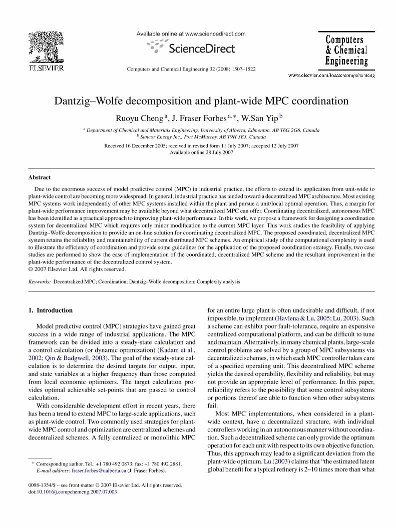
Fig. 2. Coordinated MPC target calculation.

lock-angular model with a small number of block off-diagonallements. The off-diagonal elements indicate the interactionsmong operating units. Most of the existing decentralized (e.g.,nit-wide) MPC controllers only consider the block-diagonallements of the plant-wide process model. Therefore, most pro-ess plants with decentralized MPC are potential candidates fortrategies to coordinate independent MPC.

Illustrated in Fig. 2 is a structural diagram of a typical plant-ide decentralized MPC structure. Note that each MPC containssteady-state target calculation and a dynamic control calcu-

ation (Ying & Joseph, 1999). A coordinator can be designedy considering different kinds of interactions among operat-ng units. Such interactions can be formulated as the linkingonstraints. Recall that the two key factors to efficient coor-ination are the computational efficiency of the coordinationtrategy and the required information flow throughout the plantommunication network. In the previous section we dealt withhe coordination, and in this section we are going to introducewo linking constraints construction approaches based on dif-erent interaction modeling methods, which ensure reasonableata traffic through the plant communication network.

.1. Approach 1: interstream consistency

For an individual MPC subsystem, which contains a targetalculation and a control calculation, we can formulate an LProblem, for the steady-state target calculation at time k as

min z = cTx(k)

subject to Aeqx(k) = beq(k), Lx(k) ≤ b(k)(20)

here x(k) = [us(k), ys(k)] is a vector of steady-state valuesi.e., targets or setpoints) for the input and output variables forhe subsystem. The equality constraints in (20) are taken fromhe linear dynamic model:

(s) = G(s)U(s) + Gd(s)D(s) + E(s) (21)

which yields the steady-state model

= Ku + Kdd + e (22)

here d are the disturbances and e is the unmeasured noise.he inequality constraints result from physical limitations on the

R. Cheng et al. / Computers and Chemical

irp(&p

mbtaeatn

dcAicfblsAaapc

3

iemcIv

sool

postpt

wCta

o

K

miaTis

Y

wul

y

e

wooswaw

i

Fig. 3. Demonstration of interstream consistency.

nputs and outputs, such as actuator limits or production qualityequirements. Other MPC target calculation formulations areossible, such as including model bias and soft output constraintsKassmann, Badgwell, & Hawkins, 2000; Lestage, Pomerleau,

Hodouin, 2002). These can easily be incorporated into theroposed method, but are omitted to simplify discussion.

The solution from the decentralized MPC target calculationay not be optimal with respect to the entire plant operation

ecause of plant/model mismatch, which results from ignoringhe interactions among operating units. In this case, the inter-ctions between two operating units can always be modeled byquating the appropriate output variables from the upstream unitnd the input variables to the downstream unit. Shown in Fig. 3,he hexagon labeled “A” represents the process interstream con-ecting individual operating units.

In formulating the subproblems, those streams connectingifferent operating units are torn and consistency relationshipsan be used to model the interactions between different units.ssume that we have p separate operation units, each of which

s controlled by one MPC subsystem. By introducing interpro-ess stream consistency as the linking constraints (3), we canormulate an LP problem that includes constraints (3) and (4)y incorporating those decentralized target calculation prob-ems. This problem has a block-wise structure which can beolved efficiently by Dantzig–Wolfe decomposition strategy.t each execution of the plant-wide MPC target calculation,coordinated LP problem will be updated and solved. Then

ll the calculated steady-state targets both for inputs and out-uts, including interprocess stream variables, are passed to MPControl calculation.

.2. Approach 2: off-diagonal element abstraction

Quite often, advanced control strategies are designed andmplemented at different times for different operating units. Forxample, in a copper ore concentrator plant, model-based and

odel-assisted APC controllers were separately installed in the

rushing, grinding and flotation sections (Herbst & Pate, 1996).n this case, certain controlled variables (CVs) and manipulatedariables (MVs) have been specified and grouped in a unit-wide

tvci

Engineering 32 (2008) 1507–1522 1511

ense. As we discussed before, these unit-based implementationf APC strategies can only use the block-diagonal informationf the plant model. Ignoring the off-diagonal information mayead to significant loss in the control performance.

Given the coordination mechanism of Dantzig–Wolfe decom-osition, if we can abstract off-diagonal elements from theverall plant model for the construction of the linking con-traints, the coordination only requires minor modifications tohe objective function and constraints of each decentralized MPCroblem. For the ith decentralized MPC system, the LP-basedarget calculation has the form:

min cTui

ui + cTyi

yi

subject to yi = Kiiui + ei, uilb ≤ ui ≤ ui

ub, yilb ≤ yi ≤ yi

lb

(23)

here ui and yi are the deviation variables for the MVs andVs, respectively. The vector ei represents the unmeasured dis-

urbances, uilb and yi

lb are the lower bounds, while uiub and yi

ubre the upper bounds for the decision variables.

If we have a full gain matrix for the entire plant with Nperating units

=

⎡⎢⎢⎢⎣

K11 K12 . . . K1N

K21 K22 . . . K2N

. . . . . . . . . . . .

KN1 KN2 . . . KNN

⎤⎥⎥⎥⎦ (24)

The matrix K can be ordered such that a unit-based imple-entation of MPC as in problem (23) uses the block-diagonal

nformation Kii of the plant model in its calculations. In suchcase, the off-diagonal blocks may be treated as disturbances.his way of dealing with the off-diagonal information can result

n undesirable closed-loop behavior, when the interactions areignificant. Assume the plant-wide model is

(k) = KU(k) + E(k) (25)

here Y (k) and U(k) are the CVs and MVs of N local operatingnits concatenated into vectors; E(k) is the concatenation ofocal disturbance variables (DVs). This is equivalent to

i(k) = Kiiui(k) + eim(k) + ei

u(k) (26)

im(k) −

N∑j=1

Kijuj(k) = 0 j �= i (27)

here the auxiliary variable eim, which is an abstraction of the

ff-diagonal elements, represents the influence of the inputs ofther operating units on the local system; ei

u stands for unmea-ured noise. In the proposed coordination scheme, a coordinatorill be developed to handle the constraints (27) and drive the

uxiliary variable eim to the values corresponding to the plant-

ide optimum operations. In this case, in each unit-based MPC

arget calculation, the auxiliary vector em is treated as a decisionariable, since Eq. (27) are not included in each unit-based MPCalculation. Thus, the decision variables in each individual MPCs augmented to [ui, yi, ei

m].

1 mical Engineering 32 (2008) 1507–1522

g[coscd

Rgcpiw(cdp1rware

4

idatt

a

B

x

wal

cadm

r

o

ab(

4

cpgmeppb(oscI

nwwaccptttatmcbb

512 R. Cheng et al. / Computers and Che

Furthermore, the objective function of each MPC systemets dynamically updated based on the sensitivity informationπ, γi], as in (10), from the solution of the master problem by theoordinator. After each execution of the optimization, only theriginal CVs or MVs will be implemented. The coordinationcheme is particularly efficient for coordinating decentralizedontrol systems based on plant-wide models with sparse off-iagonal matrices.

emark 1. Using the above two approaches, we are able toather interaction information that plays an important role in theoordination of decentralized MPC. Compared with the locallyrocessed information within a decentralized control system, thenformation flow traffic conveyed by the communication net-ork is not heavy. In this scheme, only the optimal solution

one feasible point and the objective function value) and theonstraints’ sensitivity information are passed between the coor-inator and each subsystem. For example, within the solution alant-wide MPC problem containing 10 linking constraints and00 decision variables from 5 subsystems, the information flowequired to be transmitted through the communication networkithin one communication cycle is less than 1000 bytes.3 In

ddition, for the off-diagonal element abstraction method, it mayequire additional efforts for the identification of off-diagonallements (gains).

. Complexity analysis

The computational efficiency of a coordination strategys a key factor in determining the viability of using coor-inated decentralized optimization approaches in industrialpplications. In the following sections, we evaluate the computa-ional efficiency of the Dantzig–Wolfe decomposition algorithmhrough an empirical complexity study.

Without loss of generality, we consider a large-scale block-ngular LP problem with p subproblems in its standard form

max∑

i

cTi xi

subject to∑

i

Aixi = b0

(28)

ixi = bi (29)

i ≥ 0 i = 1, 2, . . . , p (30)

here vectors xi (ni × 1), bi (mi × 1), b0 (m0 × 1), ci (ni × 1),nd matrices Ai (m0 × ni), Bi (mi × ni) are specific to subprob-em “i”.

Computational complexity is the study of determining theost of solving a numerical computing problem using a scientific

lgorithm. In this work, the cost of the proposed Dantzig–Wolfeecomposition approach can be interpreted as the required arith-etic or other computational operations.4 Although the cost of

3 For platforms that use double (64-bit) precision floating-point numbers toepresent a real number according to IEEE Standard 754 floating point.4 In this paper, the definition of an arithmetic operation, such as an additionr a multiplication, is applied to two real numbers.

t

au1mwt

Fig. 4. Worst-case behavior illustration.

n algorithm can be measured in several ways, the “worst-case”ehavior and “average-case” behavior are two typical measuresNash & Sofer, 1996).

.1. Worst-case behavior

Unlike a complete enumeration approach, the process ofoordination can be viewed as a directional evaluation of sub-roblem extreme points in the RMP. When the multi-columneneration technique is incorporated into a coordinated opti-ization scheme, shown in Fig. 4, the RMP (coordinator) will

valuate a new set of p extreme points submitted by each sub-roblem at every iteration. Note that the new set of p extremeoints in black is not generated by an arbitrary combinationut under the direction of coordinator (RMP). In Fig. 4, them0 + p) extreme point set in gray is associated with the RMPptimal basis at the previous coordination iteration. The p pointet is a new set of extreme points submitted by subproblems aturrent iteration, and Ni is the number of extreme points of theth subproblem feasible region.

The worst-case behavior analysis depends on the LP tech-iques that are used for solving the RMP and subproblems. Theorst-case behavior of Simplex methods is non-polynomial;hereas, the interior point methods are polynomial time

lgorithms. If Simplex methods are used and we take its worst-ase performance, the Dantzig–Wolfe decomposition algorithmannot be a polynomial time algorithm. Even though each sub-roblem can generate an (optimal) extreme point in polynomialime, using interior point methods (IPM), it may take exponen-ial time to get all the extreme points for a subproblem. Notehat each subproblem has mi constraints and ni decision vari-bles. Thus, the number of extreme points can be as many ashe combinationniCmi. Therefore, in the worst-case, whatever

ethods are used to solve either RMP or subproblems, theoordination process might theoretically evaluate every com-ination of the subproblem extreme points. Then, worst-caseehavior analysis for Dantzig–Wolfe decomposition implicateshat it may not be a polynomial time algorithm.

Usually, only when the worst-case behavior well reflects theverage-case behavior of an algorithm, is it used to provide anpper bound of the cost of solving a problem (Nash & Sofer,

996). For example, the worst-case performance of interior pointethods (IPM) gives a rather tight upper bound; however, aorst-case analysis does not reflect the observed performance of

he Simplex method (Chvatal, 1983; Nash & Sofer, 1996). Since

mical

ac

4

vs

T

ws(fTpim

T

T

soamistiuwlc

T

p

∃

(

taaacm

mib

4

pst

t

wloib

t

t

aea

t

wacctsc

t

R. Cheng et al. / Computers and Che

verage-case behavior is more relevant for our work, average-ase performance will be emphasized here.

.2. Average-case behavior

Considering the coordination mechanism discussed in pre-ious sections, the overall complexity for the decompositiontrategy can be expressed as

= {T(RMP) +p∑

i=1

T(SPi)} × CCN (31)

here T represents the number of arithmetic operations forolving the LP problem, and the communication cycle numberCCN) is used to distinguish the number of Simplex iterationsrom that of coordination iterations (the times to solve the RMP).hus, the required arithmetic operations are attributed to twoarts: the operations for solving the subproblems and the RMPn a single communication cycle, as well as the number of com-

unication cycles.If we define the first part as the non-coordination complexity:

(NonCo) = T(RMP) +p∑

i=1

T(SPi) (32)

the overall complexity can be expressed as

= T(NonCo) × CCN (33)

In the Simplex method, for an LP problem with m̄ con-traints and n̄ variables in standard form, the cost of solvingne iteration is O(m̄n̄) for Gaussian elimination plus O(m̄3)rithmetic operations for periodic re-factorization of the basisatrix,5 thus the arithmetic operation needed in one Simplex

teration is O(m̄3 + m̄n̄) (Nash & Sofer, 1996). Here, we con-ider the average-case performance of Simplex method6 andake the average number of Simplex iterations as O(m̄ + n̄) asn Andrei (2004). Therefore, the average behavior bound to besed is O(m̄4 + n̄m̄2 + m̄3n̄ + n̄2m̄) for the Simplex method,hich shows polynomial time complexity. For the LP prob-

em described in (28–30), we can derive the non-coordinationomplexity from

T(RMP) ∈ O(M40 + N0M

20 + M3

0N0 + N20M0) where

M0 = m0 + p, N0 = m0 + 2p (34)

and

(SPi) ∈ O(m4i + nim

2i + m3

i ni + n2i mi), i = 1, 2, . . . , p

(35)

Since the above numbers of arithmetic operations are allolynomials in corresponding m and n, the complexity of

5 The O() notation for a given function g(n) is given as O(g(n)) = {f (n) :a+ and n+

0 such that 0 ≤ f (n) ≤ ag(n) for all n ≥ n+0 }.

6 The observed scaling behavior of Simplex method is between m̄ and 3m̄

Nash & Sofer, 1996).

tLmrm

pt

Engineering 32 (2008) 1507–1522 1513

he non-coordination computation in (32) can be expresseds a polynomial with respect to the number of constraintsnd decision variables. In other words, the non-coordinationrithmetic operations T(NonCo) can be computed very effi-iently if we consider the average-case behavior of Simplexethod.The other part of the complexity analysis deals with the com-

unication cycles. To our knowledge, there is no similar analysisn the literature and therefore resort to a study of the averageehavior of CCN via a comprehensive empirical study.

.3. Empirical study of complexity

For analysis of the computational complexity of the decom-osition algorithm, since the algorithms are implemented on aequential machine, we may express the overall complexity inerms of computational time

=CCN∑

{t(RMP) +p∑

i=1

t(SPi)} (36)

here t represents the total computational time to solve a prob-em. Through the comparison between the computational timef each subproblem and the total computational time, we candentify and focus on the “bottleneck” subproblem, which maye the largest in dimension or hardest to solve.

Similarly, if we denote the non-coordination computationalime as

(NonCo) = t(RMP) +p∑

i=1

t(SPi) (37)

nd assume a distributed/parallel computing environment, forxample, one CPU for each subproblem, then we have the equiv-lent computational time (parallel computing)

eqv(NonCo) = t(RMP) + maxpi=1{t(SPi)} (38)

Such a distributed computing environment coincides withhat is encountered in current plant-wide decentralized MPC

pplications. In this case, it may be desirable to balance theomputational load on each computing node because the non-oordination computational complexity (teqv) relies heavily onhe largest subproblem. We will reemphasize this point in nextection. Then, the computational time within a decentralizedomputing environment can be expressed as

eqv =CCN∑

teqv(NonCo) (39)

Next the focus is on the analysis of CCN, where the rela-ionship between CCN and the characteristic parameters of theP problems such as m0, p, and |Ii| = (mi × ni) is to be deter-ined. Note that, each parameter may have physical meaning in

eal systems. For instance, in the plant-wide MPC coordination,0 may reflect the density of interactions among operating units;could be the number of decentralized MPC controllers or dis-

ributed industrial computers; while |Ii| can represent the size

1 mical Engineering 32 (2008) 1507–1522

ooibb

CDpaIpdt

(

(

(

w“

Aameawtp

{

sphlelc

•

•

central planning board may end up with less coordination iter-ations. Since the solution of a larger subproblem is more timeconsuming, Fig. 8 shows an increase in the computationaltime of Dantzig–Wolfe decomposition algorithm, but its per-

514 R. Cheng et al. / Computers and Che

f the control problems handled by an MPC subsystem. More-ver, the influence of the relative subproblem ratio (RSR), whichs defined as RSR = {max|Ii|/|Ij|, i, j = 1, 2, . . . , p}, will alsoe studied. The RSR gives some idea on the computational loadalance throughout the distributed computing network.

In the following Monte Carlo simulations, besides theCN, the computational efficiency and scaling behavior ofantzig–Wolfe decomposition will also be investigated by com-aring the performance between the decomposition algorithmnd the centralized LP solvers on the platform of MatLab®.n both solvers, ILOG® CPLEX 9.0 is used to solve all LProblems. In our study, we focus on the average behavior ofifferent optimization strategies in solving the problems withhe following assumptions:

1) No cycling: many techniques can be applied to efficientlydeal with cycling.

2) No degeneracy: when degeneracy occurs in practice, it canbe well handled using techniques such as perturbation tech-niques in Simplex method.

3) The studied problems have bounded feasible regions andoptimal solutions.

Due to the random nature of Monte Carlo simulation, weould like to acknowledge that there is possibility that an

average-case” problem may not be represented in our test set.The scheme of test problem generation is introduced in

ppendix A. It randomly generates a set of LP problems withblock-angular structure. We start from a reference problemodel, whose problem size and structure should be a good ref-

rence for the comparison experiments, i.e., we can observelgorithm performance changes when we change the problemith respect to the reference model. With some preliminary

ests, we choose the following set of parameters as the referenceroblem model:

p = 17, m0 = 30, mi = 40, ni = 30 . . . i = 1, 2, . . . , p}(40)

Note that the reference problem has subproblems of identicalize, i.e., the problem is thus a “well-balanced” decomposableroblem with RSR = 1. We also assume that each subproblemas been allocated to a distributed CPU. Therefore, the equiva-ent computational time teqv for the decomposition algorithm isstimated by summing up the time for solving the master prob-em and the most difficult subproblem, assuming a distributedomputational environment.

Scenario 1. We fix p and |Ii|, change m0 (see Appendix B).In this case, we can study the performance of decompositionand coordination with respect to the dimension of linkingconstraints in Eq. (28).

Fig. 5 shows that the CCN increases almost linearlywith the dimension of linking constraints increases. InFig. 6, when the number of linking constraints is small, thedecomposition algorithm gives comparable performance

Fig. 5. Coordination complexity.

to the centralized LP solver. When the number of linkingconstraints increases, the computational performance getsworse. This shows the computational complexity of thedecomposition algorithm has strong dependence on thedimension of linking constraints.

Scenario 2. For fixed it p and m0, we change subproblem size|Ii| by simultaneously changing mi and ni (see Appendix B).In this case, we study the algorithm performance with respectto subproblem sizes.

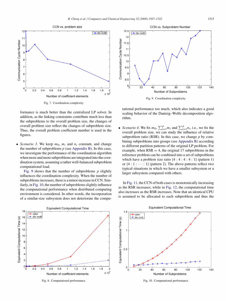
Fig. 7 shows a rather surprising result. Intuitively, one maythink that the CCN would increase when subproblem sizeincreases, because the overall problem gets bigger. By anal-ogy to the coordination of plants in a large company, largerplant proposals are usually less sensitive to coordination andthus do not tend to change dramatically. In such a case, the

Fig. 6. Computational performance.

R. Cheng et al. / Computers and Chemical Engineering 32 (2008) 1507–1522 1515

•

•

Fig. 7. Coordination complexity.

formance is much better than the centralized LP solver. Inaddition, as the linking constraints contribute much less thanthe subproblems to the overall problem size, the changes ofoverall problem size reflect the changes of subproblem size.Thus, the overall problem coefficient number is used in thefigures.

Scenario 3. We keep m0, mi and ni constant, and changethe number of subproblems p (see Appendix B). In this case,we investigate the performance of the coordination algorithmwhen more and more subproblems are integrated into the coor-dination system, assuming a rather well-balanced subproblemcomputational load.

Fig. 9 shows that the number of subproblems p slightlyinfluences the coordination complexity. When the number ofsubproblems increases, there is a minor increase in CCN. Sim-

ilarly, in Fig. 10, the number of subproblems slightly influencethe computational performance when distributed computingenvironment is considered. In other words, the incorporationof a similar-size subsystem does not deteriorate the compu-

Fig. 8. Computational performance.

aai

Fig. 9. Coordination complexity.

tational performance too much, which also indicates a goodscaling behavior of the Dantzig–Wolfe decomposition algo-rithm.

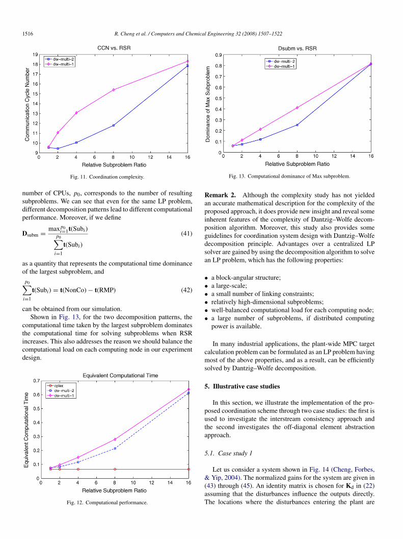
Scenario 4. We fix m0,∑p

i=1mi and∑p

i=1ni, i.e., we fix theoverall problem size, we can study the influence of relativesubproblem ratio (RSR). In this case, we change p by com-bining subproblems into groups (see Appendix B) accordingto different partition patterns of the original LP problem. Forexample, when RSR = 4, the original 17 subproblems in thereference problem can be combined into a set of subproblemswhich have a problem size ratio {4 : 4 : 4 : 4 : 1} (pattern 1)or {4 : 1 : · · · : 1} (pattern 2). The above patterns reflect twotypical situations in which we have a smaller subsystem or alarger subsystem compared with others.

In Fig. 11, the CCN of both cases is monotonically increasing

s the RSR increases; while in Fig. 12, the computational timelso increases as the RSR increases. Note that an identical CPUs assumed to be allocated to each subproblem and thus the

Fig. 10. Computational performance.

1516 R. Cheng et al. / Computers and Chemical Engineering 32 (2008) 1507–1522

nsdp

D

ao

∑c

cticd

Rapipgdsa

••••••

Fig. 11. Coordination complexity.

umber of CPUs, p0, corresponds to the number of resultingubproblems. We can see that even for the same LP problem,ifferent decomposition patterns lead to different computationalerformance. Moreover, if we define

subm = maxp0i=1t(Subi)

p0∑i=1

t(Subi)

(41)

s a quantity that represents the computational time dominancef the largest subproblem, and

p0

i=1

t(Subi) = t(NonCo) − t(RMP) (42)

an be obtained from our simulation.Shown in Fig. 13, for the two decomposition patterns, the

omputational time taken by the largest subproblem dominates

he computational time for solving subproblems when RSRncreases. This also addresses the reason we should balance theomputational load on each computing node in our experimentesign.

Fig. 12. Computational performance.

cms

5

puta

5

&(aT

Fig. 13. Computational dominance of Max subproblem.

emark 2. Although the complexity study has not yieldedn accurate mathematical description for the complexity of theroposed approach, it does provide new insight and reveal somenherent features of the complexity of Dantzig–Wolfe decom-osition algorithm. Moreover, this study also provides someuidelines for coordination system design with Dantzig–Wolfeecomposition principle. Advantages over a centralized LPolver are gained by using the decomposition algorithm to solven LP problem, which has the following properties:

a block-angular structure;a large-scale;a small number of linking constraints;relatively high-dimensional subproblems;well-balanced computational load for each computing node;a large number of subproblems, if distributed computingpower is available.

In many industrial applications, the plant-wide MPC targetalculation problem can be formulated as an LP problem havingost of the above properties, and as a result, can be efficiently

olved by Dantzig–Wolfe decomposition.

. Illustrative case studies

In this section, we illustrate the implementation of the pro-osed coordination scheme through two case studies: the first issed to investigate the interstream consistency approach andhe second investigates the off-diagonal element abstractionpproach.

.1. Case study 1

Let us consider a system shown in Fig. 14 (Cheng, Forbes,

Yip, 2004). The normalized gains for the system are given in

43) through (45). An identity matrix is chosen for Kd in (22)ssuming that the disturbances influence the outputs directly.he locations where the disturbances entering the plant are

R. Cheng et al. / Computers and Chemical

s

K

K

K

of

c

c

c

a

L

witacuv

l .15

u 0.25

tioittsd

cca

fitut

d

fibeimtm1amsm

f

P

wcc(frt

V

wc

y

wts(

Fig. 14. Interacting MIMO operating units.

hown as dashed lines in Fig. 14

A = GA(0) =[

0.4 0.6 0.1

0.5 0.4 0.1

](43)

B = GB(0) =[

0.3 0.4 0.3

0.1 0.2 0.1

](44)

C = GC(0) =[

0.7 0.3

0.6 0.5

](45)

Each operating unit has its own objective, which is a subsetf information used by plant-wide optimizers, and the profitunction cost coefficients are:

TA = [ −1 −1 −1 3 3 ] (46)

TB = [ −1 −1 −1 3 3 ] (47)

TC = [ −1 −2 5 5 ] (48)

So for each operating unit, by tearing the interprocess stream,linear program for the k th target calculation is:

min cTj xj(k)

subject to Kjxj(k) = bjeq(k)

(49)

jxj(k) ≤ bj(k), j = A, B, C (50)

here Lj stands for the coefficient matrix associated with all thenequality constraints when it is in standard form. The R.H.S. ofhe equality constraints bj

eq(k) represent the updated model biast each target calculation execution. The R.H.S. of the inequalityonstraints bj(k) contain the lower bounds lb and upper boundsb of the variables in the operating units. The bounds on theariables in this case study are shown in Eqs. (51) and (52).

b = [ 0.3 0.3 0.15 0.45 0.4 0.45 0.4 0.3 0.45 0

b = [ 0.5 0.5 0.25 0.55 0.5 0.55 0.5 0.5 0.55

Three different MPC strategies, centralized MPC, decen-ralized MPC and coordinated, decentralized MPC, aremplemented to evaluate their abilities to track the changingptimum in steady-state target-calculations. For the central-zed MPC target calculation, a direct LP problem is formulated

reating all the inputs and outputs, including interprocess interac-ions, as decision variables. For the decentralized MPC scheme,eparate LP problems are formulated by passing the upstreamecisions to downstream units as disturbances. Finally, the

dft

Engineering 32 (2008) 1507–1522 1517

0.45 0.3 0.45 0.5 ] (51)

0.55 0.5 0.55 0.6 ] (52)

oordinated MPC target calculation incorporates the linkingonstraints in modeling the interactions and solves the RMPnd independent subproblems iteratively.

In our case study, unknown disturbances are generated byltering random series of uniformly distributed variates in order

o restrict these disturbances within the interval ±0.05. Thesenknown disturbances are directly imposed on the outputs whenhe optimized targets are implemented in our simulation.

(t) = 1

1 + c1q−1 + c2q−2 e(t) (53)

By using the autoregressive models in equation (53) as simpli-ed disturbance models, we predict one-step ahead disturbancesased on the past information of estimated disturbances. Thestimated disturbances used to update the disturbance modeln (53) are calculated by comparing the measured outputs and

odel predictions at every control execution. At the current con-rol calculation, the parameters, c1 and c2, in the disturbance

odel are estimated using the estimated disturbances in the past0 control execution periods. The one-step ahead disturbancesre predicted using the estimated c1 and c2. Then the processodels are updated using the predicted disturbances. The steady-

tate targets are then calculated by using the updated processodels.The following accumulated profit function is defined for per-

ormance comparison:

=∑

Z(k) ∗ Ts −∑k=i

V (k) ∗ Ts (54)

here Z(k) is the actual profit per unit time from the k th targetalculation; and Ts is the sampling period between two targetalculations. As per the definition of the cost coefficients in Eqs.46)–(48), the“profit” Z(k) has the same value as the objectiveunction of the LP problem described in (49) and (50). V (k) rep-esents the penalty for constraint violations when we implementhe calculated targets:

(i) = wTyv(i) (55)

here w is a specified penalty vector, which is used in all threeases; and the violation of output constraints yv(i) is defined as:

v(i) ={

yact(i) − ymax, if yact(i) ≥ ymax

yact(i) − ymin, if yact(i) ≤ ymin(56)

here yact(i) is the actual output vector when the calculatedargets are implemented in the process; while ymax and ymin areubsets of the upper and lower bounds given in Eqs. (51) and52).

A benchmark is defined for comparing the performance ofifferent MPC target calculation strategies. The benchmark usedor comparison is defined as the maximum profit achieved whenhe plant is operated at the true optimum, which is calculated

1518 R. Cheng et al. / Computers and Chemical Engineering 32 (2008) 1507–1522

ubu

etsdat

gTdpdt

Table 1Performance comparison

Centralized Decentralized Coordinated True. opt.

Profit 5800.9 5481.7 5800.9 5801.7AP

sauacsvpoflippdi

uhitpe

5

Fig. 15. Calculated targets by different approaches.

sing the perfect process model and exact knowledge of distur-ances. Although this maximum profit is not achievable, it is aseful basis for performance comparison.

Fig. 15 shows the profit achieved as a function of controlxecution using different MPC steady-state target calcula-ion strategies. The coordinated target calculation gives theame achievable optimum as the centralized MPC schemeoes (because the same interactions are considered in bothpproaches), while the decentralized scheme yields a subop-imum as interactions are ignored in the calculation.

Table 1 compares the performance of different MPC strate-ies for a simulation of 150 target calculation executions. Fromable 1, we can see that the centralized and the coordinated,ecentralized target calculation give the same best achievable

rofit and achievable ratio to the true optimum, while the fullyecentralized target calculation only captures around 94.48% ofhe maximum profit.

ct

Fig. 16. A utility plant in

chiev. ratio 99.98 94.48 99.98 100rob. dim. 46 × 42 15 × 15 × 3 7 × 7 + 15 ×

15 × 3NA

Table 1 also reports the problem sizes for different steady-tate target calculation strategies. The problem size is defineds the size of the coefficient matrix in the LP standard formsed in the Simplex method. Therefore, slack and excess vari-bles are added to convert the inequality constraints to equalityonstraints, and the columns of the coefficient matrices corre-pond to the process variables as well as the slack and excessariables. We can see that the centralized scheme has the largestroblem size, which will grow significantly when the dimensionf separate problems and the number of operation units in theowsheet increase. The problem size for the decentralized MPC

s reported as the dimension of the largest subproblem multi-lied by the number of units. For the coordinated scheme, theroblem size is expressed as the addition of two components, theimension of RMP (the coordinator) and the problem dimensionn the decentralized scheme (the coordinated parts).

This case study shows that the interstream consistency can besed for interaction modeling, and when such interactions areandled by the coordinator, the resulting coordinated, decentral-zed control system does produce significant improvement onhe plant-wide performance. As such, it provides an approach tolant-wide control that does not require centralized computingnvironment.

.2. Case study 2

This section discusses a potential application of the proposedoordinated, decentralized control scheme in upgrading a decen-ralized control system for an energy services system (i.e., a

Oil Sand industry.

mical Engineering 32 (2008) 1507–1522 1519

ubdtaataa

oeasDHsapsvwr

wi

giprfsrriciaafc

ioaismcf

oflSb

spcssAnbWgwc

r(tdctkc$tfproisdle

The cost reported in Fig. 17 is defined as the objective func-tion value of the optimization problem plus a fixed operationalcost.7 The objective function in the case study is developed

R. Cheng et al. / Computers and Che

tility plant) in an Oil Sands plant site. While this scheme iseing evaluated at the scoping study stage, the coordinated,ecentralized optimization system will be run in parallel withhe existing control system and its solution will be used as

reference to support operator decision making for set-pointdjustment. In this case study, an overall steady-state model ofhe energy system is identified, and then the off-diagonal elementbstraction method is applied to constructing linking constraintss is discussed in Section 3.2.

As is shown in Fig. 16, the utility plant includes several typesf major equipment, such as gas turbines and waste heat recov-ry steam generators (e.g., G1 and H1), boilers (e.g., B1–B5),nd steam turbines (e.g., T1 and T2), etc. The utility plant mustatisfy the power, steam and hot process water demand (e.g.,1–D3 for process use, HE1 for heat exchanger use to producePW) for the Oil Sands operations. Different levels of steam,

uch as high pressure, medium pressure, and low pressure steam,re required by the processes. It should be noted that, the lowerressure steam can also be supplied by letting down high pres-ure steam. As is shown in Fig. 16, L1 and L2 are de-superheatalves while L3 is for steam venting and thus, its use should beell controlled. S1 represents the low pressure steam partially

eturned from the processes that use high pressure steam.For the purpose of illustration, a simplified simulation is given

ith the parameters and values modified to respect confidential-ty.

Due to the different levels of steam demand and the geo-raphical distributions of facilities, the current control systemsnclude decentralized rule-based expert systems for each majoriece of equipment and distributed control systems (DCS) foregulatory control. Presently the DCS systems receive set-pointsrom decentralized rule-based expert systems, which are respon-ible for adjusting the set-points (e.g., boiler steam productionates, gas turbines power generation, and let-down steam flowates) based on fuel cost and actual steam and power demandnformation. The decision from the expert system is based on aomplex rule base, which contains a large amount of empiricalnformation. For example, the power generation of gas turbinesnd steam turbines is related to the ratio between the electricitynd natural gas price; while the boilers are assigned prioritiesor adding incremental load to accommodate steam demandhanges.

The decentralized rule-based expert system can provide sat-sfactory performance; however, its solutions are usually notptimum. To improve energy efficiency and reduce energy cost,n optimization-based approach is desired. In this case, wenvestigate replacing the existing decentralized rule-based expertystems with a coordinated, decentralized model-based opti-ization system (e.g., coordinated, decentralized MPC target

alculation) in order to optimally adjust the set-points to reduceuel cost and thus maximize the site-wide profit.

Based on the historical data collected from Interplant®, a setf (linear) steady-state models of the equipment are identified

or the energy services system. Then a linear programming prob-em can be formulated for the overall energy services system.uch an linear programming problem involves a large num-er of variables and thus is in large-scale; however, it presents a

Fig. 17. Cost of energy services.

pecial structure and can be partitioned into several small sub-roblems with a linking constraint set. The actual problemould be in large-scale, but for the purpose of illustration, theimplified system in Fig. 16 involves 30 variables and 22 con-traints. The process variables are described in Table C.1 inppendix C. Besides a few linking constraints that intercon-ect multiple steam headers, the coefficient matrix is a sparselock-diagonal matrix with very few off-diagonal elements.ith the off-diagonal element abstraction method, the linear pro-

ramming problem can be decomposed into three subproblems,hich correspond to three steam headers, and a set of common

onstraints including four augmented linking constraints.In this case study, based on the actual operations, the natu-

al gas price is assumed to vary from 5 to 11 dollars per kscfa thousand standard cubic feet); power price varies from 20o 160 dollars per MWh (a million watts hour). As steam let-own causes energy loss, it is priced based on the natural gasost to make up for the heat loss during steam let-down, i.e.,he let-down from HP to MP steam costs $0.01× NG price perlbs (a thousand pounds), the let-down from MP to LP steamosts $0.23× NG price per klbs, and the LP steam venting costs1.33× NG price per klbs. Although coke is a byproduct ofhe Upgrading processes, which is usually considered as freeuel, it is appropriate to price coke because a flue gas desul-hurization (FGD) facility has to be operated at some cost toeduce SO2 emission for environmental concerns. In the actualperation, an hourly profile of the next day’s power pool prices based on a forecast and the NG price will be held con-tant for each 24 h period. In this case, the Dantzig–Wolfeecomposition is employed to solve the large-scale LP prob-em by taking advantage of the existing distributed computingnvironment.

7 The fixed operational cost includes budgeted maintenance fees, labor anddministration fees, etc.

1520 R. Cheng et al. / Computers and Chemical

Table 2Performance comparison

Decentralized Centralized Coordinated

Oper. cost ($) 3,171,815 2,296,702 2,296,702SC

ffsccsdwoset

acspi

stsdtnlf

hDcwt

6

daatiIoa

dtt

tcis

watrfcavp

mtedl

A

dapattU

A

sti

(

(

(

aving ratio N/A 28% 28%omput. time (s) 0.08 0.1 0.7

or MPC target calculation with targets and incentives comingrom upper level economic optimization. So it is formulatedo as to minimize the overall energy cost, which includes theost of fuel (e.g., coke and natural gas) and some penaltyost on steam let-down and venting, less the credit from theale of power. Therefore, a smaller value of this function isesired. A simulation of 336 h of operation is performed,here the first 168 h reflect summer operations and the sec-nd 168 h reflect winter operations. In summer operations, theteam demand is usually lower than that in winter; and thelectricity and natural gas prices are usually lower in summerime.

From Fig. 17, it is clear that the coordinated control schemend the centralized control scheme provide the same operatingost. This occurs as the same interactions are considered in bothchemes. The decentralized (rule-based) control system yieldsoorer performance (i.e., larger cost function value) because itgnores the interactions.

Table 2 compares the performance of different optimizationchemes for the 336-h simulation. Seen from Table 2, the cen-ralized and the coordinated, decentralized schemes yield theame operation cost and saving ratio to the operational cost ofecentralized scheme. The table also reports the computationalime for each scheme. Although the coordinated scheme doesot show better computational efficiency when solving a prob-em of this size, it easily meets the solution time requirementsor this application.

The key point drawn from this case study is that, when weave satisfactorily accurate subsystem steady-state models, theantzig–Wolfe decomposition algorithm can be applied to the

oordination of decentralized model-based target calculation,hich provides the same solution as the centralized scheme if

he interactions are appropriately considered.

. Summary and conclusions

Industrial practice has revealed the deficiencies of existingecentralized MPC systems in finding plant-wide optimal oper-tions. Using a coordinator with decentralized controllers canddress these issues. This work introduces a novel approacho coordinating decentralized MPC target calculation by tak-ng advantage of the Dantzig–Wolfe decomposition algorithms.t also proposes several linking constraints construction meth-ds for coordination system design, in which the constraintsssociated with multiple units can be incorporated.

In this work, we proposed a framework of designing a coor-ination system for decentralized MPC with minor modificationo current decentralized control layer. Our work shows thathe proposed coordinated target calculation scheme substan-

Dp

Engineering 32 (2008) 1507–1522

ially improves the performance of the existing decentralizedontrol scheme, while it can utilize decentralized comput-ng environment to ensure acceptable real-time calculationpeeds.

The computational complexity analysis presented in thisork, which is based on a comprehensive empirical study,

ddresses several implementation issues for the potential indus-rial applications of the proposed coordination scheme. Iteveals the structural features that an LP problem should haveor advantageous use of Dantzig–Wolfe decomposition. Theomputational complexity analysis verifies the efficiency andpplicability of the proposed coordination strategy, and also pro-ides some guidelines for its application in industrial controlroblems.

We are continuing the development of this framework andethodologies. A key issue that should be investigated is

he determination of MPC subsystems scope and structure tonsure high performance with minimal computation, e.g., shouldecomposition balance the computational load of each subprob-em.

cknowledgments

This study is part of a project on decomposition and coor-ination approaches to large-scale operations optimization. Theuthors would like to thank Dr. Guohui Lin (Department of Com-uting Science, University of Alberta) for his helpful discussionsnd constructive comments on this paper. We also acknowledgehe financial support from NSERC, Syncrude Canada Ltd., andhe Department of Chemical and Materials Engineering at theniversity of Alberta.

ppendix A. Test problem generation

To generate a test problem set, we follow the block-wisetructure in (28) and (29). To generate one LP problem, weake the following steps, assuming the optimization problems formulated with some scaling operations:

1) Generate p sets of subproblem constraint Bi ≤ bi: generatea random vector xi with ni elements in [1, 10]→ generate arandom mi × ni matrix Bi with elements in [10−6, 103]→calculate bo

i = Bixi→ perturb bi = boi + αbo

i , where α isa mi vector with randomly generated elements in [0, 0.5],then we have generated subproblem constraints which havefeasible solutions.

2) Generate m0 linking constraints: combine X = [x1, . . . , xp]of a dimension N → generate a random m0 × N matrix Awith elements in [10−6, 103]→ calculate bo

0 = AX→ per-turb b0 = bo

0 + βbo0, where β is a m0 vector with randomly

generated elements in [0, 0.5].3) Generate a N vector c with random elements in [0, 10] (in

theory, we can generate an unrestricted c vector).

The generated LP problem should have feasible solutions.egeneracy and cycling is avoided by careful design of theroblem instance generation algorithm.

mical

A

n

(

(

(

(

(

A

TD

E

G

H

B

B

BBBT

T

L

L

L

R

A

C

C

C

CD

D

G

H

H

K

R. Cheng et al. / Computers and Che

ppendix B. Monte carlo simulations

Numerical experiments were designed for the following sce-arios:

1) An appropriate reference problem model must be speci-fied. The reference problem size and structure should bea good reference for the comparison experiments, i.e., wecan observe the algorithm performance changes when wechange the problem with respect to the reference model. Inthe preliminary study, the reference model is chosen from

p = 17, m0 = 30R2/10, mi = 40R2/10,ni = 30R2/10, R = {1, 2, 3, 4, 5, 6, 7}

In this case, the overall problem size can be repre-sented as the number of elements in the coefficient matrixI = (m0 + ∑p

i mi) × N, or in standard LP form I = (m0 +∑pi=1mi) × (

∑pi=1mi + m0 + N).

2) For fixed p = 17, |Ii| = 40 × 30, we change m0 in the fol-lowing way:

m0 = 30 × 2R−3, R = {1, 2, 3, 4, 5, 6, 7}

3) For fixed p = 17 and m0 = 30, change subproblem size(mi × ni) by factors of 2 to the reference problem model,by changing mi and ni

mi = 40 × 2R−3; ni = 30 × 2R−3,R = {1, 2, 3, 4, 5, 6, 7}

4) We keep m0 = 30, mi = 40 and ni = 30 constant andchange the number of subproblems p:

p = 8R + 1, R = {1, 2, . . . , 15}

In this case, we assume a rather well-balanced sub-problem load, i.e., m1, m2, . . . , mp is in similar order ofmagnitude and the same to n1, n2, . . . , np.

5) By fixing m0 = 30,∑p

i mi and∑p

i ni, i.e., we fix the overallproblem size, we can study the influence of relative subprob-lem ratio (RSR). In this case, we change p by combiningsubproblems into groups following the patterns below:

{1, 1, . . . , 1, 1}, {2, 2,..,2, 1}, {4, 4, 4, 4, 1}, {8, 8, 1},{16, 1}

and

{1, 1, . . . , 1, 1}, {2, 1,..,1, 1}, {4, 1, . . . , 1}, {8, 1, . . . , 1},{16, 1}

in the above cases, RSR changes from 1 to 16.

K

Engineering 32 (2008) 1507–1522 1521

ppendix C. Steady-state model variables

See Table C.1.

able C.1escription of process variables

quipment CVs Unit MVs Unit

1 Gas turbine powergen.

MW Fuel gas flow kscf/h

Waste heat prod. mmBtu/h1 HRSG HP steam

prod.klbs/h Waste heat from G1 mmBtu/h

Duct firing gas flow kscf/h1 Boiler HP steam klbs/h Coke fuel klbs/h

Fuel gas flow klbs/h2 Boiler HP steam klbs/h Coke fuel klbs/h

Fuel gas flow klbs/h3 Boiler HP steam klbs/h Fuel gas flow klbs/h4 Boiler MP steam klbs/h fuel gas flow klbs/h5 Boiler LP steam klbs/h Fuel gas flow klbs/h1 MP steam prod. klbs/h HP steam flow klbs/h

Power generation MW2 LP steam klbs/h HP steam flow klbs/h

Power generation MW1 HP let-down

steamklbs/h HP let-down valve %

2 MP let-downsteam

klbs/h MP let-down valve %

3 LP steam venting klbs/h LP venting valve %

eferences

ndrei, N. (2004). On the complexity of MINOS package for linear program-ming. Studies in Informatics and Control, 13, 35–46.

amponogara, E., Jia, D., Krogh, B. H., & Talukdar, S. (2002). Distributedmodel predictive control. IEEE Control Systems Magazine, 0272–1708/02,44–52.

heng, R., Forbes, J. F., & Yip, W. S. (2004). Dantzig–Wolfe decompositionand large-scale constrained MPC problems. In Proceedings of the DYCOPS7.

heng, R., Forbes, J. F., Yip, W. S., & Cresta, J. V. (2005). Plant-wide MPC: Acooperative decentralized approach. In Proceedings of the 2005 IEEE-IASAPC.

hvatal, V. (1983). Linear Programming. W. H. Freeman and Company.antzig, G. B., & Thapa, M. N. (2002). Linear programming 2: Theory and

extensions. Springer Verlag.antzig, G. B., & Wolfe, P. (1960). Decomposition principle for linear programs.

Operation Research, 8, 101–111.ilmore, P. C., & Gomory, R. E. (1961). A linear programming approach to the

cutting stock problem. Operation Research, 9, 849–859.avlena, V., & Lu, J. (2005). A distributed automation framework for plant-wide

control, optimization, scheduling and planning. In Proceedings of the 16thIFAC world congress 2005.

erbst, J. A., & Pate, W. T. (1996). Overcoming the challenges of plantwidecontrol. In Emerging separation technologies for metals II (pp. 3–13).

adam, J. V., Schlegel, M., Marguardt, W., Tousain, R. L., Hesssem, D. H.V., Berg, J. V. D., & Bosgra, O. H. (2002). A two-level strategy of inte-grated dynamic optimization and control of industrial processes - a case

study. In Proceedings of the European symposium on computer aided processengineering, 12 (pp. 511–516). Elsevier.

assmann, D. E., Badgwell, T. A., & Hawkins, R. B. (2000). Robust steady-state target calculation for model predictive control. AIChE Journal, 46,1007–1024.

1 mical

L

L

L

N

Q

S

522 R. Cheng et al. / Computers and Che

asdon, L. S. (2002). Optimization theory for large scale systems (2nd ed.).Dover Publications Inc.

estage, R., Pomerleau, A., & Hodouin, D. (2002). Constrained real-timeoptimization of a grinding circuit using steady-state linear programming

supervisory control. Power Technology, 124, 254–263.

u, J. Z. (2003). Challenging control problems and emerging technologies inenterprise optimisation. Control Engineering Practice, 11, 847–858.

ash, S. G., & Sofer, A. (1996). Linear and nonlinear programming (1st ed.).McGraw-Hill.

V

Y

Engineering 32 (2008) 1507–1522

in, S. J., & Badgwell, T. A. (2003). A survey of industrial model predictivecontrol technology. Control Engineering Practice, 11, 733–764.

cheiber, S. (2004). Decentralized control. Control Engineering,44–47.

enkat, A. N., Rawlings, J. B., & Wright, S. J. (2004). Plant-wide optimal controlwith decentralized mpc. In Proceedings of the DYCOPS 7.

ing, C., & Joseph, B. (1999). Performance and stability analysis of LP-MPC and QP-MPC cascade control systems. AIChE Journal, 45, 1521–1534.