TMA521/MMA510 Optimization, project course Lecture … · TMA521/MMA510 Optimization, project...

TMA521/MMA510

Optimization, project courseLecture 9

Dantzig–Wolfe decomposition, columngeneration, and branch–and–price

Ann-Brith Stromberg

20 September 2011

Ann-Brith Stromberg Dantzig–Wolfe, column generation, branch–and–price

Formulation of LP in a form suitable for column

generation: Dantzig–Wolfe decomposition

◮ Let X = {x ∈ Rn+ | Ax = b} (or Ax ≤ b) be a polyhedron

with◮ extreme points xp, p ∈ P and◮ extreme recession directions xr , r ∈ R

x1

x2

x1

x2

x3

x4

x5

x6x7

x1

x2

X


Inner representation of the set X

x ∈ X ⇐⇒

x =∑

p∈P

λpxp +

∑

r∈R

µr xr

∑

p∈P

λp = 1

λp ≥ 0, p ∈ Pµr ≥ 0, r ∈ R

◮ x ∈ X is a convex combination of the extreme points plus aconical combination of the extreme directions

◮ Use this inner representation of the set X to reformulate anLP according to the Dantzig-Wolfe decomposition principle

◮ Solve by column generation


An LP and its corresponding complete master

problem

(LP1) z∗ = minimum cTx

subject to Dx = d ←− (complicating constraints)

Ax = b ←− (“simple” constraints)

x ≥ 0

◮ Let X = { x ≥ 0 | Ax = b }

◮ Extreme points xp, p ∈ P

◮ Extreme directions xr , r ∈ R

=⇒


The complete master problem

(LP2) z∗ = min(λ,µ)

∑

p∈P

λp(cTxp) +

∑

r∈R

µr (cTxr )

s.t.∑

p∈P

λp(Dxp) +∑

r∈R

µr (Dxr ) = d | π

∑

p∈P

λp = 1 | q

λp ≥ 0, p ∈ P

µr ≥ 0, r ∈ R

◮ Number of constraints in (LP2) equals “the number ofconstraints in Dx = d” + 1

◮ Number of columns very large (= # extreme points &directions of X )


The restricted master problem

◮ Assume that not all extreme points/directions are found:P ⊆ P; R ⊆ R

(LP2-R) z∗ = min(λ,µ)

∑

p∈P

λp(cTxp) +

∑

r∈R

µr (cTxr )

s.t.∑

p∈P

λp(Dxp) +∑

r∈R

µr (Dxr ) = d | π

∑

p∈P

λp = 1 | q

λp ≥ 0, p ∈ P

µr ≥ 0, r ∈ R

◮ The number of constraints in (LP2) equals “the number ofconstraints in Dx = d” + 1

◮ The number of columns is “smaller”


The LP dual of the (restricted) master problem

◮ Assume that not all extreme points/directions are found:P ⊆ P; R ⊆ R

◮ The dual of (LP2-R) is given by

(DLP2-R) z∗ ≤ max(π,q)

dTπ + q

s.t. (Dxp)Tπ + q ≤ (cTxp), p ∈ P | λp

(Dxr )Tπ ≤ (cTxr ), r ∈ R | µr

with solution (π, q)

◮ Reduced cost for the variable λp, p ∈ P \ P:(cTxp)− (Dxp)Tπ − q = (c−DT

π)Txp − q

◮ Reduced cost for the variable µr , r ∈ R \ R:(cTxr )− (Dxr )Tπ = (c−DT

π)Txr


Column generation

◮ The smallest reduced cost is found by solving the columngeneration subproblem

minx∈X

(c−DTπ)Tx

(alt: min

x∈X(c−DT

π)Tx− q

)

◮ Gives as solution an extreme point, xp, or an extremedirection xr (Unbounded solutions can be detected within thesimplex method! How?)

=⇒ a new column in (LP2) (if the reduced cost < 0):

◮ Either

cTxp

Dxp

1

or

cTxr

Dxr

0

enters the problem and improves

the solution


A small example of DW decomposition and column

generation

(IP)

z∗IP

= min 2x1 + 3x2 + x3 + 4x4

s.t. 3x1 + 2x2 + 3x3 + 2x4 = 5 | Dx = dx1 + x2 + x3 + x4 = 2x1 , x2 , x3 , x4 ∈ {0, 1}

◮ X =

1100

,

1010

,

1001

,

0110

,

0101

,

0011

= {x1, . . . , x6}

◮ Optimal solution: x∗IP

= (0, 1, 1, 0)T

◮ Optimal value: z∗IP

= 4


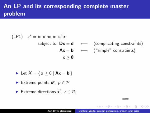
LP-relaxation

(LP1)z∗ = min 2x1 + 3x2 + x3 + 4x4 [cTx]

s.t. 3x1 + 2x2 + 3x3 + 2x4 = 5 [Dx = d]x1 + x2 + x3 + x4 = 2 [x ∈ X ]

0 ≤ x1 , x2 , x3 , x4≤ 1 [x ∈ X ]

◮ X = conv

1100

,

1010

,

1001

,

0110

,

0101

,

0011

= conv {x1, . . . , x6}

=

x ∈ R

4

∣∣∣∣∣∣x =

6∑

p=1

λp xp;

6∑

p=1

λp = 1;λp ≥ 0, p = 1, . . . , 6


The complete master problem and the initial

columns

(LP2)

z∗ = min 5λ1 + 3λ2 + 6λ3 + 4λ4 + 7λ5 + 5λ6

s.t. 5λ1 + 6λ2 + 5λ3 + 5λ4 + 4λ5 + 5λ6 = 5λ1 + λ2 + λ3 + λ4 + λ5 + λ6 = 1

λ1, λ2, λ3, λ4, λ5, λ6≥ 0

◮ Initial columns: λ1, λ2, λ3

(LP2-R) (DLP2-R)

z∗ ≤ min 5λ1 + 3λ2 + 6λ3

s.t. 5λ1 + 6λ2 + 5λ3 = 5λ1 + λ2 + λ3 = 1

λ1, λ2, λ3≥ 0

z∗ ≤ max 5π + q

s.t. 5π + q≤ 56π + q≤ 35π + q≤ 6

◮ Solution: λ = (1, 0, 0)T, π = −2, q = 15


Reduced costs computation

minx∈X

{(c−DTπ)Tx− q

}= min

p=1,...,6

{(c−DTπ)Txp − q

}

= minp=1,...,6

{[(2, 3, 1, 4) − (3, 2, 3, 2) · (−2)] xp − 15

}

= min {0, 0, 1,−1, 0, 0} = −1 < 0

◮ New extreme point in (LP1): x4 = (0, 1, 1, 0)T

◮ New column in (LP2-R):

cTx4

Dx4

1

=

451


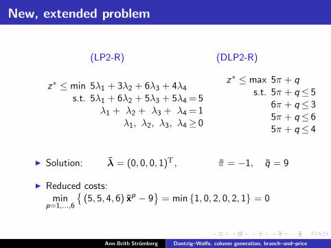
New, extended problem

(LP2-R) (DLP2-R)

z∗ ≤ min 5λ1 + 3λ2 + 6λ3 + 4λ4

s.t. 5λ1 + 6λ2 + 5λ3 + 5λ4 = 5λ1 + λ2 + λ3 + λ4 = 1

λ1, λ2, λ3, λ4≥ 0

z∗ ≤ max 5π + q

s.t. 5π + q≤ 56π + q≤ 35π + q≤ 65π + q≤ 4

◮ Solution: λ = (0, 0, 0, 1)T , π = −1, q = 9

◮ Reduced costs:min

p=1,...,6

{(5, 5, 4, 6) xp − 9

}= min {1, 0, 2, 0, 2, 1} = 0


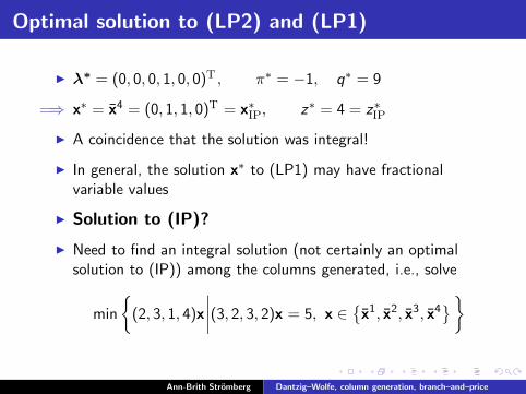
Optimal solution to (LP2) and (LP1)

◮ λ∗ = (0, 0, 0, 1, 0, 0)T , π∗ = −1, q∗ = 9

=⇒ x∗ = x4 = (0, 1, 1, 0)T = x∗IP

, z∗ = 4 = z∗IP

◮ A coincidence that the solution was integral!

◮ In general, the solution x∗ to (LP1) may have fractionalvariable values

◮ Solution to (IP)?

◮ Need to find an integral solution (not certainly an optimalsolution to (IP)) among the columns generated, i.e., solve

min

{(2, 3, 1, 4)x

∣∣∣∣(3, 2, 3, 2)x = 5, x ∈{x1, x2, x3, x4

}}


Another numerical example of Dantzig-Wolfe

decomposition and column generation

min x1 − 3x2 (0)st −x1 + 2x2 ≤ 6 (1) ←− (complicating)

x1 + x2 ≤ 5 (2)x1 , x2 ≥ 0 (3)

x1

x2

5

5

(1)

(2)X

x1

x2

5

5

X

X ={x ∈ R

2+

∣∣ x1 + x2 ≤ 5}

= conv{(0, 0)T, (0, 5)T, (5, 0)T

}


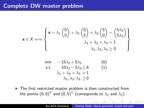
Complete DW master problem

x ∈ X ⇐⇒

x = λ1

(00

)+ λ2

(05

)+ λ3

(50

)=

(5λ3

5λ2

)

λ1 + λ2 + λ3 = 1

λ1, λ2, λ3 ≥ 0

min − 15λ2 + 5λ3 (0)s.t. 10λ2− 5λ3≤ 6 (1)

λ1 + λ2 + λ3 =1λ1, λ2, λ3 ≥ 0

◮ The first restricted master problem is then constructed fromthe points (0, 0)T and (0, 5)T (corresponds to λ1 and λ2)


Iteration 1

◮

min − 15λ2 (0)s.t. 10λ2≤ 6 (1)

λ1 + λ2 = 1λ1, λ2 ≥ 0

∣∣∣∣Solution: λ = (2

5 , 35)T

Dual solution: π = −32 , q = 0

◮ Smallest reduced cost:

minx∈X

[(cT − πD)x− q

]= min

x∈X

([(1,−3) − (− 3

2)(−1, 2)]x− 0

)

= min {− 12x1 | x1 + x2 ≤ 5; x ≥ 02} = − 5

2< 0 =⇒ x =

(50

)

◮ New column:

cTx = (1,−3)(5, 0)T = 5Dx = (−1, 2)(5, 0)T = −5

}=⇒

(5

−51

)


Iteration 2

min −15λ2 + 5λ3

s.t. 10λ2 − 5λ3≤ 6λ1 + λ2 + λ3 = 1

λ1, λ2, λ3≥ 0

∣∣∣∣∣∣∣∣

Solution: λ = (0, 1115 , 4

15)T

Dual solution: π = −43 , q = −5

3

◮ Smallest reduced cost:

minx∈X

[(cT − πD)x− q

]= min

x∈X

([(1,−3)− (− 4

3)(−1, 2)]x− (− 5

3))

= min {− 13x1−

13x2 + 5

3| x1 + x2 ≤ 5; x ≥ 02} = 0

◮ Optimal solution: λ∗ =

(0,

11

15,

4

15

)T

=⇒ x∗ = (5λ3, 5λ2)T = (4

3 , 113 )T; z∗ = 4

3 − 3 · 113 = −92

3


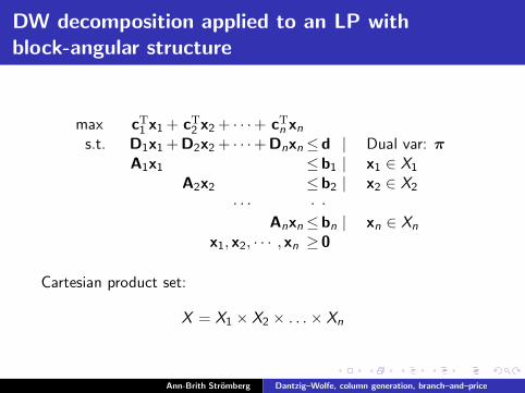
DW decomposition applied to an LP with

block-angular structure

max cT1 x1 + cT

2 x2 + · · ·+ cTn xn

s.t. D1x1 +D2x2 + · · ·+Dnxn≤d | Dual var: π

A1x1 ≤b1 | x1 ∈ X1

A2x2 ≤b2 | x2 ∈ X2

· · · · ·Anxn≤bn | xn ∈ Xn

x1, x2, · · · , xn ≥ 0

Cartesian product set:

X = X1 × X2 × . . .× Xn


DW decomposition as decentralized planning

◮ The main office (master problem) sets prizes (π) for thecommon resources (complicating constraints)

◮ The departments (subproblems) suggest (production) plans(i.e., columns) (Dj x

pj ) based on given prices

◮ The main office “mixes” the suggested plans (columns)optimally; sets new prices

◮ The procedure is repeated

Subproblem 1

Master problem

Subproblem 2 Subproblem n

pricesplan

prices

planplan prices


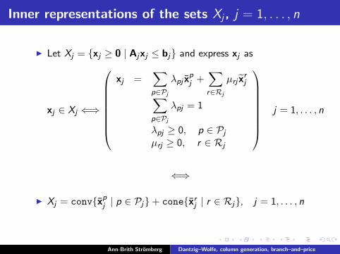
Inner representations of the sets Xj , j = 1, . . . , n

◮ Let Xj = {xj ≥ 0 | Ajxj ≤ bj} and express xj as

xj ∈ Xj ⇐⇒

xj =∑

p∈Pj

λpj xpj +

∑

r∈Rj

µrj xrj

∑

p∈Pj

λpj = 1

λpj ≥ 0, p ∈ Pj

µrj ≥ 0, r ∈ Rj

j = 1, . . . , n

⇐⇒

◮ Xj = conv{xpj | p ∈ Pj}+ cone{xr

j | r ∈ Rj}, j = 1, . . . , n


The complete master problem

max(λ,µ)

n∑

j=1

( ∑

p∈Pj

λpj(cTxp

j ) +∑

r∈Rj

µrj(cTxr

j )

)

s.t.

n∑

j=1

( ∑

p∈Pj

λpj(Dxpj ) +

∑

r∈Rj

µrj(Dxrj )

)≤ d

∑

p∈Pj

λpj = 1, j = 1, . . . , n

λpj ≥ 0, p ∈ Pj , j = 1, . . . , n

µrj ≥ 0, r ∈ Rj , j = 1, . . . , n

◮ The number of constraints in the master problem equals“the number of constraints in Dx = d” + n

◮ The restricted master problem is formulated analogously asbefore (with Pj ⊆ Pj and Rj ⊆ Rj , j = 1, . . . , n)


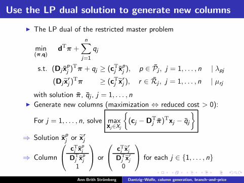
Use the LP dual solution to generate new columns

◮ The LP dual of the restricted master problem

min(π,q)

dTπ +

n∑

j=1

qj

s.t. (Dj xpj )

Tπ + qj ≥ (cT

j xpj ), p ∈ Pj , j = 1, . . . , n | λpj

(Dj xrj )

Tπ ≥ (cT

j xrj ), r ∈ Rj , j = 1, . . . , n | µrj

with solution π, qj , j = 1, . . . , n◮ Generate new columns (maximization ⇔ reduced cost > 0):

For j = 1, . . . , n, solve maxxj∈Xj

{(cj −DT

j π)Txj − qj

}

⇒ Solution xpj or xr

j

⇒ Column

cT

j xpj

DT

j xpj

1

or

cT

j xrj

DT

j xrj

0

for each j ∈ {1, . . . , n}


Find feasible solutions (right-hand side allocation)

◮ Let λpj , p ∈ Pj , and µrj , r ∈ Rj , j = 1, . . . , n, be a feasibleand (almost) optimal solution to the restricted master problem

◮ It then holds thatn∑

j=1

Dj

( ∑

p∈P

λpj xpj +

∑

r∈R

µrj xrj

︸︷︷︸∈Xj

)≤ d

◮ Therefore, a good feasible x-solution is given by the solutionto the program

maximize cTj xj

subject to Djxj ≤∑

p∈P

λpj (Dj xpj ) +

∑

r∈R

µrj(Dj xrj )

xj ∈ Xj

for j = 1, . . . , n


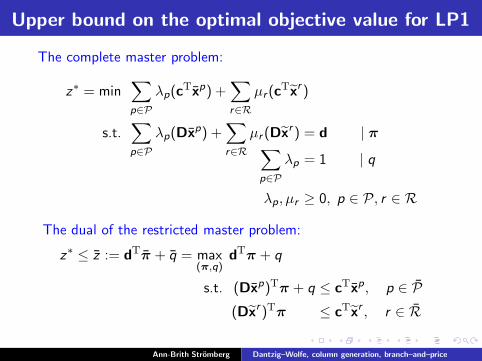
Upper bound on the optimal objective value for LP1

The complete master problem:

z∗ = min∑

p∈P

λp(cTxp) +

∑

r∈R

µr (cTxr )

s.t.∑

p∈P

λp(Dxp) +∑

r∈R

µr (Dxr ) = d | π∑

p∈P

λp = 1 | q

λp, µr ≥ 0, p ∈ P, r ∈ R

The dual of the restricted master problem:

z∗ ≤ z := dTπ + q = max

(π,q)dT

π + q

s.t. (Dxp)Tπ + q ≤ cTxp, p ∈ P

(Dxr )Tπ ≤ cTxr, r ∈ R


Lower bound on the optimal objective value for LP1

◮ Let λ∗p, p ∈ P, and µ∗

r , r ∈ R, be optimal in the completemaster problem

◮ Let (π, q) be an optimal dual solution for the restrictedmaster problem, with columns corresponding to P and R

◮ Multiply the right-hand side elements of the primal (i.e., dand 1) by π and q, respectively

=⇒

0 ≥ z∗−z =z∗−dTπ−1 · q

=∑

p∈P

λ∗p

[cTxp−(Dxp)Tπ−q

]+

∑

r∈R

µ∗r

[cTxr−(Dxr )Tπ

]

≥ minp∈P

[cTxp−(Dxp)Tπ−q

]+

∑

r∈R

µ∗r min

s∈R

[cTxs−(Dxs)Tπ

]


Lower bound on the optimal objective value for LP1

◮ If the subproblem has an unbounded solution no optimisticestimate can be computed in this iteration

◮ Otherwise it holds thatmins∈R

[cTxs − (Dxs)Tπ

]≥ 0

=⇒

z ≥ z∗ ≥ z + minp∈P

[(c−DT

π)Txp − q]

= z + minx∈X

(c−DTπ)Tx− q

=: z


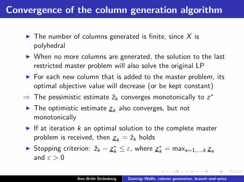
Convergence of the column generation algorithm

◮ The number of columns generated is finite, since X ispolyhedral

◮ When no more columns are generated, the solution to the lastrestricted master problem will also solve the original LP

◮ For each new column that is added to the master problem, itsoptimal objective value will decrease (or be kept constant)

⇒ The pessimistic estimate zk converges monotonically to z∗

◮ The optimistic estimate zk also converges, but notmonotonically

◮ If at iteration k an optimal solution to the complete masterproblem is received, then zk = zk holds

◮ Stopping criterion: zk − z∗k ≤ ε, where z∗k = maxs=1,...,k z s

and ε > 0


Branch–and–price for linear 0/1 problems

(IP)

z∗IP = min cTx

s.t. Dx = d

x ∈ X = {x ∈ Bn | Ax=b}={xp | p ∈ P}

◮ Inner representation (and convexification):

conv X =

x =

∑

p∈P

λpxp

∣∣∣∣∣∣

∑

p∈P

λp = 1; λp ≥ 0, p ∈ P

◮ Let cp = cTxp and dp = Dxp, p ∈ P.


Stronger formulation—Master problem

(CP)

z∗IP = z∗CP = min∑

p∈P

cpλp

s.t.∑

p∈P

dpλp = d

∑

p∈P

λp = 1

λp ∈ {0, 1}, p ∈ P

◮ A continuous relaxation ((CPcont), to λp ≥ 0) of (CP) givesthe same lower bound as the Lagrangian dual with respect tothe constraints Dx = d (z∗LP ≤ zcont

CP ≤ z∗CP)

◮ The continuous relaxation (LP) of (IP) is never better thanany Lagrangian dual bound.


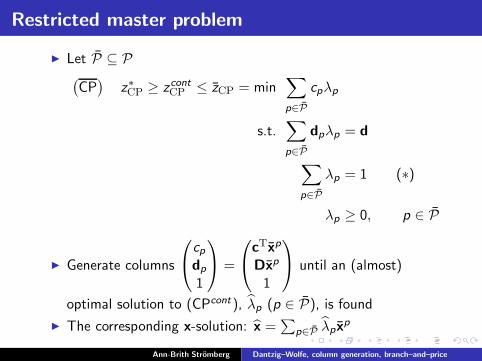
Restricted master problem

◮ Let P ⊆ P(CP

)z∗CP ≥ zcont

CP ≤ zCP = min∑

p∈P

cpλp

s.t.∑

p∈P

dpλp = d

∑

p∈P

λp = 1 (∗)

λp ≥ 0, p ∈ P

◮ Generate columns

cp

dp

1

=

cTxp

Dxp

1

until an (almost)

optimal solution to (CPcont), λp (p ∈ P), is found

◮ The corresponding x-solution: x =∑

p∈P λpxp


Branching over variable xj with 0 < xj < 1

xj = 0 or xj = 1

m m

xj =∑

p∈P

λp xpj = 0 xj =

∑

p∈P

λp xpj = 1

⇓ ⇓

delete col’s∑

p∈P:xpj=1

λp = 0∑

p∈P:xpj=1

λp = 1 replaces (∗)

m m

replaces (∗)∑

p∈P:xpj=0

λp = 1∑

p∈P:xpj=0

λp = 0 delete col’s


Generate columns in B&B nodes

CPk

CPk0 CPk1

xj = 0 xj = 1

zCPk0 ≥ zCPk zCPk1 ≥ zCPk

zCP ≤ zIP

◮ In each node (CP, CP0, CP1, ...): Generate columns until(almost) optimal (all reduced costs ≥ 0) or verified infeasible

◮ If x∗CPkℓ... feasible =⇒ z∗CPkℓ... ≥ z∗IP =⇒ Cut off the branch(k, ℓ, . . . )

=⇒ Cut branches (r , s, . . . ) with z∗CPrs... ≥ z∗CPkℓ...


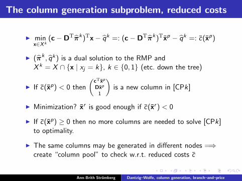
The column generation subproblem, reduced costs

◮ minx∈X k

(c−DTπ

k)Tx− qk =: (c−DTπ

k)Txp − qk =: c(xp)

◮ (πk , qk) is a dual solution to the RMP andX k = X ∩ {x | xj = k}, k ∈ {0, 1} (etc. down the tree)

◮ If c(xp) < 0 then

(cTxp

Dxp

1

)is a new column in [CPk]

◮ Minimization? xr is good enough if c(xr ) < 0

◮ If c(xp) ≥ 0 then no more columns are needed to solve [CPk]to optimality.

◮ The same columns may be generated in different nodes =⇒create “column pool” to check w.r.t. reduced costs c


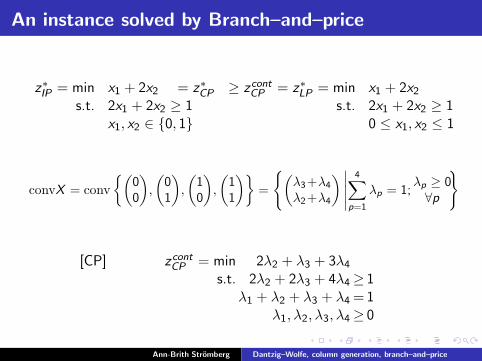
An instance solved by Branch–and–price

z∗IP = min x1 + 2x2 = z∗CP

s.t. 2x1 + 2x2 ≥ 1x1, x2 ∈ {0, 1}

≥ zcontCP = z∗LP = min x1 + 2x2

s.t. 2x1 + 2x2 ≥ 10 ≤ x1, x2 ≤ 1

convX = conv

{(00

),

(01

),

(10

),

(11

)}=

{(λ3+λ4

λ2+λ4

) ∣∣∣∣∣

4∑

p=1

λp = 1;λp ≥ 0∀p

}

[CP] zcontCP = min 2λ2 + λ3 + 3λ4

s.t. 2λ2 + 2λ3 + 4λ4≥ 1λ1 + λ2 + λ3 + λ4 = 1

λ1, λ2, λ3, λ4≥ 0


Initial columns: λ1 and λ3

Choose e.g.,

(00

)and

(10

), that is, the variables λ1 and λ3

zcontCP ≤ min λ3

s.t. 2λ3≥ 1λ1 + λ3 =1

λ1, λ3≥ 0

= max π + q

s.t. q≤ 02π + q≤ 1

π≥ 0

Solution: (λ1, λ3) = (12 , 1

2) =⇒ x = (12 , 0)T, π = 1

2 , q = 0Reduced costs: minx∈[0,1]2 {(0, 1)x} = 0 =⇒ Optimum for CP!

Fix variable values: x1 = 0 or x1 = 1

⇓ ⇓

λ3 = 0 λ1 = 0


Branching, left (CP0): λ3 = 0

min 0s.t. 0≥ 1

λ1 = 1λ1≥ 0

=⇒

infeasible⇓

addcolumn

=⇒

zCP0 ≤ min 2λ2

s.t. 2λ2≥ 1λ1 + λ2 = 1

λ1, λ2≥ 0

= max π + q

s.t. q≤ 02π + q≤ 2

π≥ 0

Solution: (λ1, λ2) = (12 , 1

2 )=⇒ x = (0, 1

2 )T

π = 1, q = 0

Reduced costs: minx∈[0,1]2 {(−1, 0)x − 0} = −1 < 0

=⇒ New column! (λ3 or λ4, but λ3 ≡ 0) =⇒ Choose λ4


zCP0 ≤ min 2λ2 + 3λ4

s.t. 2λ2 + 4λ4≥ 1λ1 + λ2 + λ4 = 1

λ1, λ2, λ4≥ 0

= max π + q

s.t. q≤ 02π + q≤ 24π + q≤ 3

π≥ 0

◮ Solution: (λ1, λ3, λ4) = (34 , 0, 1

4) =⇒ x = (14 , 1

4 )T, π = 34 ,

q = 0

◮ Reduced costs: minx∈[0,1]2 {(−12 , 1

2)x} = −12 =⇒

◮ Generate new column: λ3, but λ3 ≡ 0 =⇒ Optimum for CP0


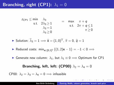
Branching, right (CP1): λ1 = 0

zCP1 ≤ min λ3

s.t. 2λ3≥ 1λ3 = 1λ3≥ 0

= max π + q

s.t. 2π + q≤ 1π≥ 0

◮ Solution: λ3 = 1 =⇒ x = (1, 0)T, π = 0, q = 1

◮ Reduced costs: minx∈[0,1]2 {(1, 2)x − 1} = −1 < 0 =⇒

◮ Generate new column: λ1, but λ1 ≡ 0 =⇒ Optimum for CP1

Branching, left, left: (CP00) λ2 = λ4 = 0

CP00: λ2 = λ3 = λ4 = 0 =⇒ infeasible


Branching, left, right: (CP01) λ1 = 0

CP01: λ1 = λ3 = 0

zCP01 ≤ min 2λ2 + 3λ4

s.t. 2λ2 + 4λ4≥ 1λ2 + λ4 = 1

λ2, λ4≥ 0

= max π + q

s.t. 2π + q≤ 24π + q≤ 3

π≥ 0

◮ Solution: (λ2, λ4) = (1, 0)T =⇒ x = (0, 1)T, π = 0, q = 2

◮ Reduced costs: minx∈[0,1]2 {(1, 2)x − 2} = −2 < 0

=⇒ Generate new column: λ1, but λ1 ≡ 0

=⇒ Generate new column: λ3, but λ3 ≡ 0

=⇒ Optimum for CP01


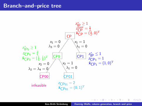
Branch–and–price tree

CP

CP0 CP1

CP00 CP01

x1 = 0 x1 = 1

x2 = 0 x2 = 1

λ3 = 0

λ1 = 0

λ1 = 0

λ2 = λ4 = 0

zCP0 = 34

zCP1 = 1

zCP01 = 2

zcont

CP = 12

z∗IP ≥ 1

z∗IP0≥ 1

z∗IP ≤ 1

xCP = ( 12 , 0)T

xCP0 = ( 14 , 1

4 )T

xCP1 = (1, 0)T

xCP01 = (0, 1)Tinfeasible


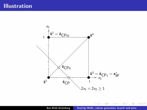
Illustration

1

1

x1

x2

x1

x2 = xCP01

x3 = xCP1 = x∗IP

x4

xCP

xCP0

2x1 + 2x2 ≥ 1


TMA521/MMA510 Optimization, project course Lecture … · TMA521/MMA510 Optimization, project...

Documents

Transcript of TMA521/MMA510 Optimization, project course Lecture … · TMA521/MMA510 Optimization, project...