Cut Generation for Optimization Problems with Multivariate...
29
Cut Generation for Optimization Problems with Multivariate Risk Constraints Simge K¨ u¸ c¨ ukyavuz Department of Integrated Systems Engineering, The Ohio State University, [email protected] Nilay Noyan 1 Manufacturing Systems/Industrial Engineering Program, Sabancı University, Turkey, [email protected] September 15, 2015 Abstract: We consider a class of stochastic optimization problems that features benchmarking preference relations among random vectors representing multiple random performance measures (criteria) of interest. Given a benchmark random performance vector, preference relations are incorporated into the model as constraints, which require the decision-based random vector to be preferred to the benchmark according to a relation based on multivariate conditional value-at-risk (CVaR) or second-order stochastic dominance (SSD). We develop alternative mixed-integer programming formulations and solution methods for cut generation problems arising in optimization under such multivariate risk constraints. The cut generation problems for CVaR- and SSD-based models involve the epigraphs of two distinct piecewise linear concave functions, which we refer to as reverse concave sets. We give the complete linear description of the linearization polytopes of these two non-convex substructures. We present computational results that show the effectiveness of our proposed models and methods. Keywords: stochastic programming; multivariate risk-aversion; conditional value-at-risk; stochastic dominance; cut generation; convex hull; reverse concave set 1. Introduction In many decision making problems, such as those arising in relief network design, home- land security budget allocation, and financial management, there are multiple random performance measures of interest. In such problems, comparing the potential decisions requires specifying preference relations among random vectors, where each dimension of a vector corresponds to a performance measure (or decision criterion). Moreover, it is often crucial to take into account decision makers’ risk preferences. Incorporating stochastic multivariate preference relations into optimization models is a fairly recent research area. The existing models feature benchmarking preference relations as constraints, requiring the decision-based random vectors to be preferred (according to the specified preference rules) to some benchmark random vectors. The literature mainly focuses on multivariate risk-averse preference relations based on SSD or CVaR. The SSD relation has received significant attention due to its correspondence with risk-averse preferences (Hadar and Russell, 1969). In this regard, the majority of existing studies on optimization models with mul- tivariate risk constraints extend the univariate SSD rule to the multivariate case. In this line of research, scalar-based preferences are extended to vector-valued random variables by considering a family of linear scalarization functions and requiring that all scalarized versions of the random vectors conform to the spec- ified univariate preference relation. Scalarization coefficients can be interpreted as weights representing the subjective importance of each decision criterion. Thus, the scalarization approach is closely related to the weighted sum method, which is widely used in multicriteria decision making (see, e.g., Ehrgott, 2005). In such decision-making situations, enforcing a preference relation over a family of scalarization vectors allows the rep- resentation of a wider range of views and differing opinions of multiple experts (for motivating discussions see, e.g., Hu and Mehrotra, 2012). Dentcheva and Ruszczy´ nski (2009) consider linear scalarization with all non- negative coefficients (this set can be equivalently truncated to a unit simplex), and provide a theoretical back- ground for the multivariate SSD-constrained problems. On the other hand, Homem-de-Mello and Mehrotra (2009) and Hu et al. (2012) allow arbitrary polyhedral and convex scalarization sets, respectively. 1
Transcript of Cut Generation for Optimization Problems with Multivariate...
Cut Generation for Optimization Problems with Multivariate Risk Constraints
Simge KucukyavuzDepartment of Integrated Systems Engineering, The Ohio State University, [email protected]
Nilay Noyan1
Manufacturing Systems/Industrial Engineering Program, Sabancı University, Turkey, [email protected]
September 15, 2015
Abstract: We consider a class of stochastic optimization problems that features benchmarking preference relations
among random vectors representing multiple random performance measures (criteria) of interest. Given a benchmark
random performance vector, preference relations are incorporated into the model as constraints, which require the
decision-based random vector to be preferred to the benchmark according to a relation based on multivariate conditional
value-at-risk (CVaR) or second-order stochastic dominance (SSD). We develop alternative mixed-integer programming
formulations and solution methods for cut generation problems arising in optimization under such multivariate risk
constraints. The cut generation problems for CVaR- and SSD-based models involve the epigraphs of two distinct
piecewise linear concave functions, which we refer to as reverse concave sets. We give the complete linear description
of the linearization polytopes of these two non-convex substructures. We present computational results that show the
effectiveness of our proposed models and methods.
Keywords: stochastic programming; multivariate risk-aversion; conditional value-at-risk; stochastic dominance; cut
generation; convex hull; reverse concave set
1. Introduction In many decision making problems, such as those arising in relief network design, home-
land security budget allocation, and financial management, there are multiple random performance measures
of interest. In such problems, comparing the potential decisions requires specifying preference relations among
random vectors, where each dimension of a vector corresponds to a performance measure (or decision criterion).
Moreover, it is often crucial to take into account decision makers’ risk preferences. Incorporating stochastic
multivariate preference relations into optimization models is a fairly recent research area. The existing models
feature benchmarking preference relations as constraints, requiring the decision-based random vectors to be
preferred (according to the specified preference rules) to some benchmark random vectors. The literature
mainly focuses on multivariate risk-averse preference relations based on SSD or CVaR.
The SSD relation has received significant attention due to its correspondence with risk-averse preferences
(Hadar and Russell, 1969). In this regard, the majority of existing studies on optimization models with mul-
tivariate risk constraints extend the univariate SSD rule to the multivariate case. In this line of research,
scalar-based preferences are extended to vector-valued random variables by considering a family of linear
scalarization functions and requiring that all scalarized versions of the random vectors conform to the spec-
ified univariate preference relation. Scalarization coefficients can be interpreted as weights representing the
subjective importance of each decision criterion. Thus, the scalarization approach is closely related to the
weighted sum method, which is widely used in multicriteria decision making (see, e.g., Ehrgott, 2005). In such
decision-making situations, enforcing a preference relation over a family of scalarization vectors allows the rep-
resentation of a wider range of views and differing opinions of multiple experts (for motivating discussions see,
e.g., Hu and Mehrotra, 2012). Dentcheva and Ruszczynski (2009) consider linear scalarization with all non-
negative coefficients (this set can be equivalently truncated to a unit simplex), and provide a theoretical back-
ground for the multivariate SSD-constrained problems. On the other hand, Homem-de-Mello and Mehrotra
(2009) and Hu et al. (2012) allow arbitrary polyhedral and convex scalarization sets, respectively.
1
Kucukyavuz and Noyan: Cut Generation for Multivariate Risk Constraints 2
Optimization models with univariate SSD constraints can be formulated as linear programs with a po-
tentially large number of scenario-dependent variables and constraints (see, e.g., Dentcheva and Ruszczynski,
2006; Noyan et al., 2008; Luedtke, 2008). While efficient cut generation methods can be employed to solve such
large-scale linear programs (Rudolf and Ruszczynski, 2008; Dentcheva and Ruszczynski, 2010; Fabian et al.,
2011), enforcing these constraints for infinitely many scalarization vectors causes additional challenges. For
finite probability spaces, Homem-de-Mello and Mehrotra (2009) show that infinitely many risk constraints (as-
sociated with polyhedral scalarization sets) reduce to finitely (typically exponentially) many scalar-based risk
constraints for the SSD case, naturally leading to a finitely convergent cut generation algorithm. However, such
an algorithm is computationally demanding as it requires the iterative solution of non-convex (difference of
convex functions) cut generation subproblems. The authors formulate the cut generation problem as a binary
mixed-integer program (MIP) by linearizing the piecewise linear shortfall terms, and develop a branch-and-cut
algorithm. They also propose concavity and convexity inequalities, and a big-M improvement method within
the branch-and-cut tree to strengthen the MIP. However, it appears that for the practical applications, the
authors directly solve the MIP formulation of the cut generation problem (Hu et al., 2011; 2012). In another
line of work, Dentcheva and Wolfhagen (2015) use methods from difference of convex (DC) programming to
perform cut generation for the multivariate SSD-constrained problem. The authors also provide a finite rep-
resentation of the multivariate SSD relation if the decisions are taken in a finite dimensional space, even if the
probability space is not finite.
A few studies (Armbruster and Luedtke, 2015; Haskell et al., 2013) consider the multivariate SSD relation
based on multidimensional utility functions instead of using scalarization functions. The resulting models
enforce stricter dominance relations (than those based on the scalarization approach) but they can be formu-
lated as linear programs, and hence, are computationally more tractable. On the other hand, the scalarization
approach allows us to use univariate SSD constraints, which are less conservative than the multivariate version,
and also offers the flexibility to control the degree of conservatism by varying the scalarization sets. However,
the scalarization-based multivariate SSD relation can still be overly conservative in practice and leads to in-
feasible formulations. As an alternative, Noyan and Rudolf (2013) propose the use of constraints based on
coherent risk measures, which provide sufficient flexibility to lead to feasible problem formulations while still
being able to capture a broad range of risk preferences. In particular, they focus on the widely applied risk
measure CVaR, and replace the multivariate SSD relation by a collection of multivariate CVaR constraints at
various confidence levels. This is a very natural relaxation due to the well-known fact that the univariate SSD
relation is equivalent to a continuum of CVaR inequalities (Dentcheva and Ruszczynski, 2006); we note that a
similar idea also led to a cutting plane algorithm for the optimization models with univariate SSD constraints
(Dentcheva et al., 2010). Noyan and Rudolf (2013) define the multivariate CVaR constraints based on the
polyhedral scalarization sets; as a result, their modeling approach strikes a good balance between tractability
and flexibility. They show that, similar to the SSD-constrained counterpart, it is sufficient to consider finitely
many scalarization vectors, and propose a finitely convergent cut generation algorithm. The corresponding cut
generation problem has the DC programming structure, as in the SSD case, with similar MIP reformulations
involving big-M type constraints. In addition, the authors utilize alternative optimization representations
of CVaR to develop MIP formulations for the cut generation problem for the polyhedral CVaR-constrained
problem.
Despite the existing algorithmic developments, solving the MIP formulations of the cut generation problems
Kucukyavuz and Noyan: Cut Generation for Multivariate Risk Constraints 3
can increasingly become a computational bottleneck as the number of scenarios increases. According to the
results presented in Hu et al. (2011) and Noyan and Rudolf (2013), the cut generation generally takes no less
than 90% to 95% of the total time spent. The DC functions encountered in the cut generation problems have
polyhedral structure that can be exploited to devise enhanced and easy-to-implement models. In line with these
discussions, this paper contributes to the literature by providing more effective and easy-to-implement methods
to solve the cut generation problems arising in optimization under multivariate polyhedral SSD and CVaR
constraints. For SSD-constrained problems, the cut generation problems naturally decompose by scenarios,
and the main difficulty is due to the weakness of the MIP formulation involving big-M type constraints. A
similar difficulty arises in CVaR-constrained problems. However, in this case, an additional challenge stems
from the combinatorial structure required to identify the α-quantile of the decision-based random variables.
Therefore, this study is mainly dedicated to developing computationally efficient methods for the multivariate
CVaR-constrained models. However, we also describe how our results can be applied in the SSD case. As
in the previous studies, we focus on finite probability spaces, and our approaches can naturally be used in a
framework based on sample average approximation.
In the next section, we present the general forms of the optimization models featuring the multivariate
polyhedral risk preferences as constraints. In Section 3, we study the cut generation problem arising in CVaR-
constrained models. We give a new MIP formulation, and several classes of valid inequalities that improve
this formulation. In addition, we propose variable fixing methods that are highly effective in certain classes
of problems. The cut generation problem involves the epigraph of a piecewise linear concave function, which
we refer to as a reverse concave set. We give the complete linear description of this non-convex substructure.
In Section 4, we give analogous results for SSD-constrained models. We emphasize that the reverse concave
sets featured in CVaR and SSD cut generation problems are fundamental sets that may appear in other
problems. In Section 5, we present our computational experiments on two data sets: a previously studied
budget allocation problem and a set of randomly generated test instances. Our results show that the proposed
methods lead to more effective cut generation-based algorithms to solve the multivariate risk-constrained
optimization models. We conclude the paper in Section 6.
2. Optimization with multivariate risk constraints In this section, we present the general forms of
the optimization models featuring multivariate CVaR and SSD constraints based on polyhedral scalarization.
Before proceeding, we need to make a note of some conventions used throughout the paper. Larger values of
random variables, as well as larger values of risk measures, are considered to be preferable. In this context,
risk measures are often referred to as acceptability functionals, since higher values indicate less risky random
outcomes. The set of the first n positive integers is denoted by [n] = 1, . . . , n, while the positive part of a
number x ∈ R is denoted by [x]+ = maxx, 0. Throughout this paper, we assume that all random variables
are defined on some finite probability spaces, and simplify our exposition accordingly when possible.
We consider a decision making problem where the multiple random performance measures associated with
the decision vector z are represented by the random outcome vector G(z). Let (Ω, 2Ω,P) be a finite probability
space with Ω = ω1, . . . , ωn and P(ωi) = pi. The set of feasible decisions is denoted by Z and the random
outcomes are determined according to the mapping G : Z ×Ω → R
d. Let f : Z → R be a continuous objective
function and C ⊂ Rd+ be a polytope of scalarization vectors. Considering the interpretation of the scalarization
vectors and the fact that larger outcomes are preferred, we naturally assume that C ⊆ c ∈ Rd+ :
∑
i∈[d] ci =
Kucukyavuz and Noyan: Cut Generation for Multivariate Risk Constraints 4
1. Given the benchmark (reference) random outcome vector Y and the confidence level α ∈ (0, 1], the
optimization problems involving the multivariate polyhedral CVaR and SSD constraints take, respectively,
the following forms:
(G−MCVaR) max f(z)
s.t. CVaRα(c⊤G(z)) ≥ CVaRα(c
⊤Y), ∀ c ∈ C, (1)
z ∈ Z.
(G−MSSD) max f(z)
s.t. c⊤G(z) (2)
c⊤Y, ∀ c ∈ C, (2)
z ∈ Z,
where X <(2) Y denotes that the univariate random variable X dominates Y in the second order. While Y
is allowed to be defined on a probability space different from Ω, it is often constructed from a benchmark
decision z ∈ Z, i.e., Y = G(z). For ease of exposition, we present the formulations with a single multivariate
risk constraint. However, we can also consider multiple benchmarks, multiple confidence levels, and varying
scalarization sets.
According to the results on finite representations of the scalarization polyhedra, it is sufficient to consider
finitely many scalarization vectors in (1) and (2). However, these vectors correspond to the vertices of some
higher dimensional polyhedra, and therefore, there are still potentially exponentially many scalarization-based
risk constraints. A natural approach is to solve some relaxations of the above problems obtained by replacing
the set C with a finite subset (can be even empty). This subset is augmented by adding the scalarization
vectors generated in an iterative fashion. In this spirit, at each iteration of such a cut generation algorithm,
given a current decision vector, we attempt to find a scalarization vector for which the corresponding risk
constraint (of the form (1) or (2)) is violated. The corresponding cut generation problem is the main focus of
our study.
3. Cut Generation for Optimization with Multivariate CVaR Constraints In this section, we
first briefly describe the cut generation problem arising in optimization problems of the form (G−MCVaR).
Then we proceed to discuss the existing mathematical programming formulations of this cut generation prob-
lem, which constitute a basis for our new developments. The rest of the section is dedicated to the proposed,
computationally more effective formulations and methods.
Consider an iteration of the cut generation-based algorithm (proposed in Noyan and Rudolf (2013)), and
let X = G(z∗) be the random outcome vector associated with the decision vector z∗ obtained by solving the
current relaxation of (G−MCVaR) . The aim is to either find a vector c ∈ C for which the corresponding
univariate CVaR constraint (1) is violated or to show that such a vector does not exist. In this regard, we
solve the cut generation problem at confidence level α ∈ (0, 1] of the general form
(CutGen CVaR) minc∈C
CVaRα(c⊤X)− CVaRα(c
⊤Y).
Observe that (CutGen CVaR) involves the minimization of the difference of two concave functions, because
CVaRα(X), given by (Rockafellar and Uryasev, 2000)
CVaRα(X) = max
η −1
αE ([η −X ]+) : η ∈ R
, (3)
Kucukyavuz and Noyan: Cut Generation for Multivariate Risk Constraints 5
is a concave function of a scalar-based random variable X . It is well known that the maximum in definition
(3) is attained at the α-quantile, also known as the value-at-risk at confidence level α denoted by VaRα(X).
If the optimal objective value of (CutGen CVaR) is non-negative, it follows that z∗ is an optimal solution of
(G−MCVaR) . Otherwise, there exists an optimal solution c∗ ∈ C for which the corresponding constraint
CVaRα(c∗⊤X) ≥ CVaRα(c
∗⊤Y) is violated by the current solution.
Note that we can easily calculate the realizations of the random outcomeX = G(z∗) given the decision vector
z∗. In the rest of the paper, we focus on solving the cut generation problems given two d-dimensional random
vectors X and Y with realizations x1, . . . ,xn and y1, . . . ,ym, respectively. Let p1, . . . , pn and q1, . . . , qm
denote the corresponding probabilities.
3.1 Existing mathematical programming formulations In this section, we present one of the
existing mathematical programming formulations of (CutGen CVaR). The second nonlinear term
(−CVaRα(c⊤Y)) in (CutGen CVaR) can be expressed with linear inequalities and continuous variables
because it involves the maximization of a piecewise linear concave function (see (3)). What makes it difficult
to solve (CutGen CVaR) is the minimization of the first concave term (CVaRα(c⊤X)). Using two alterna-
tive optimization representations of CVaR, Noyan and Rudolf (2013) first formulate (CutGen CVaR) as a
(generally nonconvex) quadratic program. Then instead of dealing with the quadratic problem, the authors
propose MIP formulations which are considered to be potentially more tractable.
Note that for finite probability spaces VaRα(c⊤X) = c⊤xk for at least one k ∈ [n], implying
CVaRα(c⊤X) = VaRα(c
⊤X)−1
α
∑
i∈[n]
pi[VaRα(c⊤X)− c⊤xi]+ (4)
= maxk∈[n]
c⊤xk −1
α
∑
i∈[n]
pi[c⊤xk − c⊤xi]+
. (5)
This key observation leads to the following formulation of (CutGen CVaR) (Noyan and Rudolf, 2013):
(MIP CVaR) min µ− η +1
α
∑
l∈[m]
qlwl
s.t. wl ≥ η − c⊤yl, ∀ l ∈ [m], (6)
c ∈ C, w ∈ Rm+ , (7)
µ ≥ c⊤xk −1
α
∑
i∈[n]
pivik, ∀ k ∈ [n], (8)
vik − δik = c⊤xk − c⊤xi, ∀ i ∈ [n], k ∈ [n], (9)
vik ≤ Mikβik, ∀ i ∈ [n], k ∈ [n], (10)
δik ≤ Mik(1− βik), ∀ i ∈ [n], k ∈ [n], (11)
βik ∈ 0, 1, ∀ i ∈ [n], k ∈ [n], (12)
v ∈ Rn×n+ , δ ∈ Rn×n
+ . (13)
Here, the continuous variables η and w together with the linear inequalities (6) are used to express
CVaRα(c⊤Y) according to (3). On the other hand, µ represents CVaRα(c
⊤X) according to the relation
Kucukyavuz and Noyan: Cut Generation for Multivariate Risk Constraints 6
(5), which can be incorporated into the model using the following non-convex constraint
µ ≥ c⊤xk −1
α
∑
i∈[n]
pi[c⊤xk − c⊤xi]+, ∀k ∈ [n].
This non-convex constraint corresponds to the epigraph of a piecewise linear concave function, and the variables
vik and δik are introduced to linearize the shortfall terms [c⊤xk − c⊤xi]+. In addition, Mik and Mik are
sufficiently large constants (big-M coefficients) to make constraints (10) and (11) redundant whenever the
right-hand side is positive. Due to constraints (10)-(13) only one of the variables vik and δik is positive. Then,
constraint (9) ensures that vik = [c⊤xk − c⊤xi]+ for all pairs of i and k. A similar linearization is used for
the SSD case described in Section 4.
Remark 3.1 [Big-M Coefficients] It is well-known that the choice of the big-M coefficients is crucial in ob-
taining stronger MIP formulations. In (MIP CVaR) , we can set
Mik = maxmaxc∈C
c⊤xk − c⊤xi, 0 and Mik = Mki = maxmaxc∈C
c⊤xi − c⊤xk, 0.
These parameters can easily be obtained by solving very simple LPs. Furthermore, in practical applications,
the dimension of the decision vector c and the number of vertices of the polytope C would be small; e.g., in
the homeland security problem in our computational study d = 4. Suppose that the vertices of the polytope C
are known and given as c1, . . . , cN. Then, Mik = maxmaxj∈[N ]
c⊤j (xk − xi), 0.
In the special case when all the outcomes of X are equally likely, Noyan and Rudolf (2013) propose an
alternate MIP formulation which involves only O(n) binary variables instead of O(n2). We refer to the
existing paper for the complete formulation of this special MIP, which is referred to as (MIP Special) in
our study. In the next section, we develop new formulations and methods based on integer programming
approaches. We only focus on the general probability case; it turns out that even these general formulations
perform better than (MIP Special) as we show in Section 5.
3.2 New developments In this section, we first propose several simple improvements to the existing
MIP formulations. Then, we introduce a MIP formulation based on a new representation of VaR. We propose
valid inequalities that strengthen the resulting MIPs. We also give the complete linear description of the
linearization polytope of a non-convex substructure appearing in the new formulation.
3.2.1 Computational enhancements We first present valid inequalities based on the bounds for
CVaRα(c⊤X), and then describe two approaches to reduce the number of variables and constraints of
(MIP CVaR).
Bounds on CVaRα(c⊤X). Suppose that we have a lower bound Lµ and an upper bound Uµ for CVaRα(c
⊤X).
Then, (MIP CVaR) can be strengthened using the following valid inequalities:
Lµ ≤ µ ≤ Uµ. (14)
For example, consider two discrete random variables Xmin and Xmax with realizations minc∈Cc⊤xi, i ∈ [n],
and maxc∈Cc⊤xi, i ∈ [n], respectively. The random variable Xmin is no larger than c⊤X with probability
one for any c ∈ C. Similarly, Xmax is no smaller than c⊤X with probability one for any c ∈ C. Therefore,
we can set Lµ and Uµ as CVaRα(Xmin) and CVaRα(Xmax), respectively. Note that the calculation of the
realizations of Xmin and Xmax requires solving n small (d-dimensional) LPs.
Kucukyavuz and Noyan: Cut Generation for Multivariate Risk Constraints 7
Variable reduction using symmetry. We observe the symmetric relation between the δ and v variables (δik = vki
for all pairs of i ∈ [n] and k ∈ [n]), and substitute vki for δik to obtain a more compact formulation. In
this regard, we only need to define βik for i, k ∈ [n] such that i < k, and write constraints (9)-(11) for
i, k ∈ [n] : i < k. Furthermore, we substitute Mki for Mik, and let vkk = 0 in (8). We refer to the resulting
simplified MIP as (SMIP CVaR); the number of binary variables and constraints (9)-(11) associated with
the shortfall terms is reduced by half. Furthermore, the linearization polytope defined by (9)-(13) can be
strengthened using valid inequalities. In Section 4.2, we study the linearization polytope corresponding to
[c⊤xk − c⊤xi]+ for a given pair i, k ∈ [n]. This substructure also arises in the cut generation problems with
multivariate SSD constraints.
Preprocessing. Let K be a set of scenarios for which c⊤xk cannot be equal to VaRα(c⊤X) for any c ∈ C.
Preprocessing methods can be used to identify the set K, which would allow us to enforce constraint (8) for a
reduced set of scenarios k ∈ K := [n]\K. This would also result in reduced number of variables and constraints
(9)-(13) that are used to represent the shortfall terms. In particular, we need to define the variables vik only
for all k ∈ K, i ∈ [n] and for i ∈ K, k ∈ K. In addition, we define variables βik and constraints (9)-(11) for
i, k ∈ K, i < k and for k ∈ K, i ∈ K (note that due to the elimination of some of the v variables, the symmetry
argument does not hold for the latter condition, so we do not have the restriction that i < k unless i, k ∈ K).
We refer to the resulting more compact MIP, which also involves (14), as (RSMIP CVaR).
Next, we elaborate on how to identify K that yields a reduced set of scenarios K. Recall that we focus
on the left tail of the probability distributions; for example, under equal probabilities, VaRb/n(c⊤X) is the
bth smallest realization of c⊤X where b is a small integer. Thus, c⊤xk values which definitely take relatively
larger values cannot correspond to VaRb/n(c⊤X). In line with these discussions, we use the next proposition
to identify the set K = [n] \K.
Proposition 3.1 Suppose that the parameters Mki are calculated as described in Remark 3.1. For a scenario
index k ∈ [n], let Lk = i ∈ [n] \ k : Mki = 0 and Hk = i ∈ [n] \ k : Mik = 0. If∑
i∈Lk
pi ≥ α then
c⊤xk = VaRα(c⊤X) cannot hold for any c ∈ C, implying k ∈ K. Moreover, i ∈ K for all i ∈ Hk.
Proof. Note that for any k ∈ [n] and i ∈ Lk, Mki = 0 implies that c⊤xi ≤ c⊤xk for all c ∈ C. Thus, the
first claim immediately follows from the following VaR definition: Let c⊤x(1) ≤ c⊤x(2) ≤ · · · ≤ c⊤x(n) denote
an ordering of the realizations of c⊤X for a given c. Then, for a given confidence level α ∈ (0, 1],
VaRα(c⊤X) = c⊤x(k), where k = min
j ∈ [n] :∑
i∈[j]
p(i) ≥ α
. (15)
Similarly, the second claim holds because Lk ⊆ Li for all i ∈ Hk.
Note that if for some k ∈ [n], we have non-empty sets Lk or Hk, we can employ variable fixing by letting
βik = 1, βki = 0 for i ∈ Lk and βik = 0, βki = 1 for i ∈ Hk. Another method can utilize the bounds on
VaRα(c⊤X) while identifying the set K. Suppose that we have a lower bound L and an upper bound U for
VaRα(c⊤X). If max
c∈Cc⊤xk < L or min
c∈Cc⊤xk > U , then k /∈ K. Similar to the case of CVaR, we can calculate
the bounds L and U using the random variables Xmin and Xmax: L = VaRα(Xmin) and U = VaRα(Xmax).
In our numerical study, we have observed that the above methods can significantly impact the computational
performance (see Section 5).
Kucukyavuz and Noyan: Cut Generation for Multivariate Risk Constraints 8
3.2.2 An alternative model based on a new representation of VaR When the realizations are
based on a decision, we cannot know their ordering in advance. While the structure of the objective function
makes it easy to express VaR in the context of VaR or CVaR maximization, in our cut generation problem
we need a new representation of VaR. Recall that we can use the classical definition of CVaR in the second
CVaR term appearing in the objective function of (CutGen CVaR), but for the first CVaR term we need
alternative representations of CVaR to develop new computationally more efficient solution methods. The
main challenge is to express CVaRα(c⊤X), which depends on VaRα(c
⊤X). The next theorem provides a set
of inequalities to calculate VaRα(c⊤X) when c is a decision vector. Before proceeding, we first introduce
some big-M coefficients. Throughout the paper, we use the notation, M , to emphasize that the associated
parameter is used in a big-M type variable upper bounding (VUB) constraint (see, e.g., Mik defined in Remark
3.1 as the maximum possible value of vik = [c⊤(xk − xi)]+ over all c ∈ C, used in the VUB constraint (10)).
Let Mi∗ = maxk∈[n] Mik, be the maximum possible value of [c⊤(xk − xi)]+ taken over all k ∈ [n] for a given
i ∈ [n]. Similarly, let M∗i = maxk∈[n] Mki for i ∈ [n]. Finally, let Mℓ = maxcℓ : c ∈ C for ℓ ∈ [d] be the
maximum possible value of cℓ (note that Mℓ ≤ 1 because C is a subset of the unit simplex).
Theorem 3.1 Suppose that X is a random vector with realizations x1, . . . ,xn and corresponding probabilities
pi, i ∈ [n]. For a given confidence level α and any decision vector c ∈ C, the equality z = VaRα(c⊤X) holds
if and only if there exists a vector (z,β, ζ,u) satisfying the following system:
z ≤ c⊤xi + βiMi∗, i ∈ [n], (16)
z ≥ c⊤xi − (1− βi)M∗i, i ∈ [n], (17)∑
i∈[n]
piβi ≥ α, (18)
∑
i∈[n]
piβi −∑
i∈[n]
piui ≤ α− ǫ, (19)
z =∑
i∈[n]
ζ⊤i xi, (20)
ζiℓ ≤ Mℓui, i ∈ [n], ℓ ∈ [d], (21)∑
i∈[n]
ζiℓ = cℓ, ℓ ∈ [d], (22)
∑
i∈[n]
ui = 1, (23)
ui ≤ βi, i ∈ [n], (24)
β ∈ 0, 1n, ζ ∈ Rn×d+ , u ∈ 0, 1n. (25)
In constraint (19), ǫ is a very small constant to ensure that the left-hand side is strictly smaller than α.
Proof. Suppose that z = VaRα(c⊤X) for a decision vector c ∈ C. Let π be a permutation describing a
non-decreasing ordering of the realizations of the random vector c⊤X, i.e., c⊤xπ(1) ≤ · · · ≤ c⊤xπ(n). Defining
k∗ = min
k ∈ [n] :∑
i∈[k]
pπ(i) ≥ α
and K∗ = π(1), . . . , π(k∗), (26)
and using (15) we have z = c⊤xπ(k∗). Then, a feasible solution of (16)-(25) can be obtained as follows:
βi =
1 i ∈ K∗
0 otherwise, ui =
1 i = k∗
0 otherwise, ζiℓ =
cℓ i = k∗
0 otherwise.
Kucukyavuz and Noyan: Cut Generation for Multivariate Risk Constraints 9
For the reverse implication, let us consider a feasible solution (z,β, ζ,u) of (16)-(25) and let K = i ∈
[n] : βi = 1. To prove our claim, it is sufficient to show that there exists a permutation π where K = K∗
and z = c⊤xπ(k∗) = c⊤xk for a scenario index k ∈ argmaxi∈Kc⊤xi (K∗ and k∗ are defined as in (26)).
We first focus on the intermediate set of linear inequalities (16)-(19), (23)-(24), and the quadratic equality
z =∑
i∈[n]
uic⊤xi. (27)
By the definition of K and inequalities (16)-(17) we have z ≤ c⊤xi, i ∈ [n] \ K, and z ≥ c⊤xi, i ∈ K. Since
βi = 0 for all i ∈ [n] \ K, (24) ensures that ui = 0 for all i ∈ [n] \ K. Then, (23) and (24) guarantee that
z =∑
i∈K
uic⊤xi = c⊤xk for a scenario index k such that c⊤xk = maxi∈Kc⊤xi. Thus, ui = 1 for i = k,
and 0, otherwise. Then, from (18) and (19), P(c⊤X ≤ z) =∑
i∈K
pi ≥ α and∑
i∈K\k
pi < α. It follows that,
according to the definition in (15), VaRα(c⊤X) = c⊤xk = z.
Since c is a decision vector, equality (27) involves quadratic terms of the form uicℓ. First observe that
uicℓ = cℓ, ℓ ∈ [d], for exactly one scenario index i, implying∑
i∈[n] uicℓ = cℓ, ℓ ∈ [d], at any feasible solution
satisfying (16)-(19), (23)-(25), and (27). Therefore, it is easy to show that we can linearize the uicℓ terms by
replacing them with the new decision variables ζiℓ ∈ R+ in (27) to obtain (20), and enforcing the additional
constraints (21)-(22). This completes our proof.
Corollary 3.1 The cut generation problem (CutGen CVaR) is equivalent to the following optimization
problem, referred to as (NewMIP CVaR) :
min z −1
α
∑
i∈[n]
pivi − η +1
α
∑
l∈[m]
qlwl (28)
s.t. (6)− (7), (16)− (25),
vi − δi = z − c⊤xi, i ∈ [n], (29)
vi ≤ Mi∗βi, i ∈ [n], (30)
δi ≤ M∗i(1− βi), i ∈ [n], (31)
v ∈ Rn+, δ ∈ Rn
+, (32)
L ≤ z ≤ U. (33)
Proof. We represent CVaRα(c⊤Y) in (CutGen CVaR) using the classical formulation (3). On the other
hand, we express CVaRα(c⊤X) using the formula (4), i.e., CVaRα(c
⊤X) = z − 1α
∑
i∈[n]
pi[z − c⊤xi]+, where
z = VaRα(c⊤X), and ensure the exact calculation of z for any c ∈ C by enforcing (16)-(25), from Theorem
3.1. Then, by simple manipulation and linearizing the terms [z − c⊤xi]+ =: vi using (29)-(32), we obtain the
desired formulation.
Note that there are O(n) binary variables in (NewMIP CVaR) compared to O(n2) binary variables in
(RSMIP CVaR). We next describe valid inequalities, which we refer to as ordering inequalities, to strengthen
the formulation (NewMIP CVaR).
Proposition 3.2 Suppose that the parameters Mki are calculated as described in Remark 3.1. For a scenario
index k ∈ [n], let Lk = i ∈ [n] \ k : Mki = 0 and Hk = i ∈ [n] \ k : Mik = 0. Then the following sets of
Kucukyavuz and Noyan: Cut Generation for Multivariate Risk Constraints 10
inequalities are valid for (NewMIP CVaR):
βk ≤ βi, k ∈ [n], i ∈ Lk, (34)
or equivalently,
βi ≤ βk, k ∈ [n], i ∈ Hk. (35)
Proof. If i ∈ Lk, then Mki = maxc∈C [c⊤(xi − xk)]+ = 0. In other words, c⊤xk ≥ c⊤xi for all c ∈ C.
Now if z > c⊤xk for some c ∈ C, then βk = 1. Because c⊤xk ≥ c⊤xi, we also have βi = 1. On the other
hand, if z < c⊤xi for some c ∈ C, then βi = 0. Because z < c⊤xi ≤ c⊤xk, we also have βk = 0. Thus,
inequality (34) is valid. The validity proof of inequality (35) follows similarly.
Introducing inequalities (34) or (35) to (NewMIP CVaR) provides us with a stronger formulation. When
the number of such inequalities is considered to be large, we may opt to introduce them only for a selected
set of scenarios. For example, we fix the values of a subset of βi variables using preprocessing methods when
possible, and introduce the ordering inequalities for those that cannot be fixed. The trivial variable fixing sets
βi = 0 or βi = 1 for all i ∈ [n] such that Mi∗ = 0 or M∗i = 0, respectively. In addition, we propose a more
elaborate variable fixing, which relies on Proposition 3.1 to identify the scenarios for which the corresponding
realizations are too large to be equal to VaRα(c⊤X). Suppose we show that k is among such scenarios, i.e.,
k /∈ K. Then, at any feasible solution we have βk = 0, and consequently, βi = 0 for all i ∈ Hk. One can also
employ variable fixing by using the bounds on VaRα(c⊤X). In particular, let βi = 1 if maxc∈C c⊤xi < L and
let βi = 0 if minc∈C
c⊤xi > U . We note that the proposed ordering inequalities and variable fixing methods can
also be applied to other relevant MIP formulations involving βi decisions. In such MIPs, e.g., (MIP Special),
the set k ∈ [n] : βk = 1 corresponds to the realizations which are less than or equal to VaRα(c⊤X).
3.2.3 Linearization of (z − x⊤c)+ in (CutGen CVaR) Consider the convex function g(z, c) =
[z − x⊤i c]+ := max0, z − x⊤
i c for (z, c) ∈ Rd+1+ and i ∈ [n] such that
∑
j∈[d] cj = 1, which appears in (4)
with z = VaRα(c⊤X). Using formula (4) in (CutGen CVaR) leads to a concave minimization. Therefore,
we study the linearization of the set (referred to as a reverse concave set) corresponding to the epigraph of
−g(z, c), given by (29)-(32) in (NewMIP CVaR). We propose valid inequalities that give a complete linear
description of this linearization set for a given i ∈ [n]. As a result, these valid inequalities can be used to
strengthen the formulation (NewMIP CVaR) (as will be shown in our computational study in Section 5).
Throughout this subsection, we drop the scenario indices and focus on the linearization of one term of
the form [z − x⊤c]+. Due to the translation invariance of CVaR, we assume without loss of generality that
all the realizations of X are non-negative. Therefore, xj ≥ 0, j ∈ [d]. This implies the nonnegativity of
z = VaRα(c⊤X), since c ≥ 0. In addition, to avoid trivial cases, we assume that xj > 0 for some j ∈ [d],
because otherwise, we can let z = v and δ = 0. We are interested in the polytope defined by
v − δ = z −∑
j∈[d]
xjcj , (36)
v ≤ Mvβ, (37)
δ ≤ Mδ(1− β), (38)∑
j∈[d]
cj = 1, (39)
c, v, δ ≥ 0, (40)
Kucukyavuz and Noyan: Cut Generation for Multivariate Risk Constraints 11
β ∈ 0, 1, (41)
0 ≤ z ≤ U . (42)
At this time, we let U = maxs∈[n],k∈[d]xsk, i.e, the largest component of xs over all s ∈ [n], which is a
trivial upper bound on VaRα(c⊤X). Also let Mv = U −mink∈[d]xk be the big-M coefficient for the variable
v = [z−∑
j∈[d] xjcj ]+, and Mδ = maxk∈[d]xk be the big-M coefficient for the variable δ = [∑
j∈[d] xjcj−z]+.
Let Q = (c, v, δ, β, z) : (36)− (42).
First, we characterize the extreme points of conv(Q). Throughout, we let ek denote the d-dimensional unit
vector with 1 in the kth entry and zeroes elsewhere.
Proposition 3.3 The extreme points (c, v, δ, β, z) of conv(Q) are as follows:
QEP1k: (ek, 0, xk, 0, 0) for all k ∈ [d] with xk > 0,
QEP2k: (ek, 0, 0, 0, xk) for all k ∈ [d],
QEP3k: (ek, 0, 0, 1, xk) for all k ∈ [d],
QEP4k: (ek, U − xk, 0, 1, U) for all k ∈ [d] with xk < U .
Proof. First, note that, from the definitions of U , Mv, and Mδ, we have xk ≤ Mδ ≤ U , and 0 ≤
U − xk ≤ Mv for all k ∈ [d]. Hence, points QEP1k–QEP4k are feasible and they cannot be expressed as a
convex combination of any other feasible points of conv(Q). Finally, observe that any other feasible point with
0 < cj < 1 for some j ∈ [d] cannot be an extreme point, because it can be written as a convex combination of
QEP1k–QEP4k.
Note that if xk = 0 for some k ∈ [d], then QEP1k is equivalent to QEP2k. Therefore, we only define
QEP1k for k ∈ [d] with xk > 0. Similarly, if xk = U for some k ∈ [d], then QEP4k is equivalent to QEP3k.
Therefore, we only define QEP4k for k ∈ [d] with xk < U .
Next we give valid inequalities for Q.
Proposition 3.4 For k ∈ [d], the inequality
v ≤∑
j∈[d]
[xk − xj ]+cj + (U − xk)β (43)
is valid for Q. Similarly, for k ∈ [d], the inequality
δ ≤∑
j∈[d]
[xj − xk]+cj + xk(1− β) (44)
is valid for Q.
Proof. First, we prove the validity of inequality (43). If β = 0, then v = 0 from (37). Because c ≥ 0,
inequality (43) holds trivially. If β = 1, then δ = 0 from (38). Thus, for any k ∈ [d],
v − δ = v = z −∑
j∈[d]
xjcj + xk(∑
j∈[d]
cj − 1) = z +∑
j∈[d]
(xk − xj)cj − xk
≤∑
j∈[d]
[xk − xj ]+cj + U − xk =∑
j∈[d]
[xk − xj ]+cj + (U − xk)β,
Kucukyavuz and Noyan: Cut Generation for Multivariate Risk Constraints 12
where the last inequality follows from (42). Thus, inequality (43) is valid.
Next, we prove the validity of inequality (44). If β = 1, then δ = 0 from (38). Because c ≥ 0, inequality
(44) holds trivially. If β = 0, then v = 0 from (38). Thus, for any k ∈ [d],
δ =∑
j∈[d]
xjcj − z ≤∑
j∈[d]
(xj − xk)cj + xk ≤∑
j∈[d]
[xj − xk]+cj + xk(1− β).
Hence, inequality (44) is valid.
Theorem 3.2 conv(Q) is completely described by equalities (36) and (39), and inequalities (40), (43), and
(44).
Proof. Let O(γ, γv, γδ, γβ, γz), denote the index set of extreme point optimal solutions to the problem
minγ⊤c + γvv + γδδ + γββ + γzz : (c, v, δ, β, z) ∈ conv(Q), where (γ, γv, γδ, γβ, γz) ∈ Rd+4 is an arbi-
trary objective vector, not perpendicular to the smallest affine subspace containing conv(Q). In other words,
(γ, γv, γδ, γβ , γz) 6= λ(−x,−1, 1, 0, 1) and (γ, γv, γδ, γβ, γz) 6= λ(1, 0, 0, 0, 0) for λ ∈ R. Therefore, the set of
optimal solutions is not conv(Q) (conv(Q) 6= ∅). We prove the theorem by giving an inequality among (40),
(43), and (44) that is satisfied at equality by (cκ, vκ, δκ, βκ, zκ) for all κ ∈ O(γ, γv, γδ, γβ, γz) for the given
objective vector. Then, since (γ, γv, γδ, γβ , γz) is arbitrary, for every facet of conv(Q), there is an inequality
among (40), (43), and (44) that defines it. Throughout the proof, without loss of generality, we assume that
x1 ≤ x2 ≤ · · · ≤ xd. We consider all possible cases.
Case A. Suppose that γβ ≥ 0. Without loss of generality we can assume that γδ = 0 by adding γδ(v − δ −
z +∑
j∈[d] xjcj) to the objective. From equation (36) the added term is equal to zero, and so this operation
does not change the set of optimal solutions. Furthermore, we can also assume that γj ≥ 0 for all j ∈ [d]
without loss of generality by subtracting γk∗(∑
j∈[d] cj) from the objective, where k∗ := argminγj, j ∈ [d].
From equation (39), the subtracted term is a constant (γk∗), and so this operation does not change the set
of optimal solutions. Therefore, for the case that γβ ≥ 0, we assume that γδ = 0, γj ≥ 0 for all j ∈ [d], and
γk∗ = 0. Under these assumptions, we can express the cost of each extreme point solution (denoted by C(·))
given in Proposition 3.3:
C(QEP1k) = γk for k ∈ [d] with xk > 0,
C(QEP2k) = γk + γzxk for k ∈ [d],
C(QEP3k) = γk + γzxk + γβ for k ∈ [d],
C(QEP4k) = γk + γzU + γβ + γv(U − xk) for k ∈ [d] with xk < U .
Note that QEP1k for k ∈ [d] with xk > 0 are the only extreme points with δ > 0, and QEP4k for k ∈ [d] with
xk < U are the only extreme points with v > 0. We use this observation in the following cases we consider.
(i) γz < 0. In this case, C(QEP2k)< C(QEP1k) for all k ∈ [d] with xk > 0. Therefore, δκ = 0 for all
κ ∈ O(γ, γv, γδ, γβ , γz).
(ii) γz ≥ 0. In this case, C(QEP1k)≤ C(QEP2k)≤ C(QEP3k) for all k ∈ [d]. Note that C(QEP4k)=
C(QEP3k)+(γz + γv)(U − xk), k ∈ [d]. Therefore, if γz + γv > 0, then C(QEP4k)> C(QEP3k)
for all k ∈ [d], and hence extreme points QEP4k, k ∈ [d] are never optimal. As a result, vκ = 0
for all κ ∈ O(γ, γv , γδ, γβ , γz). So we can assume that γz + γv ≤ 0. Because γz ≥ 0, we must
Kucukyavuz and Noyan: Cut Generation for Multivariate Risk Constraints 13
have γv ≤ 0. Let φk := γzU + γβ + γv(U − xk) for k ∈ [d]. Therefore, C(QEP4k) = γk + φk.
Note that φ1 ≤ φ2 ≤ · · · ≤ φd because x1 ≤ x2 ≤ · · · ≤ xd ≤ U and γv ≤ 0 by assumption. If
φ1 > 0, then φk > 0 and so C(QEP4k)> C(QEP1k) for all k ∈ [d]. Therefore, extreme points
QEP4k, k ∈ [d] are never optimal. Hence, vκ = 0 for all κ ∈ O(γ, γv, γδ, γβ, γz). Similarly, if φd < 0,
then φk < 0 for all k ∈ [d]. Therefore, extreme points QEP1k, k ∈ [d] are never optimal. Hence,
δκ = 0 for all κ ∈ O(γ, γv, γδ, γβ, γz). As a result, we can assume that φ1 ≤ 0 and φd ≥ 0. If there
exists j ∈ [d] such that γj > 0 and γj + φj > 0, then C(QEP1k∗)= 0 < C(QEP1j)≤ C(QEP2j)≤
C(QEP3j)< C(QEP4j). Hence, cκj = 0 for all κ ∈ O(γ, γv , γδ, γβ , γz). As a result, we can assume
that either γk = 0 or γk + φk ≤ 0 for all k ∈ [d]. If there exists j ∈ [d] such that γj > 0 and
γj + φj < 0 = C(QEP1k∗), then extreme points QEP1k, k ∈ [d] are never optimal. Hence, δκ = 0
for all κ ∈ O(γ, γv , γδ, γβ, γz). As a result, we can assume that for every k ∈ [d], either γk = 0 or
γk + φk = 0.
(a) If γβ > 0, then the optimal extreme point solutions are QEP1j for all j ∈ [d] such that γj = 0;
QEP2j for all j ∈ [d] such that γj = 0 if γz = 0; andQEP4k for all k ∈ [d] such that γk+φk = 0.
Let k′ := maxj ∈ [d] : φj ≤ 0. Note that φj > 0 for j > k′ by definition, which implies that
γj + φj > 0. Therefore, we must have γj = 0 for j > k′. Then inequality (43) for k′ holds at
equality for all optimal solutions O(γ, γv, γδ, γβ, γz).
(b) If γβ = 0 and γz > 0, then the optimal extreme point solutions are QEP1j for all j ∈ [d] such
that γj = 0 and QEP4k for all k ∈ [d] such that γk + φk = 0. Then inequality (43) for k′ holds
at equality for all optimal solutions O(γ, γv, γδ, γβ, γz).
(c) The only case left to consider is if γβ = γz = 0. In this case, because we assume that γv ≤ 0,
there are two cases to consider. If γv = 0, then φk = 0 for all k ∈ [d] and we must have γk = 0
for all k ∈ [d], which contradicts our initial assumption that (γ, γv, γδ, γβ , γz) 6= λ(1, 0, 0, 0, 0)
for any λ ∈ R. Therefore, we must have γv < 0. In this case, φk < 0 for all k ∈ [d]. Suppose
there exists k∗ ∈ [d] (with γk∗ = 0) such that xk∗ < U . Then, C(QEP4k∗)< 0 = C(QEP1k∗).
Because C(QEP1k∗)≤ C(QEP1j) for all j ∈ [d], extreme points QEP1j , j ∈ [d] are never
optimal. Hence, δκ = 0 for all κ ∈ O(γ, γv, γδ, γβ, γz). The only case left to consider is when
xk = U for all k with γk = 0. In this case, inequality (43) for k∗ holds at equality for all optimal
solutions O(γ, γv, γδ, γβ, γz). This completes the proof of Case A.
Case B. Suppose that γβ < 0. As before, we can assume that γj ≥ 0 for all j ∈ [d], and that γk∗ = 0 for some
k∗ ∈ [d]. Finally, we can assume that γv = 0 by subtracting γv(v − δ − z +∑
j∈[d] xjcj) from the objective.
Under these assumptions, we can express the cost of each extreme point solution (denoted by C(·)) given in
Proposition 3.3:
C(QEP1k) = γk + γδxk for k ∈ [d] with xk > 0,
C(QEP2k) = γk + γzxk for k ∈ [d],
C(QEP3k) = γk + γzxk + γβ for k ∈ [d],
C(QEP4k) = γk + γzU + γβ for k ∈ [d] with xk < U .
Note that due to the assumption that γβ < 0, C(QEP2k)> C(QEP3k) for all k ∈ [d]. So the extreme points
QEP2k, k ∈ [d] are never optimal under these cost assumptions. We use this observation in the following
cases we consider.
Kucukyavuz and Noyan: Cut Generation for Multivariate Risk Constraints 14
(i) γz > 0. In this case, C(QEP4k)> C(QEP3k) for all k ∈ [d]. (Recall that QEP4k exists for some
k ∈ [d] only if U > xk.) So the extreme points QEP4k, k ∈ [d] are never optimal under these cost
assumptions. Hence, vκ = 0 for all κ ∈ O(γ, γv, γδ, γβ, γz).
(ii) γz ≤ 0. If γz ≤ γδ, then C(QEP1k)> C(QEP3k) for all k ∈ [d]. Therefore, extreme points
QEP1k, k ∈ [d] are never optimal. Hence, δκ = 0 for all κ ∈ O(γ, γv , γδ, γβ, γz). As a result, we can
assume that γδ < γz ≤ 0 and C(QEP4k)≤ C(QEP3k) for all k ∈ [d]. Note that because γδ < 0,
0 > γδx1 ≥ γδx2 ≥ · · · ≥ γδxd. In addition, mink∈[d]C(QEP4k) = C(QEP4k∗)= γzU + γβ . If
γδxd > γzU + γβ, then extreme points QEP1k, k ∈ [d] are never optimal. Hence, δκ = 0 for all
κ ∈ O(γ, γv, γδ, γβ , γz). So we can assume that γδxd ≤ γzU + γβ . If γδx1 < γzU + γβ , then extreme
points QEP4k, k ∈ [d] are never optimal. Hence, vκ = 0 for all κ ∈ O(γ, γv, γδ, γβ, γz). So we can
assume that γδx1 ≥ γzU + γβ . Let k := minj ∈ [d] : γδxj ≤ γzU + γβ. If there exists j ≥ k such
that C(QEP1j)= γj + γδxj < γzU + γβ = C(QEP4k∗)≤ C(QEP4k) for all k ∈ [d], then extreme
points QEP4k, k ∈ [d] are never optimal. Hence, vκ = 0 for all κ ∈ O(γ, γv , γδ, γβ, γz). Therefore,
we have γj + γδxj = γzU + γβ for all j ≥ k. Under these assumptions, the optimal solutions are
QEP1j for j ≥ k; QEP4k for k ∈ [d] such that γk = 0; and QEP3k for k ∈ [d] such that γk = 0
if γz = 0. Then inequality (44) for k holds at equality for all optimal solutions O(γ, γv, γδ, γβ, γz).
This completes the proof.
Note that in the definition of the set Q, we used weaker bounds on v, δ and z than are available using the
improvements proposed in Section 3. In particular, we can let z ≤ U , where U is the upper bound on VaR
obtained by using the quantile information (as described in Section 3.2.1); in most cases, U < U . Then, we
simply update inequality (43) as
v ≤∑
j∈[d]
[xk − xj ]+cj + (U − xk)β. (45)
In addition, we can let z ≥ L, using the lower bound information on VaR, and typically L > 0. If this is the
case, then we can define new variables z′ = z − L and δ′ = δ − L, and let M ′z = U − L and M ′
δ = Mδ − L,
and obtain a linearization polytope of the same form as Q in the (c, v, δ′, β, z′) space. The updated inequality
(44) in the original space becomes
δ ≤∑
j∈[d]
[xj − xk]+cj + (xk − L)(1− β). (46)
Therefore, our results hold for L > 0 with this translation of variables.
Finally, from Section 3, we know that v ≤ Mi∗β and δ ≤ M∗i(1−β) for the given scenario i ∈ [n] for which
the linearization polytope is written. Again, in most cases, Mi∗ ≤ Mv and M∗i ≤ Mδ. In this case, we cannot
have ck = 1 and z = L for k such that xk−L > M∗i, because otherwise δ = [∑
j∈[d] cjxj−z]+ = xk−L > M∗i,
which violates the constraint δ ≤ M∗i(1 − β). Hence for all k with xk − L > M∗i, if ck > 0 and z = L, then
we must have cℓ = 1 − ck for some ℓ ∈ [d] with xℓ − L < M∗i. Then, δ = M∗i in such an extreme point
solution. In this case, we can construct an equivalent polyhedron where we let xℓk = M∗i + L for all k ∈ [d]
such that xk − L > M∗i and ℓ ∈ [d] such that xℓ − L < M∗i. Similarly, we cannot have ck = 1 and z = U
for k such that U − xk > Mi∗, because otherwise v = [z −∑
j∈[d] cjxj ]+ = U − xk > Mi·, which violates the
constraint v ≤ Mi·β. If ck > 0 for k with U − xk > Mi∗, then we must have cℓ = 1 − ck for some ℓ ∈ [d]
with U − xℓ < Mi∗. Then v = Mi∗ in such an extreme point solution. In this case, we can construct an

Kucukyavuz and Noyan: Cut Generation for Multivariate Risk Constraints 15
equivalent polyhedron where we let xℓk = U − Mi∗ for all k ∈ [d] such that U − xk > Mi∗ and ℓ ∈ [d] such
that U − xℓ < Mi∗. The resulting polyhedron satisfies the bound assumptions in the definition of Q, and the
non-trivial inequalities that define its convex hull are given by (45) for k ∈ [d] such that U − xk ≤ Mi∗, and
inequality (46) for k ∈ [d] such that xk − L ≤ M∗i. Note that after this update inequalities (45) for k ∈ [d]
such that U − xk = Mi∗ reduces to v ≤ Mi∗β, and inequality (46) for k ∈ [d] such that xk −L = M∗i reduces
to δ ≤ M∗i(1− β). Translating back to the original space of variables and re-introducing the scenario indices
we have the following corollary.
Corollary 3.2 For i ∈ [n], consider the polyhedron Q′i = (c, vi, δi, βi, z) ∈ R
d+4+ : (29)−(31), (33), (39), βi ∈
0, 1. Then conv(Q′i) is completely described by adding inequalities
vi ≤∑
j∈[d]
[xik − xij ]+cj + (U − xik)βi, ∀ k ∈ [d] : U − xik < Mi∗, (47)
δi ≤∑
j∈[d]
[xij − xik]+cj + (xik − L)(1− βi), ∀ k ∈ [d] : xik − L < M∗i (48)
to the original constraints (29)-(31),(33), and (39).
In this section and in Section 4.2, we derive valid inequalities and convex hull descriptions using only the
condition that C is a unit simplex. However, we note that the unit simplex condition applies, without loss of
generality, to all scalarization sets of interest, and therefore, the presented inequalities are valid even if there
are additional constraints on the scalarization vectors, i.e., even if C is a strict subset of the unit simplex.
4. Cut Generation for Optimization with Multivariate SSD Constraints In this section, we
study the cut generation problem arising in optimization problems of the form (G−MSSD) . As in Section
3, we focus on solving the cut generation problems given two d-dimensional random vectors X and Y with
realizations x1, . . . ,xn and y1, . . . ,ym, respectively. Let p1, . . . , pn and q1, . . . , qm denote the corresponding
probabilities, and let C be a polytope of scalarization vectors.
The random vector X is said to dominate Y in polyhedral linear second order with respect to C if and only
if
E([c⊤yl − c⊤X]+) ≤ E([c⊤yl − c⊤Y]+), ∀ l ∈ [m], c ∈ C, or equivalently,
∑
i∈[n]
pi[c⊤yl − c⊤xi]+ ≤
∑
k∈[m]
qk[c⊤yl − c⊤yk]+, ∀ l ∈ [m], c ∈ C. (49)
As discussed in Section 2, Homem-de-Mello and Mehrotra (2009) show that for finite probability spaces it
is sufficient to consider a finite subset of scalarization vectors, obtained as projections of the vertices of m
polyhedra. Specifically, each polyhedron corresponds to a realization of the benchmark random vector Y and
is given by Pl = wk ≥ c⊤yl − c⊤yk, k ∈ [m], c ∈ C, w ∈ Rm+ for l ∈ [m]. Thus, (G−MSSD) can
be reformulated as an optimization problem with exponentially many constraints, and solved using a delayed
constraint generation algorithm (Homem-de-Mello and Mehrotra, 2009). The SSD constraints corresponding
to a subset of the scalarization vectors are initially present in the formulation. Then given a solution to this
intermediate relaxed problem, a cut generation problem is solved to identify whether there is a constraint
violated by the current solution.
Kucukyavuz and Noyan: Cut Generation for Multivariate Risk Constraints 16
Due to the structure of the SSD relation (49), a separate cut generation problem is defined for each
realization of the benchmark random vector. Thus, in contrast to the CVaR-constrained models, the number
of cut generation problems depends on the number of benchmark realizations. The cut generation problem
associated with the lth realization of the benchmark vector Y is given by
(CutGen SSD) minc∈C
∑
k∈[m]
qk[c⊤yl − c⊤yk]+ −
∑
i∈[n]
pi[c⊤yl − c⊤xi]+.
4.1 Existing mathematical programming approaches Note that (CutGen SSD) involves a min-
imization of the difference of convex functions. Dentcheva and Wolfhagen (2015) use methods from
DC programming to solve this problem directly. Similar to the case of univariate SSD constraints
(Dentcheva and Ruszczynski, 2003), we can easily linearize the first type of shortfalls featured in the objective
function:
min
∑
k∈[m]
qkwk −∑
i∈[n]
pi[c⊤yl − c⊤xi]+ : (c,w) ∈ Pl
, (50)
which results in a concave minimization with potentially many local minima. If the optimal objective function
value of (50) is smaller than 0, then there is a scalarization vector for which the SSD condition associated
with the lth realization is violated. Note that it is crucial to solve the cut generation problem exactly for the
correct execution of the solution method for (G−MSSD) . Otherwise, if we obtain a local minimum and the
objective is positive, then we might prematurely stop the algorithm.
The methods based on DC programming and concave minimization may not fully utilize the polyhedral
nature of the objective and the constraints. In addition, DC methods can only guarantee local optimality. The
main challenge in the cut generation problem (50) is to linearize the second type of shortfalls appearing in the
objective function. In this regard, Homem-de-Mello and Mehrotra (2009) introduce additional variables and
constraints, and obtain the following MIP formulation of (CutGen SSD) associated with the lth realization
of the benchmark vector Y:
(MIP SSDl) min∑
k∈[m]
qkwk −∑
i∈[n]
pivi
s.t. wk ≥ c⊤yl − c⊤yk, ∀ k ∈ [m], (51)
w ∈ Rm+ , (52)
vi − δi = c⊤yl − c⊤xi, ∀ i ∈ [n], (53)
vi ≤ Miβi, ∀ i ∈ [n], (54)
δi ≤ Mi(1− βi), ∀ i ∈ [n], (55)
c ∈ C, v ∈ Rn+, δ ∈ Rn
+, β ∈ 0, 1n. (56)
Here we can set Mi = maxmaxc∈C
c⊤yl − c⊤xi, 0 and Mi = −minminc∈C
c⊤yl − c⊤xi, 0. This formulation
guarantees that vi = [c⊤yl − c⊤xi]+ for all i ∈ [n].
The authors also propose concavity and convexity cuts to strengthen the formulation (MIP SSDl). How-
ever, the concavity cuts require the complete enumeration of a set of edge directions (may be exponential),
and solving a system of linear equations based on this enumeration. Hence, this may not be practicable. In
addition, the convexity cuts require the solution of another cut generation LP in higher dimension. Indeed, in
their computational study, Hu et al. (2011) do not utilize these cuts and solve (MIP SSDl) directly. They also
note that this step is the bottleneck taking over 90% of the total solution time, and it needs to be improved.
Kucukyavuz and Noyan: Cut Generation for Multivariate Risk Constraints 17
4.2 New developments We begin by presenting an analogue of Proposition 3.2, which provides valid
ordering inequalities that strengthen the formulation (MIP SSDl). Then, we study the structure of a gen-
eralization of the linearization polytope defined by (53)-(56) for a given l ∈ [m] and i ∈ [n]. We give two
classes of valid inequalities analogous to those in Proposition 3.4 for this polytope. Furthermore, we show
that these inequalities are enough to give the complete linear description when added to the formulation with
C = c ∈ Rd+ :
∑
j∈[d] cj = 1.
Lemma 4.1 The ordering inequalities (34)–(35) are also valid for (MIP SSDl) given lth realization of the
benchmark random vector Y.
This claim immediately follows from the trivial observation that z can be replaced by c⊤yl in (29) (and also
in the proof of Proposition 3.2) for any l ∈ [m]. Next we give a polyhedral study of the set defining the
linearization of the piecewise linear convex shortfall terms.
Linearization of [a⊤c]+ in (CutGen SSD). For a given vector a ∈ Rd, consider the convex function h(c) =
[a⊤c]+ := max0, a⊤c for c ∈ Rd+ such that
∑
j∈[d] cj = 1. This function appears in the cut generation
problems for optimization under multivariate risk given in (50), where a = yl−xi for some l ∈ [m] and i ∈ [n].
An MIP linearizing this term is given in (MIP SSDl). Therefore, we study the linearization of the set (also a
reverse concave set) corresponding to the epigraph of −h(c). (Note that this structure also appears in the cut
generation problem for CVaR (9)–(13), where we let a = xk −xi, for i, k ∈ [n].) We propose valid inequalities
that give a complete linear description of this linearization set for a given i ∈ [n]. As a result, these valid
inequalities can be used to strengthen the formulations involving such linearization terms.
Let D+ = j ∈ [d] : aj ≥ 0 and D− = j ∈ [d] : aj < 0. Due to the nature of the cut generation problems,
we can assume that D+ 6= ∅ and D− 6= ∅ (otherwise, we can fix the corresponding binary variables). Without
loss of generality, we assume that D+ = 1, . . . , d1 with a1 ≤ a2 ≤ · · · ≤ ad1 , and D− = d1 + 1, . . . , d with
−ad1+1 ≤ −ad1+2 ≤ · · · ≤ −ad.
In this subsection, we drop the scenario indices, and study the polytope given by
v − δ =∑
j∈[d]
ajcj , (57)
v ≤ Mvβ, (58)
δ ≤ Mδ(1− β), (59)∑
j∈[d]
cj = 1, (60)
c, v, δ ≥ 0, (61)
β ∈ 0, 1, (62)
where Mv = ad1 is the big-M coefficient associated with the variable v = [∑
j∈[d] ajcj ]+, and Mδ = −ad is the
big-M coefficient associated with the variable δ = [∑
j∈[d] −ajcj ]+.
Let S = (c, v, δ, β) : (57) − (62). First, we characterize the extreme points of conv(S). Recall that ek
denotes the d-dimensional unit vector with 1 in the kth entry and zeroes elsewhere.
Proposition 4.1 The extreme points (c, v, δ, β) of conv(S) are as follows:
Kucukyavuz and Noyan: Cut Generation for Multivariate Risk Constraints 18
EP1k: (ek, ak, 0, 1) for all k ∈ D+,
EP2ℓ: (eℓ, 0,−aℓ, 0) for all ℓ ∈ D−,
EP3k,ℓ: ( −aℓ
ak−aℓek +
ak
ak−aℓeℓ, 0, 0, 1) for all k ∈ D+ and ℓ ∈ D−,
EP4k,ℓ: ( −aℓ
ak−aℓek +
ak
ak−aℓeℓ, 0, 0, 0) for all k ∈ D+ and ℓ ∈ D−.
Proof. First, note that, from the definition of Mv, Mδ, D+ and D−, we have 0 ≤ ak ≤ Mv for all k ∈ D+
and 0 < −aℓ ≤ Mδ for ℓ ∈ D−. Hence, points EP1k and EP2ℓ are feasible and they cannot be expressed as
a convex combination of any other feasible points of conv(S). Finally, observe that any other feasible point
with 0 < ck < 1 for some k ∈ D+, we must have cℓ = 1− ck for some ℓ ∈ D− in any extreme point of conv(S)
such that ckak + cℓaℓ = 0 = v = δ. In this case, we can have either β = 0 or β = 1. As a result, we obtain the
extreme points EP3k,ℓ and EP4k,ℓ. This completes the proof.
Next we give valid inequalities for S.
Proposition 4.2 For k = 1, . . . , d1, the inequality
v ≤d1∑
j=1
[aj − ak]+cj + akβ (63)
is valid for S. Similarly, for k = d1 + 1, . . . , d, the inequality
δ ≤d
∑
j=d1+1
[ak − aj ]+cj − ak(1− β) (64)
is valid for S.
Proof. If β = 0, then v = 0 from (58). Because c ≥ 0, inequality (63) holds trivially. If β = 1, then
δ = 0 from (59). Thus, for any k = 1, . . . , d1,
v − δ = v =∑
j∈[d]
ajcj ≤d1∑
j=1
ajcj =
d1∑
j=1
(aj − ak)cj + ak
d1∑
j=1
cj
≤d1∑
j=1
[aj − ak]+cj + ak =
d1∑
j=1
[aj − ak]+cj + akβ,
where the last inequality follows from (60).
To see the validity of inequality (64), note that equality (57) can be rewritten as δ − v =∑
j∈[d](−aj)cj .
Thus, we obtain an equivalent set where v and δ, and D+ and D− are interchanged.
Remark 4.1 Inequality (58) is a special case of (63) with k = d1, and inequality (59) is a special case of
(64) with k = d.
Remark 4.2 Note that β ≥ 0 is implied by inequality (58), and β ≤ 1 is implied by (59).
Remark 4.3 Consider a related set, T , where constraint (60) is relaxed to∑
j∈[d] cj ≤ 1. This set can be
written in the form of the set S with c ∈ Rd+1, where D = 0, . . . , d, and a0 = 0. In this case, inequality
(63) for k = 0 is given by v ≤∑d1
j=1 ajcj.
Kucukyavuz and Noyan: Cut Generation for Multivariate Risk Constraints 19
Theorem 4.1 conv(S) is completely described by equalities (57) and (60), and inequalities (61), (63), and
(64).
Proof. Let O(γ, γv, γδ, γβ), denote the index set of extreme point optimal solutions to the problem
minγ⊤c + γvv + γδδ + γββ : (c, v, δ, β) ∈ conv(S), where (γ, γv, γδ, γβ) ∈ Rd+3 is an arbitrary objective
vector, not perpendicular to the smallest affine subspace containing conv(S). In other words, (γ, γv, γδ, γβ) 6=
λ(a,−1, 1, 0) and (γ, γv, γδ, γβ) 6= λ(1, 0, 0, 0) for λ ∈ R. Therefore, the set of optimal solutions is not conv(S)
(conv(S) 6= ∅). We prove the theorem by giving an inequality among (61), (63), and (64) that is satisfied at
equality by (cκ, vκ, δκ, βκ) for all κ ∈ O(γ, γv, γδ, γβ) for the given objective vector. Then, since (γ, γv, γδ, γβ)
is arbitrary, for every facet of conv(S), there is an inequality among (61), (63), and (64) that defines it. We
consider all possible cases.
Case A. Suppose that γβ ≥ 0. Without loss of generality we can assume that γδ = 0 by adding γδ(v − δ −∑
j∈[d] ajcj) to the objective. From equation (57) the added term is equal to zero, and so this operation does
not change the set of optimal solutions. Furthermore, we can also assume that γj ≥ 0 for all j ∈ D without loss
of generality by subtracting γmin(∑
j∈[d] cj) from the objective, where γmin := minj∈[d]γj. From equation
(60), the added term is a constant (−γmin), and so this operation does not change the set of optimal solutions.
Note also that after this update γmin = 0. Therefore, for the case that γβ ≥ 0, we assume that γδ = 0 and
γmin = 0. Under these assumptions, we can express the cost of each extreme point solution (denoted by C(·))
given in Proposition 4.1:
C(EP1k) = γk + γvak + γβ for k ∈ D+,
C(EP2ℓ) = γℓ for ℓ ∈ D−,
C(EP3k,ℓ) = γk−aℓ
ak−aℓ+ γℓ
ak
ak−aℓ+ γβ for k ∈ D+ and ℓ ∈ D−,
C(EP4k,ℓ) = γk−aℓ
ak−aℓ+ γℓ
ak
ak−aℓfor k ∈ D+ and ℓ ∈ D−.
Let k∗ ∈ argminγj, j ∈ D+ and ℓ∗ ∈ argminγj , j ∈ D−. Note that minγk∗ , γℓ∗ = γmin = 0. Observe
that C(EP2ℓ)< C(EP4k,ℓ) for k ∈ D+ and ℓ ∈ D− if γℓ < γk. On the other hand, if γℓ > γk, then
C(EP2ℓ)> C(EP4k,ℓ) for k ∈ D+ and ℓ ∈ D−. Also, the only extreme points for which δ > 0 are EP2ℓ for
ℓ ∈ D− with −aℓ > 0, and the only extreme points for which v > 0 are EP1k for k ∈ D+ with ak > 0. We
use these observations in the following cases we consider.
(i) γℓ∗ = 0 < γk∗ . In this case, EP4k,ℓ cannot be an optimal solution for any k ∈ D+ and ℓ ∈ D−.
Furthermore, because of the assumption that γβ ≥ 0, EP3k,ℓ cannot be an optimal solution for any
k ∈ D+ and ℓ ∈ D− either.
(a) If there exists j ∈ D+ such that C(EP1j)=γj + γvaj + γβ > 0 = C(EP2ℓ∗), then cκj = 0 for all
κ ∈ O(γ, γv, γδ, γβ). So we can assume that γk + γvak + γβ ≤ 0 for all k ∈ D+. Now suppose
that γj + γvaj + γβ < 0 for some j ∈ D+. In this case, C(EP1j)< C(EP2ℓ) for all ℓ ∈ D−.
Therefore, δκ = 0 for all κ ∈ O(γ, γv, γδ, γβ). So we can assume that γk + γvak + γβ = 0 for all
k ∈ D+.
(b) If there exists j ∈ D− such that C(EP2j)=γj > 0 = C(EP2ℓ∗), then cκj = 0 for all κ ∈
O(γ, γv, γδ, γβ). So we can assume that γℓ = 0 for all ℓ ∈ D−. In summary, for the case that
γβ ≥ 0 and γℓ∗ = 0 < γk∗ , we have γk + γvak + γβ = 0 for all k ∈ D+ and γℓ = 0 for all ℓ ∈ D−.
Kucukyavuz and Noyan: Cut Generation for Multivariate Risk Constraints 20
In this case, the set O(γ, γv, γδ, γβ) is given by EP1k for all k ∈ D+ and EP2ℓ for all ℓ ∈ D−.
Inequality (63) for k = 1 is tight for all these extreme point optimal solutions. Hence, the proof
is complete for this case.
(ii) γℓ∗ > γk∗ = 0. Recall that, in this case, C(EP4k∗,ℓ)< C(EP2ℓ) for all ℓ ∈ D−. Therefore, δκ = 0 for
all κ ∈ O(γ, γv , γδ, γβ). Hence, the proof is complete for this case.
(iii) γℓ∗ = γk∗ = 0.
(a) If there exists j ∈ D− such that γj > 0, then cκj = 0 for all κ ∈ O(γ, γv, γδ, γβ). So we can
assume that γℓ = 0 for all ℓ ∈ D−.
(b) Suppose that γj + γvaj + γβ < 0 for some j ∈ D+. In this case, EP1j has a strictly better
objective value than EP2ℓ, EP3k,ℓ, and EP4k,ℓ for all k ∈ D+ and ℓ ∈ D−. Therefore, δκ = 0
for all κ ∈ O(γ, γv, γδ, γβ). So we can assume that γk + γvak + γβ ≥ 0 for all k ∈ D+. If there
exists j ∈ D+ such that γj > 0 and γj + γvaj + γβ > 0, then cκj = 0 for all κ ∈ O(γ, γv, γδ, γβ).
So we can assume that at least one of the conditions γk = 0 or γk + γvak + γβ = 0 holds for
all k ∈ D+. Let D+0 = j ∈ D+ : γj = 0 and D+
1 = D+ \ D+0 . Note that k∗ ∈ D+
0 and
γk + γvak + γβ = 0 for all k ∈ D+1 .
(c) Suppose that γk = 0 for all k ∈ D+ (i.e., D+1 = ∅). Recall that we also have γℓ = 0 for all
ℓ ∈ D−, γδ = 0 and γβ ≥ 0. If γβ = 0, then γv cannot equal to 0 (then all solutions are
optimal). Suppose that γβ = 0, then γv > 0 (because we showed that γk + γvak + γβ ≥ 0 for
all k ∈ D+). Then vκ = 0 for all κ ∈ O(γ, γv, γδ, γβ). So we can assume that γβ > 0. If γv ≥ 0,
then EP1k is not optimal for any k ∈ D+. Therefore, vκ = 0 for all κ ∈ O(γ, γv, γδ, γβ). So
we can assume that γv < 0. Because we showed that γk + γvak + γβ ≥ 0 for all k ∈ D+, and
we assume that γk = 0 for all k ∈ D+, we have γβ ≥ −γvad1 . If γvad1 + γβ > 0, then EP1k is
not optimal for any k ∈ D+. Therefore, vκ = 0 for all κ ∈ O(γ, γv, γδ, γβ), and we can assume
that γvad1 + γβ = 0. In this case, inequality (63) for k = d1 holds at equality for the set of all
optimal extreme solutions O(γ, γv, γδ, γβ) (namely, EP1k for k ∈ D+ with ak = ad1 , EP2ℓ and
EP4j,ℓ for all j ∈ D+ and ℓ ∈ D−).
(d) There exists k ∈ D+ such that γk > 0 (i.e., D+1 6= ∅). In this case, for k ∈ D+
1 , γk = −γvak−γβ >
0. Because γβ ≥ 0, we must have γv < 0 and ak > 0 for k ∈ D+1 . In this case, we cannot have
γβ = 0 (unless aj = 0 for all j ∈ D+0 ), because otherwise γj + γvaj + γβ < 0 for j ∈ D+
0 with
aj > 0 violating the condition in part (b) that γk + γvak + γβ ≥ 0 for all k ∈ D+. So γβ > 0
and EP3j,ℓ is not optimal for any j ∈ D+, ℓ ∈ D−. Let k1 = minj ∈ D+1 , then we must have
k ∈ D+1 for all k ∈ D+ with k > k1. In this case, the set of all optimal solutions is given by
EP1k for k ∈ D+1 , EP2ℓ and EP4j,ℓ for all j ∈ D+
0 and ℓ ∈ D−, where the optimal objective
value is zero. Then inequality (63) for k = k1 holds at equality for the set of all optimal extreme
solutions O(γ, γv , γδ, γβ). The last case to consider is that aj = 0 for all j ∈ D+0 and hence
γβ = 0. In this case, inequality (63) for k = k∗ holds at equality for the set of all optimal
extreme solutions O(γ, γv , γδ, γβ) (namely, EP1k for k ∈ D+, EP2ℓ, EP3j,ℓ and EP4j,ℓ for all
j ∈ D+0 and ℓ ∈ D−).
Case B. Suppose that γβ < 0. Without loss of generality we can assume that γv = 0 by subtracting
γv(v − δ −∑
j∈[d] ajcj) from the objective. From equation (57), the subtracted term is equal to zero, and so
Kucukyavuz and Noyan: Cut Generation for Multivariate Risk Constraints 21
this operation does not change the set of optimal solutions. As argued in the proof of the validity of (64),
equality (57) can be rewritten as δ − v =∑
j∈[d](−aj)cj . Thus, we obtain an equivalent set where v and δ,
and D+ and D− are interchanged. Thus, the proof is complete, using the same arguments as in Case A and
inequalities (64).
In line with the above analysis, we introduce aij = (yl −xi)j , D+i = j ∈ [d] : aij ≥ 0 and D−
i = j ∈ [d] :
aij < 0 for all i ∈ [n]. Then, an enhanced MIP formulation of (CutGen SSD) for the lth realization of Y
is obtained by replacing (54)-(55) in (MIP SSDl) with the following constraints:
vi ≤∑
j∈D+i
[aij − aik]+cj + aikβi, ∀ i ∈ [n], k ∈ D+i , (65)
δi ≤∑
j∈D−
i
[aik − aij ]+cj − aik(1− βi), ∀ i ∈ [n], k ∈ D−i . (66)
5. Computational Study The goals of our computational study are two-fold. In the first part, we
demonstrate that the methods developed in Section 3.2 – including variable fixing, bounding, and incorporating
valid inequalities – are effective in solving (CutGen CVaR). In the second part, we perform a similar analysis
for the methods presented in Section 4 for (CutGen SSD).
All the optimization problems are modeled with the AMPL mathematical programming language. All
runs were executed on 4 threads of a Lenovo(R) workstation with two Intel R© Xeon R© 2.30 GHz CE5-2630
CPUs and 64 GB memory running on Microsoft Windows Server 8.1 Pro x64 Edition. All reported times
are elapsed times, and the time limit is set to 5400 seconds. CPLEX 12.2 is invoked with its default set of
options and parameters. If optimality is not proven within the time allotted, we record both the best lower
bound on the optimal objective value (retrieved from CPLEX and denoted by LB) and the best available
objective value (denoted by UB). In cut generation problems, the optimal objective function can take any
value including 0, and so in order to provide more insight, we calculate two types of relative optimality gap:
G1 = |LB−UB |/(|UB |) and G2 = |LB−UB |/(|LB |). It is easy to see that the maximum of G1 and G2 is
an upper bound on the actual relative optimality gap; we do not report G1 when |UB | = 0 or CPLEX yields a
trivial lower bound of −∞.
We would like to remind the reader that during a cut generation-based algorithm, the solution procedure of
the cut generation problem is allowed to terminate early without finding the most violated cut. However, when
such a heuristic procedure cannot find a violated cut, it is still required to prove that the optimal objective
function value is non-negative. Therefore, in our experiments we opt for solving the cut generation problem
to optimality.
5.1 Generation of the problem instances In this section, we describe two sets of data used for our
computational experiments.
5.1.1 Homeland security budget allocation We test the computational effectiveness of our proposed
methods on a homeland security budget allocation (HSBA) problem presented in Hu et al. (2011) for op-
timization under multivariate polyhedral SSD constraints. We follow the related data generation scheme
described in Noyan and Rudolf (2013), where the polyhedral SSD constraints are replaced by the CVaR-based
ones. The main problem is to allocate a fixed budget to ten urban areas in order to prevent, respond to,
Kucukyavuz and Noyan: Cut Generation for Multivariate Risk Constraints 22
and recover from national disasters. The risk share of each area is based on four criteria: property losses,
fatalities, air departures, and average daily bridge traffic. The penalty for allocations under the risk share
is expressed by a budget misallocation function associated with each criterion, and these functions are used
as the multiple random performance measures of interest. In order to be consistent with our convention of
preferring larger values, we construct random outcome vectors of interest from the negative of the budget
misallocation functions associated with four criteria. Two different benchmarks are considered: one based on
average government allocations by the Department of Homeland Security’s Urban Areas Security Initiative,
and one based on suggestions in the RAND report by Willis et al. (2005). The scalarization polytope is of the
form C =
c ∈ R4 : ‖c‖1 = 1, ci ≥ c∗i −θ3
, where c∗ ∈ R4 is a center satisfying ‖c∗‖1 = 1, and θ ∈ [0, 1] is
a constant for which θ3 ≤ min
i∈1,...,4c∗i holds. We consider the “base case” with θ = 0.25 and c∗ = (14 ,
14 ,
14 ,
14 ),
unless otherwise stated. We refer the reader to Hu et al. (2011) and Noyan and Rudolf (2013) for more details
on the data generation.
For this set of instances, Noyan and Rudolf (2013) report computational results with the formulation
(MIP Special) – developed for the multivariate CVaR-constrained problem under the special case of equal
probabilities. For example, for the largest problem instances with 500 scenarios and α = 0.05 (resp., α = 0.01),
on average, two (resp., 1.6) cut generation problems need to be solved taking 14386 (resp., 11507) seconds
(around 99.8% of overall solution time). We note that in the initialization step of the algorithm, four risk con-
straints are additionally generated based on the vertices of C. Similarly, for the multivariate SSD-constrained
problems, Hu et al. (2011) report that for the largest test problems with 300 scenarios, only one cut generation
problem is solved taking 1,318 seconds (96% of overall solution time). Since the cut generation is the main
bottleneck, in our computational study we only focus on solving the cut generation problems. Hence, different
from the existing studies, we also explain how we obtain the realizations of the random vectorX. In accordance
with the existing studies, the risk constraints associated with the vertices of the scalarization polytope C are
initially added to the intermediate relaxed problem. In the base case, the polytope C is a three-dimensional
simplex with the vertices c1, . . . , c4, where the ith element of ci is equal to 0.5, and other elements are 0.5/3.
We solve the master problem once, and use its optimal solution to calculate the realizations of the associated
4-dimensional random vector X. Note that it is clear how to obtain the realizations of the random vector Y,
since the benchmark allocations are given.
5.1.2 Randomly generated data To further analyze the computational performance of the proposed
methods, we consider a different type of problem (inspired by Dentcheva and Wolfhagen, 2015):
maxf(z) : Rz < Y, z ∈ R100+ ,
whereR : Ω 7→ [0, 1]d×100 is a random matrix and the relation< represents a stochastic multivariate preference
relation. In our setup, the relation < represents <CCVaRα
and <C(2) for the multivariate polyhedral CVaR and
SSD relation, respectively. We assume that the benchmark vector Y takes the form of Rz, where R is also a
d× 100-dimensional random matrix and z ∈ R100+ is a given benchmark decision. The entries of the matrices
R and R are independently generated from the uniform distribution on the interval [0, 1]. Since we directly
focus on solving the associated cut generation problems, we also randomly generated the decision variables z
and z; in particular, they are independently and uniformly generated from the interval [100, 500]. This data
generation scheme directly provides us with the realizations of two d-dimensional random vectors X = Rz
and Y = Rz.
Kucukyavuz and Noyan: Cut Generation for Multivariate Risk Constraints 23
5.2 Computational performance - cut generation for (G − MCVaR) First, we study the ef-
fectiveness of alternative MIP formulations for (CutGen CVaR). In these experiments, we assume that
each scenario is equally likely, and consider confidence levels of the form α = k/n. For an arbitrary confi-
dence level α, we calculate k as ⌈αn⌉. In Table 1, we present our experiments on the performances of four
alternative formulations: (i) the MIP model – (MIP Special) – developed for the special case of equal prob-
abilities (Noyan and Rudolf, 2013), (ii) the MIP model – (MIP CVaR) – for general probabilities presented
in Noyan and Rudolf (2013), (iii) the more compact model – (SMIP CVaR) – proposed in Section 3.2.1, and
(iv) the new model – (NewMIP CVaR) – proposed in Section 3.2.2. We report the results averaged over
two instances (based on Government and RAND benchmarks) for each combination of α and n. We see that
the new formulation using the VaR representation is highly effective in reducing the solution time for these
instances. Problem instances that are not solvable within the time limit of 5400 seconds with the existing
formulation (MIP CVaR) and its enhancement (SMIP CVaR), is now solvable in six minutes for all in-
stances but one (HSBA data, n = 1000, α = 0.05), which is also solved well within the time limit. We observe
that (MIP CVaR) terminates at the root node for large instances with no integer feasible solution available.
This may be due to the large size of the formulation (quadratic number of binary variables). In contrast,
(NewMIP CVaR) contains a linear number of binary variables. What is also surprising is that even the for-
mulation (MIP Special), which uses more information due to the equal probability assumption, is not able to
solve many of the instances. For the HSBA data set, (MIP Special) has inferior performance when compared
to (SMIP CVaR) for problems with 300 or more scenarios. On the other hand, for the random data set
(described in Section 5.1.2) (MIP Special) performs better than (MIP CVaR) and (SMIP CVaR). How-
ever, it still cannot solve larger instances with 500 or more scenarios. In contrast, (NewMIP CVaR) solves
these problems within a few minutes. We would also like to note that the total time spent on preprocessing
for (NewMIP CVaR) (calculation of the parameters L,U,Mik,Mi∗,M∗i, Hk), which is not included in the
times reported, is negligible. Therefore, we can conclude that (NewMIP CVaR) is a better formulation than
the existing formulations (MIP Special), (MIP CVaR) and its enhancement (SMIP CVaR).
Next we study the effectiveness of various classes of valid inequalities and preprocessing strategies described
in Sections 3.2.2 and 3.2.3. Note that when we test the performance of a class of inequalities, we add all
inequalities a priori to the formulation, because there are polynomially many of them. We consider two sets of
data as before, one with HSBA data (Table 2), and one with the randomly generated data (Table 3). In Tables
2 and 3, the relative improvements and optimality gaps are given as percentages and all presented results are
averaged over the two instances with different benchmarks. In the first two columns of Table 2, we compare
the performance of (RSMIP CVaR), which is the original formulation enhanced with variable reduction
due to symmetry, variable fixing and bounding, against the new formulation (NewMIP CVaR) without
any enhancements. In the third column of Table 2, we report the performance of (NewMIP CVaR) with
variable fixing and bounding. Finally, in the fourth column, we report the performance of (NewMIP CVaR)
with variable fixing, bounding and ordering inequalities (34). Comparing the first two columns of Table 2, we
see that fixing and bounding the variables are highly effective strategies, and as a result (RSMIP CVaR)
outperforms (NewMIP CVaR). However, it cannot solve the larger instances within the time limit, and
in general stops with a large relative optimality gap. On the other hand, when these strategies are also
applied to (NewMIP CVaR), all test instances are solved within the time limit, as observed from the third
column. The reduction in solution time comparing columns 2 and 3 can be attributed to the large reduction
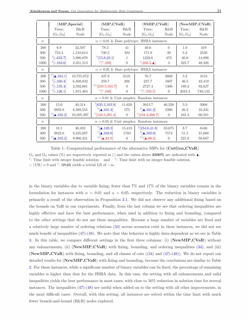
Kucukyavuz and Noyan: Cut Generation for Multivariate Risk Constraints 24
(MIP Special) (MIP CVaR) (SMIP CVaR) (NewMIP CVaR)
Time; B&B Time; B&B Time; B&B Time; B&B
[G1,G2] Node [G1,G2] Node [G1,G2] Node [G1,G2] Node
n α = 0.01 & Base polytope: HSBA instances
200 6.8 22,507 78.2 41 40.6 0 1.0 419
300 752.4 1,510,614 746.5 494 171.9 39 5.2 2556
500 †[-,632.7] 5,980,878 †[15.8,23.1] 1 1232.6 473 40.0 14,806
1000 †[-,163.6] 2,351,513 ⋄[∗,100] 0 ⋄[105.5,N] 3 325.7 48,326
n α = 0.05 & Base polytope: HSBA instances
200 †[N,164.1] 10,755,872 437.8 6121 76.7 2668 5.2 4154
300 †[-,160.4] 6,408,832 259.7 266 237.7 1607 46.5 42,419
500 †[-,135.4] 2,592,061 †⋄[233.5,555.7] 0 2727.4 1306 189.2 92,627
1000 †[-,126.1] 1,915,464 ⋄[∗,100] 0 ⋄[∗,593.5] 0 2034.3 749,132
n α = 0.01 & Unit simplex: Random instances
200 15.0 40,314 †[635.2,103.8] 11,629 3913.7 46,358 5.9 3008
300 3892.8 8,388,555 †[N,101.3] 575 †[N,101.2] 2390 26.2 10,331
500 †[N,102.2] 10,505,307 ⋄[134.5,201.4] 0 ⋄[104.3,208.7] 0 165.3 60,581
n α = 0.05 & Unit simplex: Random instances
200 18.1 40,493 †[N,120.2] 15,419 †[254.6,41.8] 33,675 8.7 6446
300 3822.6 8,235,087 †[N,103.0] 1703 †[N,102.0] 7574 51.5 21,668
500 †[N,102.2] 9,960,451 †⋄[N,83.9] 0 †⋄[N,80.2] 0 221.0 58,687
Table 1: Computational performance of the alternative MIPs for (CutGen CVaR)
G1 and G2 values (%) are respectively reported in [ ] and the values above 3500% are indicated with N.†: Time limit with integer feasible solution and ⋄: Time limit with no integer feasible solution.
-: |UB | = 0 and ∗: CPLEX yields a trivial LB of −∞.
in the binary variables due to variable fixing; fewer than 7% and 17% of the binary variables remain in the
formulation for instances with α = 0.01 and α = 0.05, respectively. The reduction in binary variables is
primarily a result of the observation in Proposition 3.1. We did not observe any additional fixing based on
the bounds on VaR in our experiments. Finally, from the last column we see that ordering inequalities are
highly effective and have the best performance, when used in addition to fixing and bounding, compared
to the other settings that do not use these inequalities. Because a large number of variables are fixed and
a relatively large number of ordering relations (34) across scenarios exist in these instances, we did not see
much benefit of inequalities (47)-(48). We note that this behavior is highly data-dependent as we see in Table
3. In this table, we compare different settings in the first three columns: (i) (NewMIP CVaR) without
any enhancements, (ii) (NewMIP CVaR) with fixing, bounding, and ordering inequalities (34), and (iii)
(NewMIP CVaR) with fixing, bounding, and all classes of cuts ((34) and (47)-(48)). We do not report our
detailed results for (NewMIP CVaR) with fixing and bounding, because the conclusions are similar to Table
2. For these instances, while a significant number of binary variables can be fixed, the percentage of remaining
variables is higher than that for the HSBA data. In this case, the setting with all enhancements and valid
inequalities yields the best performance in most cases, with close to 50% reduction in solution time for several
instances. The inequalities (47)-(48) are useful when added on to the setting with all other improvements, in
the most difficult cases. Overall, with this setting, all instances are solved within the time limit with much
fewer branch-and-bound (B&B) nodes explored.
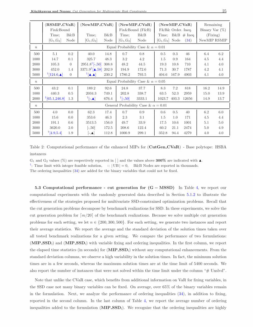
Kucukyavuz and Noyan: Cut Generation for Multivariate Risk Constraints 25
(RSMIP CVaR) (NewMIP CVaR) (NewMIP CVaR) (NewMIP CVaR) Remaining
Fix&Bound Fix&Bound (F&B) F&B& Order. Ineq. Binary Var (%)
Time; B&B Time; B&B Time; B&B Time; B&B # Ineq (Fixing)
[G1,G2] Node [G1,G2] Node [G1,G2] Node [G1,G2] Node (34) NewMIP RSMIP
n Equal Probability Case & α = 0.01
500 5.1 0.2 40.0 14.8 0.7 0.8 0.5 0.3 46 6.4 6.2
1000 14.7 0.1 325.7 48.3 3.2 4.2 1.5 0.9 164 4.5 4.4
2000 105.3 0 2951.8† [-,50] 308.8 48.2 44.5 19.3 10.8 710 4.1 4.0
3000 452.0 1.4 3371.9† [N,58] 202.9 194.9 172.6 71.3 30.7 1787 4.2 4.1
5000 †[124.6,N] 0 †[N,N] 230.2 1780.2 793.5 404.6 167.9 4903 4.1 4.0
n Equal Probability Case & α = 0.05
500 43.2 0.1 189.2 92.6 24.8 37.7 8.3 7.2 818 16.2 14.9
1000 440.3 0.5 2034.3 749.1 202.8 338.7 63.5 52.3 2959 15.0 13.9
2000 †[65.1,246.8] 1.3 †[-,N] 676.4 †[-,50] 3333.1 1023.7 403.3 12656 14.9 13.7
n General Probability Case & α = 0.01
500 4.0 0.0 62.3 17.4 0.7 0.9 0.6 0.5 40 6.2 6.0
1000 15.6 0.0 353.6 46.3 2.3 3.1 1.5 1.0 171 4.5 4.4
2000 191.1 0.6 3513.5 156.0 49.7 33.9 17.5 10.6 1001 5.1 5.0
3000 3620.0 2.0 [-,50] 172.5 208.6 122.4 60.2 21.1 2474 5.0 4.9
5000 †[4.9,5.4] 1.9 [-,N] 112.8 1000.9 299.1 352.8 94.4 4279 4.0 4.0
Table 2: Computational performance of the enhanced MIPs for (CutGen CVaR) - Base polytope: HSBA
instances
G1 and G2 values (%) are respectively reported in [ ] and the values above 300% are indicated with N.†: Time limit with integer feasible solution, -: |UB | = 0, B&B Nodes are reported in thousands.
The ordering inequalities (34) are added for the binary variables that could not be fixed.
5.3 Computational performance - cut generation for (G − MSSD) In Table 4, we report our
computational experiments with the randomly generated data described in Section 5.1.2 to illustrate the
effectiveness of the strategies proposed for multivariate SSD-constrained optimization problems. Recall that
the cut generation problems decompose by benchmark realizations for SSD. In these experiments, we solve the
cut generation problem for ⌈m/20⌉ of the benchmark realizations. Because we solve multiple cut generation
problems for each setting, we let n ∈ 200, 300, 500. For each setting, we generate two instances and report
their average statistics. We report the average and the standard deviation of the solution times taken over
all tested benchmark realizations for a given setting. We compare the performance of two formulations:
(MIP SSDl) and (MIP SSDl) with variable fixing and ordering inequalities. In the first column, we report
the elapsed time statistics (in seconds) for (MIP SSDl) without any computational enhancements. From the
standard deviation columns, we observe a high variability in the solution times. In fact, the minimum solution
times are in a few seconds, whereas the maximum solution times are at the time limit of 5400 seconds. We
also report the number of instances that were not solved within the time limit under the column “# Unslvd”.
Note that unlike the CVaR case, which benefits from additional information on VaR for fixing variables, in
the SSD case not many binary variables can be fixed. On average, over 65% of the binary variables remain
in the formulation. Next, we analyze the performance of ordering inequalities (34), in addition to fixing,
reported in the second column. In the last column of Table 4, we report the average number of ordering
inequalities added to the formulation (MIP SSDl). We recognize that the ordering inequalities are highly
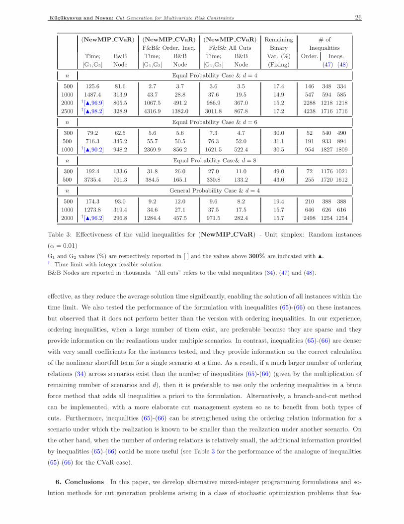
Kucukyavuz and Noyan: Cut Generation for Multivariate Risk Constraints 26
(NewMIP CVaR) (NewMIP CVaR) (NewMIP CVaR) Remaining # of
F&B& Order. Ineq. F&B& All Cuts Binary Inequalities
Time; B&B Time; B&B Time; B&B Var. (%) Order. Ineqs.
[G1,G2] Node [G1,G2] Node [G1,G2] Node (Fixing) (47) (48)
n Equal Probability Case & d = 4
500 125.6 81.6 2.7 3.7 3.6 3.5 17.4 146 348 334
1000 1487.4 313.9 43.7 28.8 37.6 19.5 14.9 547 594 585
2000 †[N,96.9] 805.5 1067.5 491.2 986.9 367.0 15.2 2288 1218 1218
2500 †[N,98.2] 328.9 4316.9 1382.0 3011.8 867.8 17.2 4238 1716 1716
n Equal Probability Case & d = 6
300 79.2 62.5 5.6 5.6 7.3 4.7 30.0 52 540 490
500 716.3 345.2 55.7 50.5 76.3 52.0 31.1 191 933 894
1000 †[N,90.2] 948.2 2369.9 856.2 1621.5 522.4 30.5 954 1827 1809
n Equal Probability Case& d = 8
300 192.4 133.6 31.8 26.0 27.0 11.0 49.0 72 1176 1021
500 3735.4 701.3 384.5 165.1 330.8 133.2 43.0 255 1720 1612
n General Probability Case & d = 4
500 174.3 93.0 9.2 12.0 9.6 8.2 19.4 210 388 388
1000 1273.8 319.4 34.6 27.1 37.5 17.5 15.7 646 626 616
2000 †[N,96.2] 296.8 1284.4 457.5 971.5 282.4 15.7 2498 1254 1254
Table 3: Effectiveness of the valid inequalities for (NewMIP CVaR) - Unit simplex: Random instances
(α = 0.01)
G1 and G2 values (%) are respectively reported in [ ] and the values above 300% are indicated with N.†: Time limit with integer feasible solution.
B&B Nodes are reported in thousands. “All cuts” refers to the valid inequalities (34), (47) and (48).
effective, as they reduce the average solution time significantly, enabling the solution of all instances within the
time limit. We also tested the performance of the formulation with inequalities (65)-(66) on these instances,
but observed that it does not perform better than the version with ordering inequalities. In our experience,
ordering inequalities, when a large number of them exist, are preferable because they are sparse and they
provide information on the realizations under multiple scenarios. In contrast, inequalities (65)-(66) are denser
with very small coefficients for the instances tested, and they provide information on the correct calculation
of the nonlinear shortfall term for a single scenario at a time. As a result, if a much larger number of ordering
relations (34) across scenarios exist than the number of inequalities (65)-(66) (given by the multiplication of
remaining number of scenarios and d), then it is preferable to use only the ordering inequalities in a brute
force method that adds all inequalities a priori to the formulation. Alternatively, a branch-and-cut method
can be implemented, with a more elaborate cut management system so as to benefit from both types of
cuts. Furthermore, inequalities (65)-(66) can be strengthened using the ordering relation information for a
scenario under which the realization is known to be smaller than the realization under another scenario. On
the other hand, when the number of ordering relations is relatively small, the additional information provided
by inequalities (65)-(66) could be more useful (see Table 3 for the performance of the analogue of inequalities
(65)-(66) for the CVaR case).
6. Conclusions In this paper, we develop alternative mixed-integer programming formulations and so-
lution methods for cut generation problems arising in a class of stochastic optimization problems that fea-
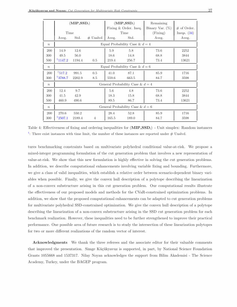
Kucukyavuz and Noyan: Cut Generation for Multivariate Risk Constraints 27
(MIP SSDl) (MIP SSDl) Remaining
Fixing & Order. Ineq. Binary Var. (%) # of Order.
Time Time (Fixing) Ineqs. (34)
Aveg. Std. # Unslvd Aveg. Std. Aveg. Aveg.
n Equal Probability Case & d = 4
200 14.9 12.6 5.9 5.8 73.6 2252
300 49.5 56.0 18.6 14.8 68.8 3844
500 †1147.2 1194.4 0.5 219.4 256.7 73.4 13621
n Equal Probability Case & d = 6
200 †517.2 991.5 0.5 41.0 87.1 85.9 1716
300 †3788.7 2202.9 8.5 559.6 663.5 84.7 3598
n General Probability Case & d = 4
200 12.4 9.7 5.6 4.8 73.6 2252
300 41.5 42.9 18.3 15.8 68.8 3844
500 460.9 490.6 89.5 86.7 73.4 13621
n General Probability Case & d = 6
200 270.6 550.2 28.4 52.8 85.9 1716
300 †2507.1 2189.4 4 165.5 189.0 84.7 3598
Table 4: Effectiveness of fixing and ordering inequalities for (MIP SSDl) - Unit simplex: Random instances†: There exist instances with time limit, the number of these instances are reported under # Unslvd.
tures benchmarking constraints based on multivariate polyhedral conditional value-at-risk. We propose a
mixed-integer programming formulation of the cut generation problem that involves a new representation of
value-at-risk. We show that this new formulation is highly effective in solving the cut generation problems.
In addition, we describe computational enhancements involving variable fixing and bounding. Furthermore,
we give a class of valid inequalities, which establish a relative order between scenario-dependent binary vari-
ables when possible. Finally, we give the convex hull description of a polytope describing the linearization
of a non-convex substructure arising in this cut generation problem. Our computational results illustrate
the effectiveness of our proposed models and methods for the CVaR-constrained optimization problems. In
addition, we show that the proposed computational enhancements can be adapted to cut generation problems
for multivariate polyhedral SSD-constrained optimization. We give the convex hull description of a polytope
describing the linearization of a non-convex substructure arising in the SSD cut generation problem for each
benchmark realization. However, these inequalities need to be further strengthened to improve their practical
performance. One possible area of future research is to study the intersection of these linearization polytopes
for two or more different realizations of the random vector of interest.
Acknowledgments We thank the three referees and the associate editor for their valuable comments
that improved the presentation. Simge Kucukyavuz is supported, in part, by National Science Foundation
Grants 1055668 and 1537317. Nilay Noyan acknowledges the support from Bilim Akademisi - The Science
Academy, Turkey, under the BAGEP program.
Kucukyavuz and Noyan: Cut Generation for Multivariate Risk Constraints 28
References
Armbruster, B. and Luedtke, J. (2015). Models and formulations for multivariate dominance constrained
stochastic programs. IIE Transactions, 47:1–14.
Dentcheva, D., Penev, S., and Ruszczynski, A. (2010). Kusuoka representation of higher order dual risk
measures. Annals of Operations Research, 181:325–335.
Dentcheva, D. and Ruszczynski, A. (2003). Optimization with stochastic dominance constraints. SIAM Journal
on Optimization, 14(2):548–566.
Dentcheva, D. and Ruszczynski, A. (2006). Portfolio optimization with stochastic dominance constraints.
Journal of Banking and Finance, 30(2):433–451.
Dentcheva, D. and Ruszczynski, A. (2009). Optimization with multivariate stochastic dominance constraints.
Mathematical Programming, 117:111–127.
Dentcheva, D. and Ruszczynski, A. (2010). Inverse cutting plane methods for optimization problems with
second-order stochastic dominance constraints. Optimization, 59(3):323–338.
Dentcheva, D. and Wolfhagen, E. (2015). Optimization with multivariate stochastic dominance constraints.
SIAM Journal on Optimization, 25(1):564–588.
Ehrgott, M. (2005). Multicriteria Optimization. Springer, Berlin.
Fabian, C., Mitra, G., and Roman, D. (2011). Processing second-order stochastic dominance models using
cutting-plane representations. Mathematical Programming, 130(1):33–57.
Hadar, J. and Russell, W. R. (1969). Rules for ordering uncertain prospects. The American Economic Review,
59(1):25–34.
Haskell, W., Shanthikumar, J., and Shen, Z. (2013). Optimization with a class of multivariate integral
stochastic order constraints. Annals of Operations Research, 206(1):147–162.
Homem-de-Mello, T. and Mehrotra, S. (2009). A cutting surface method for uncertain linear programs with
linear stochastic dominance constraints. SIAM Journal on Optimization, 20(3):1250–1273.
Hu, J., Homem-de-Mello, T., and Mehrotra, S. (2011). Risk-adjusted budget allocation models with application
in homeland security. IIE Transactions, 43(12):819–839.
Hu, J., Homem-de Mello, T., and Mehrotra, S. (2012). Sample average approximation of stochastic dominance
constrained programs. Mathematical Programming, 133(1-2):171–201.
Hu, J. and Mehrotra, S. (2012). Robust and stochastically weighted multiobjective optimization models and
reformulations. Operations Research, 60(4):936–953.
Luedtke, J. (2008). New formulations for optimization under stochastic dominance constraints. SIAM Journal
on Optimization, 19(3):1433–1450.
Noyan, N. and Rudolf, G. (2013). Optimization with multivariate conditional value-at-risk-constraints. Oper-
ations Research, 61(4):990–1013.
Noyan, N., Rudolf, G., and Ruszczynski, A. (2008). Relaxations of linear programming problems with first
order stochastic dominance constraints. Operations Research Letters, 34(6):653–659.
Rockafellar, R. and Uryasev, S. (2000). Optimization of conditional value-at-risk. The Journal of Risk,
2(3):21–41.
Rudolf, G. and Ruszczynski, A. (2008). Optimization problems with second order stochastic dominance
constraints: duality, compact formulations, and cut generation methods. SIAM Journal on Optimization,
19:1326–1343.

Kucukyavuz and Noyan: Cut Generation for Multivariate Risk Constraints 29
Willis, H. H., Morral, A. R., Kelly, T. K., and Medby, J. J. (2005). Estimating terrorism risk. Technical
report, The RAND Corporation, Santa Monica, CA.