Airfoil Design

Available Approaches

• Optimization Methods

• Inverse Design Methods

• Ad Hoc “Cut and Try Methods”

Optimization Theory I

x+y=1

x=0

y=0

P1P

P2

Black Boxx

y

f(x,y)

What combination of x and y will produce the lowest F(x,y)Subject to the constraints x > 0 , y > 0, x + y < 1 ?

Strategy

• Start at a point P. Compute F(x,y) at P

• Take a small step to the right, find F(x+x, y)

• Use this to find F/ x at P.

• Similarly find F/ y at P• Construct a gradient

vector .• Find new values of x,y

F

yF

yy

FxF

xx

ey

Fe

x

FF

y

xFyyxF

y

Fx

xFyxxF

x

F

Pnew

Pnew

21

)(),(

)(),(

Commonly Used Optimization Tools

• MATLAB has built-in functions!• Vanderplaats at NASA Ames Research

Center, developed a computer code is called CONMIN (Constrained Minimization); Reference NASA TMX62282, August 1973).

• NASA’s QNMDIF code which uses a similar methodology coupled with a Quasi-Newton iterative scheme.

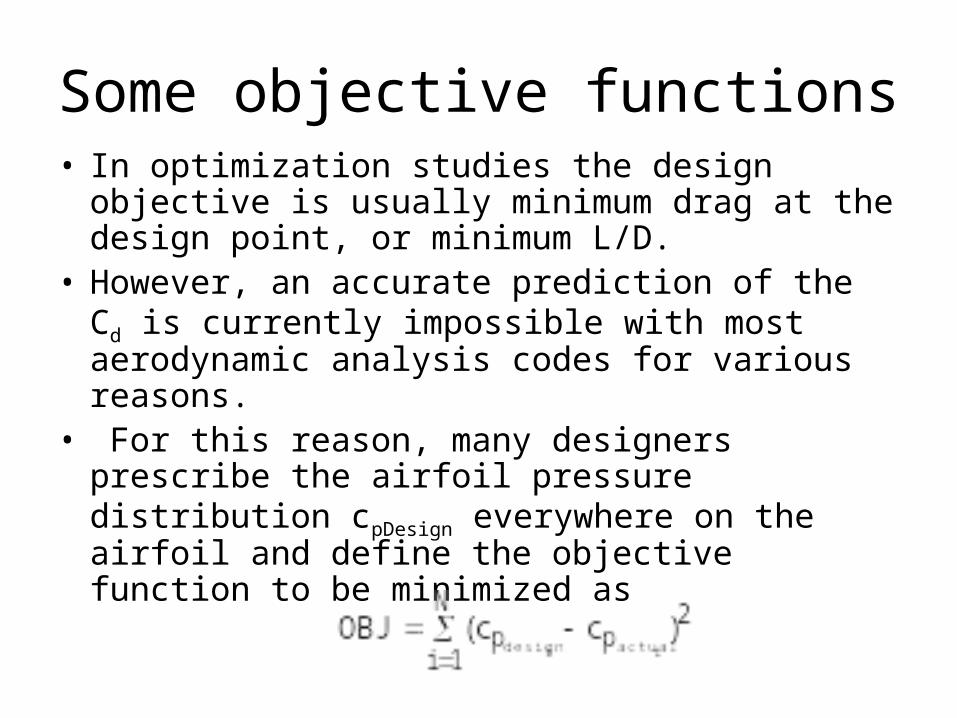
Some objective functions• In optimization studies the design objective is

usually minimum drag at the design point, or minimum L/D.

• However, an accurate prediction of the Cd is currently impossible with most aerodynamic analysis codes for various reasons.

• For this reason, many designers prescribe the airfoil pressure distribution cpDesign everywhere on the airfoil and define the objective function to be minimized as

Starting Point

• The starting point in the design process is a baseline airfoil shape that is known to produce a cp distribution close to the design cp distribution at the design Mach number and angle of attack.

• Some expertise is needed to establish a good starting point.

• Industries normally start with their best airfoil.

Airfoil coordinates asDesign Variables

• In an optimization problem, the design variables are the quantities whose values are adjusted until the objective function OBJ is minimized.

• In an airfoil design by optimization techniques, the obvious choice for design variables are the airfoil y-ordinates at certain fixed number of x-locations.

• One can adjust these individual y-ordinates until the objective function OBJ is minimized.

• Problem is… there are usually 100 or more design variables if we define the airfoil with 100 nodes. This is too many!

Alternate Design Variables

EXPONENT

TABLE

j n

4 0.5757166

5 0.7564708

6 1.0

7 1.356915

8 1.943358

9 3.106283

10 6.578813

TERM EQUATION

P(1)

P(2)

P(3)

P(J), J=4,10

P(11) x10

(Reference : NACA CR 3065 “Analysis of a Theoretically Optimized Transonic Airfoil”)

These functions are called “Bump” Functions

0

0.5

1

1.5

2

2.5

3

3.5

0 0.5 1 1.5

Series1

Series2

Series3

Series4

Design Constraints

• May be geometric:– Airfoil too thin or too thick..– Leading edge radius is too small, which may

lead to leading edge stall.

• May be performance related:– Good transonic performance as well as

supercruise performance desired.– Good cruise performance as well as high

enough Clmax for take-off / landing performance.

Black Box

Input

a(1)

a(2)

a(12)

.

.

.

.

M,

Computes New

Airfoil Shape

Preprocessor

New Airfoil Shape

M,

An a l y s i s

cp, cl, cd Post

Proc- essor

OBJ

OVERALL FLOW OF INFORMATION

Input : Design Variables

OBJ & Constraint Info

User-written Monitor Program

CONMIN Subroutines

Black Box

OBJ & Constraint Info

Input : Design Variables

Some Details..1. The monitor program needs the input baseline geometry, the free-stream Mach

number and angle of attack, and the design or target pressures, cpdesign. The main program also reads input regarding which of the 12 design variables are to

participate in the design. For example, let a3, a5 and a7 be the three design variables to be considered in the present design. All the other design variables and these three variables are initialized to zero.

2. Optimization routines, say CONMIN, send a3=0, a5=0 and a7=0 through the monitor program to the black box. The values of OBJ are returned.

3. CONMIN finds by perturbing each variable in turn and using finite-difference formulae to evaluate the derivatives as discussed previously.

4. Based on the information from step 3, CONMIN chooses changes to a3, a5 and a7 which will cause OBJ to decrease. These changes are added to a3, a5, a7 to get new updated , etc.

5. CONMIN sends the new and receives the new OBJ from the black box.6. CONMIN goes to step 3. Steps 3 through 6 are repeated as man times as needed, as

specified by the user.7. The monitor program prints out the final airfoil shape corresponding to the final airfoil

design variable values, and stops. The design cp and the actual cp are sometimes printed out to ensure that the final airfoil does generate cp values close to the design values.

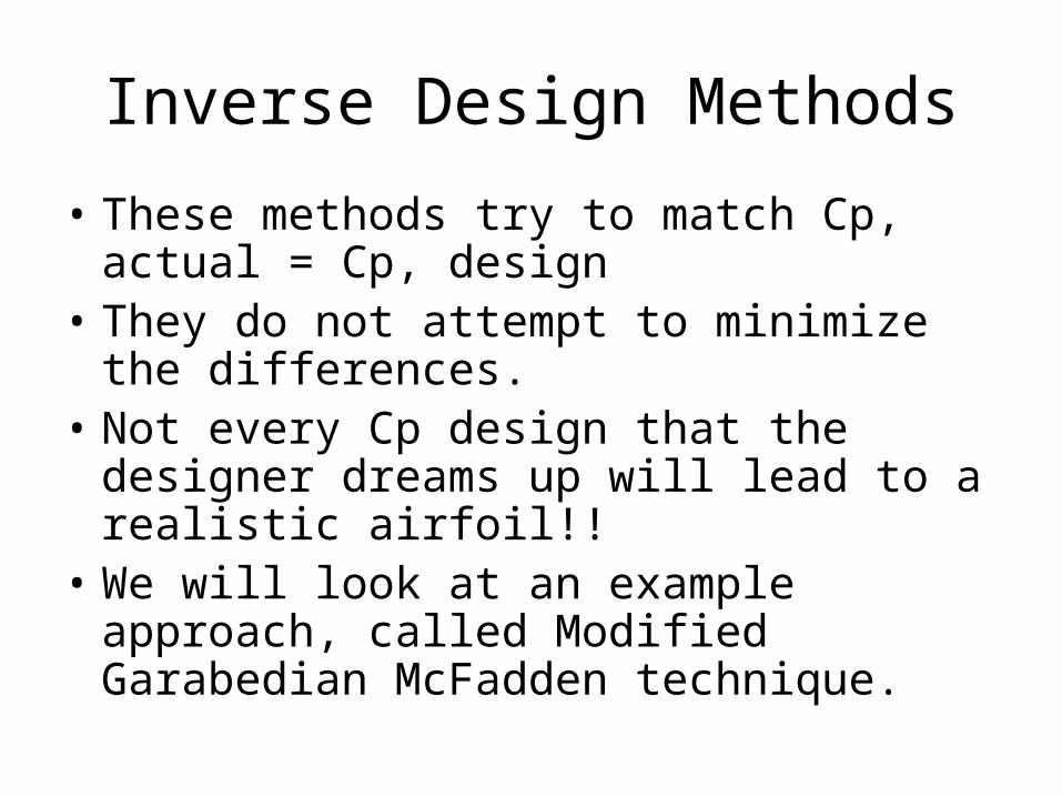
Inverse Design Methods

• These methods try to match Cp, actual = Cp, design

• They do not attempt to minimize the differences.

• Not every Cp design that the designer dreams up will lead to a realistic airfoil!!

• We will look at an example approach, called Modified Garabedian McFadden technique.

What is this method?

• It is a method for designing airfoils and wings, given a target pressure distribution.

• It was originally developed by Garabedian and McFadden for use in a very specific application- wing design in a code called FLO22.

• It was extended for use with any analysis (Panel, CFD) and any configuration (wing, airfoil, fuselage..) by Malone and Sankar at Lockheed.

• It has been used in rotor blade design by Narramore (Bell), and Hassan (Boeing Mesa).

Principles behind this method

• The surface pressure distribution, or the flow velocity on the surface (i.e. just outside the boundary layer) will depend on the surface slope dZ/dx, the surface ordinate Z and the surface second derivative d2Z/dx2.

• Thus, changes in the pressure or speed between present values and target values will depend on changes to Z, changes to slope, and changes to the second derivative.

Principles (Continued..)

Z

Original Airfoil

Target Airfoil

Original Velocity

Target Velocity

V

V2 = Function of (Z, dZ/dx, d2Z/dx2)

Change in velocity squared at the surface

The equation solved

A Z + B d(Z)/dx + C d2(Z)/dx2 = V2 target – V2 present

This equation is not physically based.

The Cp on the airfoil is a more complicated function of surface slope, curvature, and ordinates.

However, for deciding how the Z coordinates of a given airfoil should be changed, the above equation will do.

A, B, C are arbitrary constants. These should be large enough to keepThe airfoil from changing too much. – We usually set these to A=B=C=10.

When target velocities approach present velocities, the airfoil stops changing.

That is, when the right hand side goes to zero, Z goes to zero.

APPROACH• Convert target Cp values to target Velocity squared. Interpolate the

target velocities to the panel edges, or to the (x,y) locations of the airfoil on the CFD grid. This is done only once. This may be done using a spreadsheet or MATLAB.

• Start with a given airfoil. Analyze it. Convert Cp values to squares of velocity at the edges (Panel) or the (x,y) points on the airfoil (CFD).

• Compute the difference between target velocities and computed velocities at these points on the airfoil (e.g. mid-points of panels, or the 81 points on the CFD grid).

• Solve equation in the previous slide to compute Z.

• Add this Z to the airfoil you started with. This becomes your new airfoil.

• Repeat these steps until Z becomes small, and the Cp values from your analysis begin to look like the target Cp values.

How do we convert Cp to velocity_squared?

• In incompressible flow, this is easy.– Cp = 1- Velocity^2

• In compressible flow, one needs to use isentropic energy equation.

1 1

2M

2 1u2 v2

V2

1

1Cp

p p1

2V

2

p

p 1

2

M2

1

2

M2

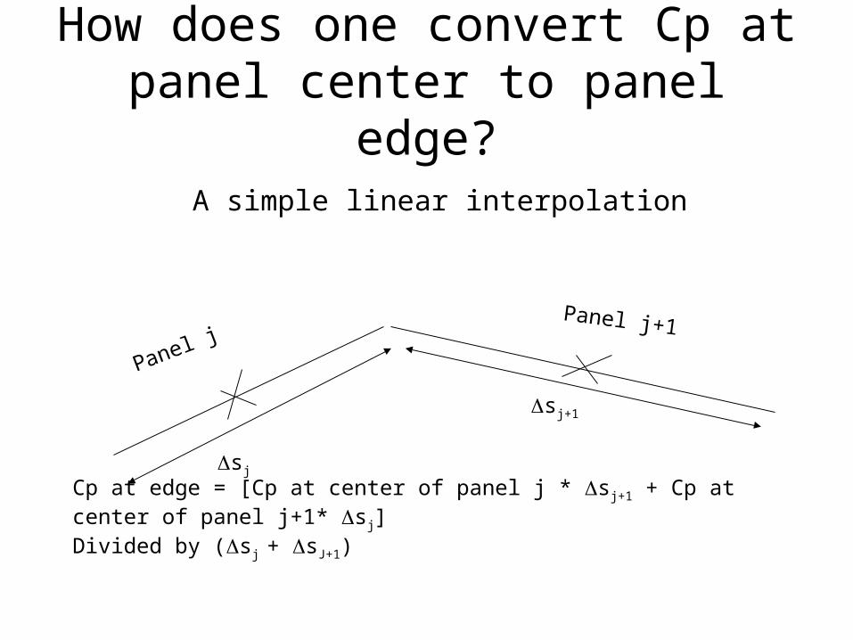
How does one convert Cp at panel center to panel edge?

Panel jPanel j+1

sj

sj+1

Cp at edge = [Cp at center of panel j * sj+1 + Cp at center of panel j+1* sj]Divided by (sj + sJ+1)

A simple linear interpolation

How does one solve the MGM equation?

• It is briefly described in a paper given as a handout last week.

• The procedure looks complicated, but is extremely simple. (Famous last words..)

Numerical details

ii

ii

xx

ZZ

x

Z

1

1

Approximation of d(Z)/dx on the upper surface:

i-1

ii+1

Approximation of d(Z)/dx on the lower surface:

i+1 ii-1

1

1

ii

ii

xx

ZZ

x

Z

Numerical DetailsApproximation of d2(Z)/dx2 on the upper surface:

i-1

ii+1

211

1

1

1

1

2

2

ii

ii

ii

ii

ii

xxxxZZ

xxZZ

x

Z

With these approximations..

A Z + B d(Z)/dx + C d2(Z)/dx2 = V2 target – V2 actual

Becomes

2iActual,

2iTarget,

11

1

1

1

1

1

1 2 VVxx

xxZZ

xxZZ

Cxx

ZZBZA

ii

ii

ii

ii

ii

ii

iii

On the upper surface.

A similar equation occurs on the lower surface.

At the leading and trailing edges, we set Z to zero.

This above system of equations is linear, sparse, and tri-diagonal.

It is easily inverted with a variant of Gaussian elimination called Thomas algorithm.

Test Case

• Start with a NACA 0012 airfoil.• Supply the pressure distribution on NACA

4412 airfoil as the desired target values.• See if the design process smoothly

changes the shape from 0012 to 4412.• This test is usually assigned as a

homework problem in 3903.• Panel code/CFD code supplied (see 3903

web site), students write the design code..

Airfoil shape converges to expected values

-0.15

-0.1

-0.05

0

0.05

0.1

0.15

0 0.1 0.2 0.3 0.4 0.5 0.6 0.7 0.8 0.9 1

x/c

y

NACA 4412 iteration25

Pressure Distribution on final shape is very close to target values

-1.5

-1

-0.5

0

0.5

1

1.5

0 0.1 0.2 0.3 0.4 0.5 0.6 0.7 0.8 0.9 1

x/c

cp

cptarget iteration25

Design Case• Design a transonic airfoil that generates a Lift

coefficient of 0.6 at Mach .75 with no shock waves.– Step 1: Construct a target pressure distribution.

This requires some experience.– Step 2: Analyze this pressure distribution with a

compressible boundary layer analysis to make sure that the airfoil will not stall or separate prematurely.

– Step 3: Run design code with this target pressure distribution

-1.5

-1

-0.5

0

0.5

1

1.5

0 0.1 0.2 0.3 0.4 0.5 0.6 0.7 0.8 0.9 1

x/c

Cp

• Design Consideration-No Shock or Weak Shock– Rapid rise to large

pressure at leading edge– Relatively flat over large

portion of chord– Smooth transition at

leading edge– A large favorable pressure

gradient region is desirable.

Target Pressure Distribution

Results

• Retrieved Pressure distribution-65 iterations

-1.50E+00

-1.00E+00

-5.00E-01

0.00E+00

5.00E-01

1.00E+00

0 0.1 0.2 0.3 0.4 0.5 0.6 0.7 0.8 0.9 1

x/c

Cp,y/c

airfoil shape final airfoil (iteration 62) cptarget

Concluding Remarks

• Airfoil Design is an interesting field.• It is relatively straightforward to design 2-D

airfoils, using optimization methods or inverse design methods.

• The only tools one needs are– Potential flow analyses– Boundary layer analyses– Small programs that implement the design strategy.

• See you all in my AE 4903 class next fall, for some hands-on experience!