Culture, Rationalisation and Corruption - UNSW Business … · Everyone was doing it: Culture,...
72
Everyone was doing it: Culture, Rationalisation and Corruption Patrick Schneider Supervised by Dr Gautam Bose School of Economics, The University of New South Wales 24 October 2011 Submitted in partial fulfilment of the requirements of the degree of Bachelor of Economics with Honours
Transcript of Culture, Rationalisation and Corruption - UNSW Business … · Everyone was doing it: Culture,...
Everyone was doing it:
Culture, Rationalisationand Corruption
Patrick Schneider
Supervised by Dr Gautam Bose
School of Economics,
The University of New South Wales
24 October 2011
Submitted in partial fulfilment of the requirements of the degree
of
Bachelor of Economics with Honours

I hereby declare that this submission is my own work and to the best of
my knowledge it contains no materials previously published or written
by another person, or substantial proportions of material which have
been accepted for the award of any other degree or diploma at UNSW or
any other educational institution, except where due acknowledgement is
made in the thesis. Any contribution made to the research by others, with
whom I have worked at UNSW or elsewhere, is explicitly acknowledged
in the thesis.
I also declare that the intellectual content of this thesis is the product
of my own work, except to the extent that assistance from others in the
project’s design and conception or in style, presentation and linguistic
expression is acknowledged.
Patrick Schneider

Acknowledgments
I am incredibly grateful to Gautam Bose, my supervisor, for his openness, reassurance
and guidance at every stage throughout the year. I am also extremely grateful to Zhanar
Akhmetova and Alberto Motta who helped me find direction in my argument in the em-
pirical and theoretical sections respectively.
Two of my friends proof-read the thesis and provided helpful feedback throughout the
year as well. They are Susie Kaye and Patrick Hurley and I extend my thanks to them.
ii

Contents
Abstract 1
1 Introduction 2
2 Corruption 4
2.1 The Nature and Impact of Corruption . . . . . . . . . . . . . . . . . . . . 4
2.2 The Causes of Corruption . . . . . . . . . . . . . . . . . . . . . . . . . . . 5
2.2.1 Theoretical models of corruption . . . . . . . . . . . . . . . . . . . 5
2.2.2 Empirical models of corruption . . . . . . . . . . . . . . . . . . . . 7
3 Corruption and Social Psychology 10
3.1 Corruption as an Immoral Act . . . . . . . . . . . . . . . . . . . . . . . . . 10
3.2 Rational Choice and Morality . . . . . . . . . . . . . . . . . . . . . . . . . 11
3.3 Social Influence and Personal Morality . . . . . . . . . . . . . . . . . . . . 13
4 Theoretical Model 16
4.1 Discussion . . . . . . . . . . . . . . . . . . . . . . . . . . . . . . . . . . . . 17
4.2 Model . . . . . . . . . . . . . . . . . . . . . . . . . . . . . . . . . . . . . . 18
4.2.1 General form . . . . . . . . . . . . . . . . . . . . . . . . . . . . . . 18
4.2.2 Closed form . . . . . . . . . . . . . . . . . . . . . . . . . . . . . . . 20
4.2.3 Extensions . . . . . . . . . . . . . . . . . . . . . . . . . . . . . . . . 24
5 Data 29
5.1 Corruption Data . . . . . . . . . . . . . . . . . . . . . . . . . . . . . . . . 29
5.1.1 Country level perception indices . . . . . . . . . . . . . . . . . . . . 29
5.1.2 Country level experience indices . . . . . . . . . . . . . . . . . . . . 31
5.1.3 Department level experience indices . . . . . . . . . . . . . . . . . . 32
5.2 Other Data . . . . . . . . . . . . . . . . . . . . . . . . . . . . . . . . . . . 34
5.2.1 Variables of interest . . . . . . . . . . . . . . . . . . . . . . . . . . . 34
5.2.2 History controls . . . . . . . . . . . . . . . . . . . . . . . . . . . . . 36
5.2.3 Instruments . . . . . . . . . . . . . . . . . . . . . . . . . . . . . . . 36
iii

CONTENTS Patrick Schneider
6 Empirical Specifications 37
6.1 Distribution . . . . . . . . . . . . . . . . . . . . . . . . . . . . . . . . . . . 38
6.2 Tests . . . . . . . . . . . . . . . . . . . . . . . . . . . . . . . . . . . . . . . 39
6.2.1 Within country comparison—sign test . . . . . . . . . . . . . . . . 39
6.2.2 Cross country comparison—regressions . . . . . . . . . . . . . . . . 41
7 Results 44
7.1 Department Level Variation in Corruption . . . . . . . . . . . . . . . . . . 44
7.1.1 Systematic department e↵ects . . . . . . . . . . . . . . . . . . . . . 44
7.1.2 Idiosyncratic department e↵ects . . . . . . . . . . . . . . . . . . . . 46
7.2 Cross-Country Regression Estimation . . . . . . . . . . . . . . . . . . . . . 46
7.2.1 Baseline model . . . . . . . . . . . . . . . . . . . . . . . . . . . . . 48
7.2.2 Model 1 . . . . . . . . . . . . . . . . . . . . . . . . . . . . . . . . . 48
7.2.3 Model 2 . . . . . . . . . . . . . . . . . . . . . . . . . . . . . . . . . 50
7.3 Limitations . . . . . . . . . . . . . . . . . . . . . . . . . . . . . . . . . . . 54
8 Conclusion 56
A Appendix 58
A.1 Skewness and Kurtosis Test for Normality . . . . . . . . . . . . . . . . . . 58
A.2 Sign Test on Department Level Corruption Results . . . . . . . . . . . . . 59
A.3 Two Stage Least Squares Regressions . . . . . . . . . . . . . . . . . . . . . 61
iv
List of Figures
4.1 Equilibrium ⇤ with and without supervision . . . . . . . . . . . . . . . . . 26
5.1 Comparison of Perception Indices . . . . . . . . . . . . . . . . . . . . . . . 30
5.2 Comparison of Experience and Perception Indices . . . . . . . . . . . . . . 32
6.1 GCB 2010 and ES 2009—Department Kernel Densities . . . . . . . . . . . 40
7.1 GCB 2010 and ES 2009—Corruption Di↵erences for Idiosyncratic Rela-
tionships . . . . . . . . . . . . . . . . . . . . . . . . . . . . . . . . . . . . . 47
v
List of Tables
5.1 Descriptive statistics for corruption measures . . . . . . . . . . . . . . . . . 31
5.2 Correlation between country level corruption indices . . . . . . . . . . . . . 33
5.3 Department level GCB 2010 (No bribe) . . . . . . . . . . . . . . . . . . . . 34
5.4 Descriptive statistics for independent variables . . . . . . . . . . . . . . . . 35
6.1 Correlations between GCB departments . . . . . . . . . . . . . . . . . . . 38
7.1 Pairwise relationships (column � row) between departmental corruption
implied by sign test . . . . . . . . . . . . . . . . . . . . . . . . . . . . . . . 45
7.2 Country level regressions with logged dependent . . . . . . . . . . . . . . . 49
7.3 Department level regressions with logged dependent . . . . . . . . . . . . . 51
7.4 Model 2a results with di↵erent lags . . . . . . . . . . . . . . . . . . . . . . 53
A.1 GCB 2010 . . . . . . . . . . . . . . . . . . . . . . . . . . . . . . . . . . . . 58
A.2 ES 2009 . . . . . . . . . . . . . . . . . . . . . . . . . . . . . . . . . . . . . 58
A.3 Two-tailed p-values – H1 : median of Yi �Xi 6= 0 . . . . . . . . . . . . . . 59
A.4 One-tailed p-values – H1 : median of Yi �Xi > 0 . . . . . . . . . . . . . . 59
A.5 One-tailed p-values – H1 : median of Yi �Xi < 0 . . . . . . . . . . . . . . 59
A.6 Two-tailed p-values – H1 : median of Yi �Xi 6= 0 . . . . . . . . . . . . . . 60
A.7 One-tailed p-values – H1 : median of Yi �Xi > 0 . . . . . . . . . . . . . . 60
A.8 One-tailed p-values – H1 : median of Yi �Xi < 0 . . . . . . . . . . . . . . 60
A.9 2SLS Regressions . . . . . . . . . . . . . . . . . . . . . . . . . . . . . . . . 61
vi
Abstract
Microeconomic models of corruption tend to suggest that if bureaucrats face an opportu-
nity to be corrupt and the expected benefits are positive, they will take it. Drawing on the
criminology and social psychology literature, I propose a model of bureaucratic corrup-
tion that incorporates another important mechanism: cognitive dissonance that creates
the need to rationalise behaviour. Bureaucrats living in a society with a strong social
norm against corruption may or may not be able to rationalise, and therefore engage in,
corrupt behaviour. Their ability to do so depends on the organisational culture of the de-
partment they work in as well as the norms of society as a whole. The model has multiple
equilibria, which suggests that we should observe idiosyncrasies in the corruption levels
in government departments within countries, driven by these organisational cultures. We
should further observe that these cultures persist over time as new recruits are brought
into the fold by their veteran colleagues.
Analysis of newly available, disaggregated data on bribery in government depart-
ments finds patterns that support the implications of the theoretical model. This finding
is robust to controls for systematic department e↵ects and the department’s historical
corruption level, as well as for standard country level institutional and economic regres-
sors. The analysis elucidates some important correlates of corruption and also shows that
a department’s history is a strong predictor of its current corruption level. These findings
match the implications of the theoretical model.
1

Chapter 1
Introduction
We often talk about a ‘culture’ of corruption. We use the term to explain why four of
the last eight governors of Illinois have criminal convictions1, why you can expect to have
to pay a bribe for many government services in India (Bertrand, Djankov, Hanna, and
Mullainathan, 2007; Wade, 1982), and why development e↵orts in Africa are often so
unsuccessful (Moyo, 2009; Sardan, 1999). But although we lay the blame for corruption
at culture’s doorstep, our discussions rarely identify what, exactly, we mean.
Could it be that India, a country of a billion souls, has such a single unifying streak?
If so, why the constant protests and outpouring in the media against corruption2? The
identification of culture as something that only occurs at the national level is probably
not helpful. This thesis conceptualises culture as something that is developed by groups
of people. Thus although national cultures exist, others such as those that develop within
organisations are also of great importance to individuals.
There is a long literature within economics that models the decisions of government
o�cials3. These describe corruption as a result of the incentives o�cials face and have
been helpful in designing prevention programs4. This thesis extends this literature by
asking how the morals that o�cials hold and the cultures to which they are exposed can
a↵ect their decisions when they have the opportunity to be corrupt. It has been observed
that corruption does the most harm when it is an institutionalised part of government
processes, rather than the individual acts of a few bad apples. Hence, an understanding
of the links between corrupt agents and how these links serve to institutionalise corrupt
practices would add a beneficial foundation for anti-corruption e↵orts.
My thesis makes a theoretical contribution to the corruption literature by developing
a model that uses the methodology of past economic models, which tie corruption to
incentives, but is founded on a rich discussion of criminal behaviour and motivation from
the criminology and social psychology fields. The result is a model that explains individual
1Rod Blagojevich (2003-09), George H. Ryan (1999-2003), Dan Walker (1973-77) and Otto Kerner,Jr (1962-68).
2Witness the recent protest movement led by Anna Hazare, see http://www.economist.com/node/
21526904 accessed 17/10/20113Starting with Rose-Ackerman (1978).4See, for example, Klitgaard (1988).
2

CHAPTER 1. INTRODUCTION Patrick Schneider
corruption in terms of o�cials’ personal morals, which are shaped by interactions with
their colleagues and broader society.
The theoretical analysis finds that an o�cial’s personal choice of morals will tend
to conform to those chosen by his colleagues. However, if his perception of what is the
moral norm is imperfectly based on the the norms of his colleagues and those of roader
society, there are multiple moral lines that he and his colleagues could coordinate on
in equilibrium. Thus, a corrupt culture develops in a government department, but the
cultures across departments need not be the same5. Furthermore, if the o�cial bases his
perceptions on his colleagues’ behaviour in the past, then these cultures will be highly
persistent. It is notable that the multiple coordinated equilibria and persistence of culture
are independent of incentives. Although the latter a↵ect decisions in the model as well,
they do not interfere with the main findings.
The second contribution made by this thesis is in testing the implications of the
model by using a cross-country dataset of people’s experiences of paying bribes to di↵erent
departments. This dataset has not been used in the empirical literature before. The use
of department level data allows me to extend the past literature by controlling for the
inherent corruptibility of a department’s work, as well as other known correlates. I employ
two approaches to testing the implications. The first approach analyses relationships
between departments within the same country using the sign test and finds that the
noisy relationships predicted by the theoretical model do indeed obtain. The second
approach analyses cross-country variation in departmental corruption using two models.
The first model controls for country and department e↵ects and finds that the noise
predicted by the theoretical model is observable. The second model adds a lag of the
department’s corruption level and finds it to be significant, which supports the prediction
that departmental corruption will be persistent.
The thesis is structured as follows. Chapter 2 provides an overview of the main
trends and findings of economic research into corruption, both from a theoretical and
empirical perspective. Chapter 3 draws on the social psychology literature to provide an
in-depth analysis of how moral considerations a↵ect decision making for individuals that
act within social environments. Chapter 4 then incorporates these factors into a formal
theoretical model of corruption which is able to explain the variation and persistence
of corruption in an organisation as phenomena that are independent of the associated
incentive structure. These implications are then tested in the empirical section. Chapters
5 and 6 outline the data and strategy, respectively, that are used in the empirical analysis,
and results are presented in Chapter 7. Chapter 8 concludes.
5This provides intuition for why so many Illinois governors, but none from Indiana, have criminalconvictions.
3

Chapter 2
Corruption
2.1 The Nature and Impact of Corruption
Corruption is defined in various ways. The broadest and most widely used definition is
that corruption is the use of public o�ce for private gain (Bardhan, 1997; Gupta, Davoodi,
and Alonso-Terme, 2002; Shleifer and Vishny, 1993; You and Khagram, 2005). Another,
clearer, definition is that corruption is the violation of the duty of public o�ce for private
gain (Bac, 1996; Frank and Schulze, 2000; Khan, 1996; Sardan, 1999). Although the aspect
of violation of duty is likely intended by most, it is necessary to include it in the definition
to distinguish between bad policy and bad implementation of policy1, although the former
can be caused by corruption. The acts themselves may take a variety of forms—bribery,
embezzlement, extortion, diversion of funds—and occur in a variety of spheres—political
or bureaucratic. This thesis’ focus is on acts of bribery at the bureaucratic level.
Various theories of the impact of corruption abound and can be generally classed as
‘grease’ or ‘sand’ theories (Bardhan, 1997). That is, proponents of either side argue that
corruption acts as grease in the wheels of government, speeding up ine�cient processes
and enhancing welfare, or sand, creating friction in the wheels of government, introducing
ine�ciency into processes and diminishing welfare.
The most commonly cited proponent of the grease theory is Le↵ (1964), who argues
that “. . . corruption provides the insurance that if the government decides to steam full-
speed ahead in the wrong direction, all will not be lost. . . ” (p.11). A mundane example of
this could be where some resource is allocated by a queue or some other ine�cient mech-
anism. Corruption of this system might introduce an auction style sell-o↵, sending the
resource to the person with the highest willingness to pay, increasing e�ciency. Although
it may be true that a particular corrupt act may serve some benefit somewhere, detailed
case studies and data analysis in more recent years have shown that such occurrences are
overwhelmingly exceptions to the norm (Klitgaard, 1988, pp. 30-38). Furthermore, if one
broadens the scope of analysis beyond the specific corrupt act, it is highly likely that the
costs it creates will outweigh any benefits (Rose-Ackerman, 1978, p. 95).
1For example, the tax farming systems used by the Roman and Ottoman Empires would be consideredcorrupt by the first definition but not by the second.
4

CHAPTER 2. CORRUPTION Patrick Schneider
Theories and evidence for the sand theory are much more readily available. Cor-
ruption can negatively a↵ect the social and power structure of a society by entrenching
incumbent players (Shleifer and Vishny, 1993) and power figures (Khan, 1996) as well as
inducing or exacerbating inequality (Gupta et al., 2002; You and Khagram, 2005). This
can lead to brittle institutions that are unable to provide services (Wade, 1982), unwilling
to adapt (Johnston, 2005) or that undermine innovation (Murphy, Shleifer, and Vishny,
1993). It can waste resources by diverting them into rent-seeking (Krueger, 1974; Mur-
phy et al., 1993; Sardan, 1999) or covering up corrupt activity (Blackburn, Bose, and
Haque, 2006). And it can reduce investment by imposing an extra cost (Maitland, 2001;
Mauro, 1995) or by increasing uncertainty and thereby undermining incentives to invest
(Maitland, 2001; Mauro, 1995).
The work by economists on the impact of corruption is largely theoretical. Where
it is not, the empirical analysis tends to be of a more general nature; e.g. establishing
a causal relationship between corruption and investment. This is probably a result of
the data that are available—corruption indices tend to be problematic, there are very
few valid instruments and countrywide data on the impact factors discussed in theory
are hard to come by2. Furthermore, the main goal in researching corruption seems to be
to reduce the phenomenon. To this end, the assumption that corruption is a burden on
society (contemporarily taken to be “ . . . a well-proven fact. . . ” (Dusek, Ortmann, and
Lizal, 2005)) is enough to be a motivating force behind research into identifying its causes,
the focus of this thesis.
2.2 The Causes of Corruption
Various causal mechanisms for corruption have been suggested and studied in recent years.
The following outlines some of the key features of the empirical and theoretical work in
this area.
2.2.1 Theoretical models of corruption
There are various theoretical models of corruption that focus on di↵erent mechanisms
and e↵ects. At the core of most models is the familiar principle-agent framework where
the agent is a bureaucrat or politician and the principle a senior or the general public.
Corruption arises when perverse incentives, combined with an ability for the agent to hide
his actions, make corrupt behaviour a dominant strategy. A simple illustrative example is
provided by Klitgaard (1988, pp. 69-74). In his model, agents are paid a wage to deliver
a service to the public. They have a choice of being corrupt (in which case they receive
an extra payment) or not. If they are corrupt, they exact negative externalities on their
principle. Their principle hence makes e↵orts to catch them, but is only successful with
some probability. When a corrupt agent is caught, they must pay a fine. In Klitgaard’s
2To be discussed more fully in Chapter 5.
5

CHAPTER 2. CORRUPTION Patrick Schneider
model, agents also su↵er a moral cost if they choose to be corrupt, this is a fixed amount
that marginally reduces the incentive for corruption.
Another, more complicated, example of a principle-agent based model comes from
Bac (1996). He proposes a basic principal-agent framework but focuses on the role of su-
pervision. He notes that most of the agency literature on corruption takes the institutional
structure as given and focuses on organising the right agreement between principal and
agent to induce the desired behaviour. His article takes the opposite approach by fixing
incentives and varying the institutional structure to determine the comparative e↵ective-
ness of di↵erent models of supervision on limiting corruption. He finds that where there
are low variable costs to monitoring, it pays to have very horizontal supervision structures
(one supervisor to many agents). Where this applies with thresholds, the group of agents
need be split into groups and supervised in the same way. Where variable costs become
significant, however, there is no generally optimal structure and the explicit monitoring
costs need be identified.
Some models extend beyond the purely micro principle-agent framework in an at-
tempt to explain macro phenomena. Blackburn et al. (2006), for example, propose a
dynamic, general equilibrium model that incorporates a principle-agent framework to de-
velop a theoretical basis for the observed two-way causal relationship between corruption
and development. Their model incorporates a government, bureaucrats and households
whose decisions are interrelated. In the model, corruption acts as a drag on development
because resources are wasted trying to hide the transgressions. In the other direction,
development a↵ects corruption because it is linked to bureaucrats’ wages (the richer the
country, the better paid the bureaucrats) so in more developed countries, bureaucrats
have more to lose from corruption and there is hence less. There are two equilibria,
one with high corruption and low development, and one with low corruption and high
development.
Those models that analyse corruption at higher levels than the principle-agent re-
lationship tend to share this feature of multiple equilibria3. Another example is from
Murphy et al. (1993). This is a more abstract and simpler model than those consid-
ered above. In their setup, people simply have a choice of three occupations—market
production, subsistence production or rent-seeking (appropriating market production).
They show that where there are increasing returns to rent-seeking, multiple equilibria
will emerge—a stable point with everyone choosing market production over rent-seeking
or subsistence production, another stable point with high rent-seeking and people indif-
ferent between market and subsistence production and an unstable point where people
are indi↵erent between rent-seeking and market production.
Few models incorporate any moral aspect to the decision to become corrupt. Agents
are simply faced with a choice between alternatives that carry costs, benefits and risks
and choose to maximise their narrowly defined expected utility. Viewed in this light, the
3Multiple equilibria are present in some agent level analyses as well. See, for example, Nabin and Bose(2008).
6

CHAPTER 2. CORRUPTION Patrick Schneider
decision process an agent goes through when choosing between being corrupt or not is
identical to his weighing a simple gamble. Some models do incorporate morality, usually
by giving agents exogenously defined, heterogenous personal corruptibility—for example,
Blackburn et al. (2006) and Bose and Gangopadhyay (2009) have both corruptible and
incorruptible agents—or adding a fixed ‘moral cost’ to choosing to be corrupt—for ex-
ample, Klitgaard (1988). These attempts recognise the unique nature of the decisions in
question; but the modifications are generally made without addressing the mechanisms
behind them and without focus on their implications.
One of the initial motivations for my research was that it seemed appropriate to place
agents within a moral structure that they have to take into account when making decisions.
Hence, my theoretical discussion in Chapters 3 to 4 proposes a model of corruption that
takes into account moral processes that are given a detailed theoretical foundation.
2.2.2 Empirical models of corruption
Since the seminal work by Mauro (1995) that used an index of perceived corruption in an
empirical analysis for the first time, there have been multiple studies using data to analyse
the causes of corruption. Most studies set out to test a single hypothesised relationship,
controlling for others, and find various interesting results, some examples of which follow:
� Ades and Di Tella (1999) argue that economies where there are higher rents will
have higher corruption because the gains from the activity are higher. It follows
that countries that are less open to trade should have higher corruption due to the
lower level of competition in the marketplace. They find that greater openness to
trade, measured by imports as a proportion of GDP, is a significant determinant of
perceived corruption.
� Fisman and Gatti (2002) argue that decentralisation of government power means of-
ficials will be more closely linked with the constituencies they serve, causing greater
accountability and therefore less corruption. They find that decentralisation, mea-
sured by subnational government expenditure over the total, is a significant deter-
minant of perceived corruption.
� Brunetti and Weder (2003) argue that a free press acts as a constraint against
corruption because o�cials can expect to be publicly outed if they are identified.
Therefore, countries with greater freedom of the press should experience lower levels
of corruption. They found that press freedom, measured by Freedom House’s index,
is indeed a significant determinant of perceived corruption.
� You and Khagram (2005) argue that inequality fractures society and that the larger
the gap between rich and poor, the more the rich seek extra-legal means like corrup-
tion to maintain their position. They find that inequality is a significant determinant
of perceived corruption.
7

CHAPTER 2. CORRUPTION Patrick Schneider
� Aidt, Dutta, and Sena (2008) argue that economic growth should reduce corruption
because o�cials know there will be more to extract in next period, causing them to
wait until then to extort their share so as to not risk missing out. They find that
economic growth is a significant determinant of perceived corruption, though this is
dependent on the strength of accountability institutions.
Daniel Treisman published a comprehensive survey of this literature, appropriately
titled What Have We Learned About the Causes of Corruption From Ten Years of Cross-
National Empirical Research? (Treisman, 2007). In this paper, he summarises the various
relationships that have been proposed and found to have a significant relationship with
corruption levels. He then reproduces these studies to identify which relationships are
robust to di↵erent measures of corruption and the inclusion of various controls. He es-
tablishes that an overwhelming amount of the variation in perceptions indices can be
explained using a set of robust variables. In his most successful regression, he records an
R2 of 92% (Treisman, 2007, pp. 233-34, regression (7)). The explanatory variables for
corruption (here measured using the World Bank’s Control of Corruption Index 2005) that
are found to have significant relationships in this regression are the log of GDP per capita
in purchasing power parity terms, fuel exports as a proportion of merchandise exports,
the year a country opened to trade, the time it takes to open a firm, whether a country
is an old democracy, whether a country is a presidential democracy, the extent of press
freedom, the proportion of women in government, newspaper circulation and controls for
religion, colonial history and legal tradition.
All the empirical studies discussed so far used one type of corruption measure—
perception indices. These are created by organisations that conduct surveys and ask
respondents how corrupt they believe a country to be. Being based on opinion, there are
various issues with these data, as Treisman and others readily recognise4. An alternative
measure that has become available in more recent years is called an experience index.
These are created by asking survey respondents questions about their personal experiences
with defined acts of corruption, usually bribery.
In his survey article, Treisman does his analysis using both perceptions and experi-
ence indices. Although his models using the former have extremely high predictive power
and many significant relationships, his work using the same variables on the latter yield
very little. Predictive power remains high, albeit not as high, but significant relationships
are scarce, often weak and not robust to controls.
We can conceptualise perception and experience based indices of corruption as mea-
suring di↵erent things. Perception indices (insofar as they are reliable) measure a broad
range of activities whereas experience indices measure specific acts. Hence, experience in-
dices measure a subset of the activities measured by perceptions indices. It is thus to be
expected that some relationships identified in regressions with perceptions indices are not
be present with experience based ones. For example, the restrictions of a free press would
4To be discussed in greater depth in Chapter 5.
8

CHAPTER 2. CORRUPTION Patrick Schneider
assumedly constrain high level political actors much more than the low level bureaucrats
measured by experience indices. It is therefore unsurprising that this relationship is not
found to be robust to the change of dependent variable. Other di↵erences, however, can-
not be expected on these grounds. For example, why would the rents available in the
home market (measured using the year opened to trade) a↵ect broad corruption but not
low-level bribery?
One of the initial motivations for my research was this contrast between the findings
using perceptions and experience indices. Although they measure di↵erent things, their
core relation means we should expect more corroboration between the two sources than
Treisman finds. Furthermore, in many ways experience indices are superior data sources to
perceptions indices, making them worthy of further exploration in their own right. Hence,
my empirical analysis in Chapters 5 to 7 undertakes this exploration using Treisman’s
findings as a baseline and expanding on it in various ways informed by the theory in
Chapters 3 to 4 and allowed by the data.
There is an incongruity between the theoretical and empirical work on the causes of
corruption. As Treisman (2007) notes, whereas theories tend to be based on models of
individual behaviour within principle-agent frameworks, empirical modelling analyses re-
lationships at the country level. This disconnect is due to the nature of the available
data. Where attempts are made to ground empirical work in theory, mechanisms that
work at the micro level are extrapolated with “. . . sometimes tortuous logic to character-
istics of countries on which data are available.” (Treisman, 2007, p. 222). The result is
that “. . . variables are included in regressions with only rather flimsy notions of how they
might cause cross-national variation in corruption.” (ibid.).
One of the novel features of this thesis is that the theoretical model that is proposed
has implications at the organisation level which are then tested with data at the depart-
ment level. Although there is arguably still a gap here, it is not so vast as that between
individual and country.
9
Chapter 3
Corruption and Social Psychology
The theoretical discussion of corruption in this thesis extends previous models by focusing
on the moral implications that corrupt acts have for o�cials. As discussed in Chapter
2, past models have introduced moral considerations by including exogenous parameters.
The discussion in this thesis draws on work from other areas of economics and other
fields to develop a model that makes personal morality endogenous. This chapter holds
a general discussion of the sources the model will draw upon. It begins by presenting
why corruption should be thought of in moral terms at all. It then examines how moral
considerations might a↵ect individual decision making generally and how this process is
a↵ected by an individual’s social environment. These general ideas are incorporated into
a formal theoretical model in Chapter 4.
3.1 Corruption as an Immoral Act
There is always a moral significance to corrupt actions. By moral, I mean that there
exists a social norm that deems particular behaviours unacceptable. Hence, corruption is
morally significant because an o�cial who engages in such behaviours faces social sanctions
if caught, and/or personal feelings of guilt (Akerlof, 1976; Basu, 2000; Coleman, 1990;
Elster, 1989). That corruption should be considered immoral is not a ground breaking
statement. The word itself has a moral tone that “. . . designates that which destroys
wholesomeness.” (Klitgaard, 1988, p. 23). Evidence for the claim that corruption always
has moral significance is provided by Noonan (1984). In his legal history of corruption
over the last three thousand years, he concludes that “[b]ribery is universally shameful.”
(p. 702). No country, he contends, legalises bribery, no one speaks publicly about the
bribes he has paid or received and no one is honoured for being a briber or bribee (p.
702). According to Noonan, even if corruption has been practised to varying degrees by
o�cials in all ages, the act is and always will be an anathema to society (pp. 702-6).
In apparent contrast to Noonan’s conclusion is the common suggestion that par-
ticularly corrupt countries are that way because their cultures are amenable to corrupt
practices. Bardhan (1997), for example, identifies the common argument that “[w]hat
is regarded in one culture as corrupt may be considered a part of routine transaction
10

CHAPTER 3. CORRUPTION AND SOCIAL PSYCHOLOGY Patrick Schneider
in another.” (p. 1330). Such reasoning leads to the conclusion that attempts to re-
duce corruption in such countries will be futile or even unwelcomed by their citizens.
However, as Bardhan (1997) notes, arguments based on social norms such as these are
“. . . near-tautological. . . ” (p. 1331), in that they label the prevalent behaviour ‘culture’
and explain its prevalence by pointing to its status as ‘culture’.
The problem with such arguments is that they conflate what is done in a society with
what is deemed to be good in that society. Certainly, there are countries where corruption
appears to be much more embedded in government operations than in others—where the
interaction between expectations and decisions perpetuates a bad equilibrium that could
be termed a behavioural norm (Bardhan, 1997, pp. 1331-4). However, the entrenchment
of corrupt practices in a country does not appear to impact its moral status—the strength
of the social norm against it. Bardhan (1997), for example, notes that in most countries
where norms of gift-exchange or clan loyalty take precedence over public duty, “. . . public
opinion polls indicate that corruption is usually at the top of the list of problems cited by
respondents.” (p. 1330). Similarly, Sardan (1999) finds in his analysis of corruption in
Africa that it is “. . . as frequently denounced in words as it is practised in fact.” (p. 29).
Hence, although there are di↵ering incidences of corruption among countries, its status
as an immoral pursuit does appear to be universal. It is thus worthwhile to consider how
this fact may influence the decisions of those in positions that a↵ord corrupt opportunities
and, further, to question how the two—widespread corruption and widespread disapproval
of it—can exist simultaneously.
3.2 Rational Choice and Morality
How could the moral prohibition of corruption a↵ect o�cials’ decisions? As discussed in
Chapter 2, some models of corruption incorporate personal morality by adding an exoge-
nous moral cost or measure of personal corruptibility into the models. Using either of
these methods yields new results, but the exogeneity of the moral e↵ect limits their in-
trigue. Treatments of moral decision-making outside the corruption literature and outside
economics provide some alternative mechanisms that will prove useful here.
The key mechanism that I draw on relates to the psychological concept of cognitive
dissonance. Cognitive dissonance theory is founded on the observation that people find
it di�cult to maintain two contradictory ideas and that in order to reduce this di�culty,
people may alter their beliefs (rather than their behaviour) (Akerlof and Dickens, 1982, p.
308). The mechanism has been applied in economic models by Akerlof and Dickens (1982)
who use it to explain the ignorance of workers in hazardous industries of the dangers they
are exposed to, and by Rabin (1994) who uses it to explain why people who are faced with
higher moral costs to behaviour (such as those living in puritan societies) may actually
behave in a more deviant manner.
As Rabin’s model explicitly refers to the impact of moral beliefs on decision making,
11

CHAPTER 3. CORRUPTION AND SOCIAL PSYCHOLOGY Patrick Schneider
it is more appropriate to apply it to corruption than Akerlof and Dickens’. Rabin’s
mechanism may be interpreted in our context as follows. O�cials choose two variables—
their behaviour (i.e. the degree of corruption they indulge in) and their moral line (i.e. the
degree of corruption they consider morally permissible). If their behaviour is inconsistent
with their moral line (this will be constructed more formally next chapter), they experience
‘dissonance’ because their own assessment of their behaviour as immoral clashes with their
self-image as a good person. They attempt to reduce this dissonance by adjusting their
moral line. Such adjustment is costly. The optimal choice of behaviour and morals is
made where the marginal costs of adjustment and dissonance are equal to the marginal
benefit of the corrupt behaviour. The portrayal of beliefs as a choice variable is not an
ideal component of the model—beliefs are not something we can pick up and drop at
will—but it serves as a useful shortcut, given other restrictions of Rabin’s model.
This adjustment, or something similar, is observed in reality, although in more com-
plex ways than a mathematical model could capture. Rather than adjusting their moral
line to make behaviour acceptable, it is observed that people develop ‘rationalisations’
that cast the behaviour in a di↵erent, not immoral, light. The importance of rationalisa-
tion has its roots in criminology. Cressey, for example, analysed embezzlement in private
organisations by interviewing over 200 prisoners convicted of fraud1. He found that the
ability to rationalise the behaviour was one of the three necessary pre-conditions for a
decision to embezzle funds (Cressey, 1953, pp. 77-8). The other necessary preconditions
in Cressey’s model are the existence of a ‘non-shareable’ (shameful in the embezzler’s
eyes) financial problem such as gambling debts and the identification of their entrusted
position as a way to solve it. Examples of common rationalisations are embezzlers’ beliefs
that they were only borrowing the funds or that their behaviour was standard business
practice.
Cressey’s theory contrasts with the process in Rabin’s model in two ways. First,
rationalisations serve to reclassify behaviour so that the moral line does not apply to the
situation, whereas Rabin’s model explicitly moves this line. Second, it is key to Cressey’s
model that rationalisations are developed prior to the commission of the act, whereas
the act and the moral adjustment are simultaneous in Rabin’s model. In both cases,
the simplicity of Rabin’s approach is a feature of his goal—to use a simple mathematical
model to show how cognitive dissonance might a↵ect moral decision-making. Far from
being discounted by Cressey’s model, the simplicity of Rabin’s2 is given depth by it—we
can more clearly appreciate what it could mean to change a moral line.
If the ability to rationalise otherwise immoral behaviour is, indeed, a necessary
precondition to undertaking that behaviour, we should observe the same phenomenon
when analysing corruption. Recall that at the end of the previous section, we noted
that countries with high levels of perceived corruption appear, paradoxically, to share
1An overview of his work can be found in Wells (2008, pp. 13-21).2For example, morality and actions are conceptualised in terms of degrees along a continuum, rather
than having multiple potential natures.
12

CHAPTER 3. CORRUPTION AND SOCIAL PSYCHOLOGY Patrick Schneider
the belief that corruption is immoral. Studies find that people in these situations who
simultaneously hold this belief and engage in the behaviour exhibit this propensity to
rationalise. Bardhan (1997), for example, notes that “. . . there is a certain schizophrenia
in [the] voicing of concern [over corrupt behaviour]. . . ”(p. 1330)—corruption is often
something only other people are capable of. Similarly, Sardan (1999) finds that the various
layers of legitimacy that have been imposed on Africa over the years (from tribe to family
to religion to politics) provide o�cials with various ways of framing their behaviour that
escape its being deemed immoral.
Viewed in this light, an o�cial who faces a corrupt opportunity not only needs to
weigh the incentives of the opportunity (the benefit to him of undertaking the act and
the possibility of being caught), but must also be able to rationalise his behaviour so he
can maintain a positive self-image. Hence, whereas economic models find that corruption
will be more prevalent when the benefits are greater and supervision lower, this discussion
suggests that it will be more prevalent still when rationalisations are more easily developed
and maintained.
3.3 Social Influence and Personal Morality
The discussion so far has not addressed how rationalisations are arrived at. They are not
likely to be consciously chosen, otherwise they could not e↵ectively serve their purpose
of reducing cognitive dissonance. Hence, I will now discuss how the method and ratio-
nalisations for corrupt behaviour can be learned. The earliest theory to explain criminal
behaviour is Edwin Sutherland’s ‘di↵erential association’ hypothesis (Laub, 2006). Most
criminals, Sutherland argued, are a product of the relationships they have—through their
associations with others, individuals absorb the methods of and rationalisations for crime.
The theory has been criticised for its determinism (individuals have no agency in the the-
ory). Criminology has developed new, more nuanced explanations since, although the
e↵ect that peers can have on people’s behaviour remains important (Laub, 2006).
In his study of private sector embezzlement, Cressey finds that “. . . the attitudes
and values of persons other than [embezzlers] are of great significance in [embezzlement].”
(Cressey, 1953, p. 144). Specifically, he found that none of his subjects had developed
his own rationalisation for the behaviour, rather “. . . he necessarily must have come into
contact with a culture which defined those roles for him. . . ” (Cressey, 1953, p. 99).
Perhaps because the source of rationalisations was the observations by subjects about the
behaviour and opinions of others, it was common for them to believe that their behaviour
was standard practice (p. 110), and this belief itself served as a rationalisation for many.
Cressey’s theory builds on Sutherland’s model by positing that although methods and
rationalisations are learned from association, the actual act is committed for another
reason (in his case, a ‘non-shareable financial problem’).
The di↵erential association hypothesis and Cressey’s theory both describe how in-
13
CHAPTER 3. CORRUPTION AND SOCIAL PSYCHOLOGY Patrick Schneider
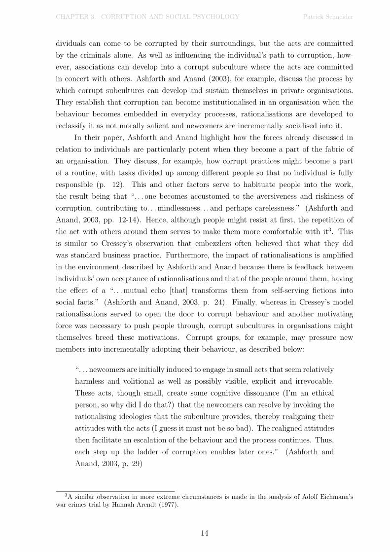
dividuals can come to be corrupted by their surroundings, but the acts are committed
by the criminals alone. As well as influencing the individual’s path to corruption, how-
ever, associations can develop into a corrupt subculture where the acts are committed
in concert with others. Ashforth and Anand (2003), for example, discuss the process by
which corrupt subcultures can develop and sustain themselves in private organisations.
They establish that corruption can become institutionalised in an organisation when the
behaviour becomes embedded in everyday processes, rationalisations are developed to
reclassify it as not morally salient and newcomers are incrementally socialised into it.
In their paper, Ashforth and Anand highlight how the forces already discussed in
relation to individuals are particularly potent when they become a part of the fabric of
an organisation. They discuss, for example, how corrupt practices might become a part
of a routine, with tasks divided up among di↵erent people so that no individual is fully
responsible (p. 12). This and other factors serve to habituate people into the work,
the result being that “. . . one becomes accustomed to the aversiveness and riskiness of
corruption, contributing to. . .mindlessness. . . and perhaps carelessness.” (Ashforth and
Anand, 2003, pp. 12-14). Hence, although people might resist at first, the repetition of
the act with others around them serves to make them more comfortable with it3. This
is similar to Cressey’s observation that embezzlers often believed that what they did
was standard business practice. Furthermore, the impact of rationalisations is amplified
in the environment described by Ashforth and Anand because there is feedback between
individuals’ own acceptance of rationalisations and that of the people around them, having
the e↵ect of a “. . .mutual echo [that] transforms them from self-serving fictions into
social facts.” (Ashforth and Anand, 2003, p. 24). Finally, whereas in Cressey’s model
rationalisations served to open the door to corrupt behaviour and another motivating
force was necessary to push people through, corrupt subcultures in organisations might
themselves breed these motivations. Corrupt groups, for example, may pressure new
members into incrementally adopting their behaviour, as described below:
“. . . newcomers are initially induced to engage in small acts that seem relatively
harmless and volitional as well as possibly visible, explicit and irrevocable.
These acts, though small, create some cognitive dissonance (I’m an ethical
person, so why did I do that?) that the newcomers can resolve by invoking the
rationalising ideologies that the subculture provides, thereby realigning their
attitudes with the acts (I guess it must not be so bad). The realigned attitudes
then facilitate an escalation of the behaviour and the process continues. Thus,
each step up the ladder of corruption enables later ones.” (Ashforth and
Anand, 2003, p. 29)
3A similar observation in more extreme circumstances is made in the analysis of Adolf Eichmann’swar crimes trial by Hannah Arendt (1977).
14

CHAPTER 3. CORRUPTION AND SOCIAL PSYCHOLOGY Patrick Schneider
That corruption is morally frowned upon makes the decision to engage in it significantly
di↵erent from other economic decisions. Not only do individuals need to have the op-
portunity and a positive expected payo↵, but they also need to be able to maintain a
positive self image. If they are unable to achieve this by rationalising corrupt behaviour,
they are unlikely to consider it an option, regardless of its rewards. Developing these
rationalisations and learning how to engage in the behaviour is much easier when an indi-
vidual’s associates also engage in the behaviour. In fact, when an individual is a part of an
organisation that is systematically corrupt they might find conformity to the behaviour
hard to resist. Based on the above discussion, we can see how it is likely that where
organisational cultures of corruption emerge, the behaviour is likely to persist over time
as its commission encourages its repetition. As Ashforth and Anand (2003) note, “. . . [i]n
a real sense, an organization is corrupt today because it was corrupt yesterday.” (p. 14).
If there is enough inertia of this type, the choices of individuals in corrupt organisations
could be completely unresponsive to changes in incentives.
15

Chapter 4
Theoretical Model
In this chapter, I incorporate the key insights discussed in the previous chapter into a
model in which the degree of corruptibility of an o�cial is determined by his own moral
stance as well as by peer e↵ects. The model is based on the class of ‘cognitive dissonance’
models pioneered by Akerlof and Dickens (1982). The particular form adopted here is
from Rabin (1994). In this model, Rabin uses the cognitive dissonance framework to
address decision making with moral concerns (he uses the example of animal rights). In
his formulation, the individual’s decision is sensitive to the moral position of his peers.
This framework for analysing decision making with moral and social constraints is ideally
suited to discuss corruption.
The central variable in the model is the o�cial’s own beliefs about the extent of
corruption that can be considered acceptable, which may be termed his ‘moral stance’.
A key feature of the model is that the o�cial’s moral stance is a↵ected by his perception
of the moral stances of others. Further, his perception of the moral stance of society at
large is disproportionately influenced by the attitudes of agents in his immediate vicinity,
specifically his workplace.
The model yields two principal propositions. First, within a given society with a
uniform structure of incentives and penalties, di↵erent organisations may display di↵erent
levels of corruption in equilibrium. Secondly, these di↵erent equilibrium corruption levels
will persist over time as individuals use past observations of their peers to form their
present beliefs.
This chapter proceeds with a careful description of the behaviour of an o�cial in
this model, emphasising the points of departure from Rabin’s framework. This leads
to the general model, which is then restated using explicit functional forms for the be-
havioural equations. This allows us to obtain closed form solutions for equilibria and
makes comparative static analysis transparent. In the last section the model is extended
to include considerations that are standard in the corruption literature—supervision and
heterogenous agents.
16

CHAPTER 4. THEORETICAL MODEL Patrick Schneider
4.1 Discussion
We imagine that the o�cials, the key actors in our model, work in departments with
given incentive structures and opportunities for corruption. Accepting opportunities for
corruption increases an o�cial’s income and each o�cial chooses the extent to which he
indulges in corrupt behaviour.
O�cials have personal morals that delineate acceptable from unacceptable behaviour
(for example, an o�cial might believe stealing money from a drug dealer is OK but taking
a bribe to let him escape indictment is not). If an o�cial behaves in a way that is
unacceptable by his own moral standards, there is a ‘cognitive dissonance’ between his
judgment that the behaviour is unacceptable and his belief that he is a good and nice
person. This dissonance gives him displeasure.
O�cials can also choose to modify their personal morals against which they judge
their own behaviour. Such adjustment might be in the form of the development of ratio-
nalisations (there is no victim, I deserve it, I do so much good that this is OK, etc.) that
justify a change in his standards of acceptable behaviour. Such adjustment of morals to
a more permissive stance is di�cult to achieve and sustain.
How di�cult moral adjustment is depends both on the magnitude of change and
the judgements and behaviour of the people with whom the o�cial interacts closely. It
is harder to make a bigger adjustment, but the adjustment towards a more permissive
personal attitude is easier, ceteris paribus, when the attitudes surrounding him are more
corrupt and permissive. This latter component is the ‘everyone was doing it’ e↵ect. The
model so far is identical to that proposed by Rabin (1994), with corruption substituted
for violation of animal rights.
My model deviates from Rabin’s in the specification of the o�cial’s perception of the
attitudes of the society around him. Each o�cial works in a particular department, and it
is reasonable to assume that he is exposed more to the attitudes and actions of colleagues
in his department than he is to those of agents in the society at large. The attitudinal
norm of the society may reasonably be represented as exogenous to the immediate choices
of an individual o�cial or a specific department. In the extreme case it may be an
explicit moral code that is insensitive to behaviour, as in the case of a religious doctrine
in a theocratic society—an absolute statement of what is right. The e↵ective moral code
within a department, on the other hand, would be significantly more sensitive to—indeed,
shaped by—the attitudes and choices of department o�cials.
In the present model the o�cial’s perception of the attitudes of society—of what is
acceptable or not acceptable—is determined by both the average attitude of society at
large as well as attitudes within the department. The intuition is that, since the o�cial
interacts more often and more closely with others in his department, the latter’s attitudes
may have a greater weight in determining his perception of the degree of corruption that
the society finds acceptable. If these perceptions then a↵ect his own choice of morals
17

CHAPTER 4. THEORETICAL MODEL Patrick Schneider
and subsequent behaviour, it may happen that two otherwise identical o�cials working
in departments that historically have di↵erent cultures regarding corruption might come
to behave in radically di↵erent ways.
In the next section we formalise the behaviour described above and specify the full
model. We then work with a closed-form version of the model to derive the results that
underlie the hypotheses tested in the empirical section of the thesis.
4.2 Model
4.2.1 General form
The economy consists of several departments, indexed by j, each of which employ a
number of o�cials indexed by i. All o�cials earn a common wage w. Each o�cial also
faces opportunities for corruption from which he can earn a maximum additional income
b. We assume that there is a clear ordering of opportunities from 0 to 1, where 0 is least
objectionable and 1 is most objectionable. Each o�cial chooses the extent to which he
indulges in corruption, �ij 2 [0, 1]. His income is then w + �ijb, from which he derives
utility
U(w + �ijb) where U 0 > 0 and U 00 < 0.
Each o�cial also has a moral line that delineates acceptable from unacceptable
behaviour, ij 2 [0, 1]. If an o�cial indulges in behaviour that is unacceptable by his
own moral standards (i.e. if �ij > ij), he experiences displeasurable cognitive dissonance
thus:
D(�ij � ij) where D0 > 0 and D00 > 0. (4.1)
In addition, the o�cial may also make a positive gain (cognitive ‘resonance’) if his be-
haviour exceeds his own moral standards.
O�cials can choose their moral standards, but it is costly to maintain a stance that
deviates from one that would arise naturally. Let the standard that arises naturally (to
be explained below) be �̂. If the o�cial wishes to maintain a stance 6= �̂, he incurs a
(psychological) cost
C( , �̂), where C > 0, C > 0, C�̂ < 0 and C �̂ < 0.
The beliefs of those around him matter to the o�cial. Specifically, we assume that
each o�cial wishes to act in accordance with the prevailing norm of his society, � 2 [0, 1].
But the beliefs of his society may not be observable to him, so he must estimate them.
His estimate is based on the average of the beliefs of those in his department, ✓j =P
i ij
Nj
and an explicit society-wide moral code that may be unrelated to behaviour, �. So the
18

CHAPTER 4. THEORETICAL MODEL Patrick Schneider
o�cials in department j perceive the moral stance of society to be
�̂j = �̂(�, ✓j). (4.2)
Thus the ‘natural stance’ of o�cial i in department j is �̂j, and he incurs cost C( ij, �̂j)
if he wishes to maintain a moral stance C( ij) that deviates from this.
Each o�cial’s utility is derived by combining the components discussed above as
follows:
Vij(�ij, ij) = U(w + �ijb)�D(�ij � ij)� C( ij, �̂j) (4.3)
Optimisation
Each o�cial solves his problem by optimising this objective function, with his perceptions
of the beliefs of those around him (�̂) taken as given. His optimal choice, as a function of
his perceptions and a vector a of parameters which include w and b, is defined by:
(�⇤ij(a, �̂j), ⇤ij(a, �̂j)) = arg max
�ij , ij
U(w + �ijb)�D(�ij � ij)� C( ij, �̂j) (4.4)
The optimal choice is found by setting first order conditions with respect to the choice
variables equal to zero. Hence �⇤ij and ⇤ij satisfy:
bU 0(w + �⇤ijb) = D0(�⇤ij � ⇤ij) (4.5)
D0(�⇤ij � ⇤ij) = C ( ⇤
ij, �̂j)
That is, the o�cial’s optimal choice of personal moral and corruption levels is found where
the marginal benefit of more corruption is equal to the marginal cost of the dissonance it
would cause, and where the marginal dissonance benefit of raising his moral line is equal
to the marginal cost of doing so.
Equilibrium
An equilibrium is a state where individual o�cials choose their actions optimally in re-
sponse to their perceptions, and in turn their perceptions are realised and perpetuated.
Note that, by (4.2) all o�cials within each department j, must have the same
perception �̂j, since �̂j is determined by the economy-wide variable � and the department-
level variable ✓j. Thus in equilibrium each o�cial must arrive at the same choice of moral
stance and action (�ij, ij). In turn this implies that the department’s average moral
stance ✓j must be equal to the common value of ij. Thus, for a given set of parameters
a an equilibrium is a pair (�⇤ij(a), ⇤ij(a)) that solves the optimisation problem (4.4) given
(w, b, �̂), and �̂ is determined by (4.2) with ✓j = ⇤ij.
In other words, given a parameter set a ⌘ (w, b,�), an equilibrium is a pair
19

CHAPTER 4. THEORETICAL MODEL Patrick Schneider
(�⇤(a), ⇤(a)) that satisfies
(�⇤(a), ⇤(a)) = arg max�ij , ij
U(w + �ijb)�D(�ij � ij)� C( ij, �̂) (4.6)
�̂ = �̂(�, ⇤(a)) (4.7)
Note that this defines a partial equilibrium for the department. A general equilibrium for
the economy would potentially endogenise the society-wide standard �, which I have left
exogenous. This point is revisited below.
4.2.2 Closed form
In this following section, I use explicit functions and obtain closed form solutions for the
model. The money utility function is defined thus:
U(w + �ijb) = w + �ijb (4.8)
Here I have defined a linear money utility function. Such definition does not satisfy the
shape described earlier but is necessary for a unique solution1. Utility is increasing in the
base wage, corruption level and available bribes. The dissonance function is defined thus:
D(�ij � ij) = x(1 + �ij � ij)2 � x (4.9)
Where x is a parameter that scales the dissonance relative to the money utility function
(U). Note that � and take values in the interval [0, 1] hence � � has range [�1, 1].
On this interval D(.) satisfies the restrictions imposed in (4.1). This dissonance function
describes the psychological cost felt from behaving in a way that is at odds with personal
morals. With this function, o�cials who act exactly as their morals allow (�ij = ij) will
experience no dissonance; if they behave in a way that their morals prohibit (�ij > ij),
they experience dissonance that subtracts from utility; and if they are better behaved
than their morals allow (�ij < ij), this adds to utility.2 The moral adjustment cost
function is defined thus:
C( ij, �̂) = z
✓ ij
�̂
◆2
(4.10)
Where z is a parameter that scales the moral adjustment cost relative to the money utility
function (U). Again,the function satisfies the shape restrictions outlined earlier. This
cost function describes the social disutility felt from holding and maintaining permissive
morals, this cost is exacerbated if personal morals are at odds (in either direction) with
1Alternative forms such as log(w + �ijb) yield multiple optimal corruption levels for o�cials who haveset morals. My interest here is in the e↵ect of social interactions on choices, which is not a↵ected by thesimplification.
2These properties hold within the possible range of �1 �ij � ij 1.
20

CHAPTER 4. THEORETICAL MODEL Patrick Schneider
what the o�cial perceives to be normal. That is, it is just as costly for an o�cial to
hold morals that are relatively higher than his perception of his peers’ as it is to hold
morals that are relatively lower—conformity is the easier path. Rabin (1994) uses a
similar functional form. He conceptualises this cost as something that is incurred at
dinner parties—people are required to make statements about their views; those whose
views are di↵erent from normal will experience discomfort, regardless of whether they are
stricter or more permissive than their peers.3
Finally, since agents are homogenous, the department’s average moral level is equal
to a representative agent’s decision, by definition ✓j =P
i ij
Nj= ij. Hence, in equilibrium
�̂ must satisfy �̂ = �̂(�, ij).
Optimisation
Using the defined functional form for the objective function, the first order conditions can
be found as in (4.5), and the optimal choice set for the o�cial derived:
b = 2x(1 + �⇤ij � ⇤ij) (4.11)
2x(1 + �⇤ij � ⇤ij) = 2z
⇤ij
�̂2(4.12)
Substituting 4.11 into 4.12 yields the optimal personal moral level in response to percep-
tions and parameters:
⇤ij =
b
2z�̂2 (4.13)
Substituting 4.13 into 4.11 yields the optimal corruption level in response to perceptions
and parameters:
�⇤ij =b
2z�̂2 +
b
2x� 1 (4.14)
Hence, for a given set of parameters (w, b, z, x) and perceptions �̂, there is a single optimal
choice set available to the o�cial:
⇣�⇤ij(a, �̂j),
⇤ij(a, �̂j)
⌘=
✓b
2z�̂2 +
b
2x� 1,
b
2z�̂2
◆(4.15)
This choice set has the expected properties that personal morality and corruption levels
are increasing with perceptions of society at large,@ ⇤ij@�̂
,@�⇤ij@�̂
> 0, decreasing with the
psychic costs of maintaining morals,@ ⇤ij@z
,@�⇤ij@z
< 0, and increasing with the magnitude
of the bribe opportunity,@ ⇤ij@b
,@�⇤ij@b
> 0. Also, personal corruption is decreasing in the
3The intricacies of conformity are discussed in Bernheim (1994), which proposes a model where peoplederive status from public perceptions of their personal predispositions (similar to our personal moral linehere).
21

CHAPTER 4. THEORETICAL MODEL Patrick Schneider
psychic cost of cognitive dissonance,@�⇤ij@x
< 0. It should be noted that for a fixed available
bribe, the optimal personal corruption level may be either above or below that which
is allowed by personal morals, depending on how strong the psychic cost of dissonance
is. If an o�cial is particularly susceptible (where b2x
< 1), he will benefit from setting a
high moral line but by being less corrupt than it permits (�⇤ij < ⇤ij). Conversely, o�cials
who are less susceptible will optimally behave in ways their own morals do not readily
condone.
Equilibrium
To determine equilibria, we need to explicitly specify the perceptions of the o�cials. I will
consider three cases. The first is where all o�cials perfectly observe the morals of those
within their department, but do not observe morals of agents outside, so that �̂ = ✓j. The
second is where o�cials observe some fixed moral level that is unrelated to people’s actual
choices, i.e., �̂ = � where � is exogenously determined. An example of this is a society
where ‘acceptable’ morals are specified by religious dogma. The third is where o�cials
observe some combination of these, such that �̂ = ↵� + (1 � ↵)✓j where ↵ is the weight
given to the exogenous moral line.4 By the homogeneity of o�cials it follows that, in
equilibrium, we will have ij equal across all o�cials i in department j. By the definition
of ✓j and the assumption of homogeneity, it follows that in all cases we will have ✓j = ij
in equilibrium.
Case 1. Substituting the perceptions in the first case into 4.13 yields the following interior
equilibrium5:
⇤ij =
2z
b(4.16)
Hence, when o�cials perfectly observe those around them, the average moral level in a
department will settle at this single point. Furthermore, as all departments are the same,
each department (and therefore society as a whole) will settle at this equilibrium moral
level. The corresponding equilibrium corruption level where o�cials perfectly perceive
their peers is
�⇤ij =2z
b+
b
2x� 1.
Case 2. Substituting the perceptions in the second case into 4.13 yields the following
equilibrium moral level:
⇤ij =
b
2z�2 (4.17)
4Note that the first two cases correspond to setting ↵ = 0 and ↵ = 1 respectively.5There is also a corner solution ( ⇤ij = 0) that satisfies the condition.
22

CHAPTER 4. THEORETICAL MODEL Patrick Schneider
Hence, when o�cials look solely to some exogenously set moral line (the ‘dogmatic line’),
there is a single equilibrium response as in the case with perfect observation. It is inter-
esting to note that the response to the dogmatic line does not necessarily conform to it.
In fact, the equilibrium moral level will only be equal to the dogmatic line in the case
where � = 2zb
(the equilibrium without the dogmatic line). If the dogmatic line is lower
than this level (less permissive), society will settle at a more permissive level than dogma
dictates. Conversely, if the dogmatic line is higher than this level (more permissive), then
society will settle at a more puritanical level. The corresponding equilibrium corruption
level where o�cials perceive only the dogmatic line is
�⇤ij =b
2z�̂2 +
b
2x� 1.
Case 3. Substituting the perceptions in the third case into 4.13 yields the following:
⇤ij =
b
2z(↵�+ (1� ↵) ⇤
ij)2 (4.18)
Solving for ij, using the quadratic formula, we find the possible equilibrium moral levels
are:
⇤ij =
zb� ↵�(1� ↵) ±
q�↵�(1� ↵)� z
b
�2 � (1� ↵)2 · ↵2�2
(1� ↵)2(4.19)
This yields real solutions if the discriminant is positive, which requires zb
> 2(1 � ↵)↵�.
Note that (1�↵)↵� < 14 since ↵ 2 [0, 1] and � 2 [0, 1]. Hence a su�cient condition for ⇤
to have two real roots is b < 2z. If this condition is satisfied and o�cials’ perception of
prevailing morality is a convex combination of their peers’ morality and that of the wider
society, there are two equilibria.
If the maximum bribe level b is too high or the cost of moral adjustment z is too low,
there is no equilibrium. If the parameter values are such that two equilibria exist, these
specify the morals to which o�cials conform at the department level. Clearly, however,
di↵erent departments can conform to di↵erent equilibria in the same society with the
same overarching code �.
I have not attempted to derive a general equilibrium for the entire society. However,
it can be easily seen that the model can be extended by specifying that � should be some
function of the ✓js across di↵erent departments j. However � is determined, the result
that is relevant to this thesis is that in equilibrium di↵erent departments can persist with
di↵erent levels of corruption, which is the possibility explored further in the empirical
analysis.
These results are a consequence of the chosen functional form—specifically the
square on the denominator of the cost function. They show that the cognitive dissonance
mechanism with incomplete perception of the morals of society can produce multiple equi-
23

CHAPTER 4. THEORETICAL MODEL Patrick Schneider
libria at the department level. With more complex functional forms the model will yield
a larger number of departmental equilibria that can coexist in the same economy. This
finding gives rise to the following hypothesis and implication:
Hypothesis 1. A government department’s organisational culture a↵ects its o�cials’
perceptions of what moral line is acceptable, which in turn a↵ects where they set their own
moral line and how they behave. When their perception of acceptable morality gives weight
to both their peers and an economy-wide standard, di↵erent departments may endogenously
settle at di↵erent equilibrium levels of corruption.
Implication 1A. Departments with identical incentive structures but di↵erent cultures
can exhibit di↵erent levels of corruption.
Furthermore, assuming o�cials’ perceptions of their peers are based on what they observed
of their colleagues in the past, we have a further hypothesis and implication:
Hypothesis 2. The feedback between the perceptions and decisions of o�cials within a
department will cause those perceptions to be realised in future periods. The department’s
culture can therefore endogenously persist over time.
Implication 2A. Departments with identical incentive structures but di↵erent cultures
can exhibit di↵erent levels of corruption persistently over time.
Testing implications 1A and 2A is the focus of the empirical sections.
4.2.3 Extensions
The model presented so far was simplified to elucidate how the cognitive dissonance
mechanism might work. In the following, I introduce extensions to account for supervision
and heterogenous agents that make the model more comparable to standard corruption
models.
Supervision
The first extension is to introduce supervision. We do this by imagining that some external
body conducts reviews of o�cials’ work, but is unable to observe everything and so only
catches corrupt behaviour with some probability, p, i.e. a corrupt o�cial will be caught
with probability p. If an o�cial is caught, we assume he is fined an amount equal to
his wages and any corrupt income. Hence, an o�cial’s expected money earnings are
(1� p)(x + �ijb). It is clear here that the e↵ect of introducing this probability of capture
reduces the marginal benefit of corruption. Consider, for example, the functional forms
used in the previous section. With this extension made to the objective function, the first
24

CHAPTER 4. THEORETICAL MODEL Patrick Schneider
order conditions in the o�cial’s optimisation problem are altered to:
(1� p)b = 2x(1 + �⇤ij � ⇤ij) (4.20)
2x(1 + �⇤ij � ⇤ij) = 2z
⇤ij
�̂2(4.21)
These yield the optimal choice set:
⇣�⇤ij(a, �̂j),
⇤ij(a, �̂j)
⌘=
✓(1� p)
b
2z�̂2 +
b
2x� 1
�, (1� p)
b
2z�̂2
◆(4.22)
Hence, with supervision, the o�cial’s optimal choice is scaled down by the likelihood he
will get to keep his proceeds. Similarly, the equilibria are scaled by this introduction but
their existence is una↵ected.
So far we have treated supervision as an exogenous parameter. It is perhaps more
realistic to assume that the extent of supervision will be related to society’s opinion of
corruption—hence p = p(�) where p(1) = 0, p0(�) < 0 and p(0) = 1. The optimising
o�cial will hence have to take this into account. Recall, however, that a key feature of this
discussion is that the o�cial’s perception of broader society is based on his observation
of his department colleagues and the dogmatic line. Hence, although in reality p = p(�),
the o�cial can only estimate the probability he will be caught—hence p̂ = p(�̂). Suppose
the particular shape of the supervision function is p(·) = 1��. Hence, we can restate the
o�cial’s first order conditions as follows:
�̂b = 2x(1 + �⇤ij � ⇤ij) (4.23)
2x(1 + �⇤ij � ⇤ij) = 2z
⇤ij
�̂2(4.24)
With these conditions, the o�cial still has a single best response to his perceptions:
⇣�⇤ij(a, �̂j),
⇤ij(a, �̂j)
⌘=
✓b
2z�̂3 +
b
2x� 1,
b
2z�̂3
◆(4.25)
The determination of equilibria is slightly altered although their existence still holds.
Figure 4.1 compares the equilibrium levels of ⇤ that arise with and without supervision
for particular values of the parameters (↵ = 0.3, b = 8, � = 0.25 and z = 1). The blue
curve tracks the marginal cost or moral adjustment function with explicit perceptions
(�̂ = ↵� + (1 � ↵) ij) as it varies with personal morals. The yellow and red curves
track the marginal benefit of corruption as it varies with personal morals for the cases
with and without supervision, respectively. The intersections of the latter curves with the
former show where the equilibrium levels of personal morals are. As the figure shows, the
introduction of supervision alters o�cials’ decisions. However, even when supervision is
endogenous, Implications 1A and 2A are not a↵ected.
25

CHAPTER 4. THEORETICAL MODEL Patrick Schneider
Figure 4.1: Equilibrium ⇤ with and without supervision
0.2 0.4 0.6 0.8 1.0y
2
4
6
8
Heterogenous agents
The second extension is to introduce heterogenous o�cials. We do this by imagining
di↵erent ‘types’ of o�cials. As discussed in Chapter 2, this has been done before in
models that include corruptible and incorruptible agents. Here I assume that the two
types di↵er in their susceptibility to the cost of adjusting their morals; i.e. high types6
(z = zH) experience more displeasure than low types (z = zL) for given perceptions
and personal morals. The result is that the two types respond di↵erently to the same
perceptions
⇤H =
b
2zH
�̂2 (4.26)
⇤L =
b
2zL
�̂2 (4.27)
Hence, faced with the same perceptions of what is acceptable, high types will choose a
less permissive personal moral stance than low types. From this we find that the two
responses to the same perceptions result in a relationship between the two such that:
⇤H =
zL
zH
⇤L (4.28)
If we now assume that these types occur in society in given proportions—say a fraction q 2[0, 1] are high types—and that departments all share the same mix of types, perceptions
in equilibrium are formed thus:
�̂ = ↵�+ (1� ↵)(q ⇤H + (1� q) ⇤
L) (4.29)
6As in high moral ground.
26

CHAPTER 4. THEORETICAL MODEL Patrick Schneider
Substituting 4.28 and 4.29 into 4.26 and 4.27 will thus yield the equilibrium moral choices
for high and low types respectively. For example, if we perform the operations for low
types:
�̂ = ↵�+ (1� ↵)
✓qzL
zH
⇤L + (1� q) ⇤
L
◆
�̂ = ↵�+ (1� ↵)m ⇤L (4.30)
Where m =⇣q zL
zH+ (1� q)
⌘2 (0, 1). Substituting this into the expression for the o�-
cial’s optimal moral line (4.27), and solving using the quadratic formula yields the equi-
librium moral line for low types:
⇤⇤L =
zb� ↵�m(1� ↵) ±
q�↵�m(1� ↵)� z
b
�2 � (m(1� ↵) · ↵�)2
(m(1� ↵))2 (4.31)
Hence, as in the case where we assumed homogenous agents, there are two equilibria for
low types when their perceptions of acceptability depends on both their peers and the
dogmatic line. High types will also have two equilibrium moral lines. These will be equal
to the low types’ equilibria scaled down by zL
zH.
This result di↵ers from that with homogenous agents in that with homogeneous
agents, everyone in the department acted in the same way and based their actions on the
departmental average that was equal to the common behaviour. In the present case agents
observe two types of behaviour and act based on the weighted average of those. However,
this still yields multiple equilibria. The di↵erence is that in equilibrium, there are two
responses within a department to the same perceptions—high types are less corrupt than
the average while low types are more corrupt.
It is interesting to note that the multiple equilibria remain even if all departments
have the same mix of high and low types. We could easily see how two departments might
end up with di↵erent cultures if they are populated by entirely high and entirely low types,
respectively. The result found here, however, occurs even holding the mix constant across
departments. Hence, from the analysis in the previous sections, we could say that two
departments with identical incentive structures could exhibit very di↵erent patterns of
corrupt behaviour. We can now add the observation that even if these departments are
populated by o�cials with the same mix of predilections for immoral behaviour, they
might still exhibit di↵erent patterns—and if they did have a di↵erent mix, we would
expect the di↵erence in their patterns to be greater still.
The model shows that o�cials’ perceptions of what is morally acceptable a↵ects their
decisions such that the average behaviour in a department will settle on one of a number
of equilibria. Which equilibrium a department settles on is dependent on its history. In
contrast with previous models, di↵erent levels of corruption are not just an artefact of
27

CHAPTER 4. THEORETICAL MODEL Patrick Schneider
di↵erent incentive structures or supervision mechanisms; nor are they solely a function of
the personalities of the o�cials currently in the department. These results prompt us to
expect that observations of corruption in real world government departments will show
noisy variation (Implication 1A) and persistence over time (Implication 2A).
28

Chapter 5
Data
The remainder of this thesis is concerned with analysing the available data on corruption,
and testing the implications of the theoretical model. I will use the results found in
the comprehensive survey article by Treisman (2007) as the baseline for identifying the
relevant variables to use as controls and significant correlates. My contributions to this
literature are in using updated and department level data, and testing the implications
of a new model of corruption. I am unaware of any study that has used the department
level data before.
This chapter outlines the data that will be used in the analysis, with particular
attention given to the data on corruption. Chapter 6 outlines the empirical strategy that
will be used to test Implications 1A and 2A from the theory and Chapter 7 presents
results.
5.1 Corruption Data
Corruption is di�cult to measure. Because it is an illicit activity, there are no revealed
data available and statistical analysis must rely on stated survey data. These are avail-
able in two forms—perception indices (including Transparency International’s Corruption
Perception Index (CPI) and the World Bank’s Control of Corruption Index (CCI)) and
experience indices (Including Transparency International’s Global Corruption Barometer
(GCB) and the World Bank’s Enterprise Survey (ES)). Most of these indices are published
at the country level. The disaggregated GCB and ES results are, however, available at
the department level as well.
5.1.1 Country level perception indices
Perception indices are constructed using a standard methodology. An organisation with a
network of experts on di↵erent countries asks these experts to rate their country based on
their perception of that country’s level of corruption, or the extent to which questionable
payments are a regular part of doing business. The scores are averaged and transformed
and countries ranked based on the result.
29

CHAPTER 5. DATA Patrick Schneider
Recently, the indices that are used in empirical analysis, such as the CPI and CCI,
are not primary indices but rather aggregations of the results of multiple surveys that
have the structure outlined above. This enhances the number of observations per country
(a significant shortcoming of the earlier surveys) and has also broadened the scope of
interviewees somewhat beyond ‘experts’. The CPI score ranges from one to ten where
higher numbers denote the absence of corruption. The CCI score is a standardised score of
deviations from the average, ranging from approximately �2.5 to 2.5 with higher numbers
denoting the absence of corruption. Summary statistics are reported in Table 5.1.
Perception indices of corruption tend to show similar results. Figure 5.1 shows a
scatter plot of the CPI and CCI results. In this plot, lower numbers indicate more cor-
ruption, so the observations in the south-west corner are for the countries perceived to be
most corrupt and those in the north-east are those perceived to be least corrupt. The vis-
ible linear trend clearly shows the correlation between the two sources (also see Table 5.2).
Figure 5.1
-2-1
01
2C
CI 2
009
0 2 4 6 8 10CPI 2009
Comparison of Perception Indices
Perception indices are fraught with problems, outlined by Treisman (2007), You
and Khagram (2005) and Fisman and Gatti (2002). For example, the experts or others
surveyed may have no actual experience of corruption and so may rely on their recall of
stories they have heard, making them subject to the availability heuristic1. Furthermore,
1Where, when faced with uncertainty, “...people assess the frequency of a class or the probability
30

CHAPTER 5. DATA Patrick Schneider
Table 5.1: Descriptive statistics for corruption measures
Variable n Mean S.D.CPI10 178 4.01 2.09CCI09 204 �0.01 1.00GCB10 83 23.65 21.49
given that the indices are aggregations of others, and that these were ratings out of ten,
their magnitude is not directly interpretable—what is the di↵erence between a seven and
an eight?
These indices have served as the corruption data for most of the empirical analyses,
likely because they have been in existence and improving in quality for many years.
Another major advantage over experience based indices is that they tend to cover more
countries (in 2008, the CPI had 180 observations versus the GCB’s 65). However, the
coverage of experience based indices has been improving over recent years, and their last
release makes them a viable alternative.
5.1.2 Country level experience indices
Transparency International’s GCB presents survey results (summary stats are reported
in Table 5.1) about individual level experiences of bribery in di↵erent countries. There
are typically 1000 respondents per country and the total number of countries covered
has increased to 85 in the 2010 release (up from 65 in 2008). Respondents are asked if
they, or a member of their household, have had contact in the last twelve months with
any of nine government departments2. Those who report contact are asked a follow up
question of whether they, or a member of their household, have paid a bribe to that
department (Transparency International, 2010, pp. 38-39). Country scores are obtained
by reporting the proportion of respondents who reported paying a bribe to at least one
of these departments. Hence, country scores (GCBi) fall somewhere in the range:
max{ni1, ni2, . . . , nij}Ni
GCBi P
j nij
Ni
where nij denotes the number of people in country i who said they had bribed department
j and Ni is the total number who took the survey.
The results from the GCB country scores do not match those of the perception
indices nearly as well as the latter type do with each other. Consider Figure 5.2, which
plots the GCB country scores on top of Figure 5.1. As with the earlier figure, the bottom
south-west shows the most corrupt and the north-east the least corrupt countries. The
of an event by the ease with which instances or occurrences can be brought to mind...” (Tversky andKahneman, 1974, p. 1127)
2Education system, Judiciary/Judicial System, Medical Services, Police, Registry & Permit Services,Utilities, Tax Revenue, Land Services and Customs
31

CHAPTER 5. DATA Patrick Schneider
Figure 5.2
020
4060
8010
0G
CB
2010
-2-1
01
2C
CI 2
009
0 2 4 6 8 10CPI 2009
CCI 2009 GCB 2010
Comparison of Experience and Perception Indices
figure shows that countries with low levels of expert perceived corruption (6-10) actually
do have low levels of experienced corruption. However, in countries with high perceived
corruption (0-5), there is significant variation in experiences. This can also be seen in
Table 5.2 which shows the correlations between the di↵erent measures. Those between
perceptions indices are very high (� 95%) and significant, whereas those between percep-
tions and experience indices are much less pronounced ( 72%), although still significant.
5.1.3 Department level experience indices
The empirical work in corruption uses the country level data discussed above. One contri-
bution of this thesis is to further this work by analysing the department level data. These
data are not published in the primary report, but are made available in their raw form on
the Transparency International website3. I manually collected these disaggregated data
for every year they were available—2010, 2009, 2007 and 2006.
I have made two adjustments to the results. First, due to issues concerning the valid-
ity of the data collected from South Africa and Morocco that are raised by Transparency
International (Transparency International, 2010, p. 34), I have excluded observations re-
lating to these two countries. Second, because the bribery questions are conditional (if
3The 2010 release was downloaded from http://www.transparency.org/content/download/57678/
922770/Tabulations+by+country.zip accessed July 2011
32

CHAPTER 5. DATA Patrick Schneider
Table 5.2: Correlation between country level corruption indices
CPI10 CPI05 CCI09 CCI05 GCB10 GCB05CPI10 1n 178
CPI05 0.97 1n 156 160
CCI09 0.98 0.95 1n 177 160 204
CCI05 0.95 0.96 0.97 1n 176 159 199 199
GCB10 �0.66 �0.66 �0.68 �0.72 1n 81 80 83 83 83
GCB05 �0.66 �0.64 �0.67 �0.71 �0.81 1n 68 66 68 68 57 68
Note: All correlations are significant at the 1% level.
you had contact, did you bribe?), some observations are based on very few responses.
In South Korea, for example, only 24 respondents out of 1500 reported contact with the
judiciary or judicial services and of those, two reported paying a bribe. Hence, in order
to increase validity of the data, observations based on a small number of respondents
were coded as missing values. This biases against departments which have low levels of
contact—particularly customs. As such, the threshold for contact was set at 50 respon-
dents, which is low enough to exclude results based on very few observations but high
enough to allow variation in the customs figures (23 out of 85 observations are excluded).
Another source of disaggregated experience data is the World Bank’s Enterprise Sur-
vey (ES). This survey presents, among many other indicators, responses about firm level
experiences of bribery in di↵erent countries, with firms sampled from the manufacturing
and service sectors. The number of respondents per country in the 2009 survey is 485 on
average, but ranges from less than 100 to over 4000. Much like the structure of the GCB,
the survey asks if the respondents’ firm has had contact with the government over the last
year for a variety of purposes4. Those who report contact are asked a follow up question
of whether a gift or informal payment was expected or requested. The proportion who
answer positively are recorded and the results made publicly available.
As with any survey, the veracity of responses to the GCB and ES can be questioned.
Respondents had answered multiple questions including some relating to their opinions of
corruption and government action against it before answering the questions of interest to
us, which may have tainted their recall. Furthermore, given the generally illegal nature of
corruption, it is possible some respondents may not have wished to answer truthfully. In
4Those focused on in this analysis are—Operating Licence, Import Licence, Construction Permit,Electricity Connection, Phone Connection and Water Connection
33

CHAPTER 5. DATA Patrick Schneider
Table 5.3: Department level GCB 2010 (No bribe)
Department n Mean S.D.Education 83 0.86 0.15Judiciary 78 0.79 0.19Medical 83 0.84 0.14Police 82 0.74 0.24Registry 83 0.82 0.17Utilities 83 0.89 0.13Tax 81 0.86 0.16Land 77 0.82 0.18Customs 53 0.74 0.24
an attempt to overcome this constraint, Transparency International and the World Bank
assure anonymity and deliberately broaden the question to include the experiences of
members of respondents’ household, to allow for personal deniability. Johann Lambsdor↵,
who established Transparency International, suggests one further way to correct for this
is by using the proportion of respondents answering ‘no’ to the bribery question as the
interest variable instead of ‘yes’5. This strategy captures the ambiguous ‘don’t know’
responses, which he finds closely related to corruption levels. Treisman (2007) uses this
strategy and finds it does not significantly alter his results (p. 239) and I use it in the
tests in Chapter 7. Summary statistics for 2010 are reported in Table 5.3.
5.2 Other Data
The variables used to control for known correlates of corruption are based on the dataset
used in Treisman (2007) and include economic, political and institutional factors as well
as historical controls6. The particular variables were chosen from the multitude used in
Treisman’s paper for their jointly high predictive power of corruption (Treisman, 2007,
pp. 233-44, regression no. 7). Tresiman’s dataset is from 2005; I updated the values of
the key variables from the sources named by Treisman where possible. Where more recent
data was not available from Treisman’s source but an alternative was available, I opted
to use the more recent alternative. In some cases, this means the nature of the data is
slightly altered so my results are not directly comparable to Treisman’s.
5.2.1 Variables of interest
Summary statistics of the independent variables are reported in Table 5.4. The economic
variables are the log of GDP per capita in purchasing power parity adjusted terms from
2009 and fuel exports as a proportion of total merchandise exports from 2009. Both were
5A note by Lambsdor↵ on this strategy can be found at http://www.transparency.org/policy_
research/surveys_indices/gcb/2005 accessed 05/09/20116The structure of this section owes a debt of gratitude to Westling (2011)
34
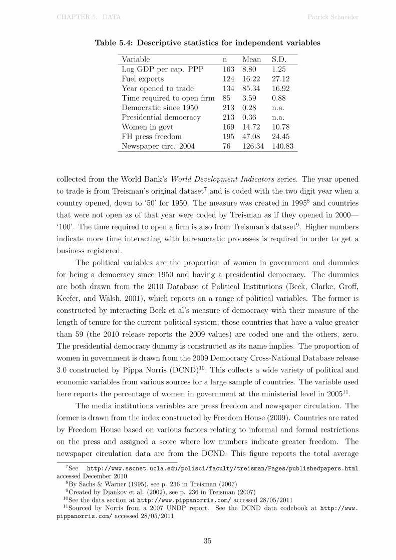
CHAPTER 5. DATA Patrick Schneider
Table 5.4: Descriptive statistics for independent variables
Variable n Mean S.D.Log GDP per cap. PPP 163 8.80 1.25Fuel exports 124 16.22 27.12Year opened to trade 134 85.34 16.92Time required to open firm 85 3.59 0.88Democratic since 1950 213 0.28 n.a.Presidential democracy 213 0.36 n.a.Women in govt 169 14.72 10.78FH press freedom 195 47.08 24.45Newspaper circ. 2004 76 126.34 140.83
collected from the World Bank’s World Development Indicators series. The year opened
to trade is from Treisman’s original dataset7 and is coded with the two digit year when a
country opened, down to ‘50’ for 1950. The measure was created in 19958 and countries
that were not open as of that year were coded by Treisman as if they opened in 2000—
‘100’. The time required to open a firm is also from Treisman’s dataset9. Higher numbers
indicate more time interacting with bureaucratic processes is required in order to get a
business registered.
The political variables are the proportion of women in government and dummies
for being a democracy since 1950 and having a presidential democracy. The dummies
are both drawn from the 2010 Database of Political Institutions (Beck, Clarke, Gro↵,
Keefer, and Walsh, 2001), which reports on a range of political variables. The former is
constructed by interacting Beck et al’s measure of democracy with their measure of the
length of tenure for the current political system; those countries that have a value greater
than 59 (the 2010 release reports the 2009 values) are coded one and the others, zero.
The presidential democracy dummy is constructed as its name implies. The proportion of
women in government is drawn from the 2009 Democracy Cross-National Database release
3.0 constructed by Pippa Norris (DCND)10. This collects a wide variety of political and
economic variables from various sources for a large sample of countries. The variable used
here reports the percentage of women in government at the ministerial level in 200511.
The media institutions variables are press freedom and newspaper circulation. The
former is drawn from the index constructed by Freedom House (2009). Countries are rated
by Freedom House based on various factors relating to informal and formal restrictions
on the press and assigned a score where low numbers indicate greater freedom. The
newspaper circulation data are from the DCND. This figure reports the total average
7See http://www.sscnet.ucla.edu/polisci/faculty/treisman/Pages/publishedpapers.html
accessed December 20108By Sachs & Warner (1995), see p. 236 in Treisman (2007)9Created by Djankov et al. (2002), see p. 236 in Treisman (2007)
10See the data section at http://www.pippanorris.com/ accessed 28/05/201111Sourced by Norris from a 2007 UNDP report. See the DCND data codebook at http://www.
pippanorris.com/ accessed 28/05/2011
35
CHAPTER 5. DATA Patrick Schneider
daily newspaper circulation per 1000 inhabitants in 200412.
5.2.2 History controls
Following Treisman (2007), I also use controls for colonial history, legal tradition and
religion. The colonial history controls are dummies for whether a country was a colony of
various powers13 and were collected from the CIA World Factbook14. The legal tradition
controls are dummies for whether a country has a legal system based on various di↵er-
ent traditions15 and were collected from NYU’s Global Development Network Growth
Database16. The religion controls are dummies for whether a particular religion17 is pre-
dominant in a country (e.g. Saudi Arabia is coded ‘1’ for Muslim and ‘0’ for other
options) and were collected from the DCND. The religion control used here di↵ers from
Treisman’s, which is based on proportions subscribing to various religions. This depar-
ture was deemed appropriate as Treisman’s data on religion is from over three decades
ago. Note that these controls are used with France in mind as the base case—that is, a
non-colony with a French legal system and predominantly Catholic population.
5.2.3 Instruments
The models I will describe in the next section which analyse the relationships between
the variables described above have severe endogeneity issues. The relationship between
GDP and corruption is particularly problematic. As discussed in Chapter 2, there are
various theoretical reasons why corruption would itself a↵ect a country’s income, and
empirical evidence supports this. It is hence necessary to account for reverse causa-
tion by instrumenting GDP. Again, I will follow Treisman’s strategy. He considers two
possibilities—1700 income per capita and 1820 income per capita, both sourced from
Maddison’s (2003) historical GDP dataset (see Treisman (2007, p. 226)). The first is a
valid instrument if “. . . one is willing to assume that a country’s per capita income in 1700
a↵ects current corruption. . . only via the e↵ect on subsequent economic development. . . ”
(Treisman, 2007, p. 226). Using 1700 income per capita reduces the available countries
to 22, so Treisman also uses 1820 income per capita, which o↵ers more observations, on
the same grounds as the other measure.
12Sourced by Norris from a 2008 UNESCO report. See the DCND data codebook at http://www.
pippanorris.com/ accessed 28/05/201113Britain, France, Spain/Portugal, USSR, Other or non-colony14See https://www.cia.gov/library/publications/the-world-factbook/index.html accessed
2/03/201115Socialist, German, Scandinavian, British or French16See http://dri.fas.nyu.edu/object/dri.resources.growthdatabase accessed 22/02/201117Protestant, Muslim, Catholic or Other
36

Chapter 6
Empirical Specifications
There are two goals in my empirical analysis. The primary goal is to test the implications
from the theory outlined in Chapter 4. The secondary goal is to explore the departmental
corruption data, which has not been used before in the empirical literature. The pursuit
of these two goals is, of course, complementary.
Pursuit of the secondary goal simply means I will replicate others’ work (with new
data) more fully than otherwise. The result of this is that, as well as testing the im-
plications of the model, I can compare the results to what has come before. In order
to achieve my primary goal, I employ two approaches to testing—one examines within
country variation between departments and one that uses regression analysis to examine
cross country variation. The latter approach involves two models—one that controls for
country and department e↵ects to isolate the noise predicted by Implication 1A and one
that introduces an extra control for departmental history to control for the persistence
predicted by Implication 2A.
Recall that Hypothesis 1 in the theory is that there will be idiosyncratic variation
in corruption across departments, caused by their cultures. Lacking any data on culture
at the department level, I cannot directly test this mechanism. I can, however, test
Implication 1A—that corruption levels are noisy at the department level.
Suppose the Hypothesis 1 were not true, and departmental corruption levels were
only a↵ected by country level factors. In this scenario, we should observe the same
proportion of people paying bribes to each department, or very small di↵erences resulting
from sampling errors. The correlations between the departments in the GCB are reported
in Table 6.1. Although high, they are unsurprisingly far from perfect and we can reject
this alternative now.
One explanation for this within country variation that still does not admit Hy-
pothesis 1 is that di↵erences between departments within countries are caused by some
department e↵ect. That is, some departments might be systematically more corrupt than
others due to the inherently ‘corruptible’ nature of the work that they undertake. For
example, it seems likely that the police, who have contact with criminal activity and
are bestowed with the legitimate use of violence, will generally be more corrupt than an
education department, who do not and are not.
37

CHAPTER 6. EMPIRICAL SPECIFICATIONS Patrick Schneider
Table 6.1: Correlations between GCB departments
Educ. Jud. Med. Pol. Reg. Util. Tax Land Cust.Education 1Judiciary 0.86 1Medical 0.83 0.76 1Police 0.81 0.88 0.74 1Registry 0.81 0.87 0.77 0.89 1Utilities 0.74 0.76 0.67 0.76 0.87 1Tax 0.80 0.83 0.71 0.78 0.87 0.91 1Land 0.81 0.84 0.78 0.83 0.91 0.86 0.90 1Customs 0.80 0.86 0.72 0.87 0.87 0.75 0.83 0.87 1
Hence, now suppose that Hypothesis 1 were still not true, but that departmental cor-
ruption levels were only a↵ected by country level and these, what I will term ‘systematic
department’, e↵ects. In this scenario, there should be very little noise left in departmental
corruption levels, once country and systematic department e↵ects are accounted for. We
can test this alternative hypothesis in two ways—one using the raw department data to
make within country comparisons and the other using it to make cross country compar-
isons, controlling for country and systematic department e↵ects. If these tests show little
noise, we can reject the hypothesis in favour of the alternative.
Another strategy is to focus on Hypothesis 2 from the theory—that the feedback
between decisions and perceptions causes departmental cultures to persist. Implication
2A suggests that the culture of a department today a↵ects its corruption level, and its
culture is born of the culture in the past. We would hence expect a lagged measure of
that department’s corruption to be a strong predictor of its current corruption. Hence,
the final test will be to include this lagged measure in the regressions of departmental
corruption levels. This test is the closest of the three to testing the actual mechanism
proposed in the model.
The following outlines the empirical strategy to be implemented in the next chapter.
To begin, I consider the distribution of the corruption data to be used, and its implications
for testing. I then consider the two approaches employed to test the hypotheses—the
first is the within country comparison and the second is the cross country regressions.
The latter approach involves two di↵erent models that test alternative implications from
the theory against a baseline model informed by the previous literature. It should be
noted that these tests can help us seek evidence supporting the theory, but they do not
necessarily reject alternative models with similar implications.
6.1 Distribution
The department level corruption indices are not normally distributed. Figure 6.1 plots
the kernel densities for the each department in the GCB 2010 and ES 2009 survey results.
38

CHAPTER 6. EMPIRICAL SPECIFICATIONS Patrick Schneider
Both plots show the distributions are strongly positively skewed with right tails of varying
fatness. A skewness and kurtosis test was performed on each series to test for normality.
This test compares the skew of a distribution and the sharpness of its peak and tails
with those expected in a normal distribution (D’Agostino, Belanger, and D’Agostino Jr,
1990). Assuming normality, the probability of observing the data is below 5% for each
series in the GCB except for the police. Similarly, the probability is below 5% for each
of the covered series from ES1. Hence, it is very unlikely these data come from a normal
distribution. This implies that it would be appropriate to use non-parametric tests to
analyse the raw data, as these do not rely on the restrictive normality assumption.
6.2 Tests
6.2.1 Within country comparison—sign test
A sign test can perform within country comparisons of departments without making the
restrictive normality assumption. The sign test is a non-parametric test that performs a
pairwise comparison of two data series and tests the null hypothesis that they are equally
likely to be larger than each other (that the relationship is noisy). Formally, the sign test
takes two series, X and Y , and tests the hypothesis that for a randomly selected pair of
observations (xi, yi), the di↵erence between the observations is equally likely to be positive
or negative. This amounts to calculating zi = yi � xi and examining the distribution of
zi to see if its median is zero (Mendenhall, Wackerly, and Schae↵er, 1990, pp. 674-677).
The sign test assumes that pairs of observations are randomly and independently selected.
The latter assumption is valid as each observation is for a separate country. The former
assumption could be challenged on the basis that there is selection bias in the countries
covered by the surveys. This challenge limits the external validity of any findings from
the test but is unavoidable.
This test is useful for our purposes because it can act as a test for the strength of
systematic department e↵ects on corruption. If we expected departmental corruption to
only be a↵ected by country level and systematic department e↵ects, then the di↵erence
between the level of corruption in two departments within any given country should have
a consistent sign. Consider the example used earlier, where we expect the police to be
more corrupt than the education department. If there were no e↵ects other than country
and systematic department e↵ects, then the di↵erence between police and education cor-
ruption should be positive for every country. If this were observed, the null hypothesis
of the sign test would be rejected in favour of the alternative that the probability of the
experienced police corruption being greater than education is more than 50%.
Performing the sign test on each pair of departments identifies the existence and
direction of dominant systematic relationships. Rejection of the null in a two-tailed test
1The skewness and kurtosis test results are reported in Appendix A.1
39

CHAPTER 6. EMPIRICAL SPECIFICATIONS Patrick Schneider
Figure 6.1
02
46
8D
ensi
ty
0 .2 .4 .6 .81 - % of respondents who did not pay bribe
EducationJudiciaryMedical ServicesPoliceRegistryUtilitiesTaxLandCustoms
kernel = epanechnikov, bandwidth = 0.0422
GCB 2010 - Department Kernel Densities0
.02
.04
.06
Dens
ity
0 20 40 60 80 100% of firms expected to give gifts
Operating LicenceImport LicenceConstruction PermitElectricity ConnectionPhone ConnectionWater Connection
kernel = epanechnikov, bandwidth = 6.5906
ES 2009 - Department Kernel Densities
40

CHAPTER 6. EMPIRICAL SPECIFICATIONS Patrick Schneider
identifies a relationship where a systematic e↵ect dominates, as discussed above; a one-
tailed test can then determine the direction of this relationship. Failure to reject the
null in a two-tailed test identifies either an equal or a noisy relationship. If, upon deeper
investigation of these relationships, we then observe variation in di↵erences (ruling out
the possibility that the departments are identical), we have a preliminary indication that
idiosyncratic e↵ects exist.
6.2.2 Cross country comparison—regressions
Using multiple linear regression allows for stronger tests of the hypothesis using the avail-
able data. As discussed in Chapter 5, I will use the regressions in Treisman (2007) as the
starting point. Treisman tests relationships between corruption and other factors using
OLS regressions of the following form:
corri = �0 + �1Ci + "i (6.1)
Where i indexes country and Ci is the vector of the independent variables and controls
discussed in Chapter 5.
Baseline model
The first step in this analysis is to rerun these regressions using the model in (6.1) to
establish what di↵erence, if any, there is between results found with perceptions and
experience indices. Treisman finds many significant relationships and very high predictive
power (R2 = 0.92 in model (7) pp. 233-234) using perceptions indices but very few
significant relationships when the experience index is used as the dependent (pp. 239-40).
I expect these results to be reproducible with the newer data. This provides a baseline
against which to compare the results of the models to come.
Model 1
The next step is to extend the baseline analysis by disaggregating the corruption expe-
rience data and using the new data as the dependent. The theoretical determinants of
department level corruption are as follows:
corrij = �0 + �1Ci + �Dj + �X⇤ij + uij (6.2)
Where j indexes department, Dj is a dummy variable for each department, controlling
for systematic department e↵ects (the base is the education department) and X⇤ij is the
unobserved idiosyncratic culture e↵ect. If it were not true that the last factor was a de-
terminant of departmental corruption then the following would be an unbiased estimator:
corrij = �0 + �1Ci + �Dj + uij (6.3)
41

CHAPTER 6. EMPIRICAL SPECIFICATIONS Patrick Schneider
Hence, in this step, it is assumed that the hypothesis is false. The dependent variable is
departmental corruption and the independents are the standard country level regressors
and controls as well as controls for systematic department e↵ects. Here, we are interested
in the level of noise remaining in the model after these factors are controlled for. A lower
adjusted R2 indicates more noise and therefore more room for the theory.
Using department level data introduces a new issue. As each country has up to
nine observations, it is unlikely that each observation is independent. This could lead
to violation of the model’s assumption that the data are independently and identically
distributed. If present, this violation biases standard errors. Given this risk, department
level standard errors are adjusted using cluster methods, similar to robust standard errors
but where the weight is unique to the common element (in this case, country) rather than
the observation.
Model 2a
The next step is to recognise that if the hypothesis is true, then not controlling for culture
e↵ects introduces omitted variable bias into the model. Being able to control for culture
e↵ects would thus be helpful for two reasons—it would remove this bias and also provide
a testable estimate of the relationship that the theoretical model proposes. There is no
direct data on the culture within the departments in question, but the data on corruption
in these departments from previous periods might provide a valid proxy (Wooldridge,
2009, pp. 306-12). The logic here is that according to the theory, current culture should
be closely linked to the past culture. If the past culture also causes past corruption (as is
proposed by the theory), then we can use past corruption as a proxy for present culture.
This proxy relationship is expressed formally as follows:
X⇤ij = ↵0 + ↵1corrij,lag + µij (6.4)
Substituting the proxy relationship in (6.4) into the model outlined in (6.2) and rearrang-
ing terms yields:
corrij = (�0 + �↵0) + �1Ci + �Dj + �↵1corrij,lag + vij (6.5)
Where there is a composite error term vij = uij + �µij. Hence, in this final step, the
strength of the relationship between the present and lagged levels of corruption (signif-
icance of the coe�cient on corrij,lag) gives an indication of the role that a department’s
history has to play in its present corruption level. This model is rerun using di↵erent lags
to assess the persistence of the relationship over di↵erent periods of time.
Model 2b
The last step utilises the time dimension of the department level corruption data to rerun
Model 2a with more observations. The department level corruption data are available for
42

CHAPTER 6. EMPIRICAL SPECIFICATIONS Patrick Schneider
the years 2010, 2009, 2007 and 2006. This structure means a pooled-cross section (2010
and 2007) can be analysed with a one year lag. The model estimated in this step is similar
to the model in 6.5, but is formally expressed as follows:
corrijt = (�0 + �↵0) + �1Cit + �2Ci + �Dj + �↵1corrijt�1 + ⇣ijt (6.6)
The di↵erence here is that some country level variables are allowed to vary over time and
we are limited to a lag of one year.
I considered using the time dimension of the data to run other standard time series
models but found that they weren’t appropriate. First di↵erencing, for example, is a
technique aimed at eliminating time persistent but unobservable e↵ects. Although this
is extremely useful in other circumstances, it is precisely these e↵ects we’re interested in
here, so it was not deemed appropriate to exploit the time dimension in ways other than
those already discussed.
Robustness checks
Tests for joint significance of categories of interest variables and functional form misspeci-
fication (RESET) are performed on each of the above regressions. All standard errors are
reported in robust form for country level regressions and clustered form for department
level regressions. All reported regression results use the log transformation of the cor-
ruption (dependent and lag) variables. The department level data are transformed using
the method recommended by Lambsdor↵2, where log corrij = �ln(1.01 � no bribeij); in
other cases, the simple natural log is used where log corri = ln(corri). The level versions
of the models were also run but were generally found to be inappropriate specifications.
2See http://www.transparency.org/policy_research/surveys_indices/gcb/2005 accessed05/09/2011
43

Chapter 7
Results
7.1 Department Level Variation in Corruption
There is evidence for both systematic and idiosyncratic department e↵ects on corruption.
This is confirmed by sign tests1 on the pairwise comparison of each variable in the GCB
and ES results. To see this, refer to Table 7.1, which shows the likely direction of system-
atic department e↵ects. The table was constructed by first conducting a two-tailed sign
test on each pair of departments at the 5% level of significance to see if there was any
indication of a systematic department e↵ect. If the null hypothesis was not rejected, the
cell was coded ‘0’ to indicate no dominant systematic department e↵ect. If the hypothesis
was rejected, a positive one-tailed test was conducted at the 5% level of significance to see
if there was any indication that the column department was systematically more corrupt
than the row department. If the null hypothesis was again rejected, the cell was coded ‘+’
to indicate a systematic department e↵ect where the column department is more corrupt
than the row department. If the null hypothesis was not rejected, the cell was coded ‘�’
to indicate the opposite.
Take, for example, the police department, whose relationships are found in the fourth
column of the GCB table. The series of ‘+’ symbols indicates that, at the 5% level of
significance, the police department is systematically more corrupt than the education,
judiciary, medical, registry, utilities, tax and land departments. The ‘0’ in the last row
indicates no evidence of a systematic relationship with the customs department which,
after further examination, might allow us to identify an idiosyncratic relationship.
7.1.1 Systematic department e↵ects
There is strong evidence that systematic department e↵ects impact the level of corruption
in various departments. This is shown by the wealth of significant relationships identified
by the sign test in both the GCB and ES. Looking at a department’s relative number of
the di↵erent relationships shows some very interesting patterns. From the GCB, a rough
hierarchy of systematic department e↵ects can be found by ranking departments by the
1The p-values of two- and one-tailed tests are reported in Appendix A.2
44

CHAPTER 7. RESULTS Patrick Schneider
number of positive, then neutral and then negative relationships—Police > Customs >
Judiciary > Registry = Land > Medical > Education > Tax > Utilities.
The police and customs appear to be systematically more corrupt than most other
departments, supporting the examples in Chapter 6 and conforming to intuition. At the
other end of the scale, the tax and utilities departments appear to be systematically less
corrupt than most other departments. That the tax department should be systematically
less corrupt than others is surprising. Although governments certainly have a strong
incentive to keep this department clean, anecdotal and case study evidence (for example,
see Klitgaard (1988, pp. 13-51)) leads us to expect tax departments to be fairly corrupt.
One explanation for this result, then, could be that the nature of the tax department’s
work is such that bribes will be paid willingly (e.g. to push through inflated deductions)
rather than extorted by o�cials. Such collusive arrangements are much less likely to be
admitted by survey respondents. This sheds light on one of the limitations of the data—
it is only likely to reflect acts of bribery that respondents feel either angry about or not
personally culpable for. The survey only represents itself as a measure of bribery, but it
is likely that the scope of the activity is even greater than the results suggest.
The same process, but using the ES data now, shows that the construction permit
process appears to be systematically more corrupt than all other departments and the
phone connection process less so than most others. The rough hierarchy of systematic de-
partment e↵ects implied by the ES is—Construction Permits > Electricity Connections >
Water Connections > Operating Licences > Import Licences > Phone Connections.
Table 7.1: Pairwise relationships (column� row) between departmentalcorruption implied by sign test
GCB 2010 Educ. Jud. Med. Pol. Reg. Util. Tax Land Cust.Education + + + + � 0 + +Judiciary � � + 0 � � 0 0Medical � + + 0 � � 0 +Police � � � � � � � 0Registry � 0 0 + � � 0 +Utilities + + + + + 0 + +Tax 0 + + + + 0 + +Land � 0 0 + 0 � � +Customs � 0 � 0 � � � �
ES 2009 Op. Lic. Imp. Lic. Cons. Per. Elec. Con. Pho. Con. Wat. Con.Op. Lic. 0 + 0 0 0Imp. Lic. 0 + + 0 0Cons. Per. � � � � �Elec. Con. 0 � + � 0Pho. Con. 0 0 + + +Wat. Con. 0 0 + 0 �
45

CHAPTER 7. RESULTS Patrick Schneider
7.1.2 Idiosyncratic department e↵ects
There is also strong evidence for idiosyncratic department e↵ects. Each cell coded ‘0’
in Table 7.1 indicates that there is no evidence for a dominant systematic relationship
between the two departments. This means that the two departments are either system-
atically the same or that the relationship is noisy.
In order to determine which alternative is the case, we can simply look at the
distribution of di↵erences. Figure 7.1 maps box plots for each of these relationships.
These show that the relationships do, in fact, exhibit noisy di↵erences. Take, for example,
the plot for the police and customs departments in the GCB. The spread of the whiskers
either side of the zero line shows that in many countries, the police are more corrupt than
the customs department (e.g. Argentina, Bosnia, Latvia, Pakistan, Russian Fed. and
others) and that the opposite is true for many others (e.g. Afghanistan, Kosovo, Lebanon,
FYR Macedonia, USA and others). This idiosyncrasy is evident for each combination of
departments where a dominant systematic e↵ect was not identified. In fact, it is observable
even in combinations where there is a dominant systematic e↵ect (e.g. in Vietnam in
2010, 16% less people reported paying a bribe to the judicial system than the education
department), although not to the same extent.
Analysis of the department level data finds evidence in support of Implication 1A—that
variation in corruption has an idiosyncratic component. This variation is separate from
systematic department e↵ects caused by the corruptible nature of a department’s work.
It is also separate from the scope of the department’s work, as both indices measure
the incidence of bribery conditional on the respondent’s having had contact with the
department. We thus fail to reject Hypothesis 1 from the theory—that departmental
subcultures can sustain di↵erent corruption levels in departments.
7.2 Cross-Country Regression Estimation
In this remainder of this chapter, I present the results from the cross-country regression
models outlined in Chapter 6 with a focus on the GCB department data. My starting
point was to run each of the models in the following section with the full set of Treisman’s
independent variables, as outlined in Chapter 5. However, I found various issues with
these models that a↵ected their interpretation and gave me cause to make modifications.
First, there were very few observations available for the newspaper circulation variable.
Its inclusion in the models tended to render them incapable of producing any meaningful
results as sample sizes were so reduced. It was removed from the set of regressors to
enhance sample size and also on the reasoning that it and the FH Press Freedom mea-
sure should capture similar e↵ects2. Second, although Treisman’s ‘democracy since 1950’
2They have a correlation coe�cient of -0.56, which is significant at standard levels.
46

CHAPTER 7. RESULTS Patrick Schneider
Figure 7.1
-.4-.2
0.2
.4Pe
rcen
t diff
eren
ce
GCB 2010 - Idiosyncratic Corruption Differences
Education - Tax Judiciary - RegistryJudiciary - Land Judiciary - CustomsMedical - Registry Medical - LandPolice - Customs Registry - LandUtilities - Tax
-60
-40
-20
020
40Pe
rcen
tage
poi
nt d
iffer
ence
ES 2009 - Idiosyncratic Corruption Differences
Operating lic. - Import lic. Operating lic. - Electricity con.Operating lic. - Phone con. Operating lic. - Water con.Import lic. - Phone con. Import lic. - Water con.Electricity con. - Water con.
47

CHAPTER 7. RESULTS Patrick Schneider
variable was found to be significant, the models that included it all su↵ered from func-
tional form misspecification. Replacing this variable with a control for the square of the
length that democracy has presided in years reduces this issue. I proceed now through the
Baseline Model, Model 1 and Model 2 with the leaner and modified set of independent
variables.
7.2.1 Baseline model
The first step in the cross-country analysis is to establish the Baseline Model, which is
closely based on one of the models from Treisman (2007). The results reported in Ta-
ble 7.2 show the relationships between the log transformation of country level corruption
measures and our independent variables. Although not an exact reproduction of Treis-
man’s model (logs are used rather than levels and changes to variables have been made
as discussed), the findings are similar.
The estimations that have a perception index as the dependent variable (1 & 2) have
high predictive power (adjusted R2 is 81%) and find various precisely estimated relation-
ships. Higher development, less prominence of fuel exports and shorter waiting times
to open a firm are all significantly correlated with lower levels of perceived corruption.
Greater press freedom and opening to trade earlier are also correlated with lower per-
ceived corruption, although these relationships are not robust to the inclusion of controls
for legal tradition, colonial history and religion (hereafter referred to as ‘the controls’).
In contrast, the estimations that have an experience index as the dependent variable (3
& 4) have lower predictive power (adjusted R2 is 68% when the controls are not included
and 65% when they are) and few precisely estimated relationships. Higher development,
more women in governmental positions and the squared length of democracy are all found
to be correlated with less experience of bribery, although the latter two relationships are
not robust to the inclusion of the controls. The relationships discussed above and the
di↵erences between the results found with perception and experience indices are similar
to those identified by Treisman, as expected.
7.2.2 Model 1
From this point on, the analysis departs from the previous literature by using the de-
partment level data on experiences of bribery as the dependent variable. Estimations
5 & 6, reported in Table 7.3, are a reproduction of the Baseline Model, but use this
new dependent variable. The relationships are comparable to those found in the country
level equivalents (3 & 4) but the predictive power is much lower. This is as expected—
if we found that experiences of department level bribery were well explained solely by
country level factors, that would imply no room for systematic department e↵ects, which
were found in abundance earlier in this chapter, let alone the idiosyncratic culture e↵ects
predicted by Hypothesis 1 in the theory.
48

CHAPTER 7. RESULTS Patrick Schneider
Table 7.2: Country level regressions with logged dependent
1 2 3 4log CPI10 log CPI10 log GCB10 log GCB10
ln GDP per 0.1421⇤⇤⇤ 0.1713⇤⇤⇤ �0.5582⇤⇤⇤ �0.5856⇤⇤⇤cap. PPP (0.0373) (0.0507) (0.1074) (0.2073)
Fuel exports �0.0038⇤⇤⇤ �0.0035⇤⇤⇤ 0.0046 0.0047(0.0011) (0.0012) (0.0034) (0.0040)
Year open �0.0047⇤ �0.0019 0.0034 �0.0036to trade (0.0025) (0.0028) (0.0064) (0.0111)
Time required to �0.0772⇤⇤ �0.1097⇤⇤ 0.0345 0.1255open firm (0.0291) (0.0497) (0.1416) (0.2080)
Presidential �0.0470 0.0111 0.0227 0.1978democracy (0.0666) (0.0708) (0.2773) (0.3269)
FH Press �0.0039⇤ �0.0023 �0.0037 �0.0047freedom (0.0021) (0.0025) (0.0172) (0.0105)
Women in 0.0026 0.0024 �0.0194⇤⇤ �0.0120government (0.0019) (0.0024) (0.0076) (0.0105)
Years democracy 0.0000 0.0000 �0.0001⇤ �0.0001squared (0.0000) (0.0000) (0.0001) (0.0001)
Constant 0.9364⇤ 0.5320 7.9348⇤⇤⇤ 8.0175⇤⇤(0.4764) (0.6429) (1.3861) (2.9449)
History controls no yes no yes
Adjusted R
2 0.81 0.81 0.68 0.64n 72 72 52 52
Notes: Dependent variable measures absence of corruption in 1–2 and presence of corruption in 3–4.White robust adjusted standard errors are reported. Significance of coe�cients is shown by ⇤ wherep < 0.10, ⇤⇤ where p < 0.05 and ⇤⇤⇤ where p < 0.01.
49

CHAPTER 7. RESULTS Patrick Schneider
The next step is to examine the results for Model 1, which are reported in Table 7.3
as estimations 7 & 8. These repeat the baseline specification at the department level, but
include dummies to control for systematic department e↵ects. The department dummies
are highly individually and jointly significant3 and their inclusion improves the predictive
power of the model by six percentage points, both with and without the controls. This
confirms the finding earlier in the chapter that there are strong systematic factors that
a↵ect department level corruption. Although Model 1 has good predictive power4, it
remains less powerful than the Baseline Model using the country level experience index
and there is still significant unexplained variation in reported experiences of bribery.
In this step, we assumed that the hypothesis was not true. That is, we assumed that
country and systematic department e↵ects fully explained department level experiences
of corruption. In Model 1, we have controlled for these e↵ects and found that there is still
a significant amount of noise left in the dependent variable. Model 1 thus leaves room
for other explanations of the level of corruption in departments. The hypothesis that the
idiosyncratic organisational cultures of government departments a↵ects their corruption
levels is one such explanation that is consistent with these results.
7.2.3 Model 2
Implication 2A from the theory states that corruption levels will be persistent over time. If
the decisions of o�cials within a department are based on their perceptions of those around
them and their past experiences, their decisions will settle in a coordinated equilibrium
and the same modes of behaviour will persist over time. In this model, we introduce a lag
of the dependent variable to proxy for the department’s culture, but also to capture this
persistence e↵ect. As outlined in Chapter 6, the coe�cient to this lag tells us the joint
impact of past corruption on present culture and present culture on present corruption.
The results for Model 2a are reported in Table 7.3. Estimations 9 & 10 repeat the
estimations in Model 1 but include the lagged dependent as an explanatory variable. The
new term is very precisely estimated and its impact is highly economically significant—in
estimation 9, a 10% increase in experiences of bribery in the previous period is predicted
to be associated with a 4.1% increase in the present period. The inclusion of this new
term increases the predictive power of the model by 12 percentage points, both with and
without the controls. With the inclusion of this new term, however, previously significant
relationships are no longer found to be so. With such a short lag, this is possibly caused
by the persistence in value of the other variables. Alternatively, there could be too few
observations to have enough variation to establish other relationships.
3F (8, 52) = 9.05 and p = 0.000 for estimation 7 and F (8, 52) = 9.19 and p = 0.000 for estimation 8
4Adjusted R
2 is 53% in estimation 7 and 58% in estimation 8.
50

CH
AP
TE
R7.
RE
SULT
SPatrick
Schneider
Table 7.3: Department level regressions with logged dependent
Baseline Model 1 Model 2a Model 2b5 6 7 8 9 10 11 12
log GCBD10 log GCBD10 log GCBD10 log GCBD10 log GCBD10 log GCBD10 log GCBD10&07 log GCBD10&07log GDP per 0.4469⇤⇤⇤ 0.3495⇤⇤ 0.4482⇤⇤⇤ 0.3526⇤⇤ 0.1838 �0.0457 0.1529⇤ �0.0874cap. PPP (0.0970) (0.1475) (0.0977) (0.1496) (0.1164) (0.1504) (0.0870) (0.1246)
Fuel exports �0.0037 �0.0031 �0.0037 �0.0031 �0.0004 0.0016 �0.0015 0.0016(0.0023) (0.0031) (0.0023) (0.0031) (0.0024) (0.0032) (0.0023) (0.0026)
Year open �0.0026 �0.0036 �0.0022 �0.0033 �0.0035 �0.0113 �0.0084⇤ �0.0179⇤⇤⇤to trade (0.0046) (0.0073) (0.0047) (0.0075) (0.0054) (0.0079) (0.0047) (0.0067)
Time required to 0.0948 0.0988 0.0921 0.1026 0.1170 0.1016 0.1939⇤⇤ 0.2563⇤⇤open firm (0.0710) (0.1119) (0.0707) (0.1142) (0.0902) (0.1127) (0.0820) (0.1146)
Presidential 0.0741 �0.2177 0.0768 �0.2149 0.0912 �0.3078 0.3143⇤ �0.0019democracy (0.2106) (0.2336) (0.2108) (0.2351) (0.2176) (0.2638) (0.1686) (0.2331)
FH Press �0.0017 0.0015 �0.0015 �0.0018 �0.0023 0.0061 �0.0068 0.0019freedom (0.0050) (0.0059) (0.0050) (0.0060) (0.0049) (0.0072) (0.0043) (0.0061)
Women in 0.0123⇤⇤ 0.0005 0.0128⇤⇤ 0.0008 0.0035 �0.0088 0.0036 �0.0085government (0.0059) (0.0056) (0.0059) (0.0058) (0.0081) (0.0076) (0.0064) (0.0072)
Years democracy 0.0001 0.0001 0.0001 0.0001⇤ 0.0001⇤⇤ 0.0001⇤⇤ 0.0001⇤⇤ 0.0001⇤⇤squared (0.0000) (0.0000) (0.0001) (0.0000) (0.0000) (0.0001) (0.0001) (0.0001)
log GCBDt�1 0.4124⇤⇤⇤ 0.4335⇤⇤⇤ 0.4512⇤⇤⇤ 0.4761⇤⇤⇤(0.1051) (0.0928) (0.0908) (0.0810)
Constant �2.2531⇤ �1.0679 �2.0694⇤ �0.9080 �0.6478 2.2801 �0.3237 2.6064(1.1744) (2.0141) (1.1816) (2.0541) (1.2112) (2.0209) (0.9706) (1.7085)
Department controls no no yes yes yes yes yes yesHistory controls no yes no yes no yes no yes
Adjusted R
2 0.47 0.52 0.53 0.58 0.65 0.70 0.68 0.72n 446 446 446 446 324 324 511 511
Notes: Dependent variable measures absence of corruption. Cluster adjusted standard errors are reported. Significance of coe�cients is shown by ⇤ where p < 0.10, ⇤⇤where p < 0.05 and ⇤⇤⇤ where p < 0.01.
51

CHAPTER 7. RESULTS Patrick Schneider
The first of these issues is partly remedied by rerunning the estimations with di↵erent
lags. Results are reported in Table 7.4. The significance of the persistence relationship
is still observed when using 2007 and 2006 observations as lags, although its strength is
somewhat diminished—a 10% increase in experiences of bribery in 2006 is predicted to be
associated with a 3.6% increase in present day experiences. Using these other lags does
bring some of the other relationships back—most notably the log of GDP per capita and
time required to open a firm, although the latter is only precisely estimated when the
2006 lag is used. Unfortunately, the data only go back to 2006, so earlier lags are not
available.
The second of these issues is remedied by utilising the time dimension of the data
in the way outlined in Chapter 6 as Model 2b. The 2010 and 2007 results are pooled and
run in the same way as Model 2a (with a one year lag), results are reported in Table 7.3 as
11 & 12. This method increases the number of observations and improves the predictive
power of the model by a further two to three percentage points. With the greater sample
size, the coe�cient to the lag variable remains precisely estimated as are other factors
such as the year open to trade, time required to open a firm and the square of the length of
democracy. Hence, the persistence of experiences of bribery that is observed in Model 2 is
showing some relationship other than the persistence of the other independent variables.
Interestingly, the relationship found with time required to open a firm in estima-
tions 11 & 12 is in the opposite direction to that expected. Theory tells us that more
bureaucratic choke points (in the form, for example, of the process of registering a busi-
ness) create more opportunity for corruption and, hence, we expect more experiences of
corruption. In contrast to theory, the relationship predicted here is that the longer the
time required to register a business, the less the expected experienced corruption. This
relationship is robust to the inclusion of the controls (in fact the coe�cient grows in
magnitude). This finding contradicts the findings of Treisman and some of my own esti-
mations (1 & 2). One possible explanation for this could be that the corruption inducing
aspects of this variable’s e↵ect are being captured by the lag, and that what is left is the
e↵ect of a more thorough, but less corrupt, government.
In this step, we come closest to testing the actual mechanism in the model. In the-
ory, the present level of corruption is caused by present organisational culture, which is
related to past experiences. An implication of this is that we should observe persistence
in corruption levels within departments. The inclusion of lagged dependents finds strong
evidence of this, albeit over rather short periods of time. The strength of this relationship
is robust to the available lags, strengthened by pooling di↵erent (but adequately dis-
tant) time periods and cannot be explained solely by the persistence of other explanatory
variables.
52

CHAPTER 7. RESULTS Patrick Schneider
Table 7.4: Model 2a results with di↵erent lags
7 13 14log GCBD10 log GCBD10 log GCBD10
Lag year xxxx 2009 2007 2006ln GDP per 0.1838 0.2578⇤⇤ 0.2406⇤⇤⇤cap. PPP (0.1164) (0.1155) (0.0867)
Fuel exports �0.0004 0.0011 0.0017(0.0024) (0.0033) (0.0025)
Year open �0.0035 �0.088 �0.0069to trade (0.0054) (0.0060) (0.0060)
Time required to 0.1170 0.0077 0.1556⇤⇤open firm (0.0902) (0.0824) (0.0786)
Presidential 0.0912 0.0067 0.1826democracy (0.2176) (0.2311) (0.1911)
FH Press �0.0023 0.0043 �0.0036freedom (0.0049) (0.0053) (0.0051)
Women in 0.0035 0.0110 0.0093government (0.0081) (0.0088) (0.0069)
Years democracy 0.0001⇤⇤ �0.0000 0.0001squared (0.0000) (0.0000) (0.0000)
Dept corruption 0.4124⇤⇤⇤ 0.3618⇤⇤⇤ 0.3597⇤⇤⇤in year xxxx (0.1051) (0.0910) (0.1071)
Constant �0.6478 �0.5351 �0.9652(1.211) (1.3291) (1.1525)
Department controls yes yes yesHistory controls no no no
Adjusted R
2 0.65 0.67 0.67n 324 189 279
Notes: Dependent variable measures absence of corruption. Cluster adjusted standard errors are reported.Significance of coe�cients is shown by ⇤ where p < 0.10, ⇤⇤ where p < 0.05 and ⇤⇤⇤ where p < 0.01.
53

CHAPTER 7. RESULTS Patrick Schneider
7.3 Limitations
The empirical tests allow for the implications of the theory. These results should, however,
be carefully interpreted as they are limited in important ways. First, it should be noted
that none of the tests are a direct test of the theory itself. Rather, they test whether
alternatives to the theory are enough to explain observed variation—that is, do country
and systematic department e↵ects alone cause variation in experiences of bribery. Each
test finds that these factors do not fully explain the variation, but this is not to say
that the theory is therefore confirmed. There are various, in fact infinite (Friedman,
1966), alternative explanations for the observed phenomena. Hence, we can only say that
the results fail to rule out our hypothesis. Further research could isolate these di↵erent
explanations for departmental idiosyncrasies. For example, if we had data on the incentive
and supervision structures of the same departments across countries, we would be closer
to being able to isolate the culture e↵ect—although these two factors would arguably be
jointly determined.
By controlling for the persistence of experiences of bribery, Model 2 comes closest
to testing the actual theory; although it, too, does not rule out alternative explanations.
A second limitation of these tests, however, is that the lags used in Model 2 are short.
If corrupt organisational cultures persist over time, we would expect this to be true over
periods much longer than the available data allows us to test. Further research could seek
to find department level measures of incentives, corruption or organisational culture from
the more distant past in order to establish how persistent the behaviour actually is.
A third limitation is that the relationships between the dependent and independent
variables are likely to be highly endogenous. We expect, for example, that corruption
would be jointly determined with economic development and red tape (time to open
a business) and can see that other endogenous relationships are likely. This fact has no
e↵ect on the findings we’re interested in, but it does bias the coe�cients of the explanatory
variables so their interpretation is spurious. An attempt was made to correct for at least
some of this by instrumenting the log of GDP per capita with the log of GDP per capita
in 1820 per Treisman’s paper. Doing so substantially reduces the number of observations
available and gives spurious results that I will not discuss here, although they are reported
in Appendix A.3.
A fourth limitation is the data used to measure corruption itself. As has been dis-
cussed at length, the department level experience data collected by Transparency Inter-
national seek to measure the proportion of people required to pay a bribe to a department
given that they had contact with that department. Due to the illicit nature of bribery,
it is likely that survey respondents have not fully reported their behaviour. Steps were
taken where possible to take this into account (for example, by using ‘no’ responses as
the dependent variable). Even so, it is likely that insofar as the GCB measures anything,
it measures only those bribes that respondents paid resentfully (as suggested by tax de-
54

CHAPTER 7. RESULTS Patrick Schneider
partments’ surprising relative cleanliness). Hence, the relationships discussed in these
tests apply to a small part of the widespread phenomenon that is corruption. The use
and interpretation of these data is therefore limited. However, by using department level
data, which is closer to the predictions of most theoretical models and less processed after
the original survey, it is an improvement on past research and shows new avenues that
can be explored in the future.
55

Chapter 8
Conclusion
This thesis examines how the moral decisions of government o�cials can cumulatively
create organisational subcultures that foster corrupt behaviour. Analysts of criminology
and social psychology argue that rationalisations of and methods for morally deviant
behaviour must be learned from close associations. When these associations occur in the
context of an organisation, patterns of corrupt behaviour can come to be a part of that
organisation with the e↵ect that they become normalised and widespread.
Whereas most economic corruption models focus on structural incentives, my model
takes a di↵erent approach by examining organisational culture. Using a modified version
of the cognitive dissonance model by Rabin (1994), I examine o�cials’ decisions when they
must contend with their own personal morals and also their perceptions of what is normal.
I find that idiosyncratic di↵erences between the average corruption levels of di↵erent
departments can exist, independently of incentives, when o�cials base their perception
of what is a normal moral attitude on a mix of a fixed social norm and the beliefs of
their colleagues. I further find that departmental corruption levels will be persistent as
the feedback between o�cials’ perceptions and decisions create an organisational culture
that propagates the behaviour.
The implications of the theoretical model are supported by tests using department
level data that measures experiences of bribery. Specifically, it was found that even
after controlling for standard country level correlates of corruption and for systematic
department e↵ects, there was significant variation in experienced corruption levels that
went unexplained. Furthermore, controls for lagged corruption levels were found to be
highly significant in all specifications, robust to various controls and persistent over various
periods of time.
The theory hypothesises that the noise in departmental corruption levels is caused
by these departments settling in di↵erent cultural equilibria—that is, a di↵erent ‘nor-
mal’ exists for o�cials in one department than in another. It further hypothesises that
the persistence in corruption is explained by the departments staying in their cultural
equilibrium—that is, what is considered ‘normal’ today is based on what was considered
‘normal’ yesterday.
The finding that moral concerns can result in idiosyncratic, persistent corrupt sub-
56

CHAPTER 8. CONCLUSION Patrick Schneider
cultures developing in government organisations has significant policy implications. It
is most often argued that the way to reduce corruption is to target the incentives to
pursue the behaviour. Such a recommendation undoubtedly follows from the nature of
the principle-agent models most often used to describe the phenomenon. If, however, an
organisation has a corrupt subculture, it may be that the behaviour will persist in the
face of changes to incentives. The theory thus recommends that any corruption reform
program include an attempt to disrupt this subculture; e.g. by discrediting prevalent
rationalisations. Indeed, insofar as the work of government is such that opportunities
for corruption are necessarily present1, targeting enabling subcultures in organisations
might provide opportunities for corruption reduction beyond what incentive schemes and
increasing supervision can o↵er.
1As Cressey similarly noted of opportunities for embezzlement in businesses (Cressey, 1953, Preface).
57

Appendix A
A.1 Skewness and Kurtosis Test for Normality
Table A.1: GCB 2010
Department Observations Joint �2 p-valueEducation 83 36.45 0.000Judiciary 78 14.47 0.001Medical 83 16.04 0.000Police 82 8.61 0.014Registry 83 20.75 0.000Utilities 83 30.30 0.000Tax 81 24.92 0.000Land 77 14.55 0.001Customs 53 7.01 0.030
Table A.2: ES 2009
Department Observations Joint �2 p-valueOperating Licence 43 19.41 0.0001Import Licence 44 6.84 0.0326Construction Permit 50 6.17 0.0458Electricity Connection 49 7.92 0.0190Phone Connection 47 27.23 0.0000Water Connection 42 11.71 0.0029
58

APPENDIX A. APPENDIX Patrick Schneider
A.2 Sign Test on Department Level Corruption Results
GCB 2010
Table A.3: Two-tailed p-values – H1 : median of Yi �Xi 6= 0
Educ. Jud. Med. Pol. Reg. Util. Tax Land Cust.Education –Judiciary 0.000 –Medical 0.008 0.009 –Police 0.000 0.009 0.000 –Registry 0.000 0.110 0.581 0.000 –Utilities 0.048 0.000 0.004 0.000 0.000 –Tax 0.182 0.000 0.005 0.000 0.000 0.057 –Land 0.000 0.165 0.908 0.001 1.000 0.000 0.000 –Customs 0.000 0.410 0.000 0.583 0.003 0.000 0.000 0.021 –
Table A.4: One-tailed p-values – H1 : median of Yi �Xi > 0
Educ. Jud. Med. Pol. Reg. Util. Tax Land Cust.Education –Judiciary 1.000 –Medical 0.998 0.04 –Police 1.000 0.998 1.000 –Registry 1.000 0.055 0.780 0.000 –Utilities 0.024 0.000 0.002 0.000 0.000 –Tax 0.091 0.000 0.002 0.000 0.000 0.984 –Land 1.000 0.083 0.636 0.001 0.500 1.000 1.000 –Customs 1.000 0.864 1.000 0.292 0.999 1.000 1.000 0.995 –
Table A.5: One-tailed p-values – H1 : median of Yi �Xi < 0
Educ. Jud. Med. Pol. Reg. Util. Tax Land Cust.Education –Judiciary 0.000 –Medical 0.004 0.998 –Police 0.000 0.004 0.000 –Registry 0.000 0.966 0.291 1.000 –Utilities 0.986 1.000 0.999 1.000 1.000 –Tax 0.940 1.000 0.999 1.000 1.000 0.028 –Land 0.000 0.947 0.454 1.000 0.590 0.000 0.000 –Customs 0.000 0.205 0.000 0.795 0.002 0.000 0.000 0.011 –
59

APPENDIX A. APPENDIX Patrick Schneider
ES 2009
Table A.6: Two-tailed p-values – H1 : median of Yi �Xi 6= 0
Op. Lic. Imp. Lic. Cons. Per. Elec. Con. Pho. Con. Wat. Con.Op. Lic. –Imp. Lic. 0.418 –Cons. Per. 0.000 0.000 –Elec. Con. 0.268 0.038 0.003 –Pho. Con. 0.200 0.635 0.000 0.000 –Wat. Con. 0.736 0.500 0.012 0.088 0.001 –
Table A.7: One-tailed p-values – H1 : median of Yi �Xi > 0
Op. Lic. Imp. Lic. Cons. Per. Elec. Con. Pho. Con. Wat. Con.Op. Lic. –Imp. Lic. 0.872 –Cons. Per. 0.000 0.000 –Elec. Con. 0.134 0.019 1.000 –Pho. Con. 0.946 0.785 1.000 1.000 –Wat. Con. 0.750 0.250 0.998 0.978 0.000 –
Table A.8: One-tailed p-values – H1 : median of Yi �Xi < 0
Op. Lic. Imp. Lic. Cons. Per. Elec. Con. Pho. Con. Wat. Con.Op. Lic. –Imp. Lic. 0.209 –Cons. Per. 1.000 1.000 –Elec. Con. 0.923 0.992 0.002 –Pho. Con. 0.100 0.318 0.000 0.000 –Wat. Con. 0.368 0.845 0.006 0.044 1.000 –
60

APPENDIX A. APPENDIX Patrick Schneider
A.3 Two Stage Least Squares Regressions
Table A.9: 2SLS Regressions
log CPI10 log GCB10 log GCBD10 log GCBD10 log GCBD10ln GDP per �0.1622 �0.2458 �0.0216 �0.0211 0.0907⇤
cap. PPP [0.2174] [0.7175] (0.0610) (0.0612) (0.0485)
Fuel exports �0.0007 0.0005 �0.0003 �0.0004 �0.0005[0.0030] [0.0101] (0.0009) (0.0008) (0.0009)
Year open �0.0090 0.0049 �0.0021 �0.0020 �0.0016to trade [0.0058] [0.0152] (0.0017) (0.0017) (0.0014)
Time required to �0.1001⇤⇤ 0.1351 �0.0063 �0.0062 0.0069open firm [0.0412] [0.1228] (0.0087) (0.0087) (0.0138)
Presidential �0.2430⇤ �0.2186 0.0259 0.0258 0.0841democracy [0.1343] [0.4181] (0.0575) (0.0573) (0.0517)
FH Press �0.0045 0.0022 0.0003 0.0004 0.0004freedom [0.0048] [0.0157] (0.0016) (0.0016) (0.0011)
Women in 0.0028 �0.0252⇤⇤ 0.0020 0.0021 0.0021government [0.0033] [0.0101] (0.0014) (0.0014) (0.0013)
Years democracy 0.0001⇤ �0.0001 0.0000 0.0000 �0.0000squared [0.0000] [0.0001] (0.0000) (0.0000) (0.0000)
log GCBDt�1 0.2143(0.2253)
Constant 4.2762⇤ 4.2183 1.2197⇤ 1.2364⇤ �0.1453(2.5933) (8.5771) (0.7063) (0.7047) (0.5615)
Department controls no no no yes yesHistory controls no no no no yes
R
2 0.68 0.63 0.19 0.23 0.56n 38 30 256 256 165
Note: ln GDP per cap. PPP is instrumented using 1820 GDP per capita in each estima-tion. Dependent variable measures absence of corruption in all estimations but that usingGCB10 as the dependent. Square brackets [] denote White robust standard errors; paren-theses () denote cluster adjusted standard errors. Significance of coe�cients is shown by⇤ where p < 0.10, ⇤⇤ where p < 0.05 and ⇤⇤⇤ where p < 0.01.
61

Bibliography
Ades, A. and R. Di Tella (1999). Rents, competition, and corruption. The American
Economic Review 89 (4), 982–993.
Aidt, T., J. Dutta, and V. Sena (2008). Governance regimes, corruption and growth:
Theory and evidence. Journal of Comparative Economics 36 (2), 195–220.
Akerlof, G. (1976). The economics of caste and of the rat race and other woeful tales.
The Quarterly Journal of Economics 90 (4), 599–617.
Akerlof, G. A. and W. T. Dickens (1982). The economic consequences of cognitive disso-
nance. The American Economic Review 72 (3), 307–319.
Arendt, H. (1977). Eichmann in Jerusalem: a report on the banality of evil. London:
Penguin Books.
Ashforth, B. E. and V. Anand (2003). The normalization of corruption in organizations.
Research in Organizational Behavior 25, 1–52.
Bac, M. (1996). Corruption, supervision, and the structure of hierarchies. Journal of
Law, Economics, & Organization 12 (2), 277–298.
Bardhan, P. (1997). Corruption and development: A review of issues. Journal of Economic
Literature 35 (3), 1320–1346.
Basu, K. (2000). Prelude to Political Economy: A Study of the Political Foundations of
Economics. Oxford: Oxford University Press.
Beck, T., G. Clarke, A. Gro↵, P. Keefer, and P. Walsh (2001). New tools in compara-
tive political economy: The database of political institutions. World Bank Economic
Review 15 (1), 165–176.
Bernheim, B. D. (1994). A theory of conformity. Journal of Political Economy 102 (5),
841–877.
Bertrand, M., S. Djankov, R. Hanna, and S. Mullainathan (2007). Obtaining a driver’s
license in India: An experimental approach to studying corruption. The Quarterly
Journal of Economics 122 (4), 1639–1676.
62

BIBLIOGRAPHY Patrick Schneider
Blackburn, K., N. Bose, and M. E. Haque (2006). The incidence and persistence of
corruption in economic development. Journal of Economic Dynamics & Control 30,
2447–2467.
Bose, G. and S. Gangopadhyay (2009). Intermediation in corruption markets. Indian
Growth and Development Review 2 (1), 39–55.
Brunetti, A. and B. Weder (2003). A free press is bad news for corruption. Journal of
Public Economics 87, 1801–1824.
Coleman, J. S. (1990). Foundations of Social Theory. Cambridge, MA: Harvard University
Press.
Cressey, D. R. (1971 [1953]). Other People’s Money: A study in the social psychology of
embezzlement. Belmont, CA: Wadsworth.
D’Agostino, R. B., A. Belanger, and R. B. D’Agostino Jr (1990). A suggestion for using
powerful and informative tests for normality. American Statistician 44 (4), 316–321.
Dusek, L., A. Ortmann, and L. Lizal (2005). Understanding corruption and corruptibility
through experiments: A primer. Prague Economic Papers 2005 (2), 147–162.
Elster, J. (1989). Social norms and economic theory. The Journal of Economic Perspec-
tives 3 (4), 99–117.
Fisman, R. and R. Gatti (2002). Decentralization and corruption: evidence across coun-
tries. Journal of Public Economics 83 (3), 325–345.
Frank, B. and G. G. Schulze (2000). Does economics make citizens corrupt? Journal of
Economic Behavior & Organization 43 (1), 101–113.
Freedom House (2009). Freedom of the Press 2009. Freedom House.
Friedman, M. (1966). The methodology of positive economics. Essays in Positive Eco-
nomics .
Gupta, S., H. Davoodi, and R. Alonso-Terme (2002). Does corruption a↵ect income
inequality and poverty? Economics of Governance 3 (1), 23–45.
Johnston, M. (2005). Syndromes of Corruption: Wealth, Power and Democracy. Cam-
bridge: Cambridge University Press.
Khan, M. H. (1996). A typology of corrupt transactions in developing countries. IDS
Bulletin 27 (2), 12–21.
Klitgaard, R. E. (1988). Controlling Corruption. Berkeley and Los Angeles, CA: Univer-
sity of California Press.
63

BIBLIOGRAPHY Patrick Schneider
Krueger, A. O. (1974). The political economy of the rent-seeking society. The American
Economic Review 64 (3), 291–303.
Laub, J. H. (2006). Edwin H. Sutherland and the Michael-Adler Report: Searching for
the soul of criminology seventy years later. Criminology 44 (2), 235–257.
Le↵, N. H. (1964). Economic development through bureaucratic corruption. American
Behavioral Scientist 8 (8), 8–14.
Maitland, E. (2001). Corruption and the outsider: Multinational enterprises in the tran-
sitional economy of Vietnam. The Singapore Economic Review 46 (1), 63–82.
Mauro, P. (1995). Corruption and growth. The Quarterly Journal of Economics 110 (3),
681–712.
Mendenhall, W., D. D. Wackerly, and R. L. Schae↵er (1990). Mathematical Statistics with
Applications (4 ed.). Belmont, CA: Duxbury Press.
Moyo, D. (2009). Dead aid: why aid is not working and how there is a better way for
Africa. New York: Farrar, Strauss and Giroux.
Murphy, K. M., A. Shleifer, and R. W. Vishny (1993). Why is rent-seeking so costly to
growth? The American Economic Review 83 (2), 409–414.
Nabin, M. H. and G. Bose (2008). Partners in crime: Collusive corruption and search.
The B.E. Journal of Economic Analysis & Policy 8 (1).
Noonan, J. T. (1988 [1984]). Bribes. Berkeley, CA: University of California Press.
Rabin, M. (1994). Cognitive dissonance and social change. Journal of Economic Behavior
& Organization 23, 177–194.
Rose-Ackerman, S. (1978). Corruption: A Study in Political Economy. New York: Aca-
demic Press.
Sardan, J. (1999). A moral economy of corruption in Africa? The Journal of Modern
African Studies 37 (1), 25–52.
Shleifer, A. and R. W. Vishny (1993). Corruption. The Quarterly Journal of Eco-
nomics 108 (3), 599–617. NBER Working Papers.
Transparency International (2010). Global Corruption Barometer. Berlin: Transparency
International.
Treisman, D. (2007). What have we learned about the causes of corruption from ten years
of cross-national empirical research? Anuual Review of Political Science 10, 211–244.
64

BIBLIOGRAPHY Patrick Schneider
Tversky, A. and D. Kahneman (1974). Judgments under uncertainty: Heuristics and
biases. Science 70 (1), 136–157.
Wade, R. (1982). The system of administrative and political corruption: Canal irrigation
in South India. Journal of Development Studies , 287–328.
Wells, J. T. (2008). Principles of Fraud Examination (Second ed.). Hoboken, NJ: John
Wiley & Sons.
Westling, T. (2011). Male organ and economic growth: Does size matter? University of
Helsinki Discussion Paper (335).
Wooldridge, J. M. (2009). Introductory Econometrics: A Modern Approach (4e ed.).
Mason, OH: South Western CENGAGE Learning.
You, J.-S. and S. Khagram (2005). A comparative study of inequality and corruption.
American Sociological Review 70 (1), 136–157.
65