CSM SOLUTIONS OF ROTATING BLADE

DYNAMICS USING INTEGRATING MATRICES

Final Report on NASA Research Grant NAG-l-1097

March 1, 1991 to February 28, 1992

William D. Lakin

Department of Mathematics and Statistics

The University of Vermont

Burlington, VT 05405

J/4'/ • ,

_ _/fj

(NASA-CR-1905?/) CSM SOLUTIONS OF

ROTATING BLAOE DYNAMICS USING

INTEGRATING MATRICES Final Report,1 Mar. 1991 - 28 Feb. 1q92

(Vermont Univ.) 14 p

N92-31619

Unclas

G3/39 01093_1

https://ntrs.nasa.gov/search.jsp?R=19920022375 2018-06-16T11:42:56+00:00Z

Introduction

The dynamic behavior of flexible rotating beams continues to receive consid-

erable research attention as it constitutes a fundamental problem in applied me-

chanics. Further, beams comprise parts of many rotating structures of engineering

significance. A topic of particular interest at the present time involves the devel-

opment of techniques for obtaining the behavior in both space and time of a rotor

acted upon by a simple airload loading. Most current work on problems of this type

uses solution techniques based on normal modes. Even for relatively simple rotor

problems, this approach can prove cumbersome and limiting. It is certainly true

that normal modes cannot be disregarded, as knowledge of natural blade frequen-

cies is always important. However, the present work has considered a computational

structural mechanics (CSM) approach to rotor blade dynamics problems in which

the physical properties of the rotor blade provide input for a direct numerical solu-

tion of the relevant boundary-and-initial-value problem.

Analysis of the dynamics of a given rotor system may require solution of the

governing equations over a long time interval corresponding to many revolutions of

the loaded flexible blade. For this reason, most of the common techniques in com-

putational mechanics, which treat the space-time behavior concurrently, cannot be

applied to the rotor dynamics problem without a large expenditure of computational

resources. By contrast, the integrating matrix technique of computational mechan-

ics has the ability to consistently incorporate boundary conditions and "remove"

dependence on a space variable. For problems involving both space and time, this

feature of the integrating matrix approach thus can generate a "splitting" which

forms the basis of an efficient CSM method for numerical solution of rotor dynamics

problems. Indeed, the resulting method, when fully developed, should be sufficiently

simple that it can be run on a workstation-class computer, yet sufficiently powerful

that it can be used as an engineering design tool.

Integrating matrices provide a fast and efficient means of numerically integrat-

ing a function whose values are known at increments of the independent variable,

i.e. on a discrete grid with a finite number of points. When the values of the func-

tion at the grid points are arranged as a column vector, premultiplication by an

integrating matrix produces a vector whose entries give approximate values of the

integral of the function. An attractive feature of integrating matrices is that their

derivation requires only information about the grid points, and no explicit informa-

tion is needed about the function to be integrated. Thus, so long as the grid points

are not changed, the same integrating matrix can be used unaltered to numerically

integrate any function whose values are known at the grid points. This feature is

in marked contrast to other techniques used for numerical quadrature. Separation

of grid and function information also holds for differentiating matrices, which may

be used to differentiate functions whose values are known on discrete grids.

Integrating matrices were originally developed for use on grids with uniformly

spaced grid points [1, 2], and proved quite succesful in analyzing the vibration

characteristics of rotating cantilevered beams [3, 4]. Subsequent removal of the

restriction to uniform grids [5] allowed more realistic consideration of beams with

variable, or even discontinuous, physical properties. The ability to use grids with

arbitrarily spaced points was found to be vital in the ease of differentiating matrices,

as the addition of "near boundary" points proved necessary to prevent a severe

degredation in accuracy when derivatives are approximated [6].

The fact that integrating matrices separate grid point information and func-

tion values has implications for the numerical solution of differential and integro-

differential equations. Consider, for example, an equation in a single space variable.

By expressing the governing equation in matrix notation and utilizing integrating

and differentiating matrices as integral and differential operators, dependence on

the independent variable can be removed in favor of a matrix equation for the de-

pendent variable, which can be solved by standard techniques. A key step in this

approach is a reformulation of the original boundary value problem to consistently

incorporate all boundary conditions. In general, this reformulation will convert a

differential equation to an integro-differential equation. For rotating beam vibra-

tion problems involving cantilevered boundary conditions, a numerical solution can

be achieved using only integrating matrices. However, for other types of boundary

conditions, solutions may require the use of both integrating and differentiating

matrices, as well as matrices which perform boundary evaluations. Problems which

can be treated by this CSM method are now not limited to a single space vari-

able. Integrating and differentiating matrices have been used to solve problems

with two space dimensions [7], as well to treat beam problems including the effects

of concentrated masses and other point forcings [8].

To provide the basis of a CSM method for analysis of a rotor acted upon by an

airload loading, the integrating matrix technique must be extended to the space-

time domain, and adapted for boundary-and-initial-value problems. A temptation

exists to treat time as merely a second variable, and attempt to apply the two-

variable matrices developed in [7]. However, closer examination shows this to be

inappropriate in the present context. The dimensions of the two-variable matrices

will depend on the number of time steps needed to reach the desired terminal value

of time. In most cases, it can be expected that large time steps will not produce the

desired accuracy. Consequently, the matrices in the currently available integrating

matrix approach will rapidly become so large as to be impractical in a computational

sense. Excessive size limitations of other CSM methods for this problem would thusnot be avoided.

A more natural approach, with the potential to be highly efficient, involves

making use of the ability of the integrating matrix method to "eliminate" an inde-

pendent variable, replacing integrals and derivatives with respect to this variable

by equivalent matrix operators. The strategy adopted in the present research has

been to use the properties of single-variable space integrating and differentiating

matrices (which depend only on the distribution of grid points along the rotor and

not on the physical properties of the rotor) to consistently resolve the spatial de-

pendence in the problem. The rotor dynamics will then governed by a second-order

matrix ordinary differential equation with time as the sole variable. As the initialdisplacementsand velocities of the rotor are known at the spatial grid points, thebehavior of the rotor cannow be obtained through solution of an equivalent matrixinitial value problem without the needto assumenormal modesin spaceor time.

The Flap-Bending Problem

To develop an integrating and differentiating matrix approach for space-time

problems in rotor dynamics, and to demonstrate the validity and efficiency of this

approach, the flap bending of a rotor subject to a simple airload loading was con-

sidered. This problem is governed by the flap equation, a fourth-order partial

differential equation involving space and time derivatives of the displacement func-

tion, together with pinned-free boundary conditions and initial conditions on the

displacement and velocity of the rotor.

For a simple pinned-free uniform beam of length R, for which there is a flap pin

at the center of rotation (r = 0) and both EI and the mass rn are constant, the

moment equation can be differentiated twice to give the loading equation [9]

(EI m")"- (T(,_)m')'+m_ : L'(r,t), (I)

, 0 0

Or' Ot '

where w(r, t) is the transverse displacement at position r along the rotor at time t,

ft is the constant angular velocity of the rotor, and Ll(r) is the airload term, and

rnft2 2r(r)- _ (R -r2). (2)

Associated boundary conditions are

w(o,t) = w"(o,t) = w"(R,t) = w'"(R,t) = o, (3)

and the rotor dynamics problem is completed by specifying initial displacement and

velocity functions for the rotor at time t = 0.

With the assumptions implicit in [9], the airload term can be written as

L'(r,t) = 76--_[r + #R sin ftt]2a (4)

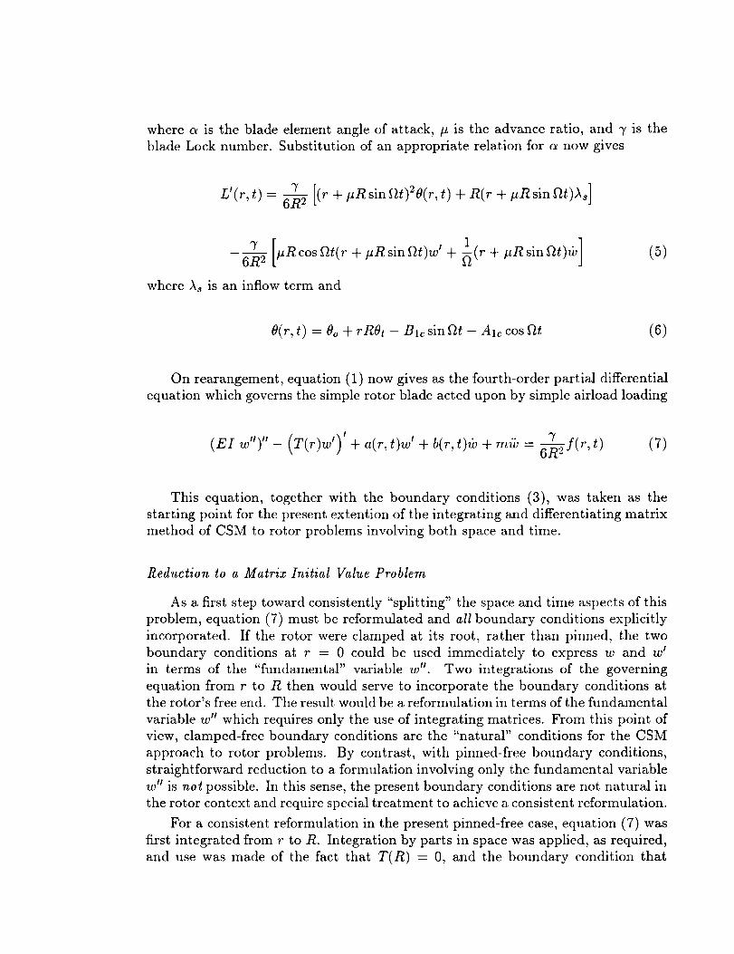
where a is the blade element angle of attack, # is the advance ratio, and 7 is the

blade Lock number. Substitution of an appropriate relation for _ now gives

L'(r,t)- 3' [(r + #Rsinf_t)28(r,t)+ R(r + #R sin f/t)A_]6R 2

3" f

[#R cos f_t(r +6R 2

where As is an inflow term and

1

#Rsinf_t)w _ + -_(r + #n sin gtt)tb] (5)

8(r, t) = 8o + rRSt - Blc sin f_t -Alc cos ftt (6)

On rearangement, equation (1) now gives as the fourth-order partial differential

equation which governs the simple rotor blade acted upon by simple airload loading

3'(EIw')'-(T(r)w')'+a(r,t)w' +b(r,t)(v+rn_= -_sf(r,t) (7)

This equation, together with the boundary conditions (3), was taken as the

starting point for the present extention of the integrating and differentiating matrix

method of CSM to rotor problems involving both space and time.

Reduction to a Matrix Initial Value Problem

As a first step toward consistently "splitting" the space and time aspects of this

problem, equation (7) must be reformulated and all boundary conditions explicitly

incorporated. If the rotor were clamped at its root, rather than pinned, the two

boundary conditions at r = 0 could be used immediately to express w and w I

in terms of the "fundamental" variable w'. Two integrations of the governing

equation from r to R then would serve to incorporate the boundary conditions at

the rotor's free end. The result would be a reformulation in terms of the fundamental

variable w" which requires only the use of integrating matrices. From this point of

view, clamped-free boundary conditions are the "natural" conditions for the CSM

approach to rotor problems. By contrast, with pinned-free boundary conditions,

straightforward reduction to a formulation involving only the fundamental variable

w" is not possible. In this sense, the present boundary conditions are not natural in

the rotor context and require special treatment to achieve a consistent reformulation.

For a consistent reformulation in the present pinned-free case, equation (7) was

first integrated from r to R. Integration by parts in space was applied, as required,

and use was made of the fact that T(R) = 0, and the boundary condition that

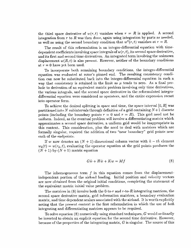
the third space derivative of w(r,t) vanishes when r = R is applied. A second

integration from r to R was then done, again using integration by parts as needed,

as well as using the second boundary condition that w'(r, t) vanishes at r = R.

The result of this reformulation is an integro-differential equation with time-

dependent coefficients involving space integrals of w(r, t), its second space derivative,

and its first and second time derivatives. An integrated term involving the unknown

displacement w(R, t) is also present. However, neither of the boundary conditions

at r = 0 have yet been used.

To incorporate both remaining boundary conditions, the integro-differential

equation was evaluated at rotor's pinned end. The resulting consistency condi-

tion can now be substituted back into the integro-differential equation in such a

way that consistency is retained in the limit as # tends to zero. As a final pre-

lude to derivation of an equivalent matrix problem involving only time derivatives,

the various integrals, and the second space derivative in the reformulated integro-

differential equation were considered as operators, and the entire expression recast

into operator form.

To achieve the desired splitting in space and time, the space interval [0, R] was

partitioned into N subintervals through definition of a grid containing N + 1 discrete

points (including the boundary points r = 0 and r = R). This grid need not be

uniform. Indeed, as the eventual problem will involve a differentiating matrix which

approximates a second space derivative, a uniform grid would be inappropriate in

this context. This consideration, plus the need to deal with matrices which are

formally singular, required the addition of two "near boundary" grid points near

each of the endpoints.

If w now denotes an (N + 1)-dimensional column vector with k - th element

wk(t) = w(rk, t), evaluating the operator equation at the grid points produces the

(N + 1)-by-(N + 1) matrix equation

Gib + H(v + Kw = M f (s)

The inhomogeneous term f in this equation comes from the displacement-

independent portion of the airload loading. Initial position and velocity vectors

are now obtained from the original initial conditions, completing the statement of

the equivalent matrix initial value problem.

The matrices in (8) involve both the 0-to-r and r-to-R integrating matrices, the

second space derivative matrix, grid information matrices, a boundary evaluation

matrix, and time dependent scalars associated with the airload. It is worth explicitly

noting that the present context is the first reformulation in which the use of both

integrating and differentiating matrices appears to be required.

To solve equation (8) numerically using standard techniques, G would ordinarily

be inverted to obtain an explicit equation for the second time derivative. However,

because of the properties of the integrating matrix, G is singular. The source of this

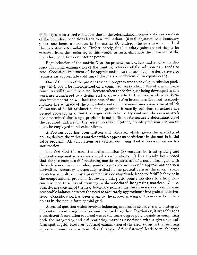
difficulty canbe traced to the fact that in the reformulation, consistentincorporationof the boundary conditions leadsto a "redundant" (0 = 0) equation at a boundary

point, and hence a zero row in the matrix G. Indeed, this is almost a mark of

the consistent reformulation. Unfortunately, this boundary point cannot simply be

removed from the vector w, as this would, in turn, eliminate the influence of the

boundary conditions on interior points.

Regularization of the matrix G in the present context is a matter of some del-

icacy involving examination of the limiting behavior of the solution as r tends to

zero. Consistent treatment of the approximation to the second space derivative also

requires an appropriate splitting of the matrix coefficient K in equation (8).

One of the aims of the present research program was to develop a solution pack-

age which could be implemented on a computer workstation. Use of a mainframe

computer will thus not be a requirement when the techniques being developed in this

work are transferred to a design and analysis context. However, while a worksta-

tion implementation will facilitate ease of use, it also introduces the need to closely

monitor the accuracy of the computed solution. In a mainframe environment which

allows use of 64-bit arithmetic, single precision is usually sufficient to achieve the

desired accuracy in all but the largest calculations. By contrast, the current work

has determined that single precision is not sufficient for accurate determination of

the required matrices in the present context. Rather, double precision arithmetic

must be employed in all calculations.

A Fortran code has been written and validated which, given the spatial grid

points, derives the various matrices which appear as coefficients in the matrix initial

value problem. All calculations are carried out using double precision on an Irisworkstation.

The fact that the consistent reformulation (8) contains both integrating and

differentiating matrices raises special considerations. It has already been noted

that the presence of a differentiating matrix requires use of a nonuniform grid with

the inclusion of near boundary points to preserve accuracy in approximations to a

derivative. Accuracy is especially critical in the present case as the second space

derivative is multiplied by a parameter whose magnitude leads to "stiff" behavior in

the computational problem. However, placing grid points too close to a boundary

can also lead to a loss of accuracy in the associated integrating matrices. Conse-

quently, the spacing of the near boundary points must be chosen so as to achieve an

acceptable balance between the need to accurately approximate integrals and deriva-

tives. Consideration has been given to the proper spacing of these near boundary

points in the nonuniform spatial grid.

A second question which involves balancing accuracies also arises when integrat-

ing and differentiating matrices must be used together. Previously, it was felt that

a consistent formulation required use of the same degree polynomials in computing

both the integrating and differentiating matrices associated with a given nonuni-

form spatial grid. However, a formal examination of the error terms in the resulting

approximations has now shown that this type of "consistency" leads to much larger

errors in approximations to derivatives than to integrals. The larger errors are fur-ther exacerbatedin the present context by the large magnitude of the coefficientwhich multiplies the secondspacederivative matrix. Achieving consistency in theerrors associatedwith an integration and a differentiation has now been shown toimply that polynomials of degreek + 2 must be used to form a differenting matrix

if polynomials of degree k are used to form the corresponding integrating matrix.

Lagrange interpolation was also found to be a more robust method for obtaining

the rows of the first and second space derivative matrices. The previous technique,

involving least squares approximation based on polynomials which are orthogonal

on the discrete grid, remains the preferred technique for the creation of integrating

matrices.

While accuracy considerations are present in the calculation of the basic inte-

grating and differentiating matrices for grids with near-boundary points, features

of the equivalent time-dependent initial value problem also require great care if the

computed solution is not to be contaminated by a large accumulation of numerical

errors. As has been noted, because the ratio of parameters E__Zis large, the ini-m

tial value problem is numerically "stiff." In mathematical terms, this means that

the Jacobian matrix of the system of differential equations has eigenvalues whose

magnitudes differ greatly in size. Physically, solutions of the equations will contain

components which show significant changes on highly disparate time scales. To re-

tain accuracy using standard numerical techniques, the time step used must be that

associated with the fastest time scale. A calculation based on, say, Runge-Kutta

methods, will thus be both highly laborious and inefficient, requiring perhaps thou-

sands of time steps per rotor revolution. Stiff systems require special techniques

for their numerical solution. To solve the present initial value system, a version of

Gear's method for stiff differential equations was implemented on an Iris workstaion.

Spurious oscillations present in earlier solution attempts have now been traced

to the effect of stiffness on slightly imbalanced initial conditions. In particular,

in earlier solutions, the rotor was initially taken as having a polynomial function

as an initial displacement, but no initial velocity. The attempt of transients in the

solution to rapidly modify the initial conditions to give consistent dispacements and

velocities is now thought to have produced large accelerations, which prior numerical

methodology was unable to reconcile. To avoid this hazard of the stiff system, fully

consistent initial conditions on both displacement and velocity (associated with

a normal mode of the unforced, nonrotating pinned-free beam) were used in testcalculations.

Developments During The Funded Period

Lagrange Approach to Differentiating Matricea

The previous computation of the differentiating matrices which approximate

first and second space derivatives at points of the nonuniform grid used least squares

polynomials constructed from a basis set of polynomials which are orthognal with

respectto summations on the discrete grid. As previously formulated, the maximum

degree of the approximating polynomials was seven. Thus, eight grid points atmost could be used to obtain non-zero elements in each row of the matrices. For

the present purposes, this upper limit was found to be inadequate. To achieve the

desired accuracy, seventh degree polynomials must be used in the construction of

integrating matrices. However, to calculate the corresponding second derivative

matrix with a consistent error estimate, tenth degree polynomials must be used.

The present differentiating matrix routine was thus extended to higher degree.

Lagrange interpolation was found to be a highly robust method for accom-

plishing this extension. Whereas general Lagrange coefficients are quite difficult

to integrate (and thus impractical for use in deriving integrating matrices), their

derivatives evaluated at grid points have relatively simple expressions. Further, La-

grange interpolation gives rise to explicit error estimates for approximations to both

first and second derivatives at grid points. However, it was also determined that

use of the higher degree interpolating polynomials may require a re-examination of

the appropriate positioning of near-boundary points in the grid.

Treatment of the Pinned Boundary and Regularization

When the reformulated integro-differential equation for the forced rotating beam

is discretized at the grid points to produce the matrix initial value problem, the

equation associated with the pinned end of the beam vanishes identically because

of consistent incorporation of the boundary conditions. This leaves a system with

more unknowns than equations. In previous work, to achieve a system with as

many equations as unknowns (and hence unique solutions and a regularized matrix

G), a boundary condition at the pinned end was explicitly invoked to delete the

first column of the various coefficient matrices. This resulted in a modified N-by-

N matrix system. However, it was realized in the course of this work that, while

consistent in the setting of a continuous space variable, in the discretized setting

on the spatial grid, this procedure impairs the ability of the matrices involved to

accurately approximate the corresponding integral and differential operators in the

continuous equations. The differentiating matrix is particularly affected by this

deletion, as the positive effect on accuracy of including near-boundary points is

largely negated.

Two implict ways of treating the pinned boundary, which do not involve deletion

of columns in coefficient matrices, were explored. Both approaches regularize the

problem by appending a non-redundant equation to give a modified and invertible

matrix G. In the first approach, an equation setting the second time derivative of

the boundary displacement to zero is appended to the system as the (N + 1)-st

equation. Zero initial displacement and velocity conditions are also imposed at the

pinned end. This has the effect of explicitly imposing the boundary condition spec-

ifying zero displacement at the pinned end. In the second approach, a consistency

condition for the displacement at the free end, which emerges during the reformula-

tion of the original partial differential equation, is appended as the equation which

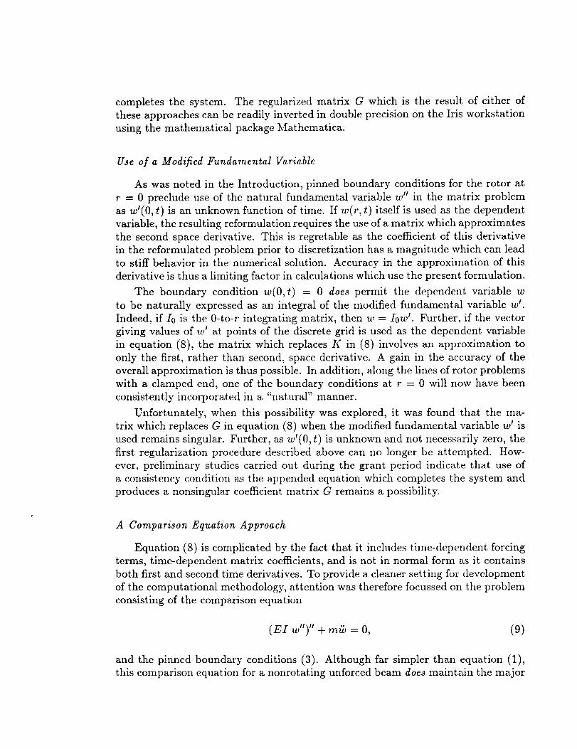
completes the system. The regularized matrix G which is the result of either of

these approaches can be readily inverted in double precision on the Iris workstation

using the mathematical package Mathematica.

Use of a Modified Fundamental Variable

As was noted in the Introduction, pinned boundary conditions for the rotor at

r = 0 preclude use of the natural fundamental variable w" in the matrix problem

as w'(0, t) is an unknown function of time. If w(r, t) itself is used as the dependent

variable, the resulting reformulation requires the use of a matrix which approximates

the second space derivative. This is regretable as the coefficient of this derivative

in the reformulated problem prior to discretization has a magnitude which can lead

to stiff behavior in the numerical solution. Accuracy in the approximation of this

derivative is thus a limiting factor in calculations which use the present formulation.

The boundary condition w(O,t) = 0 does permit the dependent variable w

to be naturally expressed as an integral of the modified fundamental variable w _.

Indeed, if I0 is the 0-to-r integrating matrix, then w = Iow _. Further, if the vector

giving values of w _ at points of the discrete grid is used as the dependent variable

in equation (8), the matrix which replaces K in (8) involves an approximation to

only the first, rather than second, space derivative. A gain in the accuracy of the

overall approximation is thus possible. In addition, along the lines of rotor problems

with a clamped end, one of the boundary conditions at r = 0 will now have been

consistently incorporated in a "natural" manner.

Unfortunately, when this possibility was explored, it was found that the ma-

trix which replaces G in equation (8) when the modified fundamental variable w I is

used remains singular. Further, as wt(0, t) is unknown and not necessarily zero, the

first regularization procedure described above can no longer be attempted. How-

ever, preliminary studies carried out during the grant period indicate that use of

a consistency condition as the appended equation which completes the system and

produces a nonsingular coefficient matrix G remains a possibility.

A Comparison Equation Approach

Equation (8) is complicated by the fact that it includes time-dependent forcing

terms, time-dependent matrix coefficients, and is not in normal form as it contains

both first and second time derivatives. To provide a cleaner setting for development

of the computational methodology, attention was therefore focussed on the problem

consisting of the comparison equation

(EI w')" + m_ = O, (9)

and the pinned boundary conditions (3). Although far simpler than equation (1),

this comparison equation for a nonrotating unforced beam does maintain the major

features of the larger problem, including the inability to use w" as a fundamental

variable and the need to use both integrating and differentiating matrices in the

equivalent matrix initial value problem. Further, the pinned-free beam problem

involving (9) has the distinct advantage that it can be solved exactly. In particular,solutions are of the form

w(r,t) = A(sin )_x + Bsinh_x)(sinwt + C cos_ot), (10)

,_2 with u 2 -- EI and A is a root ofwhere A, B, and C are arbitrary constants, co = -b-- - -N-

the transcendental equation

tan AR - tanh A/_ = 0, (11)

The first few positive solutions of (11) are

= 0.14023580, 0.25244942, 0.36464909

Additional positive values for A are accurately represented by the asymptotic result

7r

An = 4----_(4n + 1), (12)

Thus, using (9) through (12) and appropriate initial conditions, numerical solu-

tions for the comparison problem can be computed, verified, and the associated

computational procedure validated.

The reformulated matrix initial value problem corresponding to (9) and (3) isof the form

where G is the _ame matrix as in equation (8) and D2 is the differentiating matrix

which approximates second derivatives. Work was begun implementing a solution

of the initial value problem composed of (13) and consistent initial conditions using

Gear's method for stiff systems of equations. It was intended that results from

the two approaches to regularizing the matrix G would be compared for feasability,

efficiency and accuracy, and that Mathematica would be used to obtain the inverse

matrix G -1. When equation (13) is left-multiplied by G -1 to obtain an explicit

system for the vector/b,

(v = (ff_-) G-lD2w, (14)

it appearsthat the first andlast rowsand columnsof G -1 must be zeroed to enforce

the boundary conditions w"(0, t) = w"(R, t) = O.

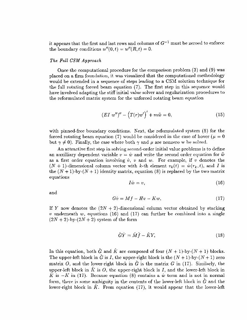
The Full CSM Approach

Once the computational procedure for the comparison problem (3) and (9) was

placed on a firm foundation, it was visualized that the computational methodology

would be extended in a sequence of steps leading to a CSM solution technique for

the full rotating forced beam equation (7). The first step in this sequence would

have involved adapting the stiff initial value solver and regularization procedures to

the reformulated matrix system for the unforced rotating beam equation

(EI w")"- (T(r)w')' + rn/b = 0, (15)

with pinned-free boundary conditions. Next, the reformulated system (8) for the

forced rotating beam equation (7) would be considered in the case of hover (# = 0

but 7 _ 0). Finally, the case where both 7 and # are nonzero w be solved.

An attractive first step in solving second-order initial value problems is to define

an auxilliary dependent variable v = w and write the second order equation for/b

as a first order equation involving /_, v and w. For example, if v denotes the

(N + 1)-dimensional column vector with k-th element vk(t) = (v(rk,t), and I is

the (N + 1)-by-(N + 1) identity matrix, equation (8) is replaced by the two matrix

equations

±_=v, (16)

and

GiJ = M f - Hv - Kw, (17)

If Y now denotes the (2N + 2)-dimensional column vector obtained by stacking

v underneath w, equations (16) and (17) can further be combined into a single

(2N + 2)-by-(2N + 2) system of the form

of = z0?- a-Y, (18)

In this equation, both G and/_ are composed of four (N + 1)-by-(N + 1) blocks.

The upper-left block in (_ is I, the upper-right block is the (N + 1)-by-(N + 1) zero

matrix O, and the lower-right block in (_ is the matrix G in (17). Similarly, the

upper-left block in it" is O, the upper-right block is I, and the lower-left block in

K is -K in (17). Because equation (8) contains a tb term and is not in normal

form, there is some ambiguity in the contents of the lower-left block in G and the

lower-right block in K. From equation (17), it would appear that the lower-left

block in G is O while the lower-right block in /_" is -H. Indeed, this is a valid

possibility. However, (17) can also be written in the form

Hd, + Gb = M f - Kw, (19)

in which case the contents of these two blocks are reversed to H and O. Additional

possibilities include splitting the matrix H in (17) into a sum H = -H1 + H2, in

which case the lower-left block of G in (18) will contain H1 and the lower-right

block of/_2 will be//2.

In solving the reformulated system corresponding to (8) with 7 and # both

nonzero, it is be necessary to explore the possibilities detailed above for the two

blocks in d/ and/_ in order to gauge the effect of each choice on the accuracy of

the evolving solution. On the basis of preliminary work completed during the grant

period, a choice which seems to hold particular promise is to split the matrix H so

that H1 contains the portions of this coefficient which are independent of time.

Final Remarks

Work completed to date on this project indicates that a CSM approach to

rotating beam dynamics using integrating and differentiating matrices holds the

promise of providing a robust solution methodology which would be of great value

in an engineering design environment. Unfortunately, because of reorganization of

units at Langley Research Center, the group which has supported this promising

reseach in the past has now disappeared. While an attempt will be made to continue

development of the present CSM approach, its eventual evolution into an engineering

design tool can no longer be assured.

References

[1] M.B. Vakhitov, Integrating matrices as a means of numerical solution of differ-

ential equations in structural mechanics. Isvestiya VUZ. Aviatsionnaya Teknika

3, 50-61 (1966).

[2] W.F. Hunter, The integrating matrix method for determining the natural vi-

bration characteristics of propeller blades. NASA TN D-6064, December, 1970.

[3] R.G. Kvaternik, W.F. White, Jr. and K.R.V. Kaza, Nonlinear flap-lag-axial

equations of a rotating beam with arbitrary precone angle. Presented at the

AIAA/ASME 19th Structures, Structural Dynamics, and Materials Conference,

Bethesda, Maryland (AIAA Paper 78-491), April, 1978.

[4] W.F. White, Jr., R.G. Kvaternik and K.V. Kaza, Buckling of rotating beams.

International Journal of Mechanical Sciences 21,739-745 (1979).

[5] W.D. Lakin, Integrating matrices for arbitrarily spaced grid points. NASA

CR-159172, November, 1979.

[6] W.D. Lakin, Differentiating matrices for arbitrarily spacedgrid points. Inter-

national Journal for Numerical Methods in Engineering 23, 209-218 (1986).

[7] W.D. Lakin, A differentiating and integrating matrix approach for the bihar-

monic eigenvalue problems of vibrating elastic plates. Journal of Engineering

Mathematics 20, 203-215 (1986).

[8] W.D. Lakin and R.G. Kvaternik, An integrating matrix formulation for buckling

of rotating beams including tile effects of concentrated masses. International

Journal of Mechanical Sciences 31,569-577 (1989).

[9] F.D. Harris, Derivation of the equation for flap bending, Appendix to memo

dated August 24, 1987.