
C/SiC HX Thermal and Mechanical Analysis · 2018-02-13 · Pro/Mechanica module (Pro/M) in the...
36
Pg. 1 of 36 C/SiC HX Thermal and Mechanical Analysis Wensheng Huang, Per F. Peterson, and Haihua Zhao U.C. Berkeley Report UCBTH-05-004 September 30, 2005 2nd Deliverable Report for Year 04-to-05, DOE NHI HTHX Project ABSTRACT This report summarizes UCB’s initial results and methods on C/SiC heat exchanger thermal and mechanical analysis for high temperature heat transfer under support from DOE National Hydrogen Initiative program (NHI) through UNLV HTHX project, as a part of efforts for nuclear hydrogen production. The intermediate heat exchanger (IHX) transfers heat from high temperature high pressure helium to a liquid salt intermediate loop which couples to hydrogen production loops. The IHXs operates at temperature from 600°C to 1000°C and pressure difference up to 8 MPa. The operating conditions are extremely challenging for metals to function in, while it is not challenging for carbon and silicon carbide composites. To be economically viable for hydrogen production, ceramic heat exchangers must have costs under a few tens of dollars per thermal kilowatt. Plate-type ceramic heat exchanger with relatively small flow channels provide a good candidate approach for this purpose, because they can obtain high power densities and low mechanical stresses with thin heat transfer surfaces and small amounts of material. Thermal and stress analysis are carried out to identify optimal designs for core heat transfer unit, inlet and outlet manifolds, distribution channels, and channel dividers. Finding detailed stress distribution in a complete heat exchanger with direct FEM (Finite Element Method) requires an order of billion FEM computation units and million hours PC computing time. Therefore, it is not practical to analyze the entire heat exchanger design directly. We propose an alternative method to obtain approximate stresses that only requires several days to finish in a fast PC. The methods are composed of three steps. First, the heat exchanger is broken down into several regions. Unit cell models are built based on each region that captures all of the most important features of that region. The effective mechanical and thermal properties for each unit cell are then founded through FEM simulations. Second, average stress distribution in an overall model composed of various unit cell regions is computed by using the effective mechanical and thermal properties. Third, these average stress values are then applied to the unit cells to find localized points of high stresses. Pro/Mechanica module (Pro/M) in the Pro/E Wildfire Edition is used for FEM stress analysis.
Transcript of C/SiC HX Thermal and Mechanical Analysis · 2018-02-13 · Pro/Mechanica module (Pro/M) in the...

Pg. 1 of 36
C/SiC HX Thermal and Mechanical Analysis
Wensheng Huang, Per F. Peterson, and Haihua Zhao
U.C. Berkeley
Report UCBTH-05-004
September 30, 2005
2nd Deliverable Report for Year 04-to-05, DOE NHI HTHX Project
ABSTRACT
This report summarizes UCB’s initial results and methods on C/SiC heat
exchanger thermal and mechanical analysis for high temperature heat transfer under
support from DOE National Hydrogen Initiative program (NHI) through UNLV HTHX
project, as a part of efforts for nuclear hydrogen production. The intermediate heat
exchanger (IHX) transfers heat from high temperature high pressure helium to a liquid
salt intermediate loop which couples to hydrogen production loops. The IHXs operates at
temperature from 600°C to 1000°C and pressure difference up to 8 MPa. The operating
conditions are extremely challenging for metals to function in, while it is not challenging
for carbon and silicon carbide composites. To be economically viable for hydrogen
production, ceramic heat exchangers must have costs under a few tens of dollars per
thermal kilowatt. Plate-type ceramic heat exchanger with relatively small flow channels
provide a good candidate approach for this purpose, because they can obtain high power
densities and low mechanical stresses with thin heat transfer surfaces and small amounts
of material. Thermal and stress analysis are carried out to identify optimal designs for
core heat transfer unit, inlet and outlet manifolds, distribution channels, and channel
dividers. Finding detailed stress distribution in a complete heat exchanger with direct
FEM (Finite Element Method) requires an order of billion FEM computation units and
million hours PC computing time. Therefore, it is not practical to analyze the entire heat
exchanger design directly. We propose an alternative method to obtain approximate
stresses that only requires several days to finish in a fast PC. The methods are composed
of three steps. First, the heat exchanger is broken down into several regions. Unit cell
models are built based on each region that captures all of the most important features of
that region. The effective mechanical and thermal properties for each unit cell are then
founded through FEM simulations. Second, average stress distribution in an overall
model composed of various unit cell regions is computed by using the effective
mechanical and thermal properties. Third, these average stress values are then applied to
the unit cells to find localized points of high stresses. Pro/Mechanica module (Pro/M) in
the Pro/E Wildfire Edition is used for FEM stress analysis.

Pg. 2 of 36
1. INTRODUCTION
Nuclear hydrogen production requires an IHX to transfer high temperature heat from high
temperature gas cooled reactor to an intermediate loop which couples with hydrogen
production loops. The IHXs operates at temperature from 600°C to 1000°C and pressure
difference up to 8 MPa. The operating conditions are extremely challenging for metals to
function in, while it is not challenging for carbon and silicon carbide composites. LSI and
PI carbon-carbon composites can maintain nearly full mechanical strength at high
temperatures (up to 1400°C), have low residual porosity and are compatible with molten
salt and high-pressure helium [1]. These materials are relatively simple to fabricate and
have relatively low cost. To be economically viable for hydrogen production, ceramic
heat exchangers must have costs under a few tens of dollars per thermal kilowatt. Plate-
type ceramic heat exchanger with relatively small flow channels provide a good
candidate approach for this purpose, because they can obtain high power densities and
low mechanical stresses with thin heat transfer surfaces and small amounts of material.
To fabricate compact plate-type heat exchangers, one side of each plate is die-
embossed or milled, to provide appropriate flow channels, leaving behind fins or ribs that
would provide enhanced heat transfer, as well as the mechanical connection to the
smooth side of the next plate. For green carbon-carbon material, milling can be
performed readily with standard numerically controlled milling machines. Alternatively,
plates can be molded with flow channels, as has been demonstrated for carbon-carbon
composite plates fabricated at ORNL for fuel cells [2]. For assembly, the ends of the fins
and other remaining unmachined surfaces around the machined flow channels would be
coated with phenolic adhesive, the plate stack assembled, header pipes bonded and
reinforced, and the resulting monolith pyrolysed under compression. Then liquid silicon
or polymers would be infiltrated to reaction bond the plates and headers together, forming
a compact heat exchanger monolith.
Figure 1 illustrates discontinuous fin geometry for molten salt-to-helium compact
heat exchangers. The cross-sectional area of the fins and the thickness of the remaining
plate below the machined channels would be adjusted to provide sufficient strength to
resist thermal and mechanical stresses. For the case in which the heat exchanger is
immersed into a helium environment, detailed unit cell stress analysis as shown in Figure
2 has indicated that the stresses are dominantly compressive and can be accommodated
with relative ease. Figure 3 shows a preliminary draft plate design for the compact offset
fin plate heat exchangers. Helium plates and molten salt plates are alternatively joined
together to form a heat exchanger module. This design is applicable to compact
counterflow heat exchanger, where there is a substantial difference between the
volumetric flow rates of the two fluids. Applications can include liquid-to-gas heat
exchangers and gas-to-gas heat exchangers where there exists a large difference in the
volumetric flow rates. The helium side plate has several equal spacing flow dividers to
reduce flow maldistribution. Earlier preliminary mechanical stress analysis shows that the
stress on the helium divider in the distribution region is very low. Most of it comes from
the compressive force of high pressure helium on the divider itself. Global mechanical
stress analysis and thermal stress analysis are carried out in this study.

Pg. 3 of 36
Figure 1: Cut away view through a plate showing alternating molten salt (top and bottom arrows) and
helium (middle arrows) flow channels. Dark bands at the top of each fin indicate the location of reaction-
bonded joints between each plate.
Figure 2: Stress and temperature distributions in a plate type LSI composite heat exchanger.
Reaction-bondedjoint
CVI/CVDcarbon-coatedMS surfaceMilled or
die-embossedflow channel
Milled or die embossed He flow channel
Reaction-bonded joint
Low-permeability coating(optional)
Milled or die embossed MS flow channel
SIDE VIEW
PLAN VIEW
Px
l
w
Py
Radius at corner
Radius at corner
hHedHe
hMSdMS Reaction-bondedjoint
CVI/CVDcarbon-coatedMS surfaceMilled or
die-embossedflow channel
Reaction-bondedjoint
CVI/CVDcarbon-coatedMS surfaceMilled or
die-embossedflow channel
Milled or die embossed He flow channel
Reaction-bonded joint
Low-permeability coating(optional)
Milled or die embossed MS flow channel
SIDE VIEW
PLAN VIEW
Px
l
w
Py
Radius at corner
Radius at corner
hHedHe
hMSdMS

Pg. 4 of 36
Figure 3: Plates design for compact offset fin plate heat exchanger.
CAD design and analysis software Pro/Engineer (Pro/E) is used for 3-D design,
thermal and mechanical analyses of the offset fin compact plate heat exchangers. Pro/E
has the advantage of combining design and analysis work together. Pro/Mechanica
module (Pro/M) in the Pro/E Wildfire Edition is used for stress analysis. Pro/M uses p-
type finite elements (FEM) to compute its solution [3]. One of the key advantages of p-
type finite elements is that they allow solution adaptivity without requiring mesh
refinement. With standard “h-type” finite elements, once a solution is obtained, the only
way to improve its quality consists of repeating the calculation using a finer mesh - this
process is well known to be time consuming, complex and problematic in several ways.
In contrast, with p-type elements, the maximum polynomial orders of basis functions
used to approximate the solution can be increased locally as needed. The solution process
can then be repeated on the same mesh, with the new increased polynomial orders. Such
an adaptivity step (often called a pass in Pro/M) can be repeated, if desired, to achieve
even greater accuracy. In the p-type finite element method, basis functions are
constructed in a way that the maximum polynomial order of approximation can be
selected independently for each edge, face, and solid in the mesh. Pro/M selects
polynomial orders independently for each edge, and the polynomial order of
approximation on each face and solid is then selected based on the choices made for the
underlying edges. Therefore, the goal of a p-order adaptivity method consists of selecting
appropriate polynomial orders for each edge that will lead to an overall solution
providing good quality results using acceptable elapsed time and computing resource.
molten salt side plate helium side plate
helium inlet
Molten salt inlet
Molten salt outlet
molten salt side plate helium side plate
helium inlet
Molten salt inlet
Molten salt outlet

Pg. 5 of 36
Although finite element analysis is capable of finding accurate results over
various kinds of geometries, for complex geometries the amount of time needed to
process finite-element models can become prohibitively large. As the number of
polygons and the order of equations fitted increase, the number of equations that must be
solved increases exponentially. For example, finding the stresses accurate to 10% on a
600-polygon unit cell model can take up to 30 minutes on the fastest personal computer.
One unit cell in the core heat transfer region has length scale about 1 cm. The total length
scale for a compact heat exchanger is 1 m. Entire heat exchanger needs 6 · 108 polygons.
Finding detailed stress distribution in a complete heat exchanger with direct FEM (Finite
Element Method) requires an order of million hours PC computing time. Therefore, it is
not practical to analyze the entire heat exchanger design directly. We propose an
alternative approach that gives slightly less accurate results but is more versatile and far
less time consuming. The following part describes the basic ideas.
The compact plate fin heat exchanger is composed of many alternating Molten
Salt (MS) and Helium (He) plates. For stress analysis, each pair of heat exchanger plates
is basically identical. So only one pair of plates (one MS plate and one He plate) is
needed for the purpose of stress analysis. To analyze the steady-state thermal and
mechanical stresses in a full-size high temperature heat exchanger module, one pair of
plates in the heat exchanger is broken down into multiple similar regions. Unit cell
models are built based on each region that captures all of the most important features of
that region. Figure 4 shows the various regions that are grouped together because of
similar features. Figure 5 shows pictures of the unit cell models built from the regions
defined in figure 4. In order from left to right, top to bottom, they are unit cells A, B, C,
and D. These models are called unit cells because when one reflects each cell across its
six boundary surfaces one can recreate the geometry found in the corresponding region.
In other words, the unit cells all have cubic symmetry. Note that one can only create unit
cells out of regions that have symmetrical patterns. Certain approximations need to be
applied when a region cannot be recreated from symmetrical unit cells. For example, unit
cell A has round fillets on the inner edge in its top portion but no rounds in the bottom.
Yet this cell will give approximately the right answer because the rounds represent a
relatively small mass compared to the main body of the cell. This and other
approximations employed are pointed out in appropriate locations of this report.

Pg. 6 of 36
Figure 4: Division of unit cell model regions in a plate.
Figure 5: Unit cell models.

Pg. 7 of 36
The methods we use to obtain approximate thermal and mechanical stresses are
composed of three steps. First, the effective mechanical and thermal properties for each
unit cell are founded through various FEM simulations; Second, average stress
distribution in an overall model composed of various unit cell regions is computed by
using the effective mechanical and thermal properties; Third, these average stress values
are then applied to the unit cells to find localized points of high stresses. For example, if
the result of average stress analysis shows that region A has a maximum compressive
stress of -15 MPa (all compressive stresses are written as negative numbers), an overall
pressure of 15 MPa is applied across all six surfaces of unit cell A. The maximum
compressive stress found in the unit cell A in this FEM simulation would be the max
actual local compressive stress in region A. This also pinpoints locations where stresses
are greatest. Similar method is employed to find the maximum tensile stress.
2. EFFECTIVE MECHANICAL AND THERMAL PROPERTIES FOR UNIT
CELLS
2.1 Normal Stress Moduli
Assumptions
A unit cell is orthotropic, which means it deforms in different ways along each of its
three axes (3 Young’s moduli, 3 Poisson ratios, 3 Shear moduli). The material that made
up the unit cell is uniform and isotropic. Helium pressure is 10 MPa and MS pressure is
0.1 MPa.
The Models
Four models are used to find all relevant normal stress moduli, one for each unit cell.
The model for unit cell A is used here as an example to show how the unit cell models
are created. Unit cell A is set up to include one salt channel and one helium channel, one
salt fin and one helium fin. The model is created by having a symmetry plane (normal to
z-axis) cuts a fin in half at its waist, and another symmetry plane (normal to x-axis) cuts
the staggered fin along the middle. The third symmetry plane, which is normal to the y-
axis, cuts in the middle of the MS and HE plate. Despite the root of the fins being
rounded and the top being un-rounded, the two sides of the third symmetry plane are
approximately the same. This is one of the unit cell approximations previously mentioned
in the procedure. Unit cells B, C, and D were created on the same principles as A, any
differences and approximations will be noted in Appendix A.
Constraints
The process of assigning constraints is described here using unit cell A as an example.
On each face of the unit cell, a rigid flat plane is imposed. To make sure it was rigid and
flat, translation in the direction of corresponding axis is fixed, while rotations in the other
2 axes are fixed. The other 3 degrees of freedom are freed. The constraint surface
normal to the x-axis on the positive x side is called X1, the constraint surface parallel to

Pg. 8 of 36
X1 but is on the negative x side is called X2. Similarly, the other 4 constraint surfaces
are called Y1, Y2, Z1, and Z2. Initially, the constraint surfaces are set at zero
displacement so an initial test will show the stresses on the unit cell with no
displacement. Since the moduli are found by calculating change in stress versus change
in strain, it is important to know what the stress is at zero displacement. Subsequent
constraint sets vary the displacements to obtain the moduli.
Loads
The loads used in the model are pressure loads representing the fluid pressure present in
each channel. For the MS channels, 0.1 MPa is used, while 10 MPa is used for He
channel surfaces.
Properties of the heat exchanger materials
Table 1 shows material properties of typical SiSiC composite, which is a potential
material for the compact heat exchangers.
Table 1. Properties of SiSiC
Young’s Modulus [GPa] 300
Poisson Ratio, [-] 0.2
Tensile Strength [MPa] ~300
Coefficient of Thermal Expansion (300 - 1000 ºC) [10-6 /K] 4.5
Heat Conductivity [W/m·K] 40
Density [g/cm3] 3.1
Specific Heat Capacity [kJ/kg·K] 1.1
Methods
The whole process is performed using Pro/M software. Three variables are set up to
track the reactions on the symmetry boundaries (which coincide with the constraint
surfaces). The first variable tracks reaction in the x-direction on the X1 constraint
surface, the second variable y-direction reaction, and etc. For each unit cell, four stress
tests were run in Pro/M. The initial test has zero displacement on all constraint surfaces.
The other three tests were run with the strain described in table 2. The actual
displacement set for each test is equal to strain times the length of the unit cell in the
corresponding direction. For example, unit cell A is 5 mm long so for test 1, the x
displacement for the X1 constraint surface is set to -1.5e-3 mm. The negative
displacement indicates simulated compression. The reported reactions are added to
corresponding channel forces on each face and divided by the total area on that face to
obtain the average stress on that constraint surface. Several matrix calculations were
carried out to obtain all nine normal stress moduli.

Pg. 9 of 36
Table 2. Strain value used in the four tests for each unit cell
0-displacement Test 1 Test 2 Test 3
X1 0 3e-4 4e-4 5e-4
Y1 0 4e-4 5e-4 3e-4
Z1 0 5e-4 3e-4 4e-4
Matrix Calculations
Based on the results of the four tests performed on each unit cell, the nine normal stress
moduli (Young’s moduli and poison ratios) can be extracted. The relation between stress
and strain is as follows:
ε = D x σ, (1)
Where ε is the strain tensor, σ the stress tensor. The inverse elastic tensor (D) for
orthotropic material is defined as [Reddy, 1999]:
1/Ex - νxy /Ex - νxz /Ex 0 0 0
- νyx /Ey 1/Ey - νyz /Ey 0 0 0
- νzx /Ez - νzy /Ez 1/Ez 0 0 0
0 0 0 1/Gxy 0 0
0 0 0 0 1/Gyz 0
0 0 0 0 0 1/Gzx
Where E is normal stress Young’s modulus, G shear stress modulus, and ν Poisson’s
ratio. For orthotropic material, the stress-strain relation can be rewritten as six equations.
If we only look at the top three equations (the ones that do not involve shear stress), we
see nine variables and three equations. However, if three tests are performed and each
test generates three independent sets of stress and their corresponding strains, nine
equations with nine variables are formed. Simultaneously solving these nine equations
yield the nine variables (the nine normal stress moduli). The zero-displacement test is
needed because the stress-strain relation only works with changes in stresses and changes
in strains, so a reference point is needed to calculate those changes. Detail derivation for
the equations used in matrix calculations is attached in Appendix B.
Results
The unit cell A is taken as an example to show how to find nine moduli. Table 3 shows
the surface areas of the constraint surfaces and the lengths of the unit cell A in the
corresponding axes.

Pg. 10 of 36
Table 3. Geometry data for unit cell A
Solid Surface
Area (mm2)
MS Channel
Area (mm2)
He Channel
Area (mm2)
Total Area
(mm2)
Length of Cell Along
That Axis (mm)
X1 37.26 6.07 12.17 55.5 3
Y1 14.52 18.78 0 33.3 5
Z1 9.12 1.44 4.44 15 11.1
The equation to calculate average stress on each constraint surface is,
σave = (Rs - PMS*AMS - PHe*AHe)/Atotal (2)
Where P is pressure, A surface area, Rs the reaction at corresponding solid face as
reported by Pro/M. The pressure forces are negative because they were forces of the fluid
in surrounding cells. Table 4 shows the results of the four Pro/M stress tests for the unit
cell A.
Table 4. Stress results of Pro/M tests for the unit cell A
σX1 σY1 σZ1
0-displacement -4.606 -5.903 -4.153
Test 1 -69.476 -50.408 -106.530
Test 2 -79.009 -56.125 -76.750
Test 3 -92.479 -44.882 -93.716
From the results and based on the equations in Appendix B, the nine effective normal
stress moduli were calculated as follows,
Eeff,x = 1.310e11 Pa
Eeff,y = 7.110e10 Pa
Eeff,z = 1.634e11 Pa
Poisson Ratios were as follows,
νxy = 0.113
νxz = 0.199
νyx = 0.213
νyz = 0.192
νzx = 0.157
νzy = 0.078 To fully define an orthotropic cell, only three independent Poisson ratios are
needed. νxy, νxz, and νyz can be calculated from νyx, νzx, and νzy. The Poisson ratios in the yx, zx, and zy directions are the ones asked for by Pro/M when entering material
properties so those are the ones that will be used for this method.
In addition to effective moduli, each unit cell has an effective density that must be
taken into account. This number can be easily calculated as a fraction of the density of
the original material based on the volume occupied by the unit cell. Equation 3 can be
used.
ρeff = ρ · (Vs / Vtotal) (3)

Pg. 11 of 36
Where ρeff is effective density of the unit cell, ρ density of the original material, Vs the
solid volume of the unit cell and Vtotal the total volume of the unit cell.
Table 5 summarizes the results of the normal stress test for all four unit cells.
Table 5. Summary of effective normal stress moduli
Unit Cell Eeff,x [Pa] Eeff,y [Pa] Eeff,z [Pa] νyx νzx νzy ρeff [kg/m3]
A 1.310e11 7.11e10 1.634e11 0.2128 0.1575 0.0785 1810
B 1.683e11 8.30e10 1.758e11 0.1937 0.1882 0.0812 2049
C 1.599e11 5.29e10 1.557e11 0.1848 0.1790 0.0685 1835
D 2.702e11 2.103e11 2.499e11 0.2014 0.2002 0.1670 2792
Summary
The requirement for a transversely isotropic unit cell is that two of its Young’s moduli
and two of its Poisson ratios must be approximately the same; furthermore, the two
Poisson ratios must be in the direction of one of the two equal Young’s moduli and the
direction of the third unequal Young’s moduli. Based on table 5, unit cell A is obviously
orthotropic as all three of its Young’s moduli are different. However, B, C, and D seem
to be transversely isotropic since two of their Young’s moduli and two of their Poisson
ratios are equal. But the wrong pairs of Poisson ratios are equal with respect to the pairs
of Young’s moduli that are equal. So these three unit cells must also be orthotropic.
2.2 Shear Stress Moduli
Assumptions
The unit cell is orthotropic. The material that made up the unit cell is uniform and
isotropic.
Methods
The main difference between the shear stress tests and the normal stress tests is that
lateral strain, instead of axial strain, is imposed on the constraint surfaces. For example,
for the test to find Gxy, a displacement in the y-direction is imposed on the X1 face and
the X2 face is constrained in the y-direction; both surfaces are constrained in the x-
direction. Y1 and Y2 would be left free, and Z1 and Z2 would be constrained in the z-
direction. The rotation constraints are set up to allow each surface to rotate in the
direction of their corresponding axes. And the Y surfaces could additionally rotate in the
z-direction. Figure 6 shows how the shear stress test for Gxy on the unit cell A was done.

Pg. 12 of 36
Figure 6: Shear test illustration for Gxy on the unit cell A.
This setup violates the symmetry constraints. It is unfortunate that it seems to be
no way to keep a flat rigid slanted surface boundary on the Y surfaces in Pro/M. To get
good results, it is necessary to approximate the shear moduli. Instead of performing the
shear test on a single unit cell, the test was performed on a large, almost square-shaped
block composed of many unit cells. Two tests were performed for each of the three shear
moduli. The results from the xy and the yx test would be averaged to find the Gxy moduli.
(In orthotropic materials, Gxy = Gyx, the other four shear moduli are paired up in a similar
fashion) By convention, Pro/M accepts Gxy, Gxz, and Gyz, so those are the notations that
will be used for the three shear moduli. Figure 7 is an example of the model used to find
shear moduli on the unit cell A. The more unit cells used to make up the shear test model
the more closely the results of each pair of shear test would agree. However, increasing
the size of the model significantly increases the calculations time so the models used
were around sizes that took about an hour to analyze per run.
Since the strains were set and the reaction forces were reported by Pro/M, the
shear moduli could be found with Equation 4,
G = τ/γ (4)
where G is the shear moduli, τ the shear stress, and γ the physical strain. The physical
strain is obtained by Equation 5,
γxy = arctan (dispX1_Y / Lx) (5)
where dispX1_Y is the displacement of constraint surface X1 in the y-direction and Lx is
the length of the unit cell in the x-direction. For further reference, engineering shear
strain (εxy) is equal to half of physical strain.

Pg. 13 of 36
Figure 7: Shear test model for Gxy on the unit cell A.
Results
Table 6 summarizes the results of the shear stress tests.
Table 6. Summary of effective shear moduli
Unit cell Gxy [Pa] Gxz [Pa] Gyz [Pa]
A 1.89e10 5.99e10 4.18e10
B 3.03e10 6.61e10 2.34e10
C 1.85e10 6.81e10 2.87e10
D 6.69e10 7.35e10 5.02e10
2.3 Thermal Properties
Introduction
Once the mechanical properties of each of the four unit cells are determined, the thermal
properties of those cells must be evaluated. The three important thermal properties for
Pg. 14 of 36
thermal stress analysis are thermal expansion coefficient α, specific heat capacity cp, and
effective thermal conductivity k.
Methods
For orthotropic unit cells, there can be up to three expansion coefficients, one specific
heat capacity, and three conduction coefficients. However, our unit cells are not real
orthotropic materials; they are effectively orthotropic. No matter what shape the unit
cells take on, they would expand the same relative amount in all directions with
temperature changes much like an isotropic cell. The three expansion coefficients are
equal to the expansion coefficient of the original material regardless of unit cell
geometry. An easy way to visualize this is to imagine a cubic unit cell filled with an
isotropic solid material and another cubic unit cell that is made from bars of the same
material lining all twelve edges. Simple math or common sense can tell that under the
same temperature change, the solid cube will expand just as much as the hollow cube
frame will. Geometries of the cube and the frame will not influence the effective
expansion coefficient of each unit cell.
Since specific heat capacity is a measure of how much energy is stored per mass
per temperature change, unit cell geometry once again plays no role. This is why there is
only one specific heat capacity for orthotropic unit cells.
On the other hand, there are three conduction coefficients for our unit cells, and
these coefficients do depend on geometry. Due to limitations in the ability of Pro/M to
output thermal flux data, these coefficients have to be estimated. They are estimated by
taking a fraction of the original material’s thermal conductivity based on smallest cross
sectional area. For example, for the unit cell A in the x-direction, most of the heat energy
is conducted along the plates and not the fins. The plates have a cross-sectional area of
22.2 mm2 in the x-direction, and the total cross-sectional area in the x-direction is 55.5
mm2. The estimated thermal conduction coefficient in the x-direction is equal to 40
W/(m·K) (coefficient value of the original material) times (22.2 / 55.5), which is equal to
16 W/(m·K).
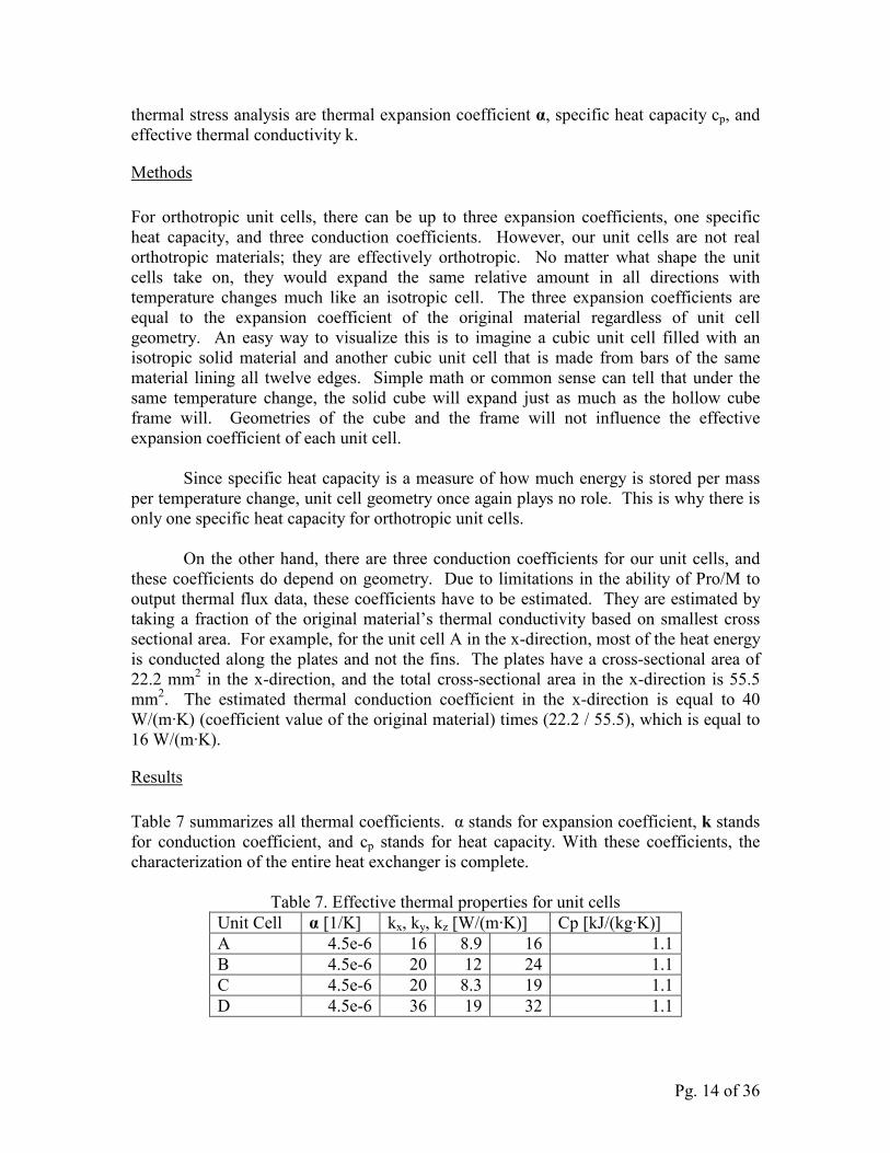
Results
Table 7 summarizes all thermal coefficients. α stands for expansion coefficient, k stands
for conduction coefficient, and cp stands for heat capacity. With these coefficients, the
characterization of the entire heat exchanger is complete.
Table 7. Effective thermal properties for unit cells
Unit Cell α [1/K] kx, ky, kz [W/(m·K)] Cp [kJ/(kg·K)]
A 4.5e-6 16 8.9 16 1.1
B 4.5e-6 20 12 24 1.1
C 4.5e-6 20 8.3 19 1.1
D 4.5e-6 36 19 32 1.1

Pg. 15 of 36
3. OVERALL STEADY-STATE STRESS ANALYSES
Just as a recap, figure 8 shows the overall heat exchanger plate assembly that describes
the original heat exchanger plates. Each region is color coded, and the gray regions
represent the original material (marked as region O). The figure also shows the
constraints that are applied to the overall model. Since the heat exchanger may be free to
expand and contract in real-life, we should use constraints that constrict the free
expansion of the model as little as possible. The Y2 surfaces of the model are restrained
from moving in the y-direction. (Recall that the Y1 face refers to the surface
perpendicular to the y-axis in the positive y-direction, and the Y2 face refers to the
surface in the negative y-direction.) Then either the hot molten salt inlet or the cold
outlet is restrained in the r and θ directions. These constraints mimic what would happen
if either the hot inlet or cold outlet pipe connected to the model are rigid. Results from
these two sets of constraints will be presented separately.
Since the heat exchanger would be submerged in a high pressure helium
environment, the exposed sides of the heat exchanger are assumed to subject to 10 MPa
pressures. The inlet and outlet holes are assumed to subject to pressures of
approximately 1 MPa coming from dense molten salt. The Y2 face had been made
rigidly flat, but to allow for expansion, the Y1 face was given full freedom. To simulate
the pressure from the helium environment in the y-direction we applied a pressure on the
Y1 face that effectively mimicked environmental pressure from helium. By applying a
pressure of 10.62 MPa, the average pressure across the entire Y1 face, counting the
contribution from the inlet/outlet hole, would be equal to 10 MPa.
The thermal load on the overall assembly is based on a simple linear temperature
distribution analysis. That is, the temperature on the MS inlet/outlet and the helium
inlet/outlet are defined and they are assumed to vary linearly across the entire heat
exchanger plate. This assumption is very basic but the results provide some indication of
what kind of stresses the real heat exchanger will experience. Taking a simple thermal
design for AHTR power conversion heater (MS to He heat exchanger) by UCB as an
example, the temperatures on the various inlet and outlet are defined as follows. MS inlet
is set at 925°C, MS outlet is set at 860°C, He inlet is set at 622°C, and He outlet is set at
900°C. The heaters for AHTR power conversion system works in more challenging
environment than a NGNP IHX (higher pressure difference and higher temperature).
Using AHTR heater parameters to study the stresses can give conservative results for
NGNP IHX design.
Pro/M requires that we set a reference temperature in order to properly generate
thermal loading. The reference temperature will be set dependent upon which hole in the
model is being constrained. For the test where the hot inlet is constrained, the reference
temperature will be set at 925 °C, and for the cold outlet test, the reference temperature
will be set at 860 °C. These temperatures were chosen based on the temperature of the
hole being constrained. If one does not pick a reference temperature that is the same as
the hole being constrained, artificial (fake) stresses will be generated as the area around
the constrained hole tries to contract or expand against a fixed hole. In reality, the hole
contracts or expands with the surrounding area.

Pg. 16 of 36
Figure 8: Overall heat exchanger plate model with constraints.
Figure 9 shows the temperature distribution given be Pro/M based on the
previously given temperature constraints. For temperature color scale, white represents
hot and blue represents cold. Figure 10 to 13 show, in order, the maximum principle (XP)
stresses based on constraining the hot MS inlet, the minimum principle (MP) stresses
based on constraining the hot inlet, the XP stresses based on constraining the cold inlet,
and the MP stresses based on constraining the cold inlet. Note that analyses of the
principle stresses were chosen as oppose to Von Mises stresses because the original
material behaves like a ceramic and will fracture if forced to accommodate any
significant tensile strain deformation. The phenomenon of fracturing depends on the
highest compressive (min principle) and tensile (max principle) stresses present in the
material. Also, that the Hot Inlet test refers to the analysis in which the hot MS inlet was
constrained; and the Cold Outlet test refers to the analysis in which the cold MS outlet
was constrained. Also note that the legends are not the same for every graph; the legends
were chosen to highlight important features.

Pg. 17 of 36
Figure 9: Simple linear temperature distribution.
Figure 10: Max principle stress based on Hot Inlet Test.

Pg. 18 of 36
Figure 11: Min principle stress based on Hot Inlet Test.
Figure 12: Max principle stress based on Cold Inlet Test.

Pg. 19 of 36
Figure 13: Min principle stress based on Cold Inlet Test.
Recall that the reason one does analyses on the overall heat exchanger plate
model is to find the maximum average compressive and tensile stresses present in each of
the regions represented by unit cells. However, based on figures 10 to 13, it is apparent
that the majority of unit cell A, B, and C are under an average stress very different from
the maximum and minimum principle stresses. So to get a better picture and how stresses
are distributed in the unit cells, we should take note of the average stresses those regions
are under and do localized stress tests with those average values as well as with the max
and min values. Table 8 summarizes the max, min, and average stresses in each of the
five regions. Max and Min stand for the maximum and the minimum stresses found in
the cell. The Avg (XP, MP) columns contain the average max and min principle stresses
found in the majority of each cell for each test. And the typical stress values are the
average of the averages, representing the typical stress state that the unit cell is in.
Table 8. Summary of stresses in each unit cell (MPa)
Hot Inlet Test Cold Outlet Test Unit Cell
Max Min Avg (XP,MP) Max Min Avg (XP,MP)
Typical Stress
A 0 -14 -9.5, -10.5 0 -15 -9.5, -10.5 -10
B 0 -20 -8, -12 3 -25 -7, -13 -10
C 50 -23 -7, -12 50 -35 -6, -13 -9.5
D 5 -70 N/A 30 -65 N/A N/A
O 75 -130 N/A 130 -30 N/A N/A

Pg. 20 of 36
The reason why we will not do a local stress analysis based on average stress
values on unit cell D is because the stresses on unit cell D varies greatly across the unit
cell, doing an average stress test on unit cell D will not tell us a great deal about the cell.
Unit cell O is just the original material, so there is no need to do local stress analysis on
unit cell O.
It is interesting to see that the average stress values for the hot and cold tests are
nearly identical for unit cell A, B, and C. This suggests that constraining the overall
model by the inlet or by the outlet does not significantly affect the average stresses found
in the central regions. We would expect this from Saint-Venant’s Principle since the
central region is far away from either the inlet or the outlet.
It should be noted that the average stresses felt locally is somewhat different
depending on which hole is constrained. It seems that if the hot inlet is constrained, the
compressive stress will be higher than the tensile stresses. On the other hand, if the cold
outlet is constrained, the tensile stresses increase while the compressive stresses decrease.
This can be explained by the temperature distribution calculated earlier. The cold outlet
side is contracting while the hot inlet side is expanding. If the hot inlet pipe is rigid, one
can expect high compressive stresses as the cold side contracts against the pipe. And if
one makes the cold outlet pipe rigid, one can expect tensile stresses from hot side
expansion. Since the material in question can resist compressive stress better than tensile
stress, making the hot inlet pipe rigid is more desirable than making the cold outlet pipe
rigid.
4. LOCAL STEADY-STATE STRESS ANALYSES
After doing the stress analyses on the overall heat exchanger model and looking at
general global trends, the results from those analyses are used for local stress tests. For
each unit cell, there are at most two maximum average stresses (from the hot and cold
global tests), two minimum average stresses, and one typical stress. Fortunately, many of
these stress values coincide, which is a testimony to how close the hot and cold global
tests agree on regions that are not close to the holes. Unit cell D is the closest to the
holes, so the stress values on unit cell D varies the most.
Constraints and Loads
The four models have already been described in section 2 and Appendix A. But for local
steady-state stress analyses the same stresses are applied across all six surfaces of each
unit cell. Since Pro/M does not allow one to apply a flat constraint surface and apply a
pressure on that surface at the same time, one must manipulate the displacement on the
constraint surface instead. One can use the tensor matrices obtained in section 2 and
multiply them by the desired stress matrix to obtain the strain that has to be applied. Do
not forget that it is the change in stress that must be inputted into the stress matrix so one
needs to subtract the desired stresses by the zero-displacement stresses. Once one has the
needed strain values, one multiplies them by the corresponding unit cell lengths to get the
displacement values. The inputted displacement values will generate the correct average
stresses on all six surfaces on the unit cell.

Pg. 21 of 36
Results for Unit Cell A
For simplicity, only the full results for unit cell A will be shown. Key results for the
other three unit cells will also be mentioned. Additional results and graphs for unit cells
B, C, and D will be shown in Appendix C.
Note that all graphs in this section are shown in a ten-color scale. All regions in
red are under stresses higher than the corresponding max value and all regions in dark
blue are under stresses lower than the corresponding min value. Regions with the other
eight colors are between the min and max values on the scale. For maximum principle
stress graphs, the red regions are the high tensile stress zones. The scale is read from the
lowest number to the highest number. For minimum principle stress graphs, the blue
regions are the high compressive stress zones. The scale is read from the highest number
(lowest compressive stress) to the lowest number (highest compressive stress). The
lower left corner of each graph contains a set of axes. Red is X, green is Y, and blue is Z.
The upper left corner of each graph list, in order, stress type, units, and load set. The
information in the upper left corner is not important for our discussion.
Figure 14 and 15 show the maximum principle stresses for unit cell A under the
maximum tensile condition of 0 MPa environmental pressures. Environmental pressures
refer to the effective pressure felt by all sides of the unit cell based on global stress
analyses in section 3.
Figure 14: Max principle stress for unit cell A at 0 MPa pressure (scaled at 10 to 80
MPa).

Pg. 22 of 36
Figure 15: Another view of unit cell A from figure 14 (scale at 10 to 80 MPa).
The purpose of Figure 14 is to show the areas that will potentially be under the
highest tensile stresses in the heat exchanger plate operating in steady state. The roots of
the helium fins are under tensile of stresses of 80 MPa while the fins carry about 35 MPa.
Although the highest tensile stress is 129 MPa, this value is found in the inner corner at
the top of the helium fin as shown in red lines in Figure 15. Corner geometry is notorious
for showing inaccurate stress values under FEM analysis. To get an accurate value, one
must take an entire surrounding region and average the stress over the entire region.
Since the high tensile stresses in this region drop off rapidly as we travel away from the
edge, we can guess that the actual stresses there are on the same magnitude as the stresses
found at the root of the helium fin. To check for fracture in this region, a physical model
must be made and tested.
Although tensile stresses are a major concern, compressive stresses can also cause
the material these tests are based on to fracture. Figure 16 shows the minimum stresses
(highest magnitude negative stresses) found in unit cell A under the compressive
condition of 15 MPa environmental pressures. Pressures are shown as negative numbers
so -20 to -100 MPa actually reads as 20 to 100 MPa compressive stresses. For
convenience, compressive stresses will be written as negative numbers and pressures will
be written as positive numbers. The minimum principle stress distribution in Figure 16 is
very similar to the distribution in Figure 14 except that the molten salt fin is under high
compressive stress. The roots of the molten salt fin show stress of up to -80 MPa and the
minimum stress in the whole model is -180 MPa. Once again, the minimum stress point
is found in an inner corner, except this time it is in the inner corner of the molten salt
channel. Stresses in this inner corner can only be found accurately with a physical test.

Pg. 23 of 36
Figure 16: Min principle stress for unit cell A at 15 MPa pressure (scaled at -20 to -100
MPa).
Note that the conditions in Figure 14 and 16 can only be found in a very small
percentage of the regions represented by unit cell A. Recall from table 8 that the majority
of region A is under an effective environmental pressure of 10 MPa. Figure 17 and 18
shows the maximum and minimum principles stresses of unit cell A under 10 MPa
pressure. As shown in the these figures, the most problematic regions that the majority of
unit cell A shown are in the roots of the fins and the inner corner at the top of the fins.
The tensile stresses at the roots of the helium fins are 5 MPa, and the compressive
stresses at the roots of the molten salt fins are -60 MPa. The overall max tensile stress is
11 MPa and the overall max compressive stress is -95 MPa. These values are well within
the strength limits of the original material. Figure 18 also shows a deformed figure with
a light blue outline of the original unit cell model. If you look carefully, the high-
pressure helium is pushing the plates outward, toward the molten salt channels. This
effect is most prominent in between rows of fins where there is the least amount of
supporting materials. As a consequence of this effect, the roots of the fins get stretched
and that is why those areas become highly concentrated stress zones.
For the inner corners of the unit cell model, we might find that the real stresses
there do actually turn out to be as high as Pro/M reports (though it is unlikely). In such
event, we should consider a manufacturing process that adds small rounds at those
corners. Chemical bonding between plates, for example, should add a small round at
those inner corners to help alleviate stress.

Pg. 24 of 36
Figure 17: Max principle stress for unit cell A at 10 MPa pressure (scaled at -20 to 8
MPa).
Figure 18: Min principle stress for unit cell A at 10 MPa pressure (scaled at -10 to -70
MPa).

Pg. 25 of 36
Results for Other Unit cells
Table 9 summarizes the results for all five heat exchanger regions and all four unit cells.
Note that stresses found at the inner corner are not included in table 9 because they are
highly inaccurate. All max/min results are found by analyzing the corresponding unit
cells at the maximum and minimum stresses found in the two global analyses. If only the
results from the hot test is considered, the compressive stresses will be lower than the
values in table 9; if only the results from the cold test is considered, the tensile stresses
will be lower. But before examining general trends of the results, first the other unit cells
are reviewed.
Table 9: Summary of local steady-state stress analyses
Region Max [MPa] Min [MPa] Typical Max [MPa] Typical Min [MPa]
A 80 -80 5 -60
B 90 -150 11 -35
C 750 -370 10 -35
D 100 -225 N/A N/A
O 130 -130 N/A N/A
Figures 19 and 20 show the typical maximum and minimum principle stresses
present in unit cell B. A surprising result can be seen in figure 19 where the maximum
value does not occur at the inner corners of the molten salt channel. Instead, the
maximum value occurs slightly away from the inner corners at the top of the molten salt
channels. (Normally, the min/max values occur at the inner corners) This is because the
high-pressure helium pushes the top of the molten salt channels downward, making them
bulge out. The inner corner is in compression and the top of the channel is in tension
from the bulging effect.

Pg. 26 of 36
Figure 19: Max principle stress for the unit cell B at 10 MPa pressure (scaled at -5 to 10
MPa).
Figure 20: Min principle stress for unit cell B at 10 MPa pressure (scaled at -10 to -50
MPa).

Pg. 27 of 36
Figures 21 and 22 show the typical maximum and minimum principle stresses
present in unit cell C. Unit cell C exhibits similar stress pattern as unit cell B except
typically at a slightly lower compressive stress value. However, as can be seen from
table 9, the maximum and minimum stresses found in region C are abnormally high.
Recalling from figures 10 to 13, which are the overall heat exchanger test results, there is
a corner of region C that is under very high stresses. This high stress translates to
abnormally high local stress values in tension and compression. The corner previously
mentioned is located to the right of the molten salt outlet hole. If the hole is considered
to be a head, the regions of high stresses are located around the neck. This region should
be examined closely for stress reduction and future analysis.
Figure 21: Max principle stress for unit cell C at 9.5 MPa pressure (scaled at -20 to 10
MPa).

Pg. 28 of 36
Figure 22: Min principle stress for unit cell C at 9.5 MPa pressure (scaled at -10 to -50
MPa).
Figures 23 and 24 show the maximum and minimum principle stresses present in
unit cell D. Unit cell D is different from the other three unit cells in that it has a lot more
solid mass. In this cell, the stresses are much closer to the strength limit than in the other
cells. The stresses also vary a lot more across region D than any other region. However,
the extra materials also mean more reinforcement against cracking.

Pg. 29 of 36
Figure 23: Min principle stress for unit cell D at 30 MPa tensile stress (scaled at 40 to -
120 MPa).
Figure 24: Max principle stress for unit cell D at 70 MPa Pressure (scaled at –125 MPa
to –325 MPa).

Pg. 30 of 36
Summary
Based on the local stress analyses, several notable problems can be found in the design.
The most important problem is the abnormally high stress found in region C near the
hole. This problem can most likely be solved by strengthening that region so that there is
more material supporting against the thermal stresses and the helium pressures. There is
also the question of how many helium support rails should be present in region C and
how closely they should be placed together. More and thicker rails will mean less stress
but also will constrict flow and lower heat transfer efficiency.
Another important problem for future analysis is that most high stress zones for
each region appear at the corners and edges of the various regions. The borders between
regions need more thorough analyses before we can conclusively say how high the
stresses in those regions reach.
Finally, the problem with the inner corners (called re-entrant corners in Pro/M)
cannot be solved with regular FEM method. In order to accurately gage the stresses in
those regions, we need a more powerful method or physical testing, which is more
preferable.
All of the analyses completed in this study assumed the worst possible steady-
state conditions in a normal operational IHX. Real steady-state stresses will most likely
be lower than what is given, while transient thermal stresses may be higher. It should be
noted that even the best, most accurate set of constraints used to do stress analyses will
produce some artificial (fake) stresses simply because the real part can move freely.
Which is why making a real prototype and testing it is very important.
5. RECOMMENDATIONS AND FURTHER ANALYSES
The high temperature heat exchanger plates need to be redesigned based on the results of
the above analyses. Problems like abnormally high stresses in region C need to be
tackled first. Then subsequent optimizations of the boundaries between regions and the
geometries of each region can be done to further lower the stresses present. Also, the
analyses were based on simple linear temperature distribution and are likely to be
inaccurate in some parts. Based on how large thermal effects can be on a global scale,
one should find a better approximation for the temperature distribution. This may require
the use of advance computation techniques. Finally, a scaled prototype should be
constructed and tested for actual stresses present in the heat exchanger.
REFERENCES
1. P. F. Peterson, H. Zhao, F. Niu, G. Fukuta, and W. Huang, “Survey of chopped
carbon fiber and matrix materials for C/SiC composite heat exchangers”, U.C.
Berkeley Report UCBTH-05-003, August 1, 2005. 1st Deliverable Report for Year
04-to-05, DOE NHI HTHX Project.

Pg. 31 of 36
2. T.M. Besmann, J.W. Klett, J.J. Henry, Jr., and E. Lara-Curzio, "Carbon/Carbon
Composite Bipolar Plate for Proton Exchange Membrane Fuel Cells," Journal of The
Electrochemical Society, 147 (11) 4083-4086 (2000).
3. K. Short, “Adaptivity methods in Pro/Mechanica Structure”, white paper,
www.ptc.com.
4. J.N., Reddy, Theory and Analysis of Elastic Plates, 1999.
APPENDIX A: APPROXIMATIONS IN UNIT CELL MODELS
Unit Cell B
Figure A1 shows the model for unit cell B. Unit cell B is not strictly a symmetric unit
cell. It is a periodic unit cell, which means that multiple copies of this unit cell stacked in
all directions can reproduce the overall structure of region B. In region B, the helium
guide rails and the molten salt channels run at an angle to each other. The closest model
we can make to a proper symmetric cell is to use periodic boundaries instead of mirror
boundaries. However, it will still give fairly good results because if we can sub-divide
the region into repeating cells, then all the those cells in this region will experience the
same stresses when under the same pressure. This guarantees that analyzing only one of
these repeating cells will give the stresses for the entire region, and that approximating
this region with a solid cell of the right moduli is a pretty accurate approach. As with unit
cell A, unit cell B has rounds at the roots of its fins but not at the top. These features are
found in unit cell C and D as well. Because the roots represent a relatively small mass,
we can ignore the asymmetric effect.
Figure A1: Unit cell B.

Pg. 32 of 36
Unit Cell C
Figure A2 shows the model for unit cell C. Unit cell C is very similar to unit cell B
except in region C the helium guide rail runs perpendicular to the molten salt channels.
This geometry is very easy to model in comparison to unit cell B. Four molten salt
channels were chosen so that the length of the cell in the z-direction is about equal to the
length of the cell in the x-direction. A squarish shape is advantageous for the purpose of
shear moduli test since you could run multiple shear tests on the same model.
Figure A2: Unit cell C.
Unit Cell D
Figure A3 shows the model for unit cell D. In region D, the helium plate is completely
solid so it is best to build an approximately cubic cell. In this region, the molten salt
channels are closer together than in previous unit cells because those channels are
converging on the inlet/outlet. This region is very important not only because of the high
stresses in the proximity of the hole but also because having salt channels packed close
together means less solid material to support against stress. Besides ignoring the
asymmetric effect of the rounds at the roots of the salt channels, no additional
approximations were made.

Pg. 33 of 36
Figure A3: Unit cell D.
APPENDIX B: DERIVATION OF EQUATIONS
To get the equations for finding the normal stress moduli, we begin by writing out parts
of Eq. 1, the stress-strain relationship with the inverse elastic tensor, in its matrix form.
=
33
22
11
333231
232221
131211
33
22
11
σ
σ
σ
ε
ε
ε
iii
iii
iii
(B1)
Now we perform three tests called A, B, and C. In each test we use an independent ε
vector. The σ vector that is outputted by Pro/M will be recorded. For convenience, the ε
values from test A will be called εA1, εA2, and εA3, and the σ values will be called σA1,
σA2, and σA3. The values from tests B and C will be similarly named. By substituting
values from the three tests into Eq. B1 and writing out the matrix multiplication, we can
derive the following nine equations.
1331221111 iii AAAA σσσε ++= (B2)
2332222112 iii AAAA σσσε ++= (B3)
3333223113 iii AAAA σσσε ++= (B4)
1331221111 iii BBBB σσσε ++= (B5)
2332222112 iii BBBB σσσε ++= (B6)
3333223113 iii BBBB σσσε ++= (B7)

Pg. 34 of 36
1331221111 iii CCCC σσσε ++= (B8)
2332222112 iii CCCC σσσε ++= (B9)
3333223113 iii CCCC σσσε ++= (B10)
There are nine equations and nine unknowns, so you can solve for all the moduli values,
i’s. For example, if you take Eqs. B2, B5, and B8, and rewrite them on together, you get
a simple matrix equation that can be solved by calculators easily.
=
13
12
11
321
321
321
1
1
1
i
i
i
CCC
BBB
AAA
C
B
A
σσσ
σσσ
σσσ
ε
ε
ε
(B11)
A simple inverse multiplication will yield the moduli i11, i12, and i13. The other six
moduli can be found in a similar way.
APPENDIX C: ADDITIONAL LOCAL TEST RESULTS
In this appendix, additional results from the local stress tests have been included. The
following four figures show the max/min stresses in unit cell B and C under the worst
case scenarios. These results have been separated from the main body of the report
because their accuracies are in doubt. They represent a very small minority of their
respective region that also happens to be close to the boundaries of the region. Stresses
found at these areas are inaccurate because interfaces contain complex geometric
structures.
The stresses in unit cells B and C can be quite high, especially in unit cell C.
However, it should be noted that the conditions in Figure C3 and C4 occur at a very small
corner in the interface between region C and region O. Separate tests on these regions
must be done to see if the stresses are truly this high.
Additionally, the stresses seem to be primarily supported by the helium guide
rails. The areas around the guide rails show very high concentration of stresses. As
mentioned in the main body of the report, this brings up the question of how thick the
guide rails should be. If the guide rails are too thick, heat transfer efficiency will be
compromised.

Pg. 35 of 36
Figure C1: Max principle stress for Cell B at 3 MPa tensile stress (scale: 30 to 110
MPa).
Figure C2: Min principle stress for Cell B at 25 MPa pressure (scale: -30 to -150 MPa).

Pg. 36 of 36
Figure C3: Max principle stress for Cell C at 50 MPa tensile stress (scale: 100 to 900
MPa).
Figure C4: Min principle stress for Cell C at 35 MPa pressure (scale: -50 to -450 MPa).