GTNavi System Hyojoon Kim, Sang Min Shim, Kai Wang, Pingping He CS8803 AIA, Spring 2009.

1
CS8803: Statistical Techniques in RoboticsByron Boots
Predicting With Hilbert Space Embeddings
CS8803: STR — Fast Approximate Kernel Methods 2
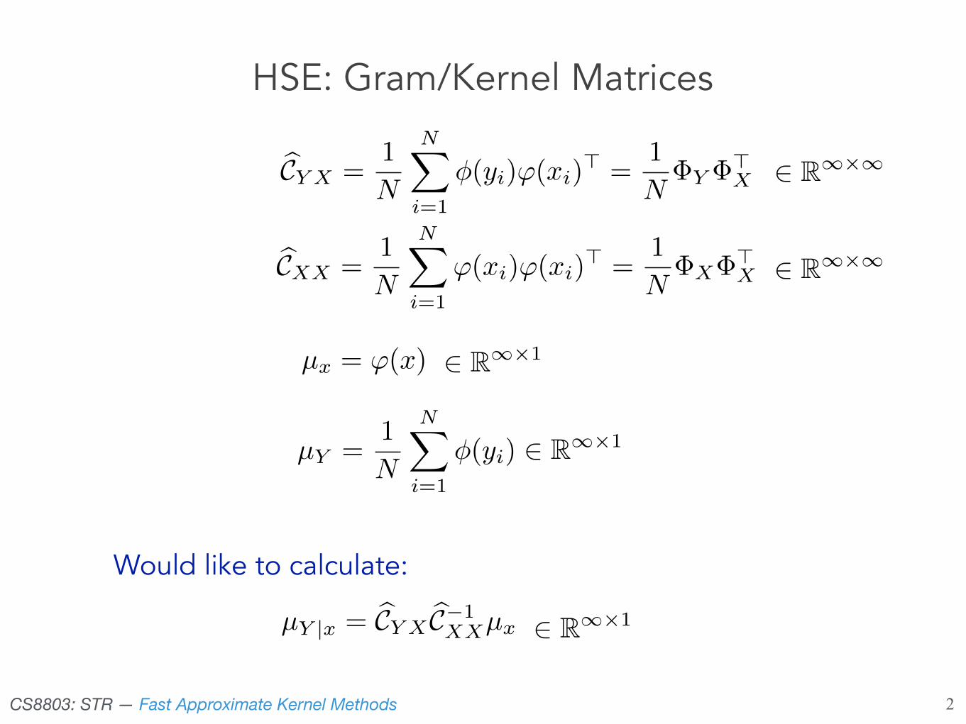
HSE: Gram/Kernel Matrices
bCY X =1
N
NX
i=1
�(yi)'(xi)> =
1
N
�Y �>X 2 R1⇥1
2 R1⇥1
bCXX =1
N
NX
i=1
'(xi)'(xi)> =
1
N
�X�>X 2 R1⇥1
µ
x
= '(x)
µY |x = bC
Y X
bC�1XX
µx
Would like to calculate:
µY =1
N
NX
i=1
�(yi) 2 R1⇥1
2 R1⇥1

CS8803: STR — Fast Approximate Kernel Methods 3
HSE: Gram/Kernel Matrices
µY |x = bC
Y X
bC�1XX
µx
µ̂
Y |x = �Y
�>X
��
X
�>X
+ �I
��1'(x)
GXX =1
N�>
X�X
= �Y (�>X�X + �NI)�1�>
X'(x)
= �Y (GXX + �NI)�1GXX(:, i)
where
2 RN⇥N
2 RN⇥1GXX(:, i) = �>
X'(xi)
(Woodbury) Matrix Inversion Lemma
GXX =1
N�>
X�X
CS8803: STR — Fast Approximate Kernel Methods 4
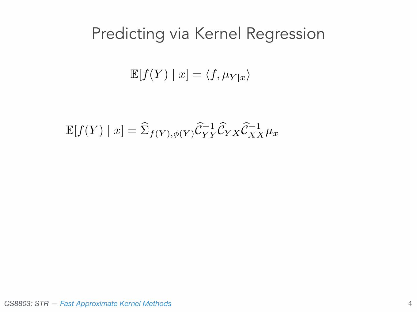
Predicting via Kernel Regression
E[f(Y ) | x] = hf, µY |xi
E[f(Y ) | x] = b⌃f(Y ),�(Y )
bC�1Y Y
bCY X
bC�1XX
µ
x
= b⌃f(Y ),'(X)
bC�1XX
µ
x

CS8803: STR — Fast Approximate Kernel Methods
racetrack
Manuscript under review by AISTATS 2012
0 10 20 30 40 50 60 70 80 90 1000
40
80
120
160A. C.
Prediction Horizon
RMS ErrorIMU
Racetrack
Mean Obs.Slot Car B.
Laplacian Eigenmap
Gaussian RBF
Kalman Filter
LinearHSE-HMMManifold-HMM
HMM (EM)Previous Obs.
Car Locations Predicted by
Different State Spaces
Figure 3: Slot car with inertial measurement unit (IMU). (A) The slot car platform: the car and IMU (top) andracetrack (bottom). (B) A comparison of training data embedded into the state space of three di�erent learnedmodels. Red line indicates true 2-d position of the car over time, blue lines indicate the prediction from statespace. The top graph shows the Kalman filter state space (linear kernel), the middle graph shows the HSE-HMM state space (Gaussian RBF kernel), and the bottom graph shows the manifold HSE-HMM state space(LE kernel). The LE kernel finds the best representation of the true manifold. (C) Root mean squared error forprediction (averaged over 250 trials) with di�erent estimated models. The HSE-HMM significantly outperformsthe other learned models by taking advantage of the fact that the data we want to predict lies on a manifold.
structing a manifold, none of these papers comparesthe predictive accuracy of its model to state-of-the-artdynamical system identification algorithms.
7 Conclusion
In this paper we propose a class of problems calledtwo-manifold problems where two sets of correspond-ing data points, generated by a single latent manifold,lie on or near two di�erent higher dimensional mani-folds. We design algorithms by relating two-manifoldproblems to cross-covariance operators in RKHS, andshow that these algorithms result in a significant im-provement over standard manifold learning approachesin the presence of noise. This is an appealing result:manifold learning algorithms typically assume that ob-servations are (close to) noiseless, an assumption thatis rarely satisfied in practice.
Furthermore, we demonstrate the utility of two-manifold problems by extending a recent dynamicalsystem identification algorithm to learn a system witha state space that lies on a manifold. The resulting al-gorithm learns a model that outperforms the currentstate-of-the-art in terms of predictive accuracy. To ourknowledge this is the first combination of system iden-tification and manifold learning that accurately iden-tifies a latent time series manifold and is competitivewith the best system identification algorithms at learn-ing accurate models.
Hilbert Space Embeddings of Hidden Markov Models
A. B.
0 10 20 30 40 50 60 70 80 90 100
3
4
5
6
7
8x 10⁶
Prediction Horizon
Avg. P
redic
tion E
rr.
2
1
IMUSlo
t C
ar
0
Racetrack
RR-HMMLDS
HMMMeanLast
Embedded
Figure 4. Slot car inertial measurement data. (A) The slotcar platform and the IMU (top) and the racetrack (bot-tom). (B) Squared error for prediction with di�erent esti-mated models and baselines.
this data while the slot car circled the track controlledby a constant policy. The goal of this experiment wasto learn a model of the noisy IMU data, and, afterfiltering, to predict future IMU readings.
We trained a 20-dimensional embedded HMM usingAlgorithm 1 with sequences of 150 consecutive obser-vations (Section 3.8). The bandwidth parameter ofthe Gaussian RBF kernels is set with ‘median trick’.The regularization parameter � is set of 10�4. Forcomparison, a 20-dimensional RR-HMM with Parzenwindows is learned also with sequences of 150 observa-tions; a 20-dimensional LDS is learned using SubspaceID with Hankel matrices of 150 time steps; and finally,a 20-state discrete HMM (with 400 level of discretiza-tion for observations) is learned using EM algorithmrun until convergence.
For each model, we performed filtering for di�erentextents t1 = 100, 101, . . . , 250, then predicted an im-age which was a further t2 steps in the future, fort2 = 1, 2..., 100. The squared error of this predictionin the IMU’s measurement space was recorded, andaveraged over all the di�erent filtering extents t1 toobtain means which are plotted in Figure 4(B). Againthe embedded HMM learned by the kernel spectral al-gorithm yields lower prediction error compared to eachof the alternatives consistently for the duration of theprediction horizon.
4.3. Audio Event ClassificationOur final experiment concerns an audio classificationtask. The data, recently presented in (Ramos et al.,2010), consisted of sequences of 13-dimensional Mel-Frequency Cepstral Coe⇥cients (MFCC) obtainedfrom short clips of raw audio data recorded usinga portable sensor device. Six classes of labeled au-dio clips were present in the data, one being HumanSpeech. For this experiment we grouped the latter fiveclasses into a single class of Non-human sounds to for-mulate a binary Human vs. Non-human classificationtask. Since the original data had a disproportionatelylarge amount of Human Speech samples, this groupingresulted in a more balanced dataset with 40 minutes
Latent Space Dimensionality
Acc
ura
cy (
%)
HMM
LDS
RR!HMM
Embedded
10 20 30 40 5060
70
80
90
85
75
65
Figure 5. Accuracies and 95% confidence intervals for Hu-man vs. Non-human audio event classification, comparingembedded HMMs to other common sequential models atdi�erent latent state space sizes.
11 seconds of Human and 28 minutes 43 seconds ofNon-human audio data. To reduce noise and trainingtime we averaged the data every 100 timesteps (corre-sponding to 1 second) and downsampled.
For each of the two classes, we trained embeddedHMMs with 10, 20, . . . , 50 latent dimensions usingspectral learning and Gaussian RBF kernels withbandwidth set with the ‘median trick’. The regulariza-tion parameter � is set at 10�1. For e⇥ciency we usedrandom features for approximating the kernel (Rahimi& Recht, 2008). For comparison, regular HMMs withaxis-aligned Gaussian observation models, LDSs andRR-HMMs were trained using multi-restart EM (toavoid local minima), stable Subspace ID and the spec-tral algorithm of (Siddiqi et al., 2009) respectively, alsowith 10, . . . , 50 latent dimensions or states.
For RR-HMMs, regular HMMs and LDSs, the class-conditional data sequence likelihood is the scoringfunction for classification. For embedded HMMs, thescoring function for a test sequence x1:t is the log ofthe product of the compatibility scores for each obser-vation, i.e.
⇧t�=1 log
�⇤⇥(x� ), µ̂X� |x1:��1
⌅F
⇥.
For each model size, we performed 50 random 2:1partitions of data from each class and used the re-sulting datasets for training and testing respectively.The mean accuracy and 95% confidence intervals overthese 50 randomizations are reported in Figure 5. Thegraph indicates that embedded HMMs have higher ac-curacy and lower variance than other standard alter-natives at every model size. Though other learningalgorithms for HMMs and LDSs exist, our experimentshows this to be a non-trivial sequence classificationproblem where embedded HMMs significantly outper-form commonly used sequential models trained usingtypical learning and model selection methods.
5. Conclusion
We proposed a Hilbert space embedding of HMMsthat extends traditional HMMs to structured and non-Gaussian continuous observation distributions. The
Hilbert Space Embeddings of Hidden Markov Models
A. B.
0 10 20 30 40 50 60 70 80 90 100
3
4
5
6
7
8x 10⁶
Prediction Horizon
Av
g.
Pre
dic
tio
n E
rr.
2
1
IMUSlo
t C
ar
0
Racetrack
RR-HMMLDS
HMMMeanLast
Embedded
Figure 4. Slot car inertial measurement data. (A) The slotcar platform and the IMU (top) and the racetrack (bot-tom). (B) Squared error for prediction with di�erent esti-mated models and baselines.
this data while the slot car circled the track controlledby a constant policy. The goal of this experiment wasto learn a model of the noisy IMU data, and, afterfiltering, to predict future IMU readings.
We trained a 20-dimensional embedded HMM usingAlgorithm 1 with sequences of 150 consecutive obser-vations (Section 3.8). The bandwidth parameter ofthe Gaussian RBF kernels is set with ‘median trick’.The regularization parameter � is set of 10�4. Forcomparison, a 20-dimensional RR-HMM with Parzenwindows is learned also with sequences of 150 observa-tions; a 20-dimensional LDS is learned using SubspaceID with Hankel matrices of 150 time steps; and finally,a 20-state discrete HMM (with 400 level of discretiza-tion for observations) is learned using EM algorithmrun until convergence.
For each model, we performed filtering for di�erentextents t1 = 100, 101, . . . , 250, then predicted an im-age which was a further t2 steps in the future, fort2 = 1, 2..., 100. The squared error of this predictionin the IMU’s measurement space was recorded, andaveraged over all the di�erent filtering extents t1 toobtain means which are plotted in Figure 4(B). Againthe embedded HMM learned by the kernel spectral al-gorithm yields lower prediction error compared to eachof the alternatives consistently for the duration of theprediction horizon.
4.3. Audio Event ClassificationOur final experiment concerns an audio classificationtask. The data, recently presented in (Ramos et al.,2010), consisted of sequences of 13-dimensional Mel-Frequency Cepstral Coe⇥cients (MFCC) obtainedfrom short clips of raw audio data recorded usinga portable sensor device. Six classes of labeled au-dio clips were present in the data, one being HumanSpeech. For this experiment we grouped the latter fiveclasses into a single class of Non-human sounds to for-mulate a binary Human vs. Non-human classificationtask. Since the original data had a disproportionatelylarge amount of Human Speech samples, this groupingresulted in a more balanced dataset with 40 minutes
Latent Space Dimensionality
Acc
ura
cy (
%)
HMM
LDS
RR!HMM
Embedded
10 20 30 40 5060
70
80
90
85
75
65
Figure 5. Accuracies and 95% confidence intervals for Hu-man vs. Non-human audio event classification, comparingembedded HMMs to other common sequential models atdi�erent latent state space sizes.
11 seconds of Human and 28 minutes 43 seconds ofNon-human audio data. To reduce noise and trainingtime we averaged the data every 100 timesteps (corre-sponding to 1 second) and downsampled.
For each of the two classes, we trained embeddedHMMs with 10, 20, . . . , 50 latent dimensions usingspectral learning and Gaussian RBF kernels withbandwidth set with the ‘median trick’. The regulariza-tion parameter � is set at 10�1. For e⇥ciency we usedrandom features for approximating the kernel (Rahimi& Recht, 2008). For comparison, regular HMMs withaxis-aligned Gaussian observation models, LDSs andRR-HMMs were trained using multi-restart EM (toavoid local minima), stable Subspace ID and the spec-tral algorithm of (Siddiqi et al., 2009) respectively, alsowith 10, . . . , 50 latent dimensions or states.
For RR-HMMs, regular HMMs and LDSs, the class-conditional data sequence likelihood is the scoringfunction for classification. For embedded HMMs, thescoring function for a test sequence x1:t is the log ofthe product of the compatibility scores for each obser-vation, i.e.
⇧t�=1 log
�⇤⇥(x� ), µ̂X� |x1:��1
⌅F
⇥.
For each model size, we performed 50 random 2:1partitions of data from each class and used the re-sulting datasets for training and testing respectively.The mean accuracy and 95% confidence intervals overthese 50 randomizations are reported in Figure 5. Thegraph indicates that embedded HMMs have higher ac-curacy and lower variance than other standard alter-natives at every model size. Though other learningalgorithms for HMMs and LDSs exist, our experimentshows this to be a non-trivial sequence classificationproblem where embedded HMMs significantly outper-form commonly used sequential models trained usingtypical learning and model selection methods.
5. Conclusion
We proposed a Hilbert space embedding of HMMsthat extends traditional HMMs to structured and non-Gaussian continuous observation distributions. The
5
Example: Slotcar Position Estimation
0 50 100 150−3
−2
−1
0
1
2
3 x10³
E[f(Y ) | x] = hf, µY |xi

CS8803: STR — Fast Approximate Kernel Methods 6
Predicting via Kernel Regression
E[f(Y ) | x] = hf, µY |xi
E[f(Y ) | x] = b⌃f(Y ),�(Y )
bC�1Y Y
bCY X
bC�1XX
µ
x
= b⌃f(Y ),'(X)
bC�1XX
µ
x
f(Y )(GXX + �NI)�1GXX(:, i)
µ̂
Y |x = �Y
�>X
��
X
�>X
+ �I
��1'(x)f(Y )�>
Y (�Y �>Y + �I)�1
f(Y )(�>Y �Y + �I)�1�>
Y �Y (�>X�X + �I)�1�>
X'(x)

CS8803: STR — Fast Approximate Kernel Methods
racetrack
Manuscript under review by AISTATS 2012
0 10 20 30 40 50 60 70 80 90 1000
40
80
120
160A. C.
Prediction Horizon
RMS ErrorIMU
Racetrack
Mean Obs.Slot Car B.
Laplacian Eigenmap
Gaussian RBF
Kalman Filter
LinearHSE-HMMManifold-HMM
HMM (EM)Previous Obs.
Car Locations Predicted by
Different State Spaces
Figure 3: Slot car with inertial measurement unit (IMU). (A) The slot car platform: the car and IMU (top) andracetrack (bottom). (B) A comparison of training data embedded into the state space of three di�erent learnedmodels. Red line indicates true 2-d position of the car over time, blue lines indicate the prediction from statespace. The top graph shows the Kalman filter state space (linear kernel), the middle graph shows the HSE-HMM state space (Gaussian RBF kernel), and the bottom graph shows the manifold HSE-HMM state space(LE kernel). The LE kernel finds the best representation of the true manifold. (C) Root mean squared error forprediction (averaged over 250 trials) with di�erent estimated models. The HSE-HMM significantly outperformsthe other learned models by taking advantage of the fact that the data we want to predict lies on a manifold.
structing a manifold, none of these papers comparesthe predictive accuracy of its model to state-of-the-artdynamical system identification algorithms.
7 Conclusion
In this paper we propose a class of problems calledtwo-manifold problems where two sets of correspond-ing data points, generated by a single latent manifold,lie on or near two di�erent higher dimensional mani-folds. We design algorithms by relating two-manifoldproblems to cross-covariance operators in RKHS, andshow that these algorithms result in a significant im-provement over standard manifold learning approachesin the presence of noise. This is an appealing result:manifold learning algorithms typically assume that ob-servations are (close to) noiseless, an assumption thatis rarely satisfied in practice.
Furthermore, we demonstrate the utility of two-manifold problems by extending a recent dynamicalsystem identification algorithm to learn a system witha state space that lies on a manifold. The resulting al-gorithm learns a model that outperforms the currentstate-of-the-art in terms of predictive accuracy. To ourknowledge this is the first combination of system iden-tification and manifold learning that accurately iden-tifies a latent time series manifold and is competitivewith the best system identification algorithms at learn-ing accurate models.
Hilbert Space Embeddings of Hidden Markov Models
A. B.
0 10 20 30 40 50 60 70 80 90 100
3
4
5
6
7
8x 10⁶
Prediction Horizon
Avg. P
redic
tion E
rr.
2
1
IMUSlo
t C
ar
0
Racetrack
RR-HMMLDS
HMMMeanLast
Embedded
Figure 4. Slot car inertial measurement data. (A) The slotcar platform and the IMU (top) and the racetrack (bot-tom). (B) Squared error for prediction with di�erent esti-mated models and baselines.
this data while the slot car circled the track controlledby a constant policy. The goal of this experiment wasto learn a model of the noisy IMU data, and, afterfiltering, to predict future IMU readings.
We trained a 20-dimensional embedded HMM usingAlgorithm 1 with sequences of 150 consecutive obser-vations (Section 3.8). The bandwidth parameter ofthe Gaussian RBF kernels is set with ‘median trick’.The regularization parameter � is set of 10�4. Forcomparison, a 20-dimensional RR-HMM with Parzenwindows is learned also with sequences of 150 observa-tions; a 20-dimensional LDS is learned using SubspaceID with Hankel matrices of 150 time steps; and finally,a 20-state discrete HMM (with 400 level of discretiza-tion for observations) is learned using EM algorithmrun until convergence.
For each model, we performed filtering for di�erentextents t1 = 100, 101, . . . , 250, then predicted an im-age which was a further t2 steps in the future, fort2 = 1, 2..., 100. The squared error of this predictionin the IMU’s measurement space was recorded, andaveraged over all the di�erent filtering extents t1 toobtain means which are plotted in Figure 4(B). Againthe embedded HMM learned by the kernel spectral al-gorithm yields lower prediction error compared to eachof the alternatives consistently for the duration of theprediction horizon.
4.3. Audio Event ClassificationOur final experiment concerns an audio classificationtask. The data, recently presented in (Ramos et al.,2010), consisted of sequences of 13-dimensional Mel-Frequency Cepstral Coe⇥cients (MFCC) obtainedfrom short clips of raw audio data recorded usinga portable sensor device. Six classes of labeled au-dio clips were present in the data, one being HumanSpeech. For this experiment we grouped the latter fiveclasses into a single class of Non-human sounds to for-mulate a binary Human vs. Non-human classificationtask. Since the original data had a disproportionatelylarge amount of Human Speech samples, this groupingresulted in a more balanced dataset with 40 minutes
Latent Space Dimensionality
Acc
ura
cy (
%)
HMM
LDS
RR!HMM
Embedded
10 20 30 40 5060
70
80
90
85
75
65
Figure 5. Accuracies and 95% confidence intervals for Hu-man vs. Non-human audio event classification, comparingembedded HMMs to other common sequential models atdi�erent latent state space sizes.
11 seconds of Human and 28 minutes 43 seconds ofNon-human audio data. To reduce noise and trainingtime we averaged the data every 100 timesteps (corre-sponding to 1 second) and downsampled.
For each of the two classes, we trained embeddedHMMs with 10, 20, . . . , 50 latent dimensions usingspectral learning and Gaussian RBF kernels withbandwidth set with the ‘median trick’. The regulariza-tion parameter � is set at 10�1. For e⇥ciency we usedrandom features for approximating the kernel (Rahimi& Recht, 2008). For comparison, regular HMMs withaxis-aligned Gaussian observation models, LDSs andRR-HMMs were trained using multi-restart EM (toavoid local minima), stable Subspace ID and the spec-tral algorithm of (Siddiqi et al., 2009) respectively, alsowith 10, . . . , 50 latent dimensions or states.
For RR-HMMs, regular HMMs and LDSs, the class-conditional data sequence likelihood is the scoringfunction for classification. For embedded HMMs, thescoring function for a test sequence x1:t is the log ofthe product of the compatibility scores for each obser-vation, i.e.
⇧t�=1 log
�⇤⇥(x� ), µ̂X� |x1:��1
⌅F
⇥.
For each model size, we performed 50 random 2:1partitions of data from each class and used the re-sulting datasets for training and testing respectively.The mean accuracy and 95% confidence intervals overthese 50 randomizations are reported in Figure 5. Thegraph indicates that embedded HMMs have higher ac-curacy and lower variance than other standard alter-natives at every model size. Though other learningalgorithms for HMMs and LDSs exist, our experimentshows this to be a non-trivial sequence classificationproblem where embedded HMMs significantly outper-form commonly used sequential models trained usingtypical learning and model selection methods.
5. Conclusion
We proposed a Hilbert space embedding of HMMsthat extends traditional HMMs to structured and non-Gaussian continuous observation distributions. The
Hilbert Space Embeddings of Hidden Markov Models
A. B.
0 10 20 30 40 50 60 70 80 90 100
3
4
5
6
7
8x 10⁶
Prediction Horizon
Av
g.
Pre
dic
tio
n E
rr.
2
1
IMUSlo
t C
ar
0
Racetrack
RR-HMMLDS
HMMMeanLast
Embedded
Figure 4. Slot car inertial measurement data. (A) The slotcar platform and the IMU (top) and the racetrack (bot-tom). (B) Squared error for prediction with di�erent esti-mated models and baselines.
this data while the slot car circled the track controlledby a constant policy. The goal of this experiment wasto learn a model of the noisy IMU data, and, afterfiltering, to predict future IMU readings.
We trained a 20-dimensional embedded HMM usingAlgorithm 1 with sequences of 150 consecutive obser-vations (Section 3.8). The bandwidth parameter ofthe Gaussian RBF kernels is set with ‘median trick’.The regularization parameter � is set of 10�4. Forcomparison, a 20-dimensional RR-HMM with Parzenwindows is learned also with sequences of 150 observa-tions; a 20-dimensional LDS is learned using SubspaceID with Hankel matrices of 150 time steps; and finally,a 20-state discrete HMM (with 400 level of discretiza-tion for observations) is learned using EM algorithmrun until convergence.
For each model, we performed filtering for di�erentextents t1 = 100, 101, . . . , 250, then predicted an im-age which was a further t2 steps in the future, fort2 = 1, 2..., 100. The squared error of this predictionin the IMU’s measurement space was recorded, andaveraged over all the di�erent filtering extents t1 toobtain means which are plotted in Figure 4(B). Againthe embedded HMM learned by the kernel spectral al-gorithm yields lower prediction error compared to eachof the alternatives consistently for the duration of theprediction horizon.
4.3. Audio Event ClassificationOur final experiment concerns an audio classificationtask. The data, recently presented in (Ramos et al.,2010), consisted of sequences of 13-dimensional Mel-Frequency Cepstral Coe⇥cients (MFCC) obtainedfrom short clips of raw audio data recorded usinga portable sensor device. Six classes of labeled au-dio clips were present in the data, one being HumanSpeech. For this experiment we grouped the latter fiveclasses into a single class of Non-human sounds to for-mulate a binary Human vs. Non-human classificationtask. Since the original data had a disproportionatelylarge amount of Human Speech samples, this groupingresulted in a more balanced dataset with 40 minutes
Latent Space Dimensionality
Acc
ura
cy (
%)
HMM
LDS
RR!HMM
Embedded
10 20 30 40 5060
70
80
90
85
75
65
Figure 5. Accuracies and 95% confidence intervals for Hu-man vs. Non-human audio event classification, comparingembedded HMMs to other common sequential models atdi�erent latent state space sizes.
11 seconds of Human and 28 minutes 43 seconds ofNon-human audio data. To reduce noise and trainingtime we averaged the data every 100 timesteps (corre-sponding to 1 second) and downsampled.
For each of the two classes, we trained embeddedHMMs with 10, 20, . . . , 50 latent dimensions usingspectral learning and Gaussian RBF kernels withbandwidth set with the ‘median trick’. The regulariza-tion parameter � is set at 10�1. For e⇥ciency we usedrandom features for approximating the kernel (Rahimi& Recht, 2008). For comparison, regular HMMs withaxis-aligned Gaussian observation models, LDSs andRR-HMMs were trained using multi-restart EM (toavoid local minima), stable Subspace ID and the spec-tral algorithm of (Siddiqi et al., 2009) respectively, alsowith 10, . . . , 50 latent dimensions or states.
For RR-HMMs, regular HMMs and LDSs, the class-conditional data sequence likelihood is the scoringfunction for classification. For embedded HMMs, thescoring function for a test sequence x1:t is the log ofthe product of the compatibility scores for each obser-vation, i.e.
⇧t�=1 log
�⇤⇥(x� ), µ̂X� |x1:��1
⌅F
⇥.
For each model size, we performed 50 random 2:1partitions of data from each class and used the re-sulting datasets for training and testing respectively.The mean accuracy and 95% confidence intervals overthese 50 randomizations are reported in Figure 5. Thegraph indicates that embedded HMMs have higher ac-curacy and lower variance than other standard alter-natives at every model size. Though other learningalgorithms for HMMs and LDSs exist, our experimentshows this to be a non-trivial sequence classificationproblem where embedded HMMs significantly outper-form commonly used sequential models trained usingtypical learning and model selection methods.
5. Conclusion
We proposed a Hilbert space embedding of HMMsthat extends traditional HMMs to structured and non-Gaussian continuous observation distributions. The
7
Example: Slotcar Position Estimation
0 50 100 150−3
−2
−1
0
1
2
3 x10³
E[f(Y ) | x] = hf, µY |xi
CS8803: STR — Fast Approximate Kernel Methods 8
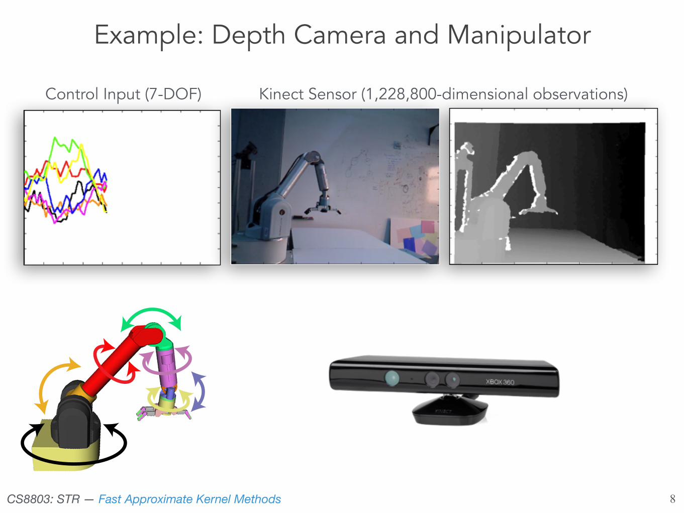
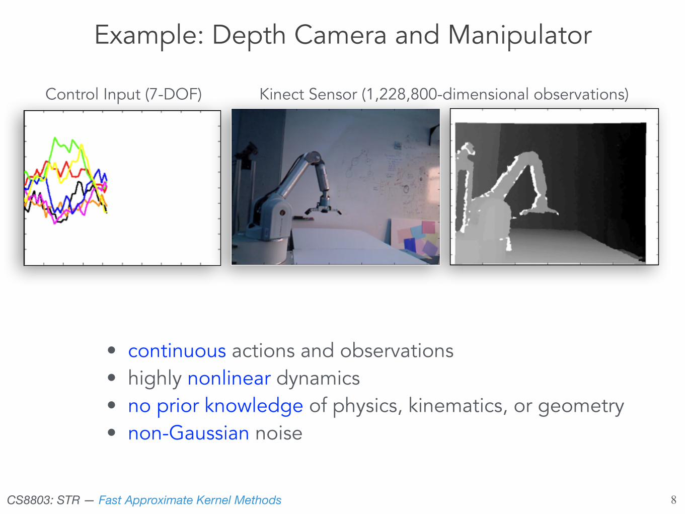
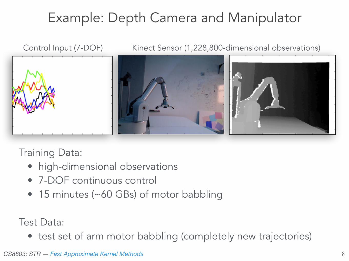
Control Input (7-DOF) Kinect Sensor (1,228,800-dimensional observations)
Example: Depth Camera and Manipulator

CS8803: STR — Fast Approximate Kernel Methods 8
Control Input (7-DOF) Kinect Sensor (1,228,800-dimensional observations)
The Challenge: learn a full generative model
Example: Depth Camera and Manipulator
CS8803: STR — Fast Approximate Kernel Methods 8
Control Input (7-DOF) Kinect Sensor (1,228,800-dimensional observations)
• continuous actions and observations • highly nonlinear dynamics • no prior knowledge of physics, kinematics, or geometry • non-Gaussian noise
Example: Depth Camera and Manipulator
CS8803: STR — Fast Approximate Kernel Methods 8
Control Input (7-DOF) Kinect Sensor (1,228,800-dimensional observations)
Training Data: • high-dimensional observations • 7-DOF continuous control • 15 minutes (~60 GBs) of motor babbling
Test Data: • test set of arm motor babbling (completely new trajectories)
Example: Depth Camera and Manipulator

CS8803: STR — Fast Approximate Kernel Methods 9
True ObservationPrediction (4 seconds):Filtering (tracking): E[ot | a1:t, o1:t�1] E[ot+120 | a1:t+120, o1:t�1] ot+120
Example: Depth Camera and Manipulator
CS8803: STR — Fast Approximate Kernel Methods 10
CS8803: Statistical Techniques in RoboticsByron Boots
Fast Approximate Kernel Methods
CS8803: STR — Fast Approximate Kernel Methods 11
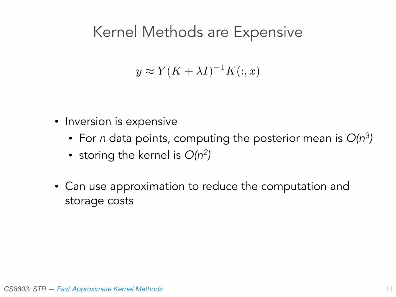
Kernel Methods are Expensive
y ⇡ Y (K + �I)�1K(:, x)
• Inversion is expensive • For n data points, computing the posterior mean is O(n3) • storing the kernel is O(n2)
• Can use approximation to reduce the computation and storage costs

CS8803: STR — Fast Approximate Kernel Methods 12
Methods for Approximating Kernel Machines
• Factorize the Kernel Matrix
• Random Features
• (Random or Greedy) Subset of Data
CS8803: STR — Fast Approximate Kernel Methods 13
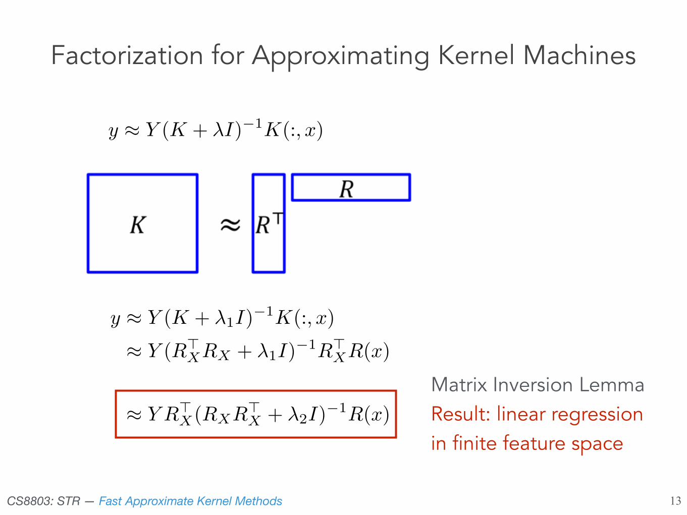
y ⇡ Y (K + �I)�1K(:, x)
Factorization for Approximating Kernel Machines
y ⇡ Y (K + �1I)�1
K(:, x)
⇡ Y (R>XRX + �1I)
�1R
>XR(x)
⇡ Y R
>X(RXR
>X + �2I)
�1R(x)
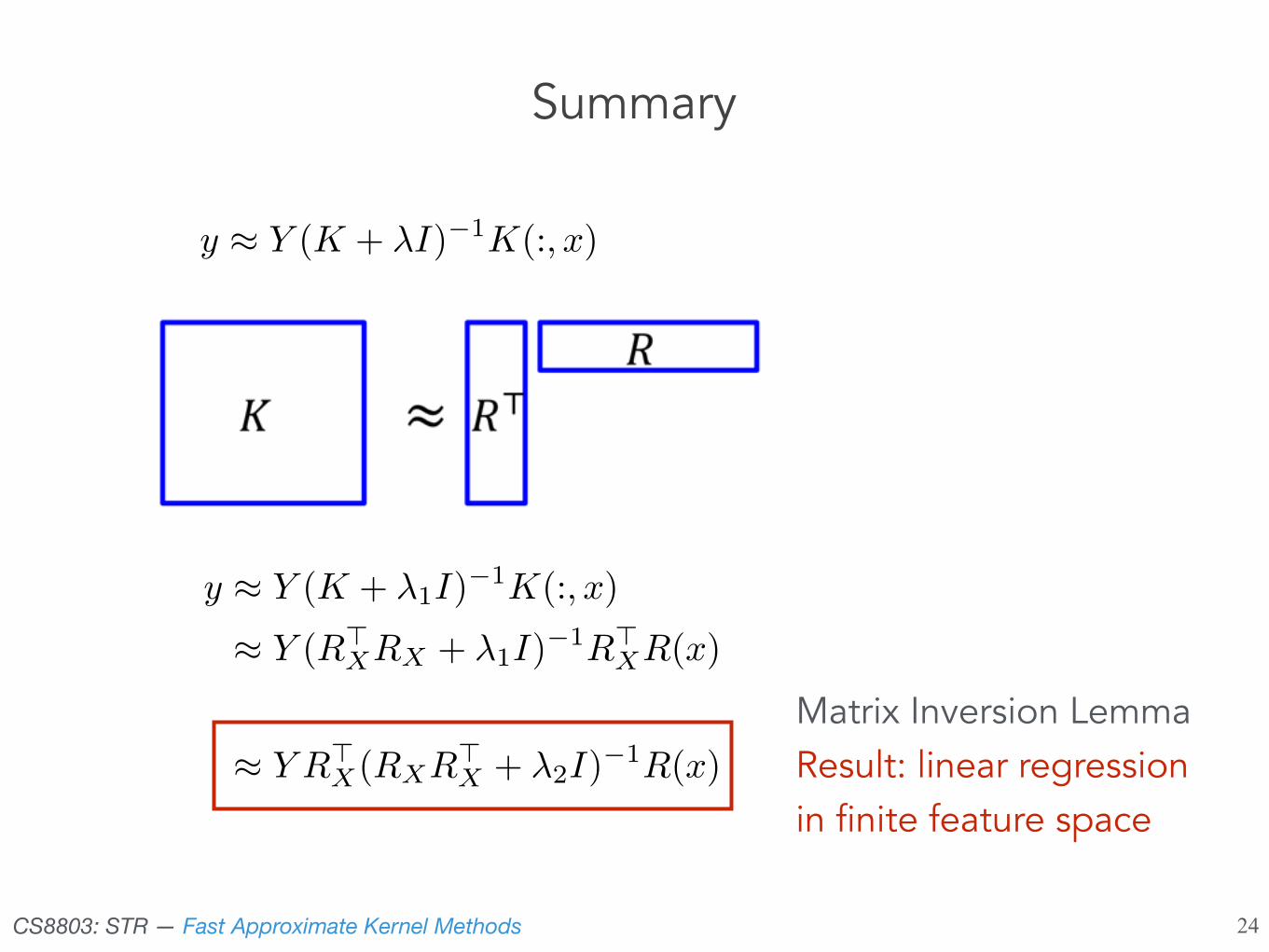
Matrix Inversion Lemma Result: linear regression in finite feature space
CS8803: STR — Fast Approximate Kernel Methods 14
Factorization for Approximating Kernel Machines
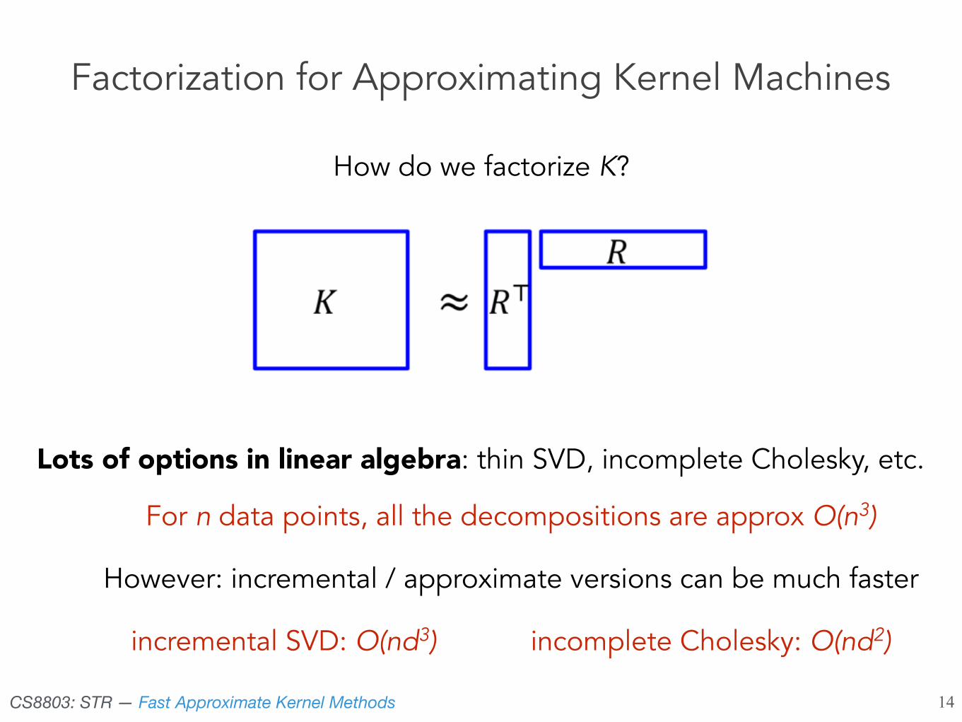
How do we factorize K?
Lots of options in linear algebra: thin SVD, incomplete Cholesky, etc.
For n data points, all the decompositions are approx O(n3)
However: incremental / approximate versions can be much faster
incremental SVD: O(nd3) incomplete Cholesky: O(nd2)
CS8803: STR — Fast Approximate Kernel Methods 15
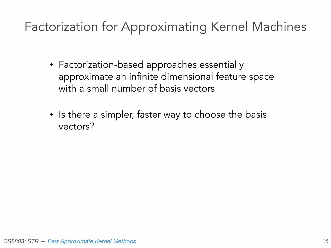
• Factorization-based approaches essentially approximate an infinite dimensional feature space with a small number of basis vectors
• Is there a simpler, faster way to choose the basis vectors?
Factorization for Approximating Kernel Machines

CS8803: STR — Fast Approximate Kernel Methods 16
Methods for Approximating Kernel Machines
• Factorize the Kernel Matrix
• Random Features
• (Random or Greedy) Subset of Data
CS8803: STR — Fast Approximate Kernel Methods 17
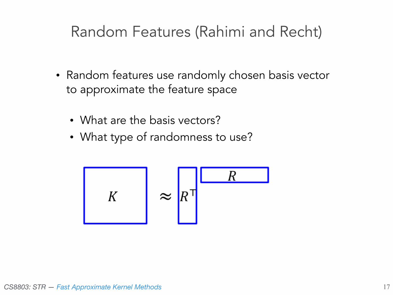
• Random features use randomly chosen basis vector to approximate the feature space
• What are the basis vectors? • What type of randomness to use?
Random Features (Rahimi and Recht)

CS8803: STR — Fast Approximate Kernel Methods 18
Shift Invariant Kernels
• Kernel value only depends on the difference between two data points
• !(",#) =!("−#) =!(Δ)
• A shift invariant kernel !(Δ) is the Fourier transformation of a non-negative measure
• Eg.
CS8803: STR — Fast Approximate Kernel Methods 19
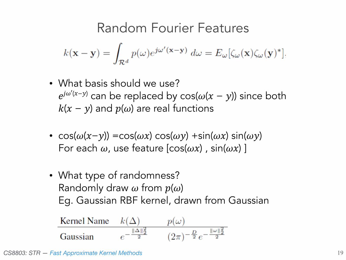
• What basis should we use? $%&′("−#) can be replaced by cos(&(" − #)) since both !(" − #) and ((&) are real functions
• cos(&("−#)) =cos(&") cos(&#) +sin(&") sin(&#) For each &, use feature [cos(&") , sin(&") ]
• What type of randomness? Randomly draw & from ((&)Eg. Gaussian RBF kernel, drawn from Gaussian
Random Fourier Features
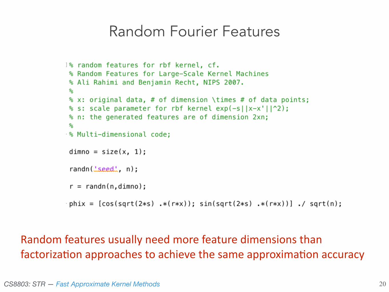
CS8803: STR — Fast Approximate Kernel Methods 20
Random'features'usually'need'more'feature'dimensions'than'factoriza4on'approaches'to'achieve'the'same'approxima4on'accuracy
Random Fourier Features
CS8803: STR — Fast Approximate Kernel Methods 21
Methods for Approximating Kernel Machines
• Factorize the Kernel Matrix
• Random Features
• (Random or Greedy) Subsets of Data
CS8803: STR — Fast Approximate Kernel Methods 22
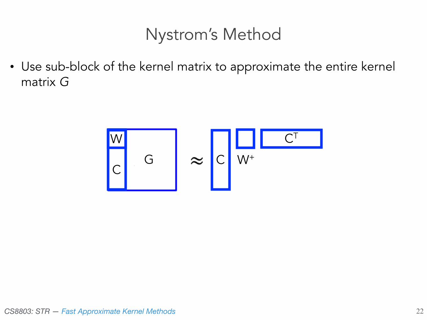
Nystrom’s Method
• Use sub-block of the kernel matrix to approximate the entire kernel matrix G
C W+
CT
C
W
G

CS8803: STR — Fast Approximate Kernel Methods 23
Nystrom’s Method
• Use sub-block of the kernel matrix to approximate the entire kernel matrix G
CS8803: STR — Fast Approximate Kernel Methods 24
Summary
y ⇡ Y (K + �I)�1K(:, x)
y ⇡ Y (K + �1I)�1
K(:, x)
⇡ Y (R>XRX + �1I)
�1R
>XR(x)
⇡ Y R
>X(RXR
>X + �2I)
�1R(x)
Matrix Inversion Lemma Result: linear regression in finite feature space