CS105 - Final Project

Demand Prediction Model for Rental Bicycle Services Jan Raphael Floro | Yunong Louisa Gan | Dan Liu

Demand Prediction Model for Rental Bicycle Services

Final Project Report

Final Version

Fall 2014 • CS105 • Professor David G. Sullivan, Ph.D.

1 Fall 2014 • CS105 • Floro / Liu / Gan

Abstract This project aims to create a numeric estimation for rental bicycles given some key conditions and attributes. A dataset containing past information on the demand for the rental bicycles along with attributes such as weather, temperature, humidity, wind speed, season, month and day of the week was obtained to train and test a number of data mining algorithms and, ultimately, to develop the best possible model for this dataset. Before applying any data mining algorithm, the dataset needed to be processed and examined. The team developed two Python-based programs to automate key preprocessing procedures that the team saw fit to conduct. The dataset was also examined initially through SQL queries to provide a brief analysis on the historical trend of rental bike demands. Finally, a numeric estimation model was developed and a conclusion to the model was formulated.

Authors

Jan Raphael S. Floro Undergraduate – Finance, Management Information Systems Boston University School of Management Boston, MA (617) 682-6579 | [email protected]

Dan Liu Ph.D. Student – Department of Operations & Technology Management Boston University Graduate School of Management Boston, MA (617) 631-6954 | [email protected]

Yunong Louisa Gan Undergraduate Boston University College of Arts & Science Boston, MA (xxx) xxx-xxxx | [email protected]

Demand Prediction Model for Rental Bicycle Services 2

Dataset Description The dataset to be used in this project originates from a single, consolidated comma-separated value (CSV) table generated by a previous similar study by Hadi Fanaee-T of the Laboratory of Artificial Intelligence and Decision Support at University of Porto, Portugal. Data presented in this CSV file is a consolidation of three datasets:

1. Capital Bikeshare® System Data http://capitalbikeshare.com/system-data

2. I-Weather® Weather Data

http://i-weather.com/weather

3. United States District of Columbia Department of Human Resources Holiday Schedule http://dchr.dc.gov/page/holiday-schedule

The final, consolidated CSV file to be used in this project is available at: http://archive.ics.uci.edu/ml/datasets/Bike+Sharing+Dataset# and consists of the following attributes, along with their meanings:

Table 1: Attribute Information

Attribute Definition

instant Record index (unique identifier) dteday date (MM/DD/YYYY) season season (1: spring, 2: summer, 3: fall, 4: winter) yr year (0: 2011, 1: 2012) mnth month (1: January, 2: February, 3: June, …, 12: December) holiday holiday (0: no, 1: yes) weekday day of the week (0: Sunday, 1: Monday, …, 6: Saturday) workingday working day (0: no, 1: yes) weathersit discretized weather (1: clear, 2: mist, 3: light snow/rain, 4: rain/ice) temp normalized temperature in Celsius (divided by 41) atemp normalized feeling temperature in Celsius (divided by 50) hum normalized humidity (divided by 100) windspeed normalized wind speed (divided by 67) casual count of non-registered users who rented bicycles registered count of registered users who rented bicycles cnt count of total (casual plus registered) users who rented bicycles

The dataset consist of a total of 731 records/instances gathered in years 2011 and 2012, published in two separate CSV files for each year. This dataset will be processed further by our team, eliminating unwanted attributes and preparing the dataset to be used with Weka.


Dataset Preparation The initial modification we did in the raw dataset was combine the dataset containing data for year 2011 and one that contained 2012 data. To do this, we simply appended all but the labels from the 2012 CSV file to the end of the 2011 CSV file. We did this because separating the data by the year it was taken is irrelevant as our data mining methodology in Weka requires us to use only one CSV file. Any splitting for test and training will be done later on. Before we are able to run models in our dataset (as well as create an SQL Relational Table), we needed to first needed to remove the following problematic attributes:

Table 2: Problematic Attributes Removed

Attribute Reason for Removal

instant Unique identifier; each value is unique for each record dteday Unique identifier; data was taken only once per day yr Irrelevant; only has two values 0 for 2011 and 1 for 2012 holiday Irrelevant and redundant; only few instances of holidays and

repeats the same information as if weekday = 0 (Sunday) or weekday = 6 (Saturday), holiday will be = 1

workingday Redundant; if weekday = 0 (Sunday) or weekday = 6 (Saturday), workingday is 0

casual Redundant; captures same information as cnt attribute but only for those without registered accounts

registered Redundant; captures same information as cnt attribute but only for those with registered accounts

These attributes were removed using a Python program named removeUnwantedRows.py (a text copy is available at Exhibit 1) and is explained in the next subsection. First Python Program We wrote a Python program called removeUnwantedRows.py to remove the aforementioned problematic attributes. This program takes the dataset that contains both 2011 and 2012 data (the one we manually combined to form a consolidated, single CSV file). For each record after the labels in that dataset, we extract only the attributes we want to keep. We did this first by reading the first line which contains the label to remove it the file processing. We ran a loop that for each record we have in the CSV file, initialize a new list that contains the right amount of fields with empty values, assign the attributes we want to keep from the record to the new list, join them to make a string and then print out the result in a new CSV file. Comments are available in the *.py file attached with this document. Once the program has generated a new CSV file containing the attributes that we wish to keep, we will call another function to take that new CSV file and generate a relational SQL database (SQLite). The details of that program will be discussed in the next subsection.


Second Python Program Our second Python program called createTables.py is to be ran after we have generated a new CSV file from removeUnwantedRows.py. This new program will create a database table that is formatted for the attributes we have kept and reads in the new CSV file generated by the first program. The program will read the first line which contains the labels to prevent the labels from being imported to the SQL table. A loop will then be used to read the succeeding lines, convert the line into a list of values to be inserted, and pass that along with a parameterized SQL query template that adds it into the SQL table. Along with values in each line, we have used a counter to generate a unique identifier (primary key) for the SQL table. We have appended the value of the counter in the first index of the list of fields. Comments are available in the *.py file for further disambiguation. The program will output an SQLite file that can be opened with SQLite Manager, a popular Mozilla Firefox extension. We created this SQLite algorithm in an effort to better explain our historical data through queries and data visualization. This analysis is done before running any data mining algorithm from our dataset. The following section will first display our analysis on both the queries we have run (depicting what our dataset looks like in terms of historical facts) and present the various data mining techniques we used and the model that was resulted from each. Note: We will further process the data in Weka, but that processing will be done in the Data Analysis: Numeric Estimation section. The processing discussed in this current section was mainly to remove the unwanted attributes and create the SQL database.


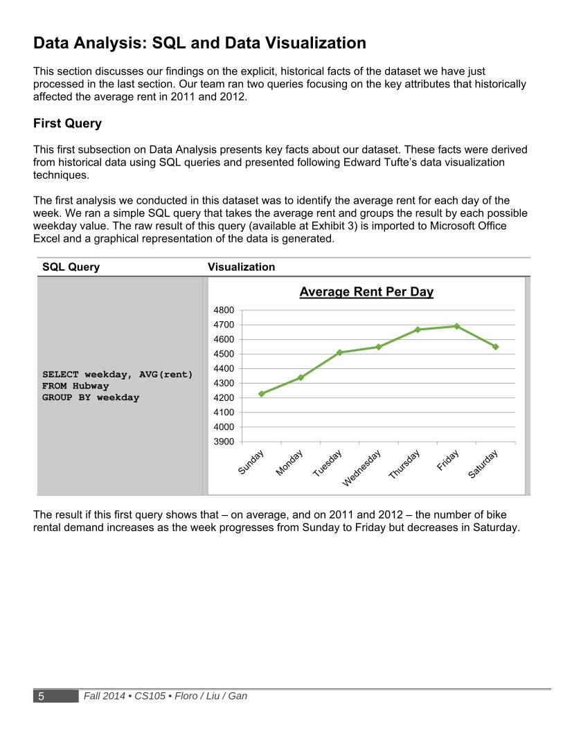
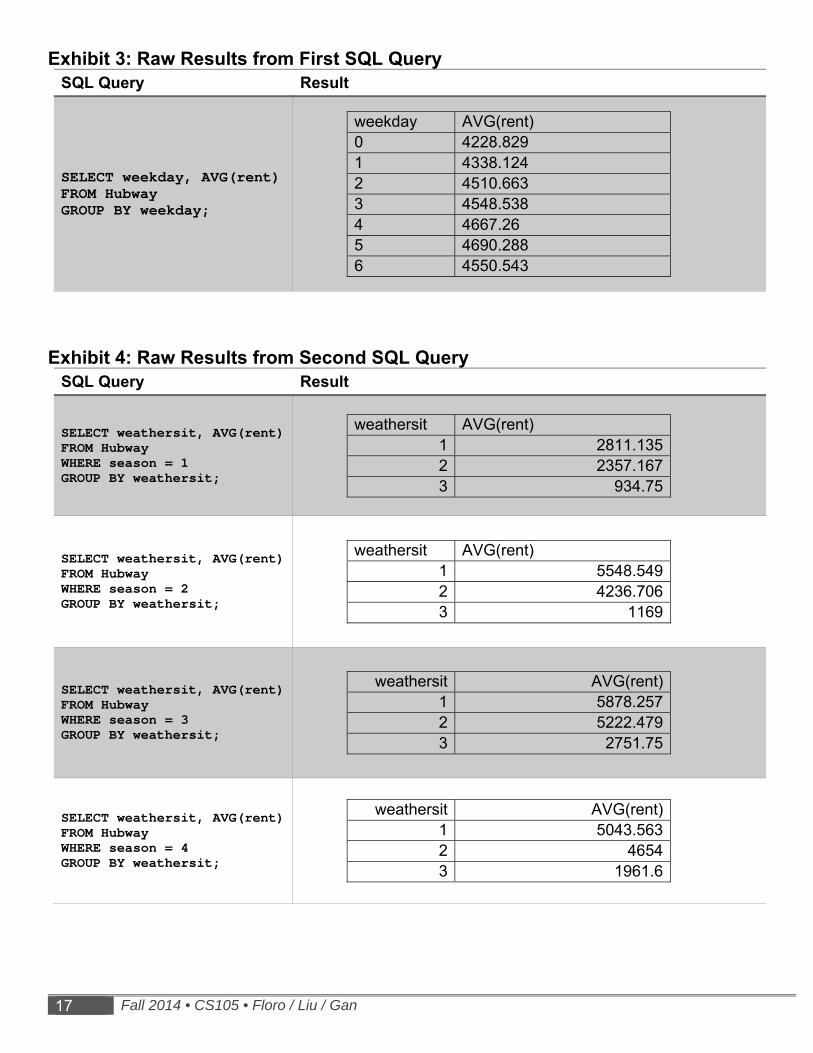
Data Analysis: SQL and Data Visualization This section discusses our findings on the explicit, historical facts of the dataset we have just processed in the last section. Our team ran two queries focusing on the key attributes that historically affected the average rent in 2011 and 2012. First Query This first subsection on Data Analysis presents key facts about our dataset. These facts were derived from historical data using SQL queries and presented following Edward Tufte’s data visualization techniques. The first analysis we conducted in this dataset was to identify the average rent for each day of the week. We ran a simple SQL query that takes the average rent and groups the result by each possible weekday value. The raw result of this query (available at Exhibit 3) is imported to Microsoft Office Excel and a graphical representation of the data is generated.

SQL Query Visualization

SELECT weekday, AVG(rent) FROM Hubway GROUP BY weekday

The result if this first query shows that – on average, and on 2011 and 2012 – the number of bike rental demand increases as the week progresses from Sunday to Friday but decreases in Saturday.

3900

4000

4100

4200

4300

4400

4500

4600

4700

4800

Average Rent Per Day


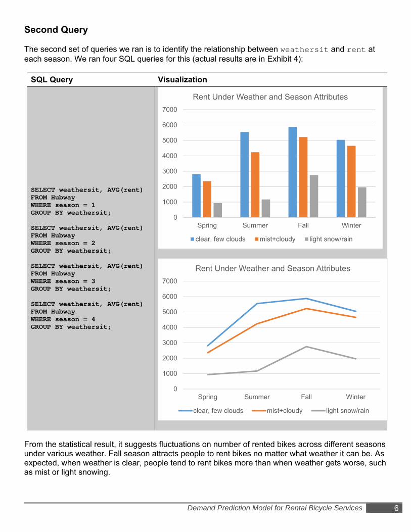
Second Query The second set of queries we ran is to identify the relationship between weathersit and rent at each season. We ran four SQL queries for this (actual results are in Exhibit 4):

SQL Query Visualization

SELECT weathersit, AVG(rent) FROM Hubway WHERE season = 1 GROUP BY weathersit; SELECT weathersit, AVG(rent) FROM Hubway WHERE season = 2 GROUP BY weathersit; SELECT weathersit, AVG(rent) FROM Hubway WHERE season = 3 GROUP BY weathersit; SELECT weathersit, AVG(rent) FROM Hubway WHERE season = 4 GROUP BY weathersit;

From the statistical result, it suggests fluctuations on number of rented bikes across different seasons under various weather. Fall season attracts people to rent bikes no matter what weather it can be. As expected, when weather is clear, people tend to rent bikes more than when weather gets worse, such as mist or light snowing.

0

1000

2000

3000

4000

5000

6000

7000

Spring Summer Fall Winter

Rent Under Weather and Season Attributes

clear, few clouds mist+cloudy light snow/rain

0

1000

2000

3000

4000

5000

6000

7000

Spring Summer Fall Winter

Rent Under Weather and Season Attributes

clear, few clouds mist+cloudy light snow/rain


Data Analysis: Numeric Estimation Data Mining This section is presents our analysis on select data mining algorithms found in Weka (specifically for numeric estimation). Before we display our analysis, the dataset produced in our first Python program (recall that this is a CSV file that has problematic attributes removed from the original, downloaded dataset) must be further processed to ensure fidelity in the Weka software. Weka-specific Preprocessing The purpose of this subsection is to discuss how the data’s attributes were formatted (whether numeric or nominal) and how the dataset was divided for training and testing a model. The prerequisite for this procedure states that the original, downloaded and consolidated dataset (the one that contains the 2011 and 2012 data together) must be processed by removeUnwantedRows.py and must now have a new CSV file without the problematic attributes.

1. Initially, Weka Explorer was opened and the CSV file without problematic attributes was opened

2. The following attributes were converted to Nominal (or made sure they were) due to them having numbers as the input but are really representing codes specified by the dataset authors:

a. season b. mnth c. weekday d. weathersit

These attributes were not continuous and any mathematical operation done on them would not be descriptive. The conversion was done using a built-in Weka feature called “NumericToNominal”

3. The other attributes (temp, atemp, hum, windspeed and cnt) all had numeric type and this should be kept numeric. However, in rare cases that Weka chooses to specify them as nominal, one could simply use another built-in Weka filter called “NominalToNumeric”

4. The dataset now needs to be randomized in order to eliminate any bias found in the order of the data. To do this, a built-in Weka filter called “Randomize” is applied and the dataset is saved as an *.arff file

5. From this randomized ARFF file, the data must now be split for training and testing models, with 80% of the total dataset for training and 20% for testing. To do this, a built-in Weka filter called “RemovePercentage” will be used along with the following parameters:

a. invertSelection = False b. percentage = 20.0

After applying this filter, 20% of the randomized dataset will be removed and this new sub-dataset will be saved as a new ARFF file for training

6. After saving the training ARFF dataset, the Undo button is pressed which returns every removed data back to where it was originally before the RemovePercentage filter was applied


7. At this point, the original RemovePercentage filter will still be active in the Filter section of Weka Explorer, even though the Undo button was pressed; to obtain our dataset for testing, the parameters for the filter will be adjusted to the following specifications:

a. invertSelection = True b. percentage = 20.0

After applying this filter, 80% of the randomized dataset will be removed and this ensures us that there are no overlaps with the testing ARFF file and this newly-created training dataset. This new dataset will be saved as a new ARFF file for testing

8. Back in the Weka Explorer window, the ARFF file for training is reopened and the data mining

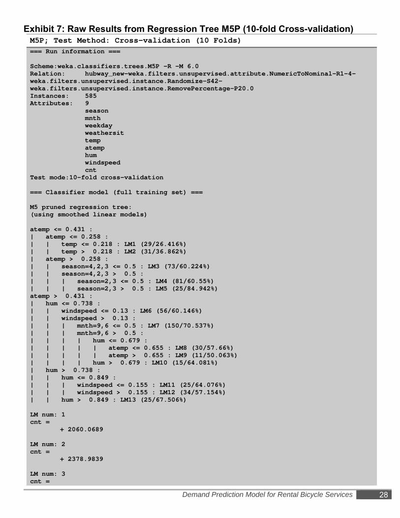
can now commence Numeric Estimation Models Tested This next subsection explains how the team derived a suitable model for estimating our output variable. A number of built-in Weka models were used and their goodness was determined by the one that has the highest correlation coefficient. Three numeric estimation models have been chosen to be tested against the training data through 10-fold Cross-validation. This technique allows us to ballpark how well the model will work with our training set and ultimately on more unseen data.

1. Linear Regression – a mathematical, linear function that predicts the output, numeric variable through a weighted sum of the input attributes Sullivan, David. “Data Mining III: Numeric Estimation”. Boston University Computer Science 105. Fall 2014. http://cs-people.bu.edu/dgs/courses/cs105/lectures/data_mining_estimation.pdf

2. Regression Tree – a decision tree model specifically designed to handle both numeric and

nominal input variables; each attribute will hold an average value for a given dataset Sullivan, David. “Data Mining III: Numeric Estimation”. Boston University Computer Science 105. Fall 2014. http://cs-people.bu.edu/dgs/courses/cs105/lectures/data_mining_estimation.pdf

3. Neural Networks – a mathematical model based on a network of links and nodes that

changes its structure based on the information that flows through the network during the learning (or training) phase Singh, Yashpal and Alok Chauhan. “Neural Networks In Data Mining”. Journal of Theoretical and Applied Information Technology. 2009. http://www.jatit.org/volumes/research-papers/Vol5No1/1Vol5No6.pdf


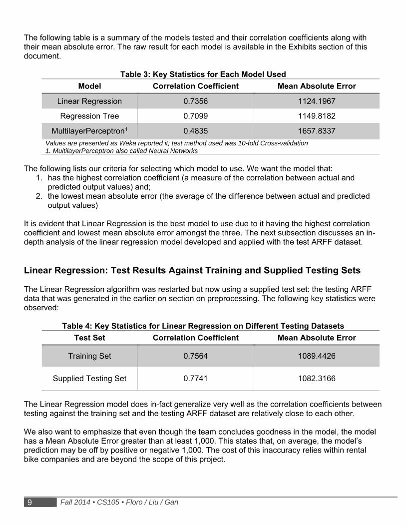
The following table is a summary of the models tested and their correlation coefficients along with their mean absolute error. The raw result for each model is available in the Exhibits section of this document.

Table 3: Key Statistics for Each Model Used

Model Correlation Coefficient Mean Absolute Error

Linear Regression 0.7356 1124.1967

Regression Tree 0.7099 1149.8182

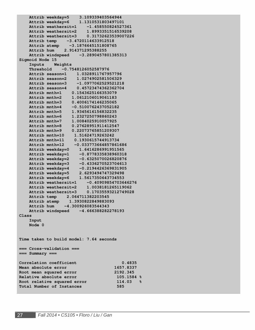
MultilayerPerceptron1 0.4835 1657.8337

Values are presented as Weka reported it; test method used was 10-fold Cross-validation 1. MultilayerPerceptron also called Neural Networks

The following lists our criteria for selecting which model to use. We want the model that:

1. has the highest correlation coefficient (a measure of the correlation between actual and predicted output values) and;

2. the lowest mean absolute error (the average of the difference between actual and predicted output values)

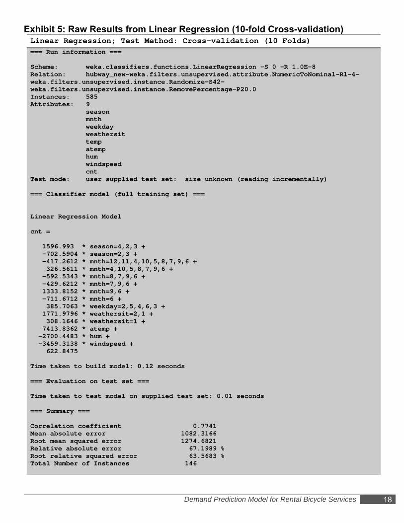
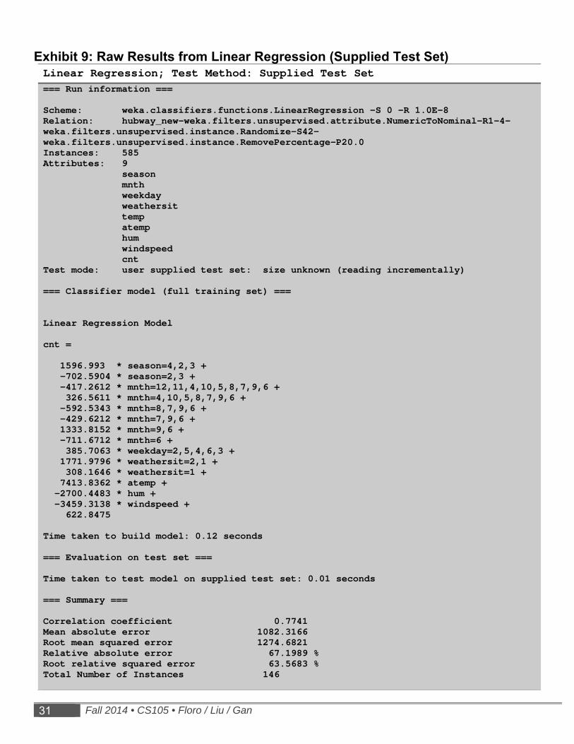
It is evident that Linear Regression is the best model to use due to it having the highest correlation coefficient and lowest mean absolute error amongst the three. The next subsection discusses an in-depth analysis of the linear regression model developed and applied with the test ARFF dataset. Linear Regression: Test Results Against Training and Supplied Testing Sets The Linear Regression algorithm was restarted but now using a supplied test set: the testing ARFF data that was generated in the earlier on section on preprocessing. The following key statistics were observed:

Table 4: Key Statistics for Linear Regression on Different Testing Datasets

Test Set Correlation Coefficient Mean Absolute Error

Training Set 0.7564 1089.4426

Supplied Testing Set 0.7741 1082.3166

The Linear Regression model does in-fact generalize very well as the correlation coefficients between testing against the training set and the testing ARFF dataset are relatively close to each other. We also want to emphasize that even though the team concludes goodness in the model, the model has a Mean Absolute Error greater than at least 1,000. This states that, on average, the model’s prediction may be off by positive or negative 1,000. The cost of this inaccuracy relies within rental bike companies and are beyond the scope of this project.


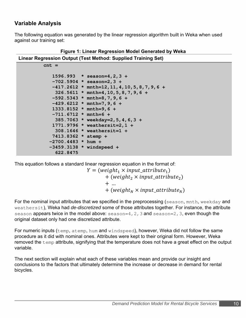
Variable Analysis The following equation was generated by the linear regression algorithm built in Weka when used against our training set:

Figure 1: Linear Regression Model Generated by Weka

Linear Regression Output (Test Method: Supplied Training Set)

cnt = 1596.993 * season=4,2,3 + -702.5904 * season=2,3 + -417.2612 * mnth=12,11,4,10,5,8,7,9,6 + 326.5611 * mnth=4,10,5,8,7,9,6 + -592.5343 * mnth=8,7,9,6 + -429.6212 * mnth=7,9,6 + 1333.8152 * mnth=9,6 + -711.6712 * mnth=6 + 385.7063 * weekday=2,5,4,6,3 + 1771.9796 * weathersit=2,1 + 308.1646 * weathersit=1 + 7413.8362 * atemp + -2700.4483 * hum + -3459.3138 * windspeed + 622.8475

This equation follows a standard linear regression equation in the format of:

_ _ … _

For the nominal input attributes that we specified in the preprocessing (season, mnth, weekday and weathersit), Weka had de-discretized some of those attributes together. For instance, the attribute season appears twice in the model above: season=4,2,3 and season=2,3, even though the original dataset only had one discretized attribute. For numeric inputs (temp, atemp, hum and windspeed), however, Weka did not follow the same procedure as it did with nominal ones. Attributes were kept to their original form. However, Weka removed the temp attribute, signifying that the temperature does not have a great effect on the output variable. The next section will explain what each of these variables mean and provide our insight and conclusions to the factors that ultimately determine the increase or decrease in demand for rental bicycles.


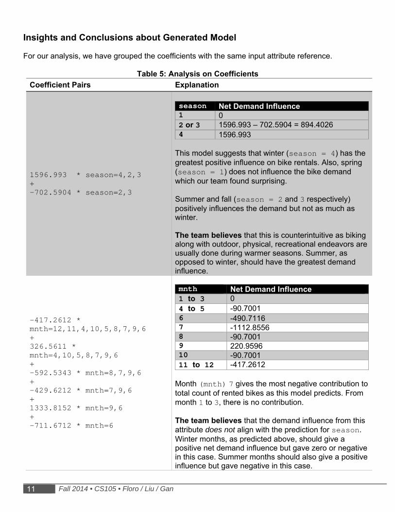
Insights and Conclusions about Generated Model For our analysis, we have grouped the coefficients with the same input attribute reference.

Table 5: Analysis on Coefficients

Coefficient Pairs Explanation

1596.993 * season=4,2,3 + -702.5904 * season=2,3

season Net Demand Influence 1 0 2 or 3 1596.993 – 702.5904 = 894.4026 4 1596.993

This model suggests that winter (season = 4) has the greatest positive influence on bike rentals. Also, spring (season = 1) does not influence the bike demand which our team found surprising. Summer and fall (season = 2 and 3 respectively) positively influences the demand but not as much as winter. The team believes that this is counterintuitive as biking along with outdoor, physical, recreational endeavors are usually done during warmer seasons. Summer, as opposed to winter, should have the greatest demand influence.

-417.2612 * mnth=12,11,4,10,5,8,7,9,6 + 326.5611 * mnth=4,10,5,8,7,9,6 + -592.5343 * mnth=8,7,9,6 + -429.6212 * mnth=7,9,6 + 1333.8152 * mnth=9,6 + -711.6712 * mnth=6

mnth Net Demand Influence 1 to 3 0 4 to 5 -90.7001 6 -490.7116 7 -1112.8556 8 -90.7001 9 220.9596 10 -90.7001 11 to 12 -417.2612

Month (mnth) 7 gives the most negative contribution to total count of rented bikes as this model predicts. From month 1 to 3, there is no contribution. The team believes that the demand influence from this attribute does not align with the prediction for season. Winter months, as predicted above, should give a positive net demand influence but gave zero or negative in this case. Summer months should also give a positive influence but gave negative in this case.


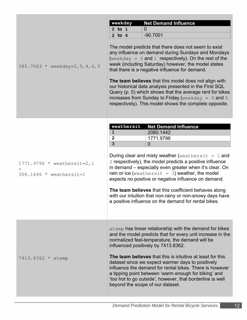
385.7063 * weekday=2,5,4,6,3

weekday Net Demand Influence 0 to 1 0 2 to 6 -90.7001

The model predicts that there does not seem to exist any influence on demand during Sundays and Mondays (weekday = 0 and 1 respectively). On the rest of the week (including Saturday) however, the model states that there is a negative influence for demand. The team believes that this model does not align with our historical data analysis presented in the First SQL Query (p. 5) which shows that the average rent for bikes increases from Sunday to Friday (weekday = 0 and 5 respectively). This model shows the complete opposite.

1771.9796 * weathersit=2,1 + 308.1646 * weathersit=1

weathersit Net Demand Influence 1 2080.1442 2 1771.9796 3 0

During clear and misty weather (weathersit = 1 and 2 respectively), the model predicts a positive influence in demand – especially even greater when it’s clear. On rain or ice (weathersit = 3) weather, the model expects no positive or negative influence on demand. The team believes that this coefficient behaves along with our intuition that non-rainy or non-snowy days have a positive influence on the demand for rental bikes.

7413.8362 * atemp

atemp has linear relationship with the demand for bikes and the model predicts that for every unit increase in the normalized feel-temperature, the demand will be influenced positively by 7413.8362. The team believes that this is intuitive at least for this dataset since we expect warmer days to positively influence the demand for rental bikes. There is however a tipping point between ‘warm enough for biking’ and ‘too hot to go outside’; however, that borderline is well beyond the scope of our dataset.


-2700.4483 * hum

hum has linear relationship with demand for bikes as the model predicts. The coefficient, -2700.4483, explains that for each unit increase in humidity, the demand for bikes will be negatively influenced by a 2700.4483 reduction in demand. As weather is more humid, less people want to rent a bike. The team believes that this is generally makes sense as higher humidity values may increase the chances of rain. The prediction for an increase in humidity leading to lower demand influence somewhat aligns with our weathersit attribute since during rain or ice the contribution will be zero.

-3459.3138 * windspeed

windspeed also has linear relationship with the demand for bikes. The negative coefficient shows that a unit increase in the wind speed, there will be a 3459.3138 negative influence for the demand. That is, as wind becomes stronger, people are less likely to get rent a bike. The team believes that this is makes sense as higher wind speeds will deter people from renting bikes.

Summary and Conclusion

In developing a model for predicting rental bike demand – our output variable, we have obtained a dataset from an external source that contains historical data on weather conditions, temperature, humidity, wind speed, month and day of the week along with our desired output variable. This dataset was divided into two files: one for 2011 and one for 2012. Before running any data mining algorithm, the raw datasets were merged so both 2011 and 2012 data were in one file and this consolidated dataset was further processed by a Python-based program that eliminates problematic attributes. The result of this was a new, single dataset without the problematic attributes. In examining the historical data, we passed the newly-generated dataset to another Python-based program that creates an SQL Relational Database. Queries were executed in this database to determine the 1.) the average rent per day of the week and; 2.) the trend of bike demand against season and weather. Visualizations were reported. Finally, the dataset was further processed in Weka to prepare it for data mining; this involves randomizing, and splitting between testing and training data. Several numeric estimation algorithms were tested against the training data, evaluating the model using 10-fold cross-validation as a ballpark examination. Linear Regression proved to be the best model to use and was tested against the training data and testing data. We conclude that the Linear Regression model developed in this analysis generalizes well with the dataset used. However, the dataset may not be ‘good enough’ to use in a real-world, business setting due a relatively low correlation coefficient.


Exhibits


Exhibit 1: First Python Program removeUnwantedRows.py # File: removeUnwantedRows.py # Authors: Yunong Louisa Gan, Jan Raphael Floro, Dan Liu # Assignment: Fall 2014 CS105 Final Project # # Description: This program takes the raw dataset CSV file, eliminates unwanted # rows (i.e. those rows that correspond to names and ids or those that will not # be useful in the data mining application). # Ask the user what the names of the input and output files are infile_name = input('Please enter the file name of the raw CSV dataset (with extensions): ') outfile_name = input('Please enter the file name of the new CSV dataset (with extensions): ') # Create file handles for both the input and output files infile = open(infile_name, mode = 'r') outfile = open(outfile_name, mode = 'w') # For each line in the input file, keep only the attributes that we want to keep for line in infile: # Split the line into a list of fields list_of_fields = line[:-1].split(',') # Initialize new list that will contain the attributes that we want to keep new_fields = ['','','','','','','','',''] # Insert those selected attributes in the new list in order new_fields[0] = list_of_fields[2] new_fields[1] = list_of_fields[4] new_fields[2] = list_of_fields[6] new_fields[3] = list_of_fields[8] new_fields[4] = list_of_fields[9] new_fields[5] = list_of_fields[10] new_fields[6] = list_of_fields[11] new_fields[7] = list_of_fields[12] new_fields[8] = list_of_fields[15] # Join new list into a string and store it in the output file new_line = ','.join(new_fields) print(new_line, file = outfile) # Close the file handles infile.close() outfile.close()


Exhibit 2: Second Python Program createTables.py # File: createTables.py # Authors: Yunong Louisa Gan, Jan Raphael Floro, Dan Liu # Assignment: Fall 2014 CS105 Final Project # # Description: This program takes the newly formatted CSV file generated by # reviewUnwantedRows.py, creates an SQLite database file and imports the # records from the CSV file to the new database file. # Import sqlite3 module import sqlite3 # Ask the user for an output file name db_filename = input('Please enter an output file name for the SQLite 3 Database (include extension, *.sqlite preferred): ') # Create the database file with the user's file name, connect to it and make a cursor db = sqlite3.connect(db_filename) cursor = db.cursor() # Create SQL table framework by creating a query and executing it agains the cursor query = ''' CREATE TABLE Hubway ( id INTEGER PRIMARY KEY, season INTEGER, month INTEGER, weekday INTEGER, weathersit INTEGER, temp REAL, feeltemp REAL, humidity REAL, windspeed REAL, rent INTEGER); ''' cursor.execute(query, []) # Open the newly created CSV file and eliminate the first line that contains the labels infile_name = input('Please enter the file name of the new CSV dataset (with extensions): ') infile = open(infile_name, mode = 'r') temporary = infile.readline() # Initialize a counter to be used as the primary key for the SQL database count = 1 # For each line in the CSV file opened, append the counter and insert the record # into the database file for line in infile: # Split line into a list of fields and insert counter into index 0 list_of_fields = line[:-1].split(',') list_of_fields.insert(0, count) # Construct an SQL query to insert values in the SQL file and execute query = ''' INSERT INTO Hubway VALUES(?, ?, ?, ?, ?, ?, ?, ?, ?, ?);''' cursor.execute(query, list_of_fields) # Add to the counter count = count + 1 #Close the file handle, commit the database and close it infile.close() db.commit() db.close()


Exhibit 3: Raw Results from First SQL Query SQL Query Result

SELECT weekday, AVG(rent) FROM Hubway GROUP BY weekday;

weekday AVG(rent) 0 4228.829 1 4338.124 2 4510.663 3 4548.538 4 4667.26 5 4690.288 6 4550.543

Exhibit 4: Raw Results from Second SQL Query

SQL Query Result

SELECT weathersit, AVG(rent) FROM Hubway WHERE season = 1 GROUP BY weathersit;

weathersit AVG(rent) 1 2811.1352 2357.1673 934.75


weathersit AVG(rent) 1 5548.5492 4236.7063 1169


weathersit AVG(rent)1 5878.2572 5222.4793 2751.75


weathersit AVG(rent)1 5043.5632 46543 1961.6


Exhibit 5: Raw Results from Linear Regression (10-fold Cross-validation) Linear Regression; Test Method: Cross-validation (10 Folds) === Run information === Scheme: weka.classifiers.functions.LinearRegression -S 0 -R 1.0E-8 Relation: hubway_new-weka.filters.unsupervised.attribute.NumericToNominal-R1-4-weka.filters.unsupervised.instance.Randomize-S42-weka.filters.unsupervised.instance.RemovePercentage-P20.0 Instances: 585 Attributes: 9 season mnth weekday weathersit temp atemp hum windspeed cnt Test mode: user supplied test set: size unknown (reading incrementally) === Classifier model (full training set) === Linear Regression Model cnt = 1596.993 * season=4,2,3 + -702.5904 * season=2,3 + -417.2612 * mnth=12,11,4,10,5,8,7,9,6 + 326.5611 * mnth=4,10,5,8,7,9,6 + -592.5343 * mnth=8,7,9,6 + -429.6212 * mnth=7,9,6 + 1333.8152 * mnth=9,6 + -711.6712 * mnth=6 + 385.7063 * weekday=2,5,4,6,3 + 1771.9796 * weathersit=2,1 + 308.1646 * weathersit=1 + 7413.8362 * atemp + -2700.4483 * hum + -3459.3138 * windspeed + 622.8475 Time taken to build model: 0.12 seconds === Evaluation on test set === Time taken to test model on supplied test set: 0.01 seconds === Summary === Correlation coefficient 0.7741 Mean absolute error 1082.3166 Root mean squared error 1274.6821 Relative absolute error 67.1989 % Root relative squared error 63.5683 % Total Number of Instances 146


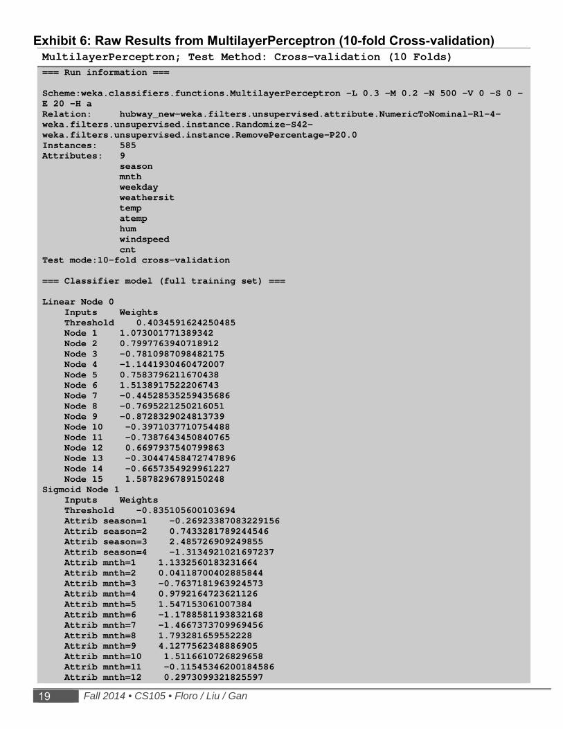
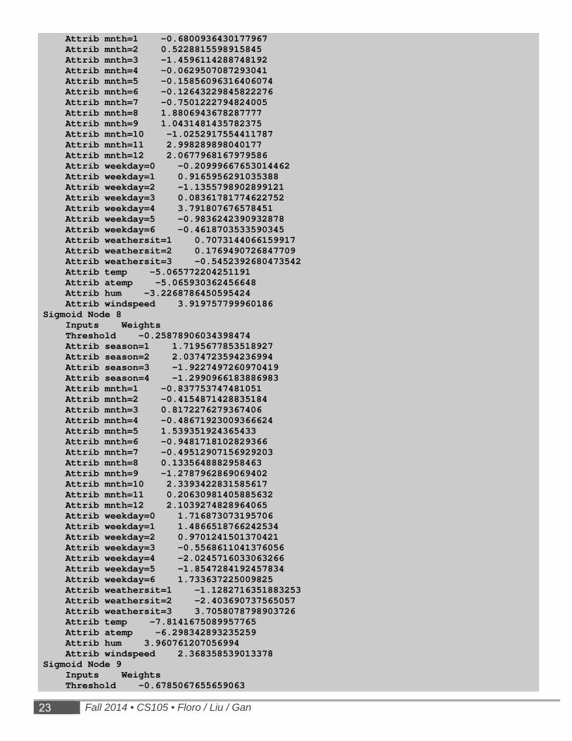
Exhibit 6: Raw Results from MultilayerPerceptron (10-fold Cross-validation) MultilayerPerceptron; Test Method: Cross-validation (10 Folds) === Run information === Scheme:weka.classifiers.functions.MultilayerPerceptron -L 0.3 -M 0.2 -N 500 -V 0 -S 0 -E 20 -H a Relation: hubway_new-weka.filters.unsupervised.attribute.NumericToNominal-R1-4-weka.filters.unsupervised.instance.Randomize-S42-weka.filters.unsupervised.instance.RemovePercentage-P20.0 Instances: 585 Attributes: 9 season mnth weekday weathersit temp atemp hum windspeed cnt Test mode:10-fold cross-validation === Classifier model (full training set) === Linear Node 0 Inputs Weights Threshold 0.4034591624250485 Node 1 1.073001771389342 Node 2 0.7997763940718912 Node 3 -0.7810987098482175 Node 4 -1.1441930460472007 Node 5 0.7583796211670438 Node 6 1.5138917522206743 Node 7 -0.44528535259435686 Node 8 -0.7695221250216051 Node 9 -0.8728329024813739 Node 10 -0.3971037710754488 Node 11 -0.7387643450840765 Node 12 0.6697937540799863 Node 13 -0.30447458472747896 Node 14 -0.6657354929961227 Node 15 1.5878296789150248 Sigmoid Node 1 Inputs Weights Threshold -0.835105600103694 Attrib season=1 -0.26923387083229156 Attrib season=2 0.7433281789244546 Attrib season=3 2.485726909249855 Attrib season=4 -1.3134921021697237 Attrib mnth=1 1.1332560183231664 Attrib mnth=2 0.04118700402885844 Attrib mnth=3 -0.7637181963924573 Attrib mnth=4 0.9792164723621126 Attrib mnth=5 1.547153061007384 Attrib mnth=6 -1.1788581193832168 Attrib mnth=7 -1.4667373709969456 Attrib mnth=8 1.793281659552228 Attrib mnth=9 4.1277562348886905 Attrib mnth=10 1.5116610726829658 Attrib mnth=11 -0.11545346200184586 Attrib mnth=12 0.2973099321825597


Attrib weekday=0 0.0735713150735382 Attrib weekday=1 -0.13531496279818347 Attrib weekday=2 0.18891798030488438 Attrib weekday=3 -0.15302105370984156 Attrib weekday=4 0.756820806490527 Attrib weekday=5 3.2669990717655377 Attrib weekday=6 -0.013196966833346382 Attrib weathersit=1 1.8987162613074986 Attrib weathersit=2 -0.9220489355100241 Attrib weathersit=3 -0.16574050012262911 Attrib temp -0.3462691238736456 Attrib atemp -0.7232156351891944 Attrib hum -7.555827566193684 Attrib windspeed 1.2149137740743714 Sigmoid Node 2 Inputs Weights Threshold -0.6272845810275781 Attrib season=1 0.4511309813560522 Attrib season=2 0.3243673306399936 Attrib season=3 -0.14462217443822908 Attrib season=4 0.5717810187426616 Attrib mnth=1 -1.0620271502105918 Attrib mnth=2 1.5029576238066138 Attrib mnth=3 0.7370720015247065 Attrib mnth=4 -1.4484679734569135 Attrib mnth=5 1.2193167796387365 Attrib mnth=6 2.232955502400696 Attrib mnth=7 0.06715219650782216 Attrib mnth=8 0.38798295516628284 Attrib mnth=9 0.29551875297827473 Attrib mnth=10 1.3849939708300956 Attrib mnth=11 0.9129130515295194 Attrib mnth=12 -0.14512949985777754 Attrib weekday=0 1.9931321860448894 Attrib weekday=1 3.1967624812276476 Attrib weekday=2 -1.0879978182772783 Attrib weekday=3 0.457659508255081 Attrib weekday=4 1.4975764986214952 Attrib weekday=5 -0.9953808172895143 Attrib weekday=6 -2.075406651189462 Attrib weathersit=1 1.6415054200085994 Attrib weathersit=2 0.010771694877575056 Attrib weathersit=3 -1.145614687211436 Attrib temp 0.3062507318500584 Attrib atemp 1.4272500834524942 Attrib hum -3.7023979230445248 Attrib windspeed 3.43243162409721 Sigmoid Node 3 Inputs Weights Threshold -1.099251439861587 Attrib season=1 -0.2983352128311242 Attrib season=2 1.2266648481842768 Attrib season=3 1.3776057739283585 Attrib season=4 -0.16892801822017262 Attrib mnth=1 0.32915348891007523 Attrib mnth=2 3.2794585387928885 Attrib mnth=3 0.5737609948893269 Attrib mnth=4 0.945881493134643 Attrib mnth=5 -1.0281547724703388 Attrib mnth=6 -0.20111870519034677 Attrib mnth=7 2.426206310650778 Attrib mnth=8 1.3134003894101203


Attrib mnth=9 0.8637602321512693 Attrib mnth=10 3.7722260235020193 Attrib mnth=11 -1.7180240810799472 Attrib mnth=12 0.34500229426844337 Attrib weekday=0 -1.2359496617461008 Attrib weekday=1 -1.2523303956510252 Attrib weekday=2 -0.0512640219334471 Attrib weekday=3 5.0344463244969555 Attrib weekday=4 3.1705493865198813 Attrib weekday=5 -0.7969667993073348 Attrib weekday=6 0.5012732532805586 Attrib weathersit=1 -1.3808865602742402 Attrib weathersit=2 3.687279205414965 Attrib weathersit=3 -1.263950856900867 Attrib temp -1.6025642890452991 Attrib atemp -1.2460303406397897 Attrib hum 3.806611025524226 Attrib windspeed 2.1413694085068093 Sigmoid Node 4 Inputs Weights Threshold -0.6125614054374625 Attrib season=1 2.301339192069271 Attrib season=2 0.21595465624979585 Attrib season=3 -2.002381472625347 Attrib season=4 0.5776248990007989 Attrib mnth=1 1.4147139027031674 Attrib mnth=2 -0.7873093719742582 Attrib mnth=3 -1.4647000862547463 Attrib mnth=4 0.30894778422015495 Attrib mnth=5 0.11744997371496953 Attrib mnth=6 1.678371884010929 Attrib mnth=7 0.2601669996084536 Attrib mnth=8 0.7165572253867979 Attrib mnth=9 -0.9759034972248922 Attrib mnth=10 -1.2035074076468777 Attrib mnth=11 3.881580115131238 Attrib mnth=12 1.6673594234003442 Attrib weekday=0 2.430737585641643 Attrib weekday=1 -0.029305707349405366 Attrib weekday=2 -0.2809770028027914 Attrib weekday=3 -1.002602704706082 Attrib weekday=4 0.29385881269950076 Attrib weekday=5 -0.4171895892417452 Attrib weekday=6 1.831364169728795 Attrib weathersit=1 -1.702663907847466 Attrib weathersit=2 0.8307789973732239 Attrib weathersit=3 1.4086185714457284 Attrib temp 4.765107492570161 Attrib atemp 5.397309969510869 Attrib hum 2.6743033792236504 Attrib windspeed 4.843385409840476 Sigmoid Node 5 Inputs Weights Threshold -0.7702271035603074 Attrib season=1 -0.7912698399661623 Attrib season=2 1.3342816535525144 Attrib season=3 -2.06004550322802 Attrib season=4 3.0002838609962175 Attrib mnth=1 0.6274233404933738 Attrib mnth=2 0.004961995450475025 Attrib mnth=3 2.1208962407896137 Attrib mnth=4 -1.5587774103063154


Attrib mnth=5 0.7756856754052758 Attrib mnth=6 1.6368281383100256 Attrib mnth=7 -0.3001713973913252 Attrib mnth=8 0.8685151927718178 Attrib mnth=9 3.178730593716785 Attrib mnth=10 2.1142799632718488 Attrib mnth=11 0.3236981666904239 Attrib mnth=12 -2.336499036978622 Attrib weekday=0 -0.5993469100502076 Attrib weekday=1 -0.650182502557702 Attrib weekday=2 1.899648613421824 Attrib weekday=3 1.511829159936197 Attrib weekday=4 0.8699142634040725 Attrib weekday=5 -0.9403406416835125 Attrib weekday=6 1.6589672748963804 Attrib weathersit=1 -0.41529560006794974 Attrib weathersit=2 2.5393108952031054 Attrib weathersit=3 -1.3495279722872315 Attrib temp 1.6766375355576937 Attrib atemp 1.3960864802250765 Attrib hum -8.51696696650129 Attrib windspeed -3.7266593200778106 Sigmoid Node 6 Inputs Weights Threshold -0.9771847570286205 Attrib season=1 -0.2613288541630906 Attrib season=2 1.8662783168120032 Attrib season=3 -0.005021092531550224 Attrib season=4 0.20377775514061652 Attrib mnth=1 0.7870300635035192 Attrib mnth=2 0.6277338920383292 Attrib mnth=3 2.661395650848618 Attrib mnth=4 2.515850786190174 Attrib mnth=5 -0.7248311343538938 Attrib mnth=6 -1.0813811680170495 Attrib mnth=7 -1.3427485472166332 Attrib mnth=8 2.372020219049747 Attrib mnth=9 0.7357792316702811 Attrib mnth=10 2.341063329857603 Attrib mnth=11 0.19807007779987235 Attrib mnth=12 0.5071342076845808 Attrib weekday=0 -0.3763085296193364 Attrib weekday=1 -0.22802440531751533 Attrib weekday=2 1.5205637874092304 Attrib weekday=3 0.6334056582596763 Attrib weekday=4 0.43738828897372356 Attrib weekday=5 2.9876502082369476 Attrib weekday=6 -0.1924315838130855 Attrib weathersit=1 -0.018308474406878796 Attrib weathersit=2 1.1611455705184723 Attrib weathersit=3 -0.13424346857657693 Attrib temp 3.1192446832459173 Attrib atemp 3.475714046525946 Attrib hum 1.5964812593854052 Attrib windspeed -5.884628344985574 Sigmoid Node 7 Inputs Weights Threshold -0.4529682814682877 Attrib season=1 1.5791493238974204 Attrib season=2 -0.7650458514198675 Attrib season=3 1.1605783776784193 Attrib season=4 -1.1050749606551218


Attrib mnth=1 -0.6800936430177967 Attrib mnth=2 0.5228815598915845 Attrib mnth=3 -1.4596114288748192 Attrib mnth=4 -0.0629507087293041 Attrib mnth=5 -0.15856096316406074 Attrib mnth=6 -0.12643229845822276 Attrib mnth=7 -0.7501222794824005 Attrib mnth=8 1.8806943678287777 Attrib mnth=9 1.0431481435782375 Attrib mnth=10 -1.0252917554411787 Attrib mnth=11 2.998289898040177 Attrib mnth=12 2.0677968167979586 Attrib weekday=0 -0.20999667653014462 Attrib weekday=1 0.9165956291035388 Attrib weekday=2 -1.1355798902899121 Attrib weekday=3 0.08361781774622752 Attrib weekday=4 3.791807676578451 Attrib weekday=5 -0.9836242390932878 Attrib weekday=6 -0.4618703533590345 Attrib weathersit=1 0.7073144066159917 Attrib weathersit=2 0.1769490726847709 Attrib weathersit=3 -0.5452392680473542 Attrib temp -5.065772204251191 Attrib atemp -5.065930362456648 Attrib hum -3.2268786450595424 Attrib windspeed 3.919757799960186 Sigmoid Node 8 Inputs Weights Threshold -0.25878906034398474 Attrib season=1 1.7195677853518927 Attrib season=2 2.0374723594236994 Attrib season=3 -1.9227497260970419 Attrib season=4 -1.2990966183886983 Attrib mnth=1 -0.837753747481051 Attrib mnth=2 -0.4154871428835184 Attrib mnth=3 0.8172276279367406 Attrib mnth=4 -0.48671923009366624 Attrib mnth=5 1.539351924365433 Attrib mnth=6 -0.9481718102829366 Attrib mnth=7 -0.49512907156929203 Attrib mnth=8 0.1335648882958463 Attrib mnth=9 -1.2787962869069402 Attrib mnth=10 2.3393422831585617 Attrib mnth=11 0.20630981405885632 Attrib mnth=12 2.1039274828964065 Attrib weekday=0 1.716873073195706 Attrib weekday=1 1.4866518766242534 Attrib weekday=2 0.9701241501370421 Attrib weekday=3 -0.5568611041376056 Attrib weekday=4 -2.0245716033063266 Attrib weekday=5 -1.8547284192457834 Attrib weekday=6 1.733637225009825 Attrib weathersit=1 -1.1282716351883253 Attrib weathersit=2 -2.403690737565057 Attrib weathersit=3 3.7058078798903726 Attrib temp -7.8141675089957765 Attrib atemp -6.298342893235259 Attrib hum 3.960761207056994 Attrib windspeed 2.368358539013378 Sigmoid Node 9 Inputs Weights Threshold -0.6785067655659063


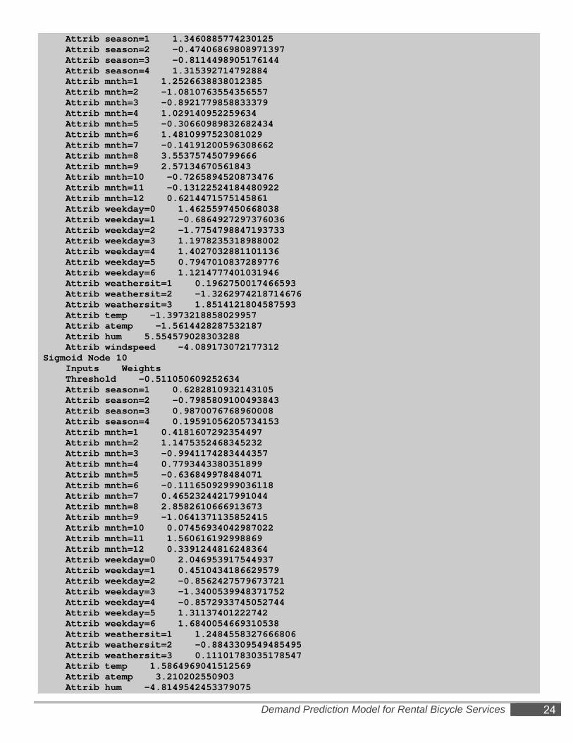
Attrib season=1 1.3460885774230125 Attrib season=2 -0.47406869808971397 Attrib season=3 -0.8114498905176144 Attrib season=4 1.315392714792884 Attrib mnth=1 1.2526638838012385 Attrib mnth=2 -1.0810763554356557 Attrib mnth=3 -0.8921779858833379 Attrib mnth=4 1.029140952259634 Attrib mnth=5 -0.30660989832682434 Attrib mnth=6 1.4810997523081029 Attrib mnth=7 -0.14191200596308662 Attrib mnth=8 3.553757450799666 Attrib mnth=9 2.57134670561843 Attrib mnth=10 -0.7265894520873476 Attrib mnth=11 -0.13122524184480922 Attrib mnth=12 0.6214471575145861 Attrib weekday=0 1.4625597450668038 Attrib weekday=1 -0.6864927297376036 Attrib weekday=2 -1.7754798847193733 Attrib weekday=3 1.1978235318988002 Attrib weekday=4 1.4027032881101136 Attrib weekday=5 0.7947010837289776 Attrib weekday=6 1.1214777401031946 Attrib weathersit=1 0.1962750017466593 Attrib weathersit=2 -1.3262974218714676 Attrib weathersit=3 1.8514121804587593 Attrib temp -1.3973218858029957 Attrib atemp -1.5614428287532187 Attrib hum 5.554579028303288 Attrib windspeed -4.089173072177312 Sigmoid Node 10 Inputs Weights Threshold -0.511050609252634 Attrib season=1 0.6282810932143105 Attrib season=2 -0.7985809100493843 Attrib season=3 0.9870076768960008 Attrib season=4 0.19591056205734153 Attrib mnth=1 0.4181607292354497 Attrib mnth=2 1.1475352468345232 Attrib mnth=3 -0.9941174283444357 Attrib mnth=4 0.7793443380351899 Attrib mnth=5 -0.636849978484071 Attrib mnth=6 -0.11165092999036118 Attrib mnth=7 0.46523244217991044 Attrib mnth=8 2.8582610666913673 Attrib mnth=9 -1.0641371135852415 Attrib mnth=10 0.07456934042987022 Attrib mnth=11 1.560616192998869 Attrib mnth=12 0.3391244816248364 Attrib weekday=0 2.046953917544937 Attrib weekday=1 0.4510434186629579 Attrib weekday=2 -0.8562427579673721 Attrib weekday=3 -1.3400539948371752 Attrib weekday=4 -0.8572933745052744 Attrib weekday=5 1.31137401222742 Attrib weekday=6 1.6840054669310538 Attrib weathersit=1 1.2484558327666806 Attrib weathersit=2 -0.8843309549485495 Attrib weathersit=3 0.11101783035178547 Attrib temp 1.5864969041512569 Attrib atemp 3.210202550903 Attrib hum -4.8149542453379075


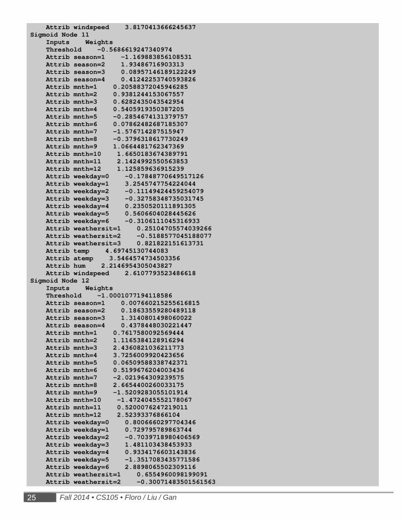
Attrib windspeed 3.8170413666245637Sigmoid Node 11 Inputs Weights Threshold -0.5686619247340974 Attrib season=1 -1.169883856108531 Attrib season=2 1.93486716903313 Attrib season=3 0.08957146189122249 Attrib season=4 0.41242253740593826 Attrib mnth=1 0.20588372045946285 Attrib mnth=2 0.9381244153067557 Attrib mnth=3 0.6282435043542954 Attrib mnth=4 0.5405919350387205 Attrib mnth=5 -0.2854674131379757 Attrib mnth=6 0.07862482687185307 Attrib mnth=7 -1.576714287515947 Attrib mnth=8 -0.3796318617730249 Attrib mnth=9 1.0664481762347369 Attrib mnth=10 1.6650183674389791 Attrib mnth=11 2.1424992550563853 Attrib mnth=12 1.125859636915239 Attrib weekday=0 -0.17848770649517126 Attrib weekday=1 3.2545747754224044 Attrib weekday=2 -0.11149424459254079 Attrib weekday=3 -0.32758348735031745 Attrib weekday=4 0.2350520111891305 Attrib weekday=5 0.5606604028445626 Attrib weekday=6 -0.3106111045316933 Attrib weathersit=1 0.25104705574039266 Attrib weathersit=2 -0.5188577045188077 Attrib weathersit=3 0.821822151613731 Attrib temp 4.69745130744083 Attrib atemp 3.5464574734503356 Attrib hum 2.2146954305043827 Attrib windspeed 2.6107793523486618 Sigmoid Node 12 Inputs Weights Threshold -1.0001077194118586 Attrib season=1 0.007660215255616815 Attrib season=2 0.18633559280489118 Attrib season=3 1.3140801498060022 Attrib season=4 0.4378448030221447 Attrib mnth=1 0.7617580092569444 Attrib mnth=2 1.1165384128916294 Attrib mnth=3 2.4360821036211773 Attrib mnth=4 3.7256009920423656 Attrib mnth=5 0.06509588338742371 Attrib mnth=6 0.5199676204003436 Attrib mnth=7 -2.021964309239575 Attrib mnth=8 2.6654400260033175 Attrib mnth=9 -1.5209283055101914 Attrib mnth=10 -1.4724045552178067 Attrib mnth=11 0.5200076247219011 Attrib mnth=12 2.52393376866104 Attrib weekday=0 0.8006660297704346 Attrib weekday=1 0.729795789863744 Attrib weekday=2 -0.7039718980406569 Attrib weekday=3 1.481103438453933 Attrib weekday=4 0.9334176603143836 Attrib weekday=5 -1.3517083435771586 Attrib weekday=6 2.8898065502309116 Attrib weathersit=1 0.6554960098199091 Attrib weathersit=2 -0.30071483501561563


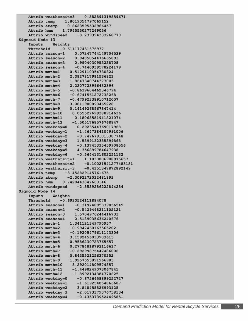
Attrib weathersit=3 0.582891319859671 Attrib temp 1.8019054797069152 Attrib atemp 0.8623595532966457 Attrib hum 1.7945550277269056 Attrib windspeed -8.239394333260778 Sigmoid Node 13 Inputs Weights Threshold -0.611177431376937 Attrib season=1 0.07247744149706539 Attrib season=2 0.9485054476665893 Attrib season=3 0.9904030953238708 Attrib season=4 -0.7440939578224179 Attrib mnth=1 0.5129110354730324 Attrib mnth=2 2.3827817981536823 Attrib mnth=3 1.8647340744377003 Attrib mnth=4 2.2207723996432396 Attrib mnth=5 -0.8639604462346794 Attrib mnth=6 -0.6741561272738268 Attrib mnth=7 -0.47992338910712007 Attrib mnth=8 3.0811980898465228 Attrib mnth=9 0.14149268967847414 Attrib mnth=10 0.055527699388914636 Attrib mnth=11 -0.18068581941821074 Attrib mnth=12 -1.5051768576768847 Attrib weekday=0 0.2923544769017968 Attrib weekday=1 -1.4647384104991006 Attrib weekday=2 -0.7476791015307748 Attrib weekday=3 1.5899132385399868 Attrib weekday=4 -0.13745335459908556 Attrib weekday=5 4.356899784647938 Attrib weekday=6 -0.5644131602251132 Attrib weathersit=1 1.1830806908975657 Attrib weathersit=2 -0.10021541277483181 Attrib weathersit=3 -0.4151347872892149 Attrib temp -3.452829145761675 Attrib atemp -2.3092272032481893 Attrib hum 0.7428443847660146 Attrib windspeed -2.5539286222844284 Sigmoid Node 14 Inputs Weights Threshold -0.6930524111884078 Attrib season=1 -0.31974095339856545 Attrib season=2 -0.5429448211105121 Attrib season=3 1.5704976244416733 Attrib season=4 0.5189035636240676 Attrib mnth=1 1.341121349790957 Attrib mnth=2 -0.9942460163565202 Attrib mnth=3 -0.19205479611143306 Attrib mnth=4 3.1592456033903615 Attrib mnth=5 0.9586230723765657 Attrib mnth=6 0.27784818793116617 Attrib mnth=7 -0.29299875442486006 Attrib mnth=8 0.8435521256370252 Attrib mnth=9 1.9257553891966983 Attrib mnth=10 3.292014809574857 Attrib mnth=11 -1.4498249073067841 Attrib mnth=12 -1.8992134384770225 Attrib weekday=0 -0.6756458899252727 Attrib weekday=1 -1.619254054866607 Attrib weekday=2 3.848458826993125 Attrib weekday=3 -2.0173379376758134 Attrib weekday=4 -0.4353739524495851


Attrib weekday=5 3.109339403564944 Attrib weekday=6 1.1310531803497101 Attrib weathersit=1 -1.458550824527361 Attrib weathersit=2 1.8993351516539208 Attrib weathersit=3 0.31732623539007226 Attrib temp -3.4720114633912518 Attrib atemp -3.1876645151808765 Attrib hum 2.914371295388255 Attrib windspeed -3.2890457801385313 Sigmoid Node 15 Inputs Weights Threshold -0.7548126052587976 Attrib season=1 1.0328911767957796 Attrib season=2 1.0274902581506329 Attrib season=3 -1.0977062529521218 Attrib season=4 0.45723474362362704 Attrib mnth=1 0.1543625166353079 Attrib mnth=2 1.0612106019061183 Attrib mnth=3 0.4006174146235065 Attrib mnth=4 -0.5100762437052182 Attrib mnth=5 1.9345616156832235 Attrib mnth=6 1.2327250798860243 Attrib mnth=7 1.0084025910057925 Attrib mnth=8 0.27628951911412547 Attrib mnth=9 0.22073765851209307 Attrib mnth=10 1.51624719263242 Attrib mnth=11 0.1930615744913734 Attrib mnth=12 -0.033773664857861686 Attrib weekday=0 1.6416286991951565 Attrib weekday=1 -0.8778335838960318 Attrib weekday=2 -0.6325070026820876 Attrib weekday=3 -0.4336270523704613 Attrib weekday=4 -0.2194426369831905 Attrib weekday=5 2.6293494747329498 Attrib weekday=6 1.5617350643734553 Attrib weathersit=1 -0.40909854703646276 Attrib weathersit=2 1.0038181265119062 Attrib weathersit=3 0.17035593212749028 Attrib temp 2.064711382203545 Attrib atemp 1.3930822849883093 Attrib hum -4.300926083544343 Attrib windspeed -4.666388282278193 Class Input Node 0 Time taken to build model: 7.64 seconds === Cross-validation === === Summary === Correlation coefficient 0.4835 Mean absolute error 1657.8337 Root mean squared error 2192.345 Relative absolute error 105.1584 % Root relative squared error 114.03 % Total Number of Instances 585


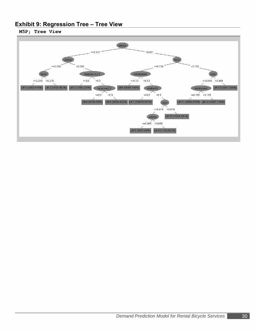
Exhibit 7: Raw Results from Regression Tree M5P (10-fold Cross-validation) M5P; Test Method: Cross-validation (10 Folds) === Run information === Scheme:weka.classifiers.trees.M5P -R -M 6.0 Relation: hubway_new-weka.filters.unsupervised.attribute.NumericToNominal-R1-4-weka.filters.unsupervised.instance.Randomize-S42-weka.filters.unsupervised.instance.RemovePercentage-P20.0 Instances: 585 Attributes: 9 season mnth weekday weathersit temp atemp hum windspeed cnt Test mode:10-fold cross-validation === Classifier model (full training set) === M5 pruned regression tree: (using smoothed linear models) atemp <= 0.431 : | atemp <= 0.258 : | | temp <= 0.218 : LM1 (29/26.416%) | | temp > 0.218 : LM2 (31/36.862%) | atemp > 0.258 : | | season=4,2,3 <= 0.5 : LM3 (73/60.224%) | | season=4,2,3 > 0.5 : | | | season=2,3 <= 0.5 : LM4 (81/60.55%) | | | season=2,3 > 0.5 : LM5 (25/84.942%) atemp > 0.431 : | hum <= 0.738 : | | windspeed <= 0.13 : LM6 (56/60.146%) | | windspeed > 0.13 : | | | mnth=9,6 <= 0.5 : LM7 (150/70.537%) | | | mnth=9,6 > 0.5 : | | | | hum <= 0.679 : | | | | | atemp <= 0.655 : LM8 (30/57.66%) | | | | | atemp > 0.655 : LM9 (11/50.063%) | | | | hum > 0.679 : LM10 (15/64.081%) | hum > 0.738 : | | hum <= 0.849 : | | | windspeed <= 0.155 : LM11 (25/64.076%) | | | windspeed > 0.155 : LM12 (34/57.154%) | | hum > 0.849 : LM13 (25/67.506%) LM num: 1 cnt = + 2060.0689 LM num: 2 cnt = + 2378.9839 LM num: 3 cnt =


+ 3154.0922 LM num: 4 cnt = + 4242.4465 LM num: 5 cnt = + 3653.44 LM num: 6 cnt = + 6198.3408 LM num: 7 cnt = + 5488.4579 LM num: 8 cnt = + 6382.4125 LM num: 9 cnt = + 5990.584 LM num: 10 cnt = + 5684.426 LM num: 11 cnt = + 5408.337 LM num: 12 cnt = + 4785.3039 LM num: 13 cnt = + 4108.4235 Number of Rules : 13 Time taken to build model: 0.5 seconds === Cross-validation === === Summary === Correlation coefficient 0.7099 Mean absolute error 1149.8182 Root mean squared error 1357.5547 Relative absolute error 72.9343 % Root relative squared error 70.6102 % Total Number of Instances 585


Exhibit 9: Regression Tree – Tree View M5P; Tree View


Exhibit 9: Raw Results from Linear Regression (Supplied Test Set) Linear Regression; Test Method: Supplied Test Set === Run information === Scheme: weka.classifiers.functions.LinearRegression -S 0 -R 1.0E-8 Relation: hubway_new-weka.filters.unsupervised.attribute.NumericToNominal-R1-4-weka.filters.unsupervised.instance.Randomize-S42-weka.filters.unsupervised.instance.RemovePercentage-P20.0 Instances: 585 Attributes: 9 season mnth weekday weathersit temp atemp hum windspeed cnt Test mode: user supplied test set: size unknown (reading incrementally) === Classifier model (full training set) === Linear Regression Model cnt = 1596.993 * season=4,2,3 + -702.5904 * season=2,3 + -417.2612 * mnth=12,11,4,10,5,8,7,9,6 + 326.5611 * mnth=4,10,5,8,7,9,6 + -592.5343 * mnth=8,7,9,6 + -429.6212 * mnth=7,9,6 + 1333.8152 * mnth=9,6 + -711.6712 * mnth=6 + 385.7063 * weekday=2,5,4,6,3 + 1771.9796 * weathersit=2,1 + 308.1646 * weathersit=1 + 7413.8362 * atemp + -2700.4483 * hum + -3459.3138 * windspeed + 622.8475 Time taken to build model: 0.12 seconds === Evaluation on test set === Time taken to test model on supplied test set: 0.01 seconds === Summary === Correlation coefficient 0.7741 Mean absolute error 1082.3166 Root mean squared error 1274.6821 Relative absolute error 67.1989 % Root relative squared error 63.5683 % Total Number of Instances 146

CS105 - Final Project

Documents

Transcript of CS105 - Final Project