CS 445 / 645 Introduction to Computer Graphics Lecture 23 Bézier Curves Lecture 23 Bézier Curves.
33
CS 445 / 645 Introduction to Computer Graphics Lecture 23 Lecture 23 B B ézier Curves ézier Curves
-
Upload
luke-harrell -
Category
Documents
-
view
229 -
download
4
Transcript of CS 445 / 645 Introduction to Computer Graphics Lecture 23 Bézier Curves Lecture 23 Bézier Curves.
CS 445 / 645Introduction to Computer Graphics
Lecture 23Lecture 23
BBézier Curvesézier Curves
Lecture 23Lecture 23
BBézier Curvesézier Curves
Splines - History
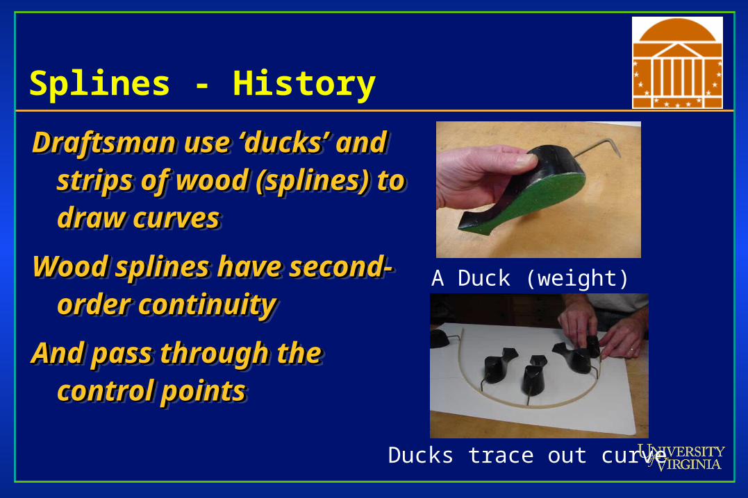
Draftsman use ‘ducks’ and Draftsman use ‘ducks’ and strips of wood (splines) to strips of wood (splines) to draw curvesdraw curves
Wood splines have second-Wood splines have second-order continuityorder continuity
And pass through the And pass through the control pointscontrol points
Draftsman use ‘ducks’ and Draftsman use ‘ducks’ and strips of wood (splines) to strips of wood (splines) to draw curvesdraw curves
Wood splines have second-Wood splines have second-order continuityorder continuity
And pass through the And pass through the control pointscontrol points
A Duck (weight)
Ducks trace out curve
Bézier Curves
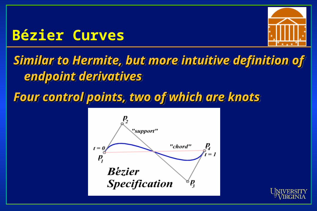
Similar to Hermite, but more intuitive definition of Similar to Hermite, but more intuitive definition of endpoint derivativesendpoint derivatives
Four control points, two of which are knotsFour control points, two of which are knots
Similar to Hermite, but more intuitive definition of Similar to Hermite, but more intuitive definition of endpoint derivativesendpoint derivatives
Four control points, two of which are knotsFour control points, two of which are knots
Bézier Curves
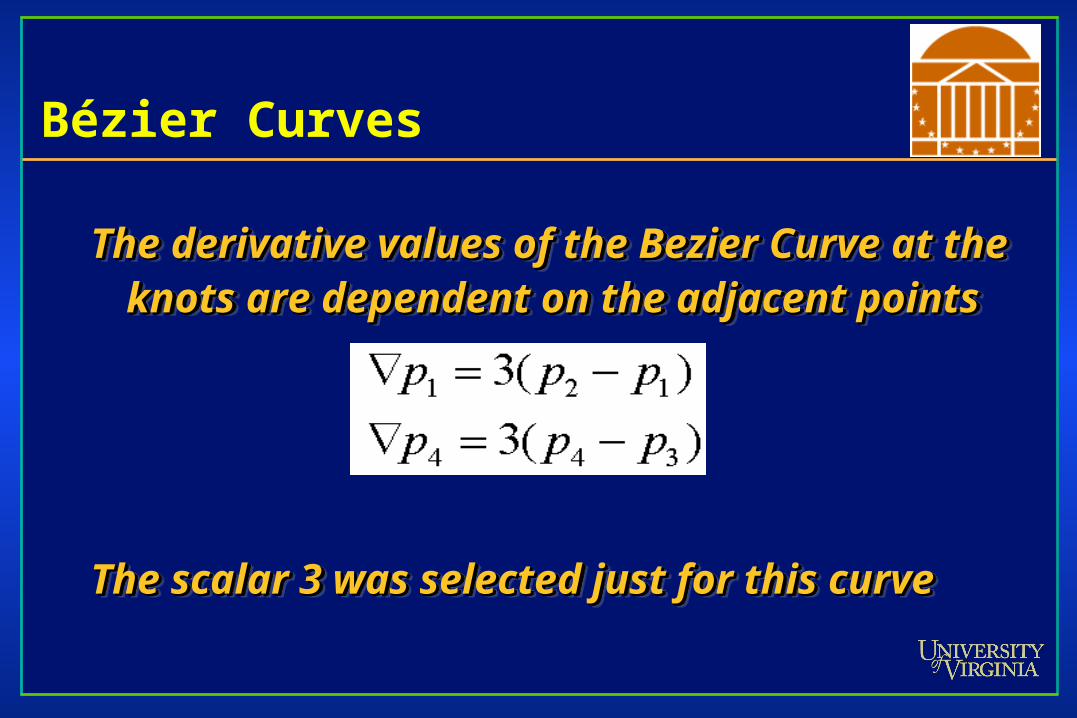
The derivative values of the Bezier Curve at the The derivative values of the Bezier Curve at the knots are dependent on the adjacent pointsknots are dependent on the adjacent points
The scalar 3 was selected just for this curve The scalar 3 was selected just for this curve
The derivative values of the Bezier Curve at the The derivative values of the Bezier Curve at the knots are dependent on the adjacent pointsknots are dependent on the adjacent points
The scalar 3 was selected just for this curve The scalar 3 was selected just for this curve
Bézier vs. Hermite
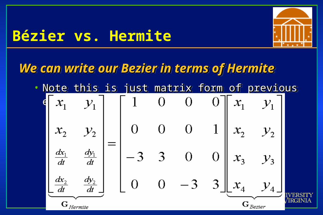
We can write our Bezier in terms of HermiteWe can write our Bezier in terms of Hermite
• Note this is just matrix form of previous equationsNote this is just matrix form of previous equations
We can write our Bezier in terms of HermiteWe can write our Bezier in terms of Hermite
• Note this is just matrix form of previous equationsNote this is just matrix form of previous equations
Bézier vs. Hermite
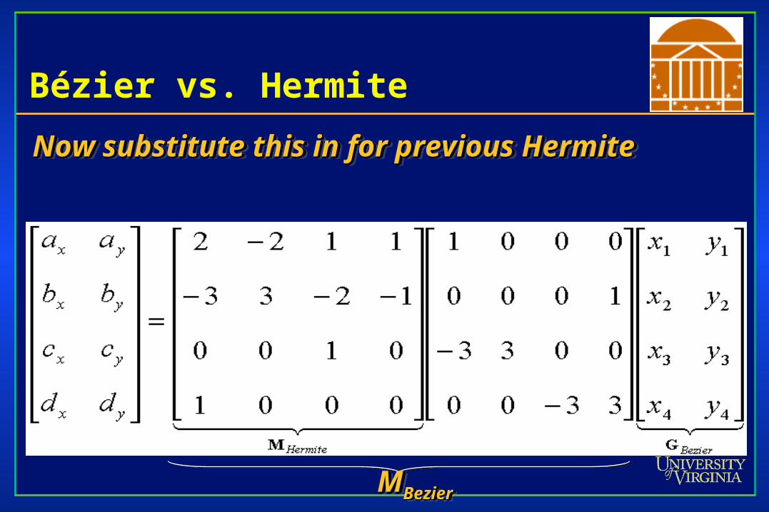
Now substitute this in for previous HermiteNow substitute this in for previous HermiteNow substitute this in for previous HermiteNow substitute this in for previous Hermite
MMBezierBezierMMBezierBezier
Bézier Basis and Geometry Matrices
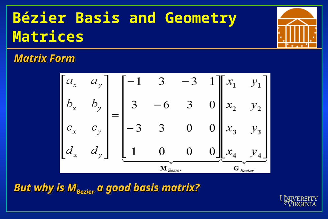
Matrix FormMatrix Form
But why is MBut why is MBezierBezier a good basis matrix? a good basis matrix?
Matrix FormMatrix Form
But why is MBut why is MBezierBezier a good basis matrix? a good basis matrix?
Bézier Blending Functions
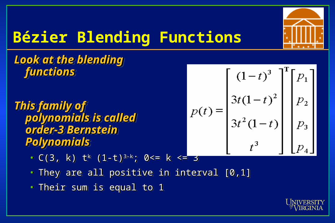
Look at the blending Look at the blending functionsfunctions
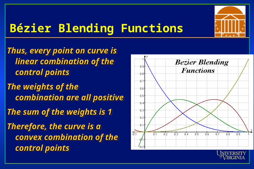
This family of This family of polynomials is calledpolynomials is calledorder-3 Bernstein order-3 Bernstein PolynomialsPolynomials• C(3, k) tC(3, k) tkk (1-t) (1-t)3-k3-k; 0<= k <= 3; 0<= k <= 3
• They are all positive in interval [0,1]They are all positive in interval [0,1]
• Their sum is equal to 1Their sum is equal to 1
Look at the blending Look at the blending functionsfunctions
This family of This family of polynomials is calledpolynomials is calledorder-3 Bernstein order-3 Bernstein PolynomialsPolynomials• C(3, k) tC(3, k) tkk (1-t) (1-t)3-k3-k; 0<= k <= 3; 0<= k <= 3
• They are all positive in interval [0,1]They are all positive in interval [0,1]
• Their sum is equal to 1Their sum is equal to 1
Bézier Blending Functions
Thus, every point on curve is Thus, every point on curve is linear combination of the linear combination of the control pointscontrol points
The weights of the The weights of the combination are all positivecombination are all positive
The sum of the weights is 1The sum of the weights is 1
Therefore, the curve is a Therefore, the curve is a convex combination of the convex combination of the control pointscontrol points
Convex combination of control points
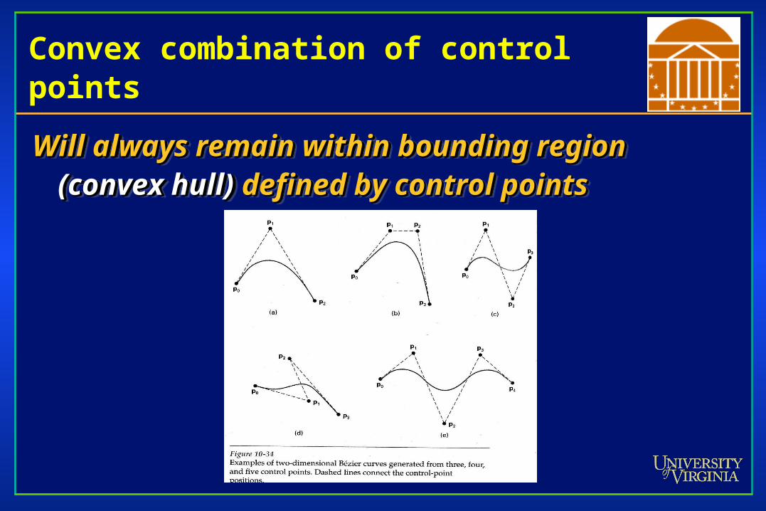
Will always remain within bounding region Will always remain within bounding region (convex hull)(convex hull) defined by control points defined by control points
Will always remain within bounding region Will always remain within bounding region (convex hull)(convex hull) defined by control points defined by control points

Bézier Curves
BezierBezierBezierBezier
Why more spline slides?
Bezier and Hermite splines have global influenceBezier and Hermite splines have global influence• One could create a Bezier curve that required 15 points to define the One could create a Bezier curve that required 15 points to define the
curve…curve…
– Moving any one control point would affect the entire curveMoving any one control point would affect the entire curve
• Piecewise Bezier or Hermite don’t suffer from this, but they don’t Piecewise Bezier or Hermite don’t suffer from this, but they don’t enforce derivative continuity at join pointsenforce derivative continuity at join points
B-splinesB-splines consist of curve segments whose polynomial consist of curve segments whose polynomial coefficients depend on just a few control pointscoefficients depend on just a few control points• Local controlLocal control
Examples of SplinesExamples of Splines
B-Spline Curve (cubic periodic)
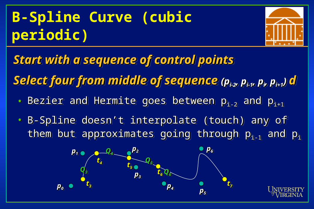
Start with a sequence of control pointsStart with a sequence of control points
Select four from middle of sequence Select four from middle of sequence (p(pi-2i-2, p, pi-1i-1, p, pii, p, pi+1i+1) ) dd
• Bezier and Hermite goes between pBezier and Hermite goes between p i-2i-2 and p and pi+1i+1
• B-Spline doesn’t interpolate (touch) any of them but B-Spline doesn’t interpolate (touch) any of them but approximates going through papproximates going through p i-1i-1 and p and pii
pp00pp00 pp44pp44
pp22pp22pp11pp11
pp33pp33
pp55pp55
pp66pp66
QQ33QQ33
QQ44QQ44
QQ55QQ55
QQ66QQ66
tt33tt33
tt44tt44 tt55tt55
tt66tt66
tt77tt77
Uniform B-Splines
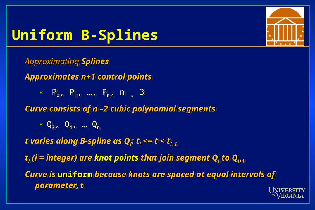
ApproximatingApproximating Splines Splines
Approximates n+1 control pointsApproximates n+1 control points
• PP00, P, P11, …, P, …, Pnn, n , n ¸̧ 3 3
Curve consists of n –2 cubic polynomial segmentsCurve consists of n –2 cubic polynomial segments
• QQ33, Q, Q44, … Q, … Qnn
t varies along B-spline as Qt varies along B-spline as Qii: t: tii <= t < t <= t < ti+1i+1
ttii (i = integer) are (i = integer) are knot pointsknot points that join segment Q that join segment Qii to Q to Qi+1i+1
Curve is Curve is uniformuniform because knots are spaced at equal intervals of because knots are spaced at equal intervals of parameter,parameter, tt
Uniform B-Splines
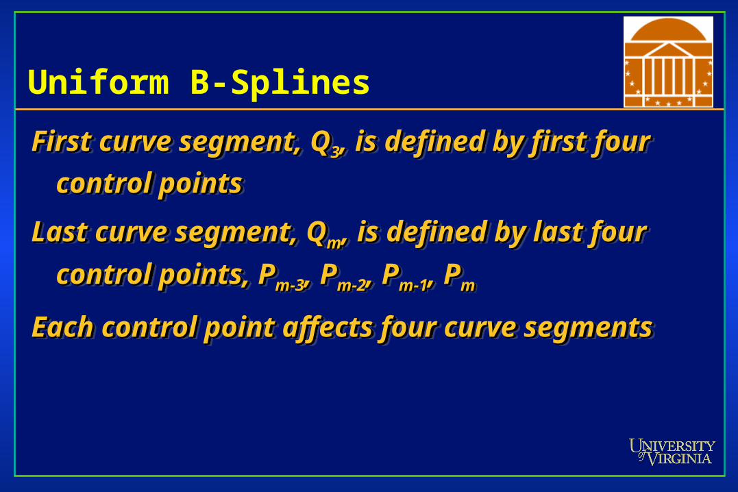
First curve segment, QFirst curve segment, Q33, is defined by first four , is defined by first four
control pointscontrol points
Last curve segment, QLast curve segment, Qmm, is defined by last four , is defined by last four
control points, Pcontrol points, Pm-3m-3, P, Pm-2m-2, P, Pm-1m-1, P, Pmm
Each control point affects four curve segmentsEach control point affects four curve segments
B-spline Basis Matrix
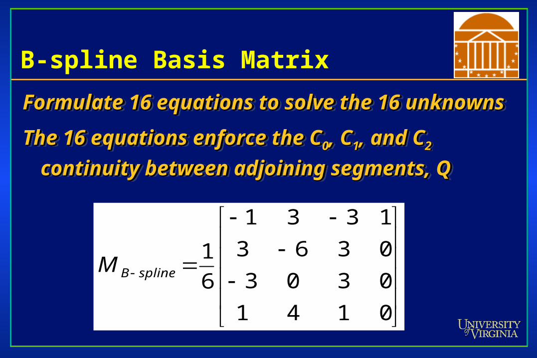
Formulate 16 equations to solve the 16 unknownsFormulate 16 equations to solve the 16 unknowns
The 16 equations enforce the CThe 16 equations enforce the C00, C, C11, and C, and C22
continuity between adjoining segments, Qcontinuity between adjoining segments, Q
Formulate 16 equations to solve the 16 unknownsFormulate 16 equations to solve the 16 unknowns
The 16 equations enforce the CThe 16 equations enforce the C00, C, C11, and C, and C22
continuity between adjoining segments, Qcontinuity between adjoining segments, Q
0141
0303
0363
1331
6
1splineBM
B-Spline
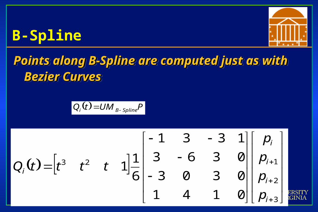
Points along B-Spline are computed just as with Points along B-Spline are computed just as with Bezier CurvesBezier Curves
Points along B-Spline are computed just as with Points along B-Spline are computed just as with Bezier CurvesBezier Curves
PUMtQ SplineBi
3
2
123
0141
0303
0363
1331
6
11
i
i
i
i
i
p
p
p
p
ttttQ
B-Spline
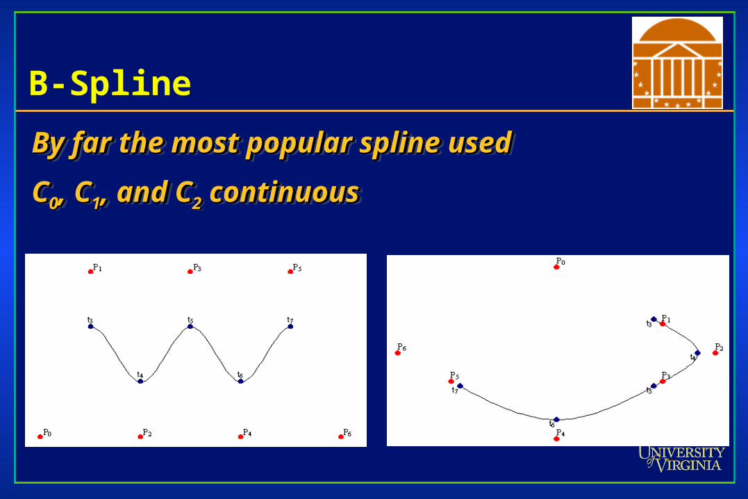
By far the most popular spline usedBy far the most popular spline used
CC00, C, C11, and C, and C22 continuous continuous
By far the most popular spline usedBy far the most popular spline used
CC00, C, C11, and C, and C22 continuous continuous
Nonuniform, Rational B-Splines(NURBS)
The native geometry element in MayaThe native geometry element in Maya
Models are composed of surfaces defined by Models are composed of surfaces defined by NURBS, not polygonsNURBS, not polygons
NURBS are smoothNURBS are smooth
NURBS require effort to make non-smoothNURBS require effort to make non-smooth
Converting Between Splines
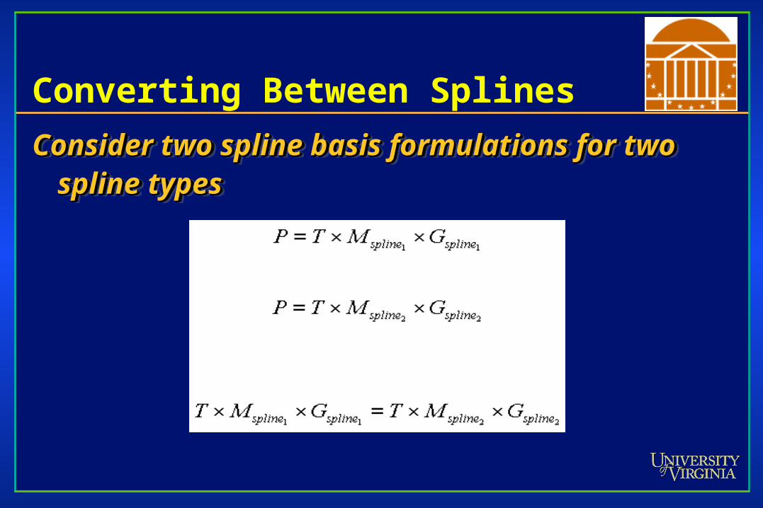
Consider two spline basis formulations for two Consider two spline basis formulations for two spline typesspline types
Consider two spline basis formulations for two Consider two spline basis formulations for two spline typesspline types
Converting Between Splines
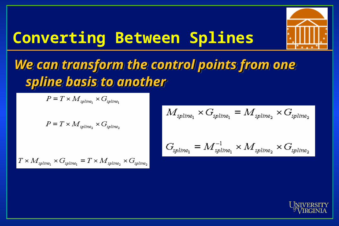
We can transform the control points from one We can transform the control points from one spline basis to anotherspline basis to another
We can transform the control points from one We can transform the control points from one spline basis to anotherspline basis to another
Converting Between Splines
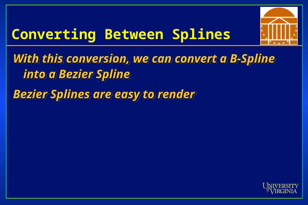
With this conversion, we can convert a B-Spline With this conversion, we can convert a B-Spline into a Bezier Splineinto a Bezier Spline
Bezier Splines are easy to renderBezier Splines are easy to render
With this conversion, we can convert a B-Spline With this conversion, we can convert a B-Spline into a Bezier Splineinto a Bezier Spline
Bezier Splines are easy to renderBezier Splines are easy to render
Rendering Splines
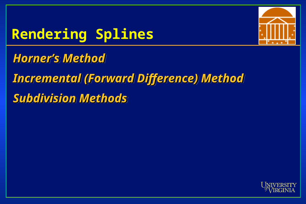
Horner’s MethodHorner’s Method
Incremental (Forward Difference) MethodIncremental (Forward Difference) Method
Subdivision MethodsSubdivision Methods
Horner’s MethodHorner’s Method
Incremental (Forward Difference) MethodIncremental (Forward Difference) Method
Subdivision MethodsSubdivision Methods
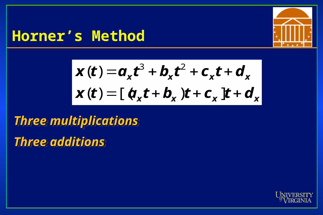
Horner’s Method
Three multiplicationsThree multiplications
Three additionsThree additions
Three multiplicationsThree multiplications
Three additionsThree additions
xxxx
xxxx
dtctbtatx
dtctbtatx
])[()(
)( 23
Forward Difference
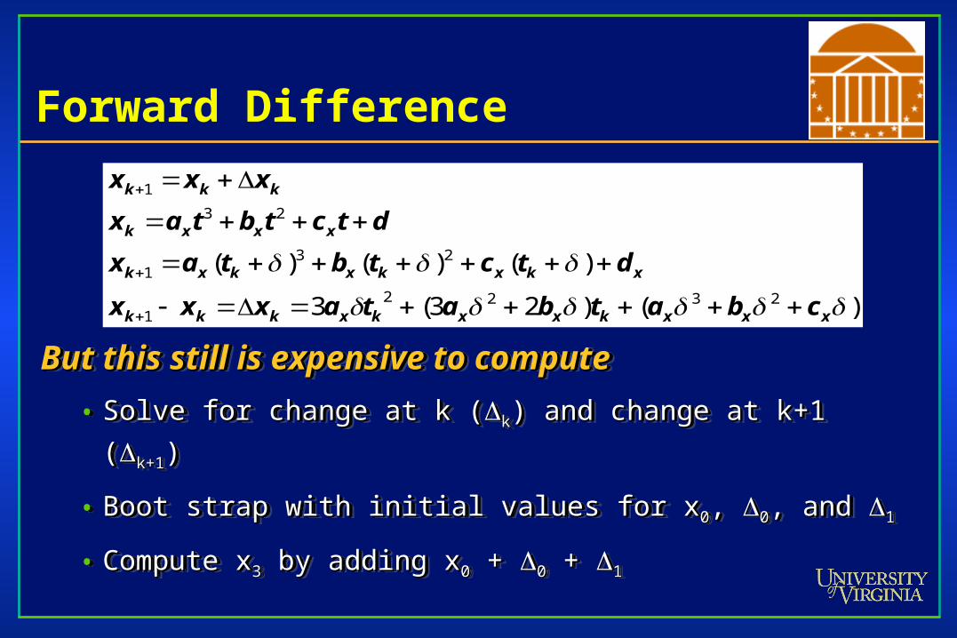
But this still is expensive to computeBut this still is expensive to compute
• Solve for change at k (Solve for change at k (kk) and change at k+1 () and change at k+1 (k+1k+1))
• Boot strap with initial values for xBoot strap with initial values for x00, , 00, and , and 11
• Compute xCompute x33 by adding x by adding x00 + + 00 + + 11
)()23(3
)()()(2322
1
231
23
1
xxxkxxkxkkk
xkxkxkxk
xxxk
kkk
cbatbataxxx
dtctbtax
dtctbtax
xxx
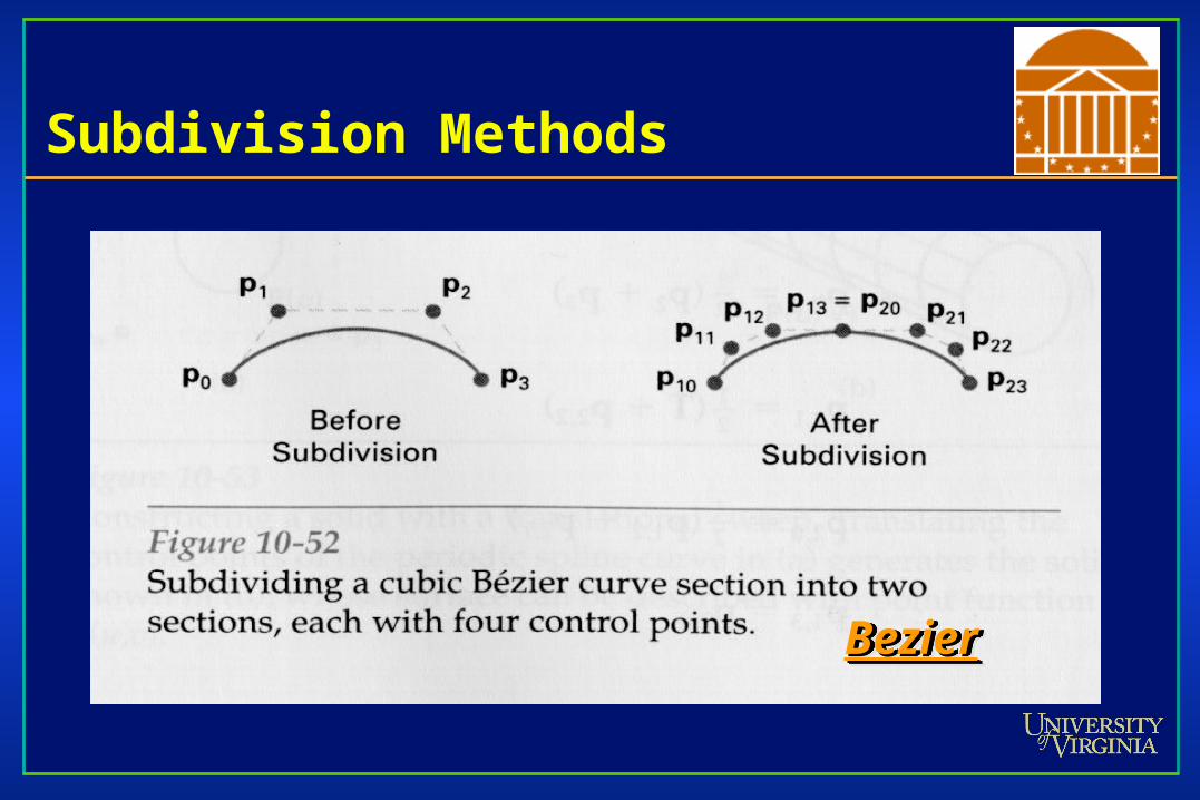
Subdivision Methods
BezierBezierBezierBezier
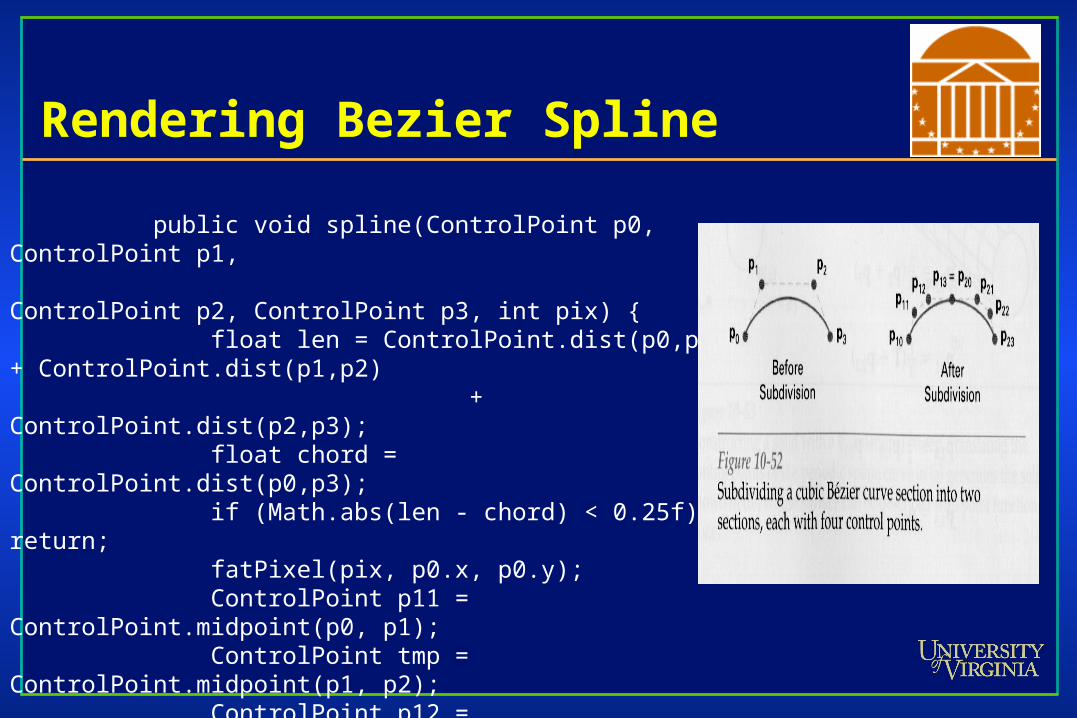
Rendering Bezier Spline
public void spline(ControlPoint p0, ControlPoint p1, ControlPoint p2, ControlPoint p3, int pix) { float len = ControlPoint.dist(p0,p1) + ControlPoint.dist(p1,p2) + ControlPoint.dist(p2,p3); float chord = ControlPoint.dist(p0,p3); if (Math.abs(len - chord) < 0.25f) return; fatPixel(pix, p0.x, p0.y); ControlPoint p11 = ControlPoint.midpoint(p0, p1); ControlPoint tmp = ControlPoint.midpoint(p1, p2); ControlPoint p12 = ControlPoint.midpoint(p11, tmp); ControlPoint p22 = ControlPoint.midpoint(p2, p3); ControlPoint p21 = ControlPoint.midpoint(p22, tmp); ControlPoint p20 = ControlPoint.midpoint(p12, p21); spline(p20, p12, p11, p0, pix); spline(p3, p22, p21, p20, pix); }

Do you want a 5th assignment?

Assignment 5
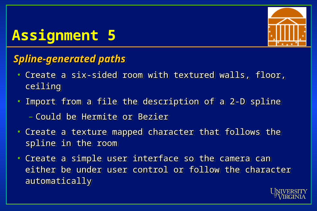
Spline-generated pathsSpline-generated paths
• Create a six-sided room with textured walls, floor, ceilingCreate a six-sided room with textured walls, floor, ceiling
• Import from a file the description of a 2-D splineImport from a file the description of a 2-D spline
– Could be Hermite or BezierCould be Hermite or Bezier
• Create a texture mapped character that follows the spline in Create a texture mapped character that follows the spline in the roomthe room
• Create a simple user interface so the camera can either be Create a simple user interface so the camera can either be under user control or follow the character automaticallyunder user control or follow the character automatically
Virtual Trackball
Can we use the mouse to control the 2-D rotation Can we use the mouse to control the 2-D rotation of a viewing volume?of a viewing volume?
Imagine a track ballImagine a track ball
• User moves point on ball from (x, y, z) to (a, b, c)User moves point on ball from (x, y, z) to (a, b, c)
Imagine the points projected onto the groundImagine the points projected onto the ground
• User moves point on ground from (x, 0, z) to (a, 0, c)User moves point on ground from (x, 0, z) to (a, 0, c)
Trackball
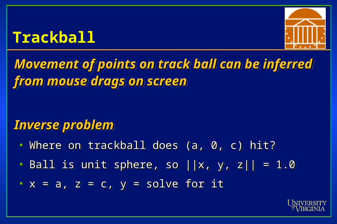
Movement of points on track ball can be inferred Movement of points on track ball can be inferred from mouse drags on screenfrom mouse drags on screen
Inverse problemInverse problem
• Where on trackball does (a, 0, c) hit?Where on trackball does (a, 0, c) hit?
• Ball is unit sphere, so ||x, y, z|| = 1.0Ball is unit sphere, so ||x, y, z|| = 1.0
• x = a, z = c, y = solve for itx = a, z = c, y = solve for it
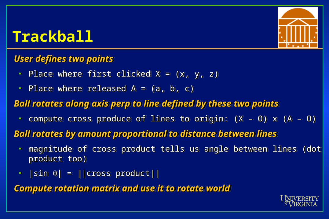
TrackballUser defines two pointsUser defines two points
• Place where first clicked X = (x, y, z)Place where first clicked X = (x, y, z)
• Place where released A = (a, b, c)Place where released A = (a, b, c)
Ball rotates along axis perp to line defined by these two pointsBall rotates along axis perp to line defined by these two points
• compute cross produce of lines to origin: (X – O) x (A – O)compute cross produce of lines to origin: (X – O) x (A – O)
Ball rotates by amount proportional to distance between linesBall rotates by amount proportional to distance between lines
• magnitude of cross product tells us angle between lines (dot product too)magnitude of cross product tells us angle between lines (dot product too)
• |sin |sin | = ||cross product||| = ||cross product||
Compute rotation matrix and use it to rotate worldCompute rotation matrix and use it to rotate world
User defines two pointsUser defines two points
• Place where first clicked X = (x, y, z)Place where first clicked X = (x, y, z)
• Place where released A = (a, b, c)Place where released A = (a, b, c)
Ball rotates along axis perp to line defined by these two pointsBall rotates along axis perp to line defined by these two points
• compute cross produce of lines to origin: (X – O) x (A – O)compute cross produce of lines to origin: (X – O) x (A – O)
Ball rotates by amount proportional to distance between linesBall rotates by amount proportional to distance between lines
• magnitude of cross product tells us angle between lines (dot product too)magnitude of cross product tells us angle between lines (dot product too)
• |sin |sin | = ||cross product||| = ||cross product||
Compute rotation matrix and use it to rotate worldCompute rotation matrix and use it to rotate world