Crude Oil Under Negative Pressures and Hydrocarbons Emission Containment M. Husain, (M) President, MH Systems, Inc., San Diego, CA H. Hunter, MH Systems, Inc. San Diego, CA D. Altshuller, MH Systems, Inc., San Diego, CA E. Shtepani, Hycal Energy Research Labs Ltd., Calgary, AB, Canada S. Luckhardt, Energy Research Center, University of California, San Diego, CA

ABSTRACT

This paper presents the results of experimental and theoretical analysis of crude oil under negative (sub-atmospheric) pressures. The use of negative pressure in the ullage space of tankers has been proposed for the mitigation of cargo losses resulting from accidental hull rupture. This potential application resulted in detailed laboratory tests of various crudes over a range of temperatures and pressures. The findings were then applied to prevent or minimize VOC (Volatile Organic Compound) emissions occurring during transport of crude oil. Equilibrium between liquid and gas/vapor components is reached at moderate hydrocarbon partial pressures. Predictions of liquid-vapor transformation can be made very accurately from known relationships, in the present case, the Peng-Robinson equation of state. The amount of material vaporized in reaching equilibrium is small, and the composition of the source liquid is changed only slightly. It can be shown that the partial pressures of hydrocarbon components are low, and can be accommodated by a closed system.

The adverse environmental and economic losses caused by VOC emissions from crude oil tankers are significant. A brief discussion on the design of a closed, negative pressure system for VOC emission minimization is discussed. The closed loop system, along with a seawater heat exchanger, mitigates the effects of temperature and pressures as well and will significantly reduce VOC venting to the atmosphere.

Mo molecular weight of liquid NOMENCLATURE Ma Mach number a, b constants in cubic equation of state P Pressure A, B, C constants in Antoine equation Q heat load C ullage capacity coefficient Q(s) volume flow rate in the Laplace domain Cp specific heat Q& heat flow rate BTU/sec D duct diameter R gas constant hD turbulent heat transfer coefficient 5.4 BTU/hr

ft2 oF for a flow speed of 30 ft/sec. s Laplace-domain variable S entropy H enthalpy t time K control loop gain T temperature L duct length Tinlet(t) inlet gas temperature m& gas mass flow Tw wall temperature

Mg molecular weight of gas Tx gas temperature at distance x Mi molecular weight of ith component

1

∆T temperature rise oF. loading. Therefore, VOC evaporation continues during transit. A closed-system equilibrium (at saturation) may not be reached because of frequent venting and inerting.

V volume xi molar fraction of a component in liquid phase

Diurnal heating and cooling of the cargo tanks increases the variation in ullage pressure necessitating additional venting and inerting. Under current management practice, periodic venting can continue during an entire voyage.

yi molar fraction of a component in gas phase Z thermodynamic compression factor Greek Letters

The concept to be discussed in this paper is to contain in-transit VOC emissions by maintaining a near constant ullage pressure. Ullage gases are circulated in a closed-loop arrangement at sub-atmospheric pressure via a blower and seawater heat exchanger. It is the circulation that makes it possible to maintain constant ullage pressure under perturbations caused by mass and heat transfer during the voyage. The system can be implemented at moderate cost and with the use of essentially standard marine components.

γ specific heat ratio ε emissivity κ thermodynamic constant ρ density

SBσ Stefan-Boltzman constant ω acentric factor Ω thermodynamic constant INTRODUCTION Part 1 presents a summary of the laboratory tests

conducted in order to define crude oil vaporization processes under moderately reduced pressures. The laboratory test data formed the basis for the development of an equation of state model. This model allows the test data to be extrapolated to conditions that were not explicitly present in the tests.

The transport of crude oil by sea represents a continuing source of pollution by cargo loss due to collision and grounding and by venting of volatile organic compounds (VOC) evolved from the cargo. Cargo losses due to collision and grounding have been estimated at about 25,000 tons per year, with occasional catastrophic losses. INTERTANKO (Gunner 1999) estimates losses of VOC to the atmosphere at about 1.6 million tons per year. Other estimates put this number at 4 million tons or more per year.

A brief reference is made to a full-scale tanker test of a reduced ullage pressure system. The test (Husain et al 2001) demonstrated that the proposed pressure control system could be implemented and managed without undue cost or operational difficulty. The final section presents a brief description and proof-of-concept evaluation of an operating system for crude oil tankers satisfying these requirements:

Over the past several years, the authors have been conducting research, testing and conceptual design of ullage gas/vapor management systems. Primarily, these studies have focused on containment of oil spills by maintaining subatmospheric ullage pressure.

• Contain VOC emissions by eliminating the

need for venting or topping, as currently practiced in tanker transport.

However, these studies have also demonstrated a collateral benefit that can be achieved by maintaining constant ullage pressure - a practical approach to the reduction of VOC emissions.

• Sustain saturated conditions in the ullage gases

throughout the voyage. It is currently required that the ullage space be (i) suitably inerted, normally using oxygen-depleted flue gas, and (ii) that the pressure be maintained at a positive value, typically about 1.5 psig. At the same time, it is also required that ullage pressure may not exceed a given level, typically about 2 psig.

• Provide for a wider pressure excursion band

by operating at moderate sub-atmospheric pressures.

These pressure bounds are close together, requiring that a nearly constant pressure be maintained between them. Pressure excursions beyond these limits require either venting or the addition of inert gas. This need can be reduced or eliminated if subatmospheric pressure is maintained in the ullage, because then the margin between the pressure bounds increases.

• Minimize pressure fluctuations resulting from mass and heat transfer in the ullage spaces.

It is recognized that the reduction of the lower pressure bound from 1.5 psig to subatmospheric level would conflict with current regulations for tankers, and would thus require careful development, qualification testing and regulatory approval. The ullage mixture is generally not in equilibrium

with the liquid cargo at the completion of cargo

2

3

PART I – ANALYSIS OF CRUDE OIL UNDER NEGATIVE PRESSURES Overview

An experimental study, together with a theoretical analysis, was conducted to determine the vaporization properties of representative crude oil samples at pressures below atmospheric and at the moderately elevated temperatures typical of crude oil transport at sea. This section of the report summarizes these investigations. In brief, the experimental phase placed a sample of the as-received crude in a closed container under an inert gas atmosphere. Temperature was maintained at a predetermined level, and pressure was set to a specified value by adding inert gas or by removing the mixture. When equilibrium had been obtained, pressures, temperatures and liquid and vapor compositions were measured. In the experiments the ullage volume was 25% of the total volume. By applying the equations of state (see Appendix 2) the results for any volume of the ullage space can be predicted. These data were fitted to appropriate theoretical relationships in order to verify that vapor composition was related to liquid composition in accordance with theory. The correspondence was excellent. The observed test points were also compared to predictions made using a computer-based equation of state (EOS) model. In this case, too, the observations corresponded closely with predictions. These operations are described in the following sections. The conclusions derived from the laboratory tests and analyses are as follows:

• Steady-state equilibrium between the liquid and gas/vapor components is reached at very moderate partial pressures of hydrocarbon mixture. The amount vaporized increases as the temperature increases and as ambient pressure decreases.

• The amount vaporized will adjust in either

direction as temperature or pressure change.

• The composition of the vapor mixture is essentially as predicted analytically, based on the liquid composition.

• This prediction can be made very accurately

from known relationships using a computer

model to carry out the calculations. In the present case, the Peng-Robinson equation of state, a relation frequently used in the petroleum industry, correlated very well with test data.

• The amount of material vaporized in reaching

equilibrium is very small, and the composition of the source liquid is changed only slightly. In relation to the transport of crude, if pressure can be held constant this vaporized material is a one-time loss of cargo, not a continuing one.

Experimental Work

To measure gas evolution from the crude oil at reduced pressures and at given temperature, the following procedure was performed:

• While purging the autoclave mixer with nitrogen, pour in 75 % in volume the crude oil to be tested.

• Seal the mixer with appropriate valves and

gauges.

• At zero psig and lab temperature, after stabilization, measure a small gas analysis (about 50cc is required), being careful not to pull a negative pressure.

• To achieve the reduced pressures, a sampling

syringe is used. The syringe is pre-purged with helium and evacuated.

• The volume of gas taken is measured in the

gasometer and analyzed for composition using Gas Chromatograph.

This procedure is repeated for every pressure stage and at given temperature. Always the system is isolated and the temperature is stabilized, then the syringe is used to obtain the reduced pressure. The schematic of equipment used is shown in Figure 1.

Three crude oils were selected, which cover the range from 12 API to 37 API. The compositional analyses of crude oils were performed. For each of them a series of gas evolution tests was performed at pressures of 0 psig, -2 psig, -3 psig and –5 psig at temperatures 67 F, 80 F and 110 F and the liberated gas compositions were measured.

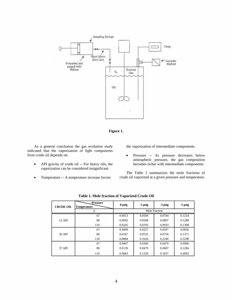
Figure 1.

As a general conclusion the gas evolution study indicated that the vaporization of light components from crude oil depends on:

• API gravity of crude oil -- For heavy oils, the

vaporization can be considered insignificant. • Temperature -- A temperature increase favors

the vaporization of intermediate components.

• Pressure -- As pressure decreases below atmospheric pressure, the gas composition becomes richer with intermediate components.

The Table 1 summarizes the mole fractions of

crude oil vaporized at a given pressure and temperature.

Table 1. Mole fraction of Vaporized Crude Oil

Pressure Temperature 0 psig -2 psig -3 psig -5 psig

F67 0.0013 0.0500 0.0744 0.1234

12 API 80 0.0092 0.0568 0.0807 0.1288110 0.0245 0.0703 0.0933 0.139867 0.0009 0.0327 0.0507 0.0956

30 API 80 0.0167 0.0535 0.0756 0.1371110 0.0868 0.1626 0.2240 0.529867 0.0007 0.0300 0.0470 0.0906

37 API 80 0.0139 0.0479 0.0687 0.1284

110 0.0683 0.1329 0.1837 0.4093

CRUDE OILMole Fraction

4

The vaporization described above is in accordance with expectations. In terms of quantity, even in the worst-case scenario of highest temperature and lowest pressure, the amount of vaporised components was within 0.55% in mole, as shown in Table 1. That means that the change in the crude oil composition is practically insignificant. A detailed explanation of mechanism and compositional description of oils exposed to volatility and extraction processes is described in the technical paper of F.B. Thomas et al.

A summary of each crude oil compositions tested at stock tank conditions and after the highest vaporization (highest temperature and lowest pressure) has occurred is given in Appendix 1.

The differences in the composition before and after the process of vaporization are practically within the error of chromatography measurements. This is a good indicator that the properties of crude oil are not affected by this degree of vaporization. On the other side, because the gas vaporised remains in equilibrium with

the crude oil, depending on conditions the evaporants may again go into solution either partially or fully.

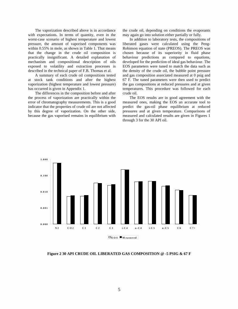
In addition to laboratory tests, the compositions of liberated gases were calculated using the Peng-Robinson equation of state (PREOS). The PREOS was chosen because of its superiority in fluid phase behaviour predictions as compared to equations, developed for the prediction of ideal gas behaviour. The EOS parameters were tuned to match the data such as the density of the crude oil, the bubble point pressure and gas composition associated measured at 0 psig and 67 F. The tuned parameters were then used to predict the gas compositions at reduced pressures and at given temperatures. This procedure was followed for each crude oil.

The EOS results are in good agreement with the measured ones, making the EOS an accurate tool to predict the gas-oil phase equilibrium at reduced pressures and at given temperature. Comparisons of measured and calculated results are given in Figures 1 through 3 for the 30 API oil.

0 .0 0 0

0 .0 0 1

0 .0 1 0

0 .1 0 0

1 .0 0 0

N 2 C O 2 C 1 C 2 C 3 i- C 4 n - C 4 i- C 5 n - C 5 C 6 C 7 +

E O S M e a s u r e d

Figure 2 30 API CRUDE OIL LIBERATED GAS COMPOSITION @ -5 PSIG & 67 F

5

0.000

0.001

0.010

0.100

1.000

N2 CO2 C1 C2 C3 i-C4 n-C4 i-C5 n-C5 C6 C7+

EOS Measured

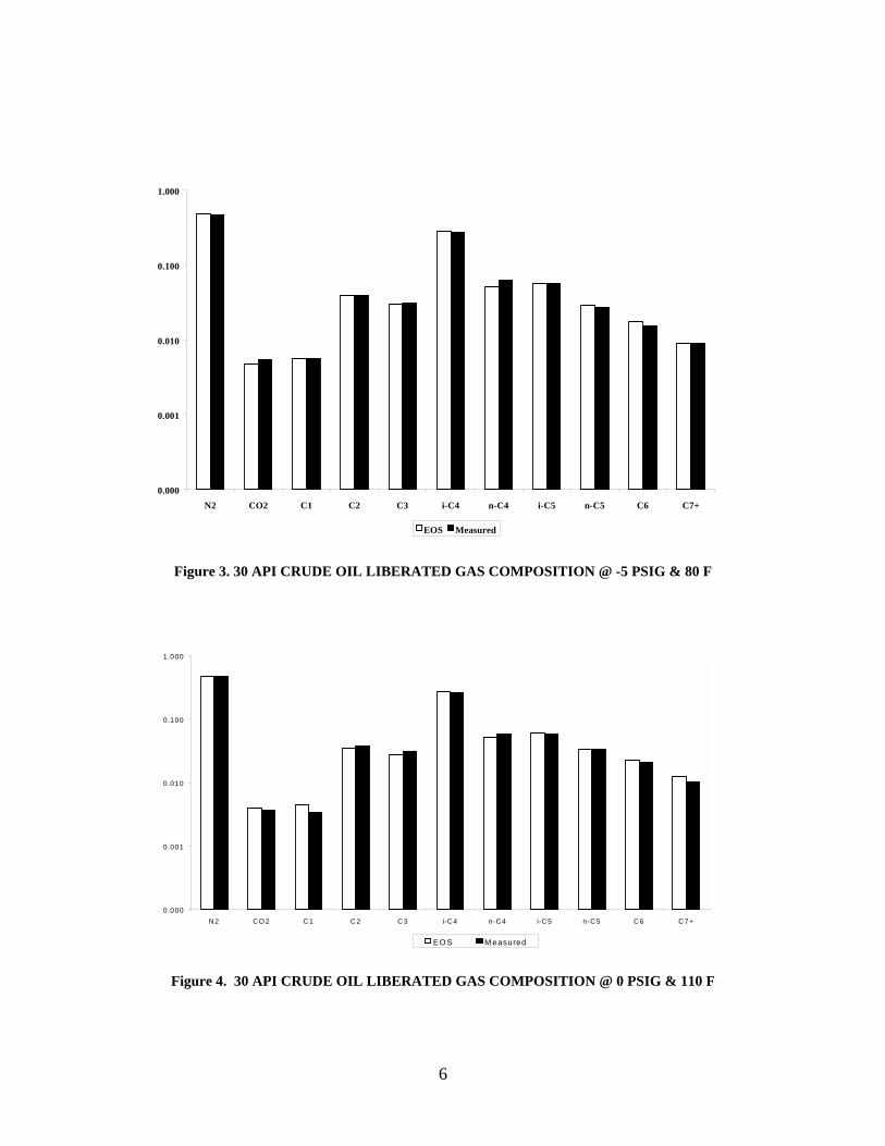
Figure 3. 30 API CRUDE OIL LIBERATED GAS COMPOSITION @ -5 PSIG & 80 F

0.000

0.001

0.010

0.100

1.000

N 2 C O 2 C 1 C 2 C 3 i-C 4 n-C4 i-C 5 n-C5 C 6 C 7+

EO S M easured

Figure 4. 30 API CRUDE OIL LIBERATED GAS COMPOSITION @ 0 PSIG & 110 F

6

A summarized description of EOS characterization and calculation techniques used is given in Appendix 2.

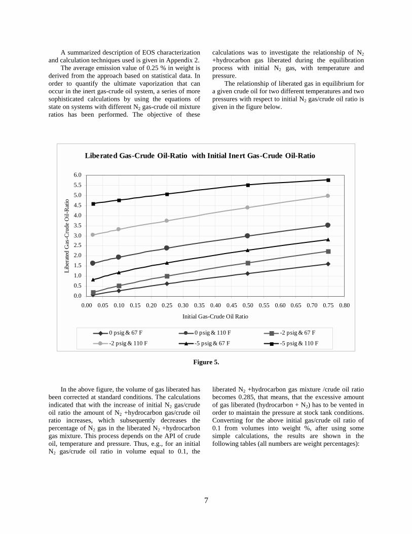
The average emission value of 0.25 % in weight is derived from the approach based on statistical data. In order to quantify the ultimate vaporization that can occur in the inert gas-crude oil system, a series of more sophisticated calculations by using the equations of state on systems with different N2 gas-crude oil mixture ratios has been performed. The objective of these

calculations was to investigate the relationship of N2 +hydrocarbon gas liberated during the equilibration process with initial N2 gas, with temperature and pressure.

The relationship of liberated gas in equilibrium for a given crude oil for two different temperatures and two pressures with respect to initial N2 gas/crude oil ratio is given in the figure below.

Liberated Gas-Crude Oil-Ratio with Initial Inert Gas-Crude Oil-Ratio

0.0

0.5

1.0

1.5

2.0

2.53.0

3.5

4.0

4.5

5.0

5.5

6.0

0.00 0.05 0.10 0.15 0.20 0.25 0.30 0.35 0.40 0.45 0.50 0.55 0.60 0.65 0.70 0.75 0.80

Initial Gas-Crude Oil Ratio

Libe

rate

d G

as-C

rude

Oil-

Rat

io

0 psig & 67 F 0 psig & 110 F -2 psig & 67 F

-2 psig & 110 F -5 psig & 67 F -5 psig & 110 F

Figure 5.

In the above figure, the volume of gas liberated has been corrected at standard conditions. The calculations indicated that with the increase of initial N2 gas/crude oil ratio the amount of N2 +hydrocarbon gas/crude oil ratio increases, which subsequently decreases the percentage of N2 gas in the liberated N2 +hydrocarbon gas mixture. This process depends on the API of crude oil, temperature and pressure. Thus, e.g., for an initial N2 gas/crude oil ratio in volume equal to 0.1, the

liberated N2 +hydrocarbon gas mixture /crude oil ratio becomes 0.285, that means, that the excessive amount of gas liberated (hydrocarbon + N2) has to be vented in order to maintain the pressure at stock tank conditions. Converting for the above initial gas/crude oil ratio of 0.1 from volumes into weight %, after using some simple calculations, the results are shown in the following tables (all numbers are weight percentages):

7

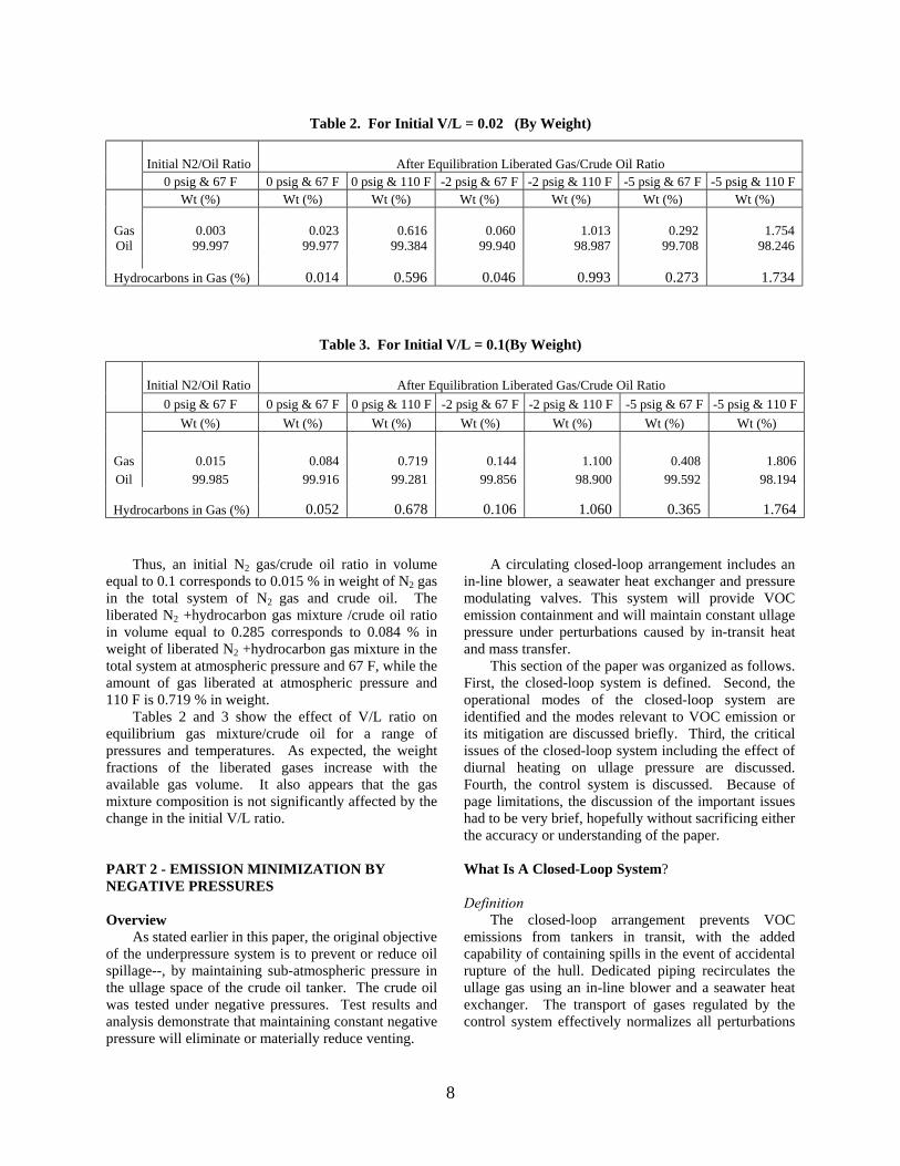
Table 2. For Initial V/L = 0.02 (By Weight)

Initial N2/Oil Ratio After Equilibration Liberated Gas/Crude Oil Ratio

0 psig & 67 F 0 psig & 67 F 0 psig & 110 F -2 psig & 67 F -2 psig & 110 F -5 psig & 67 F -5 psig & 110 F Wt (%) Wt (%) Wt (%) Wt (%) Wt (%) Wt (%) Wt (%) Gas 0.003 0.023 0.616 0.060 1.013 0.292 1.754 Oil 99.997 99.977 99.384 99.940 98.987 99.708 98.246

Hydrocarbons in Gas (%) 0.014 0.596 0.046 0.993 0.273 1.734

Table 3. For Initial V/L = 0.1(By Weight)

Initial N2/Oil Ratio After Equilibration Liberated Gas/Crude Oil Ratio

0 psig & 67 F 0 psig & 67 F 0 psig & 110 F -2 psig & 67 F -2 psig & 110 F -5 psig & 67 F -5 psig & 110 F Wt (%) Wt (%) Wt (%) Wt (%) Wt (%) Wt (%) Wt (%) Gas 0.015 0.084 0.719 0.144 1.100 0.408 1.806 Oil 99.985 99.916 99.281 99.856 98.900 99.592 98.194

Hydrocarbons in Gas (%) 0.052 0.678 0.106 1.060 0.365 1.764

Thus, an initial N2 gas/crude oil ratio in volume

equal to 0.1 corresponds to 0.015 % in weight of N2 gas in the total system of N2 gas and crude oil. The liberated N2 +hydrocarbon gas mixture /crude oil ratio in volume equal to 0.285 corresponds to 0.084 % in weight of liberated N2 +hydrocarbon gas mixture in the total system at atmospheric pressure and 67 F, while the amount of gas liberated at atmospheric pressure and 110 F is 0.719 % in weight.

Tables 2 and 3 show the effect of V/L ratio on equilibrium gas mixture/crude oil for a range of pressures and temperatures. As expected, the weight fractions of the liberated gases increase with the available gas volume. It also appears that the gas mixture composition is not significantly affected by the change in the initial V/L ratio. PART 2 - EMISSION MINIMIZATION BY NEGATIVE PRESSURES Overview

As stated earlier in this paper, the original objective of the underpressure system is to prevent or reduce oil spillage--, by maintaining sub-atmospheric pressure in the ullage space of the crude oil tanker. The crude oil was tested under negative pressures. Test results and analysis demonstrate that maintaining constant negative pressure will eliminate or materially reduce venting.

A circulating closed-loop arrangement includes an in-line blower, a seawater heat exchanger and pressure modulating valves. This system will provide VOC emission containment and will maintain constant ullage pressure under perturbations caused by in-transit heat and mass transfer. This section of the paper was organized as follows. First, the closed-loop system is defined. Second, the operational modes of the closed-loop system are identified and the modes relevant to VOC emission or its mitigation are discussed briefly. Third, the critical issues of the closed-loop system including the effect of diurnal heating on ullage pressure are discussed. Fourth, the control system is discussed. Because of page limitations, the discussion of the important issues had to be very brief, hopefully without sacrificing either the accuracy or understanding of the paper. What Is A Closed-Loop System? Definition The closed-loop arrangement prevents VOC emissions from tankers in transit, with the added capability of containing spills in the event of accidental rupture of the hull. Dedicated piping recirculates the ullage gas using an in-line blower and a seawater heat exchanger. The transport of gases regulated by the control system effectively normalizes all perturbations

8

in-transit that could change underpressure or inertness of the ullage gases. It is important to distinguish the term “closed-loop” used to describe the underpressure system arrangement from the one commonly used in control engineering. The former refers to the fact that the ullage gases are recirculated through the system as opposed to venting to the atmosphere or to the vapor recovery facility (open-loop arrangement). The loop regulating the ullage and the header pressure (described later in this paper) is always closed in the sense of control engineering.

In the closed-loop underpressure system, negative pressure must be maintained at a predetermined level to prevent cargo loss in the event of accident, while oxygen content must be held within specified limits to eliminate fire danger. Inert ullage gases are circulated through the ullage spaces, primarily to dilute air that could leak into the reduced-pressure ullage spaces, and the gases are returned to the tanks via a blower and seawater heat exchanger. The blower compensates for the pressure loss during transfer and the heat exchanger keeps the gas/vapor temperature low.

All piping, components and controls are independent of the tanker supporting services. There are other operational modes employed in contingencies and side-breaches that employ an open-loop configuration with an inert gas supply. These operational modes still contain spills, but not VOC emissions.

The ullage pressure is maintained between –2 and –3 psi (set pressure). This is accomplished by controlling the flow rate through the blower and by restricting the flow into each tank through the inlet valve. The ullage pressure is continuously monitored.

The controller (including both hardware and software) is designed to respond to pressure perturbations resulting from mass (from leakage or evaporation) and heat transfer in a circulating closed-loop system.

Operational Modes The underpressure system is designed to operate in the following modes:

Mode 0. Cargo loading Mode 1. Initial reduction of ullage pressure -2 to -3 psi Mode 2. Normal transit Mode 3. Contingency when oxygen

concentration exceeds 5% but not 8% Mode 4. Contingency when oxygen

concentration exceeds 8% Mode 5. Grounding Mode 6. Grounding with strong tidal variations

Mode 7. Side damage of a cargo tank Mode 8. Routine cargo unloading at destination Mode 9. Cargo unloading in the event of a tank

damage.

In the operational mode 0 (cargo loading) the underpressure system is off line. The ship’s supply of inert gas is used to maintain the inert atmosphere in the cargo tank. Vapors are collected and transferred to a vapor recovery facility.

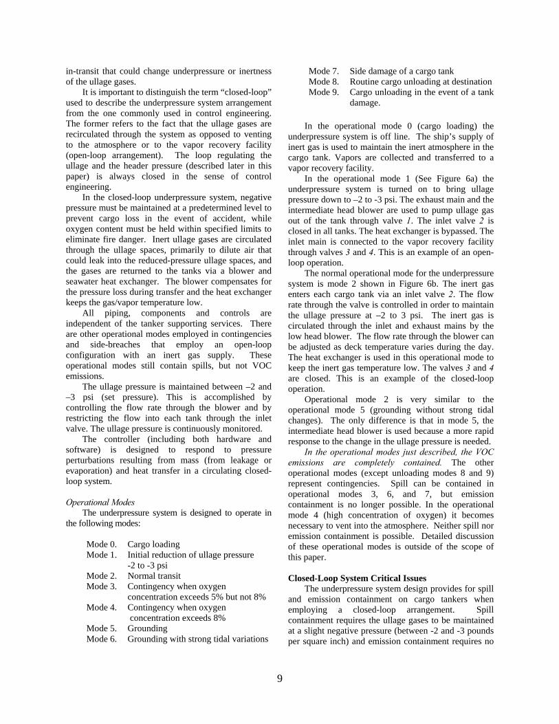
In the operational mode 1 (See Figure 6a) the underpressure system is turned on to bring ullage pressure down to –2 to -3 psi. The exhaust main and the intermediate head blower are used to pump ullage gas out of the tank through valve 1. The inlet valve 2 is closed in all tanks. The heat exchanger is bypassed. The inlet main is connected to the vapor recovery facility through valves 3 and 4. This is an example of an open-loop operation.

The normal operational mode for the underpressure system is mode 2 shown in Figure 6b. The inert gas enters each cargo tank via an inlet valve 2. The flow rate through the valve is controlled in order to maintain the ullage pressure at –2 to 3 psi. The inert gas is circulated through the inlet and exhaust mains by the low head blower. The flow rate through the blower can be adjusted as deck temperature varies during the day. The heat exchanger is used in this operational mode to keep the inert gas temperature low. The valves 3 and 4 are closed. This is an example of the closed-loop operation.

Operational mode 2 is very similar to the operational mode 5 (grounding without strong tidal changes). The only difference is that in mode 5, the intermediate head blower is used because a more rapid response to the change in the ullage pressure is needed.

In the operational modes just described, the VOC emissions are completely contained. The other operational modes (except unloading modes 8 and 9) represent contingencies. Spill can be contained in operational modes 3, 6, and 7, but emission containment is no longer possible. In the operational mode 4 (high concentration of oxygen) it becomes necessary to vent into the atmosphere. Neither spill nor emission containment is possible. Detailed discussion of these operational modes is outside of the scope of this paper.

Closed-Loop System Critical Issues

The underpressure system design provides for spill and emission containment on cargo tankers when employing a closed-loop arrangement. Spill containment requires the ullage gases to be maintained at a slight negative pressure (between -2 and -3 pounds per square inch) and emission containment requires no

9

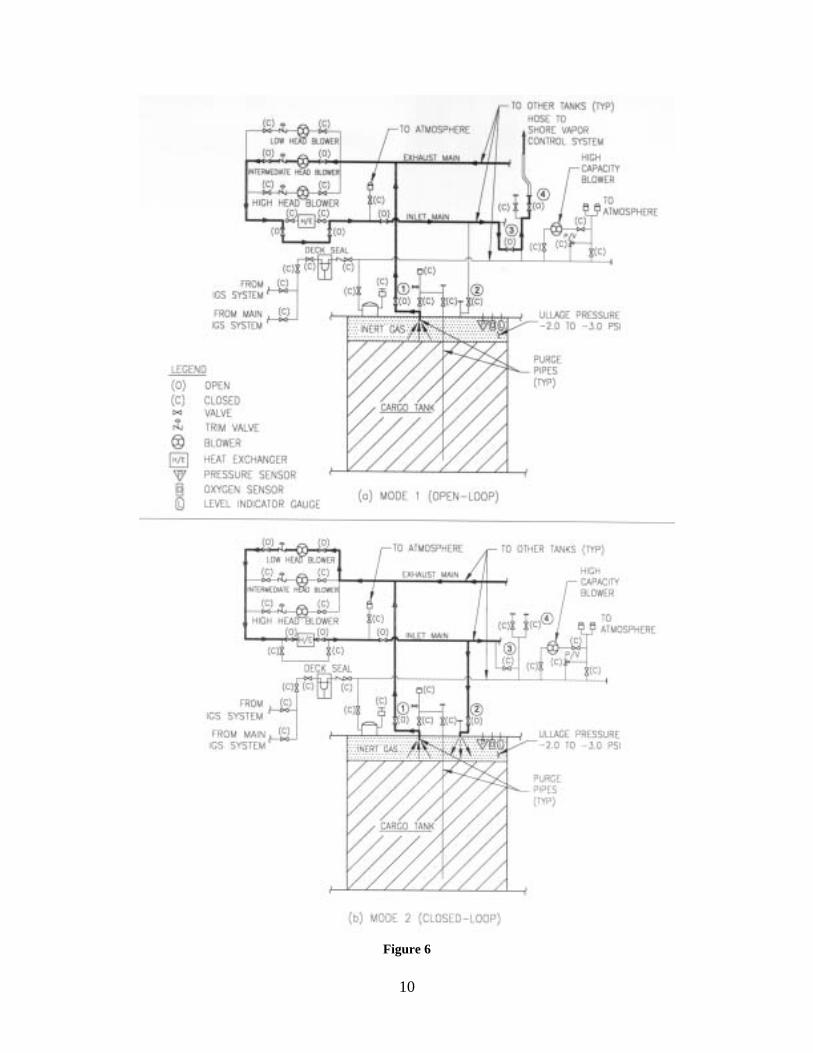
Figure 6

10

venting of the ullage gases during in-transit routine operations and during a grounding accident. The closed-loop arrangement essentially re-circulates the ullage gases at near seawater temperature while maintaining inertness by keeping oxygen content low. A number of “proof-of-concept” evaluations have been made in order to validate the key issues associated with the use of a closed-loop system. These are summarized below together with the improvements in cargo loss that are achieved: Potential Air Leakage and Its Contribution to Pressure and Oxygen Level Increases

Leakage estimates at the operational underpressure system was determined experimentally during full-scale testing aboard USNS Shoshone, a US Navy reserve fleet tanker. The effective leakage area derived from the test data at two pounds per square inch underpressure was less than 2 x 10-6 square feet. Leakage is most likely caused by the penetrations of ducting or instruments and is essentially independent of tank size. The observed leak, extrapolated for an ullage volume of 104 cubic feet, shows an increase of 1 psi over a 15-day voyage, for a closed non-circulating ullage volume. However, the appropriate controls of the circulating stream can still maintain the desired underpressure by adjusting the blower flow rate. Air leakage, based on field measurements, has a negligible effect on oxygen build-up over a 15-day voyage. However, the underpressure system provides a contingency mode, of an open-loop circulating stream,

that replenishes the ullage with fresh inert gas from a combustion gas generator to an oxygen level <5% by volume. This contingency mode is enabled when O2 levels are >5% by vol., through faulty assemblies or ducting stressed in high sea states. Negative Pressure Precludes the Need for Vapor Release or inert gas addition

Typically, tankers frequently add or release ullage gas/vapor. Venting occurs when the tank pressures approach a limit setting, which is 0.6 psi above the pressure lock-up at the completion of cargo loading (Figure 7). The frequency can reach every four hours. One plausible explanation for the pressure rise is the unsaturated condition of the ullage gases at the completion of cargo loading, with dissolved gases in the oil continuing to evolve to reach equilibrium (saturation), at a pressure in excess of the set venting pressure (16.2 psia).

This process of periodic venting will continue as long as the equilibrium pressure is in excess of the venting pressure. Diurnal heating further exacerbates these conditions. The underpressure system, on the other hand, draws down on the loading pressure and allows sufficient time for the gas to equilibrate, before setting the required underpressure. This setting is secured at -2 to –3 psi below the venting pressure so an ample excursion is available to the more volatile fluids if required. Venting will not be required with an enabled underpressure system.

Figure 7

11

Topping under current practice is required by the loss of positive ullage pressure through leakage to the atmosphere mainly due to poor fitting in the mast riser valving. If leakage occurs with the underpressure system the reverse happens, ullage pressure increases and the consequence is addressed. In any case, topping is not a required procedure with the underpressure system installation. In summary, both venting and topping will not be necessary with the underpressure system. Ullage Pressure Reduction due to Cargo Oil Cooling & Air Leakage Typically, cargo oil temperature decreases in transit due to heat transfer to the ocean. The hydrocarbon vapor pressure will accordingly decrease and reduce the total pressure of the gas mixture. The control’s modulating valves at the inlet to each tank effectively alters the flow rate into the ullage as required to maintain the underpressure. Diurnal Heating of Ullage Gas and its Effect on Ullage and Header Gas Pressure, Velocity, and Density There is a concern that heat input due to the sun’s radiant heat load could significantly raise the gas temperature and pressure adversely affecting the underpressure set for hydrostatic balance for spill control. A heat transfer analysis on the closed-loop underpressure system configuration installed on a large tanker operating on a mid-summer day in the Persian Gulf is addressed follows. The effect of temperature change on the pressure, velocity, and density can be calculated by using the following equations of gas dynamics (Zucrow and Hoffman 1976):

( )

TdTf

PdP MaMa 2γ= (1)

( )

TdTf

VdV Ma= (2)

( )

TdTfd Ma−=

ρρ (3)

In these equations Ma is the Mach number (the ratio of the gas flow speed to the speed of sound). The function f(Ma) has the property f(0)=1. Since the gas flows at a speed much slower than the speed of sound, it is reasonable to set Ma=0. Therefore, the right-hand side of the Equation (1) vanishes, and the conclusion is that temperature has no effect on gas pressure. From integration of the Equation (2) it follows that the speed of gas flow is directly proportional to the temperature. Gas density in the ullage can be determined

from the equations of state. Gas density in the header is determined by integrating Equation (3), which yields the conclusion that it is inversely proportional to temperature. The overall conclusion is that gas compressibility can be neglected for flow that is much slower than the speed of sound. Ullage gases exposed to the deck can reach as high as

F. However, this temperature change is not proportional to the pressure, as would occur in a closed non-circulating ullage space.

°165

A detailed analysis of the thermal load on the gas in both ullage and header is given in Appendix 3. The conclusion is that diurnal heating can be adequately addressed by a heat exchanger.

The control system includes a variable speed blower which can speed up to offset these losses, at no change in the circulating flow rate or ullage pressure. The in-line seawater heat exchanger removes the accumulation of heat deposited in the gas stream from the sun’s radiant heat and blower compression heat. Its size and pressure loss is moderate, and has a minimal effect on the design. VOC Emission Due to Loading Loading cargo in a tanker can be a primary source of emissions. These losses can be prevented by a vapor balance service or a shore vapor recovery system. These services would also reduce emissions occasioned by the initial depressurization in preparation for the voyage.

At the completion of loading at positive pressure, the hydrocarbon (HC) content is usually 30-40 percent by volume, which is approaching saturation. The ullage is now subject to depressurization to below atmospheric pressure, which causes the gas composition to become richer with additional outgassing to reach a saturation some 5% higher. This means a requirement for the vapor recovery facility to remain operable until the final adjustment to the preselected pressure is achieved and stabilized. In-transit, the saturated gases are circulated in a closed-loop arrangement consisting of an in-line blower, seawater heat exchanger and individual inlet valves to each tank that control flow to maintain tank pressure. The automated controls include the hardware, multiple sensors and software to ensure the underpressure is maintained through all operational perturbations. Tankers Structural Capability to Withstand Negative Pressures

Extensive theoretical analysis has been performed to determine the effects of negative pressures in ullage spaces of tanks, and strain gage tests were performed on the USNS Shoshone (a reserve fleet tanker) as well. Analysis (Mansour 1996) of 245,000 DWT VLCC

12

shows that even at –6 psig the increase in stresses was 9.4%. An analysis submitted by Japan (IMO 1993) for a 233,000 DWT tanker, shows that the negative pressure required to cause structural failure of the deck was found to be 19.8 psi (0.137 MPa). Strain gauge tests performed on the structures of the USNS Shoshone in 2001 show good correlation with mathematical models (Husain et al. 2001). Risk assessment A preliminary risk assessment was performed for the underpressure system in all of its operational phases. This analysis identified potential adverse events, frequency of occurrence, consequences if failure and possible mitigating measures.

As a result, the related design features include:

• An autonomous control system that ensures functional units and shipboard supporting services are operable, especially during a collision when the man/machine interface may not be fully available.

• Functional units are independent and separate

from ship’s systems, and are located where they are least susceptible to damage from a collision. The key units are the standby inert gas supply module, the electric/pneumatic power supply system, the gas distribution

• system and the controls and data transmission system.

• Design featuring redundancies and degraded

modes of operation built into the hardware and software systems, including dedicated inert gas generator.

CONTROL SYSTEM

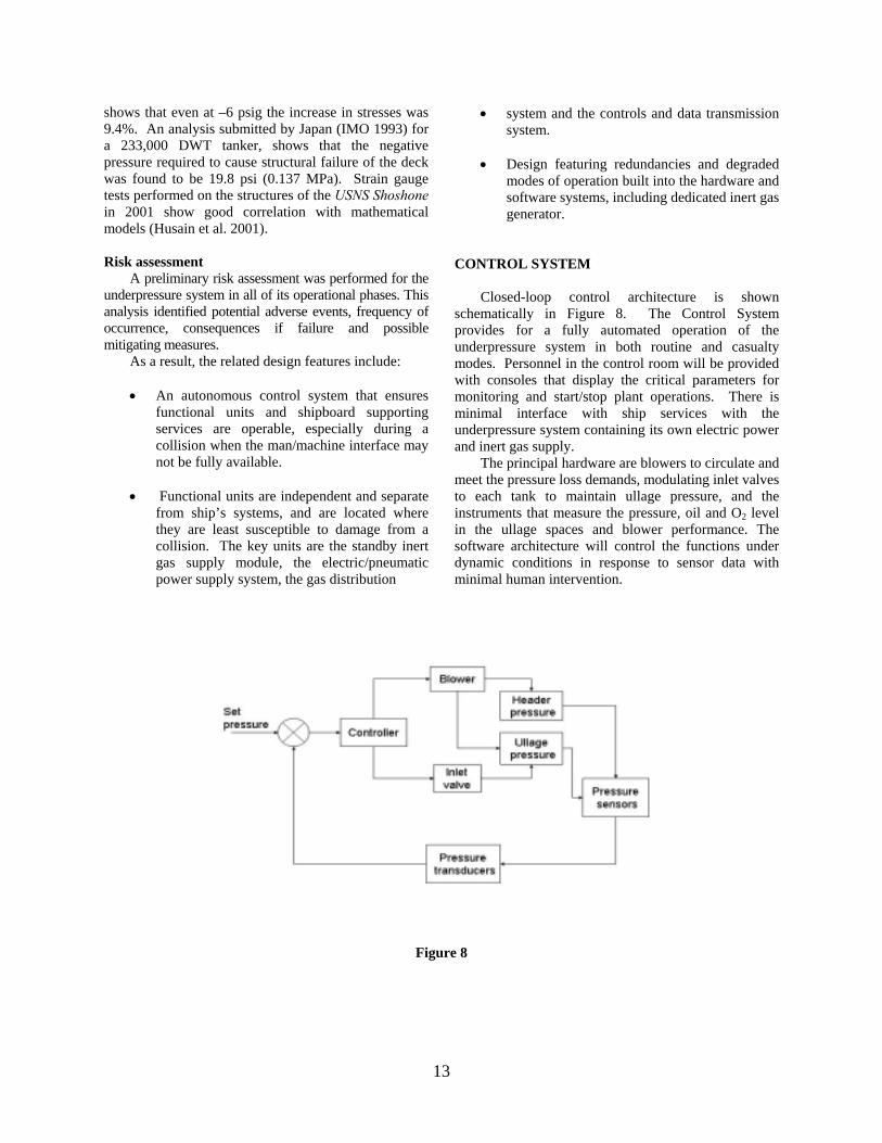
Closed-loop control architecture is shown

schematically in Figure 8. The Control System provides for a fully automated operation of the underpressure system in both routine and casualty modes. Personnel in the control room will be provided with consoles that display the critical parameters for monitoring and start/stop plant operations. There is minimal interface with ship services with the underpressure system containing its own electric power and inert gas supply.

The principal hardware are blowers to circulate and meet the pressure loss demands, modulating inlet valves to each tank to maintain ullage pressure, and the instruments that measure the pressure, oil and O2 level in the ullage spaces and blower performance. The software architecture will control the functions under dynamic conditions in response to sensor data with minimal human intervention.

Figure 8

13

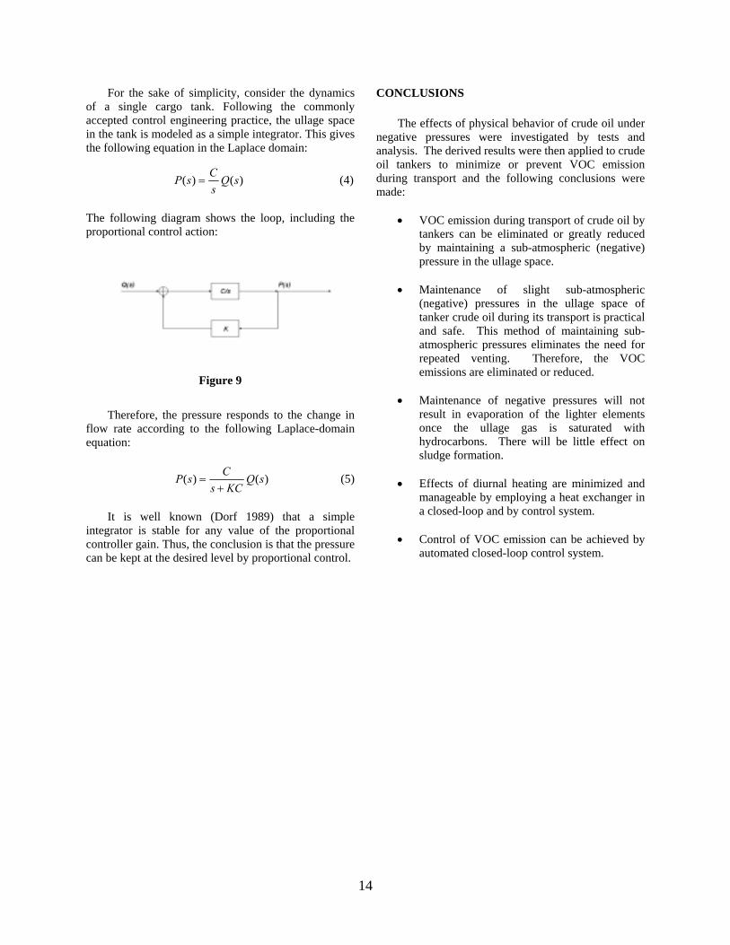
For the sake of simplicity, consider the dynamics of a single cargo tank. Following the commonly accepted control engineering practice, the ullage space in the tank is modeled as a simple integrator. This gives the following equation in the Laplace domain:

)()( sQsCsP = (4)

The following diagram shows the loop, including the proportional control action:

Figure 9

Therefore, the pressure responds to the change in

flow rate according to the following Laplace-domain equation:

)()( sQKCs

CsP+

=

(5)

It is well known (Dorf 1989) that a simple

integrator is stable for any value of the proportional controller gain. Thus, the conclusion is that the pressure can be kept at the desired level by proportional control.

CONCLUSIONS

The effects of physical behavior of crude oil under negative pressures were investigated by tests and analysis. The derived results were then applied to crude oil tankers to minimize or prevent VOC emission during transport and the following conclusions were made:

• VOC emission during transport of crude oil by

tankers can be eliminated or greatly reduced by maintaining a sub-atmospheric (negative) pressure in the ullage space.

• Maintenance of slight sub-atmospheric

(negative) pressures in the ullage space of tanker crude oil during its transport is practical and safe. This method of maintaining sub-atmospheric pressures eliminates the need for repeated venting. Therefore, the VOC emissions are eliminated or reduced.

• Maintenance of negative pressures will not

result in evaporation of the lighter elements once the ullage gas is saturated with hydrocarbons. There will be little effect on sludge formation.

• Effects of diurnal heating are minimized and

manageable by employing a heat exchanger in a closed-loop and by control system.

• Control of VOC emission can be achieved by

automated closed-loop control system.

14

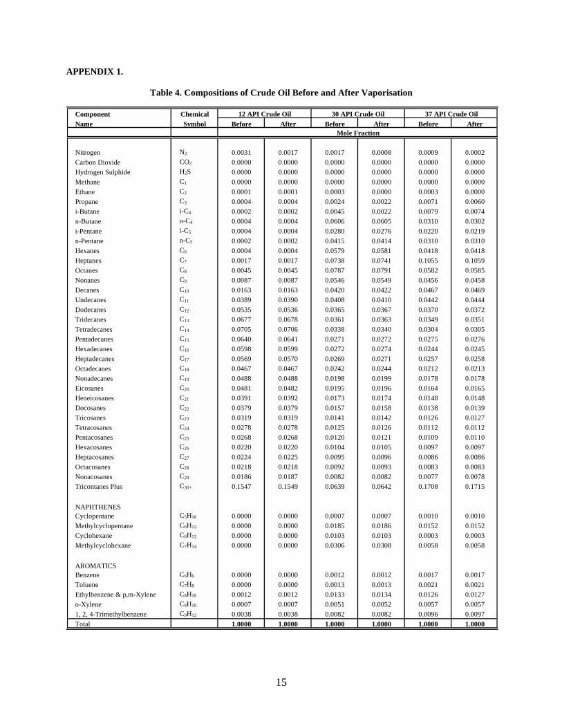
APPENDIX 1.

Table 4. Compositions of Crude Oil Before and After Vaporisation

Component Chemical 12 API Crude Oil 30 API Crude Oil 37 API Crude OilName Symbol Before After Before After Before After

Nitrogen N2 0.0031 0.0017 0.0017 0.0008 0.0009 0.0002Carbon Dioxide CO2 0.0000 0.0000 0.0000 0.0000 0.0000 0.0000Hydrogen Sulphide H2S 0.0000 0.0000 0.0000 0.0000 0.0000 0.0000Methane C1 0.0000 0.0000 0.0000 0.0000 0.0000 0.0000Ethane C2 0.0001 0.0001 0.0003 0.0000 0.0003 0.0000Propane C3 0.0004 0.0004 0.0024 0.0022 0.0071 0.0060i-Butane i-C4 0.0002 0.0002 0.0045 0.0022 0.0079 0.0074n-Butane n-C4 0.0004 0.0004 0.0606 0.0605 0.0310 0.0302i-Pentane i-C5 0.0004 0.0004 0.0280 0.0276 0.0220 0.0219n-Pentane n-C5 0.0002 0.0002 0.0415 0.0414 0.0310 0.0310Hexanes C6 0.0004 0.0004 0.0579 0.0581 0.0418 0.0418Heptanes C7 0.0017 0.0017 0.0738 0.0741 0.1055 0.1059Octanes C8 0.0045 0.0045 0.0787 0.0791 0.0582 0.0585Nonanes C9 0.0087 0.0087 0.0546 0.0549 0.0456 0.0458Decanes C10 0.0163 0.0163 0.0420 0.0422 0.0467 0.0469Undecanes C11 0.0389 0.0390 0.0408 0.0410 0.0442 0.0444Dodecanes C12 0.0535 0.0536 0.0365 0.0367 0.0370 0.0372Tridecanes C13 0.0677 0.0678 0.0361 0.0363 0.0349 0.0351Tetradecanes C14 0.0705 0.0706 0.0338 0.0340 0.0304 0.0305Pentadecanes C15 0.0640 0.0641 0.0271 0.0272 0.0275 0.0276Hexadecanes C16 0.0598 0.0599 0.0272 0.0274 0.0244 0.0245Heptadecanes C17 0.0569 0.0570 0.0269 0.0271 0.0257 0.0258Octadecanes C18 0.0467 0.0467 0.0242 0.0244 0.0212 0.0213Nonadecanes C19 0.0488 0.0488 0.0198 0.0199 0.0178 0.0178Eicosanes C20 0.0481 0.0482 0.0195 0.0196 0.0164 0.0165Heneicosanes C21 0.0391 0.0392 0.0173 0.0174 0.0148 0.0148Docosanes C22 0.0379 0.0379 0.0157 0.0158 0.0138 0.0139Tricosanes C23 0.0319 0.0319 0.0141 0.0142 0.0126 0.0127Tetracosanes C24 0.0278 0.0278 0.0125 0.0126 0.0112 0.0112Pentacosanes C25 0.0268 0.0268 0.0120 0.0121 0.0109 0.0110Hexacosanes C26 0.0220 0.0220 0.0104 0.0105 0.0097 0.0097Heptacosanes C27 0.0224 0.0225 0.0095 0.0096 0.0086 0.0086Octacosanes C28 0.0218 0.0218 0.0092 0.0093 0.0083 0.0083Nonacosanes C29 0.0186 0.0187 0.0082 0.0082 0.0077 0.0078Tricontanes Plus C30+ 0.1547 0.1549 0.0639 0.0642 0.1708 0.1715

NAPHTHENESCyclopentane C5H10 0.0000 0.0000 0.0007 0.0007 0.0010 0.0010Methylcyclopentane C6H12 0.0000 0.0000 0.0185 0.0186 0.0152 0.0152Cyclohexane C6H12 0.0000 0.0000 0.0103 0.0103 0.0003 0.0003Methylcyclohexane C7H14 0.0000 0.0000 0.0306 0.0308 0.0058 0.0058

AROMATICSBenzene C6H6 0.0000 0.0000 0.0012 0.0012 0.0017 0.0017Toluene C7H8 0.0000 0.0000 0.0013 0.0013 0.0021 0.0021Ethylbenzene & p,m-Xylene C8H10 0.0012 0.0012 0.0133 0.0134 0.0126 0.0127o-Xylene C8H10 0.0007 0.0007 0.0051 0.0052 0.0057 0.00571, 2, 4-Trimethylbenzene C9H12 0.0038 0.0038 0.0082 0.0082 0.0096 0.0097Total 1.0000 1.0000 1.0000 1.0000 1.0000 1.0000

Mole Fraction

15

APPENDIX 2. BACKGROUND FROM THERMODYNAMICS Phase Equilibrium

The thermodynamic behavior of a multicomponent mixture depends strongly on composition, pressure and temperature. At given reservoir temperature and different pressures, the components may be distributed between phases.

Phase and volumetric behavior of real reservoir system is most conveniently described by the respective phase diagrams, which are often called pressure-temperature diagrams.

The relationship between the temperature of a liquid and its vapor pressure for a pure substance is given by Clausius equation.

VTH

VVSS

dTdP

LV

LV

∆∆

=−−

=

It is an exact relationship between the slope of the saturated vapor pressure curve and two easily measured physical properties of the system, viz, the latent heat of vaporization (∆H) and the volume change on vaporization (∆V).

There is a commonly used approximation to this equation for vapor-liquid systems, due to Clausius, and so called the Clausius-Clapeyron equation. This makes three assumptions, which are generally reasonable for low-pressure systems for pure substances:

1. The latent heat of vaporization does not change over the temperature range being considered

2. The vapor is an ideal gas

3. Vapor volume is much larger than liquid volume

With those assumptions, the following approximate

equation can be derived for saturated vapor pressure:

TRHDP sat ∆

−=)ln(

The integration constant D, can be deduced from vapor pressure data at one temperature. This equation is similar in form to the empirically based Antoine equation; however, the Antoine equation has three empirical constants.

CTBAP sat

+−=)ln(

where

Psat is the vapor pressure T is the temperature in K The behavior of a mixture of multi-components is

not as simple as the behavior of a pure substance. Instead of a single line representing the vapor-pressure curve, there is a broad region in which two phases coexist. This region is called phase envelope. The phase envelope of multi-components systems can be predicted by equations of state. Cubic Equations of State Cubic equations of state are simple equations relating pressure, volume and temperature. Based on the first cubic equation of state that was proposed by van der Waals in 1873, an evolution of cubic EOS’ took place in focusing the interest on the application to petroleum engineering, as described above in the Path 1. The equations of state of this path may be written in the following generalized form:

.wbubVV

)T(abV

RTP 22 ++−

−= (6)

where P is the pressure, T the temperature, V the molar volume, R the gas constant and a and b are equation of state parameters which for a pure component are determined by imposing the critical conditions

.V

PVP

intPo.CritintPo.Crit02

2=

∂

∂=

∂∂

(7)

( ) ( )TaTa cα= (8)

c

cac P

TRa

22Ω= (9)

( )rT−+= 11 κα (10)

c

cb P

TRb Ω= (11)

The values of constants u, w, Ωa, Ωb, and κ are shown in Table 5.

16

Table 5 Cubic EOS u w Ωa Ωb κ

Van der Waals 0 0 0.421875 0.125000 Redlich-Kwong 1 0 0.427480 0.086640 Soave-Redlich-Kwong 1 0 0.427480 0.086640 0.480 + 1.574ω - 0.176ω2 Peng-Robinson 2 -1 0.457236 0.077796 0.37464+1.54226ω - 0.2699ω2 for ω ≤ 0.4

0.3796+1.485ω - 0.1644ω2 + 0.01667ω3 for ω > 0.4

Most of these modifications have been empirical and arbitrary, with parameters that are adjustable to fit certain kinds of experimental data such as vapor pressures, densities, or enthalpies.

In review, the PREOS and SRKEOS are the two most widely used cubic equations of state. The PREOS is comparable to SRK equation in simplicity and form. Peng and Robinson report that their equation predicts liquid densities better. They provide the same accuracy for VLE predictions and satisfactory volumetric predictions for vapor and liquid phases when used with volume translation.

The method of volume translation as proposed by Peneloux et al., modifies a two-constant cubic equation by introducing a third EOS constant c, but without changing the equilibrium calculations of the original, two-constant equation. The volume translation constant c eliminates the inherent volumetric deficiency suffered by all two constant equations. A simple correction term is applied to the EOS calculated molar volume:

cVV EOS −= (12)

where V is the corrected volume, VEOS is the calculated volume using EOS, and c is component specific constant.

In general, an equation of state is developed first for pure substances, and then extended to mixtures using mixing rules for combining the pure component parameters. The conflict between accuracy and simplicity is a big dilemma in developing an equation of state. Despite the wide use of high-speed computers, simplicity is still highly desired for easy and unequivocal applications of the equations to complex problems.

Mixing Rules for Cubic Equations of State

As discussed earlier in this section, the equations of state are generally developed for pure fluids first and then extended to mixtures. The mixture extension requires so-called mixing rules, which are simple means of calculating mixture parameters equivalent to those of pure substances. Most of the simple equations of state evolved from the van der Waals' equation use van der Waals' mixing rules with or without modifications.

Several authors have introduced in the mixing rules for the binary interaction coefficients kij, which are

empirically to be determined from the experimental vapour-liquid equilibrium data, for each binary present in the mixture. As pointed out by several authors, each kij factor can be considered independent of system temperature, pressure and composition. Some others have proved the strong dependence of kij from the temperature.

Heavy Fraction Characterization

The complete description of the performance of a petroleum reservoir is a complex calculation. Naturally occurring reservoir fluids typically consist of pure well-defined components including: CO2, N2, H2S, C1, C2, C3, i-C4, n-C4, i-C5, n-C5, C6,

and hundreds of heavy-end components (Heptanes and heavier, C7+). It is not possible to isolate all C7+ compounds or to assign accurate physical properties to each of them. Therefore, an approximate characterization of C7+ fractions using either experimental methods or mathematical methods has to be carried out. These methods include:

• Dividing C7+ fraction into a number of sub-fractions with known composition

• Defining the molecular weight, specific

gravity, and boiling point of each C7+ fraction.

• Estimation of critical properties, acentric factor and binary interaction coefficients according to the cubic EOS used.

There are some experimental methods for

quantifying the C7+ into discrete fractions. True boiling point (TBP) distillation provides the necessary data for a complete C7+ characterization, including specific gravity, molecular weight, and boiling point for each fraction, while gas chromatography (GC) analysis can only quantify the mass of C7+ fractions.

The choice of the characterization method certainly affects the outcome of reservoir fluid PVT prediction. However, the most reliable basis for C7+ characterization is the experimental data obtained by TBP distillation or chromatography.

17

Molecular Weight The molecular weight of the gas and liquid phase,

respectively, is given by

∑=i

iig MyM (13)

∑=i

iio MxM (14)

Density Phase density is given by

ZRTPM p

p =ρ (15)

Because the Z-factor is calculated as part of the EOS equilibrium solution, densities can be directly evaluated using the above formula. Component Properties and Correlations

A simple two-(or three) parameter equation of state requires the thermodynamic properties for each component in the mixture to be modeled. The critical pressure and critical temperature are needed. The acentric factor is also required. The binary interaction coefficients and volume translation parameters may be another input to the equation of state. This subset of input variables is used in the equation of state to predict thermodynamic properties of the mixture, such as saturation pressure, liquid volume in the two-phase region, composition of equilibrium phases, etc. Finally, when the phase density and viscosity are to be predicted by the equation of state the value of molecular weight, volume translation parameter, and the critical volume for each component has to be known.

The thermodynamic properties for the defined

reservoir hydrocarbons and non-hydrocarbons and injectants are taken from the literature. It includes Molecular weight MW, Critical Pressure Pc, Critical Temperature Tc, Critical Volume Vc, Acentric Factor ω, Boiling Temperature Tb and Specific Gravity γ.

For C7+ fractions the thermodynamic properties are found from empirical correlations in absence of experimental TBP data. Paraffin molecular weights are usually assumed when converting simulated distillation results to a mole-fraction basis. The best estimates of γ and Tb would come from a TBP analysis of a sample from the same field, and the next-best source would be the TBP data from a field producing from the same geological formation. APPENDIX 3. THERMAL LOAD ANALYSIS

In this section the thermal properties of the inert gas flow system used to control the pressure in the ullage space of the seaborne oil tanks are analyzed. In this system there are a number of modular oil tanks through which an inert gas is pumped at a regulated pressure. The primary heat load on this system is solar radiation.

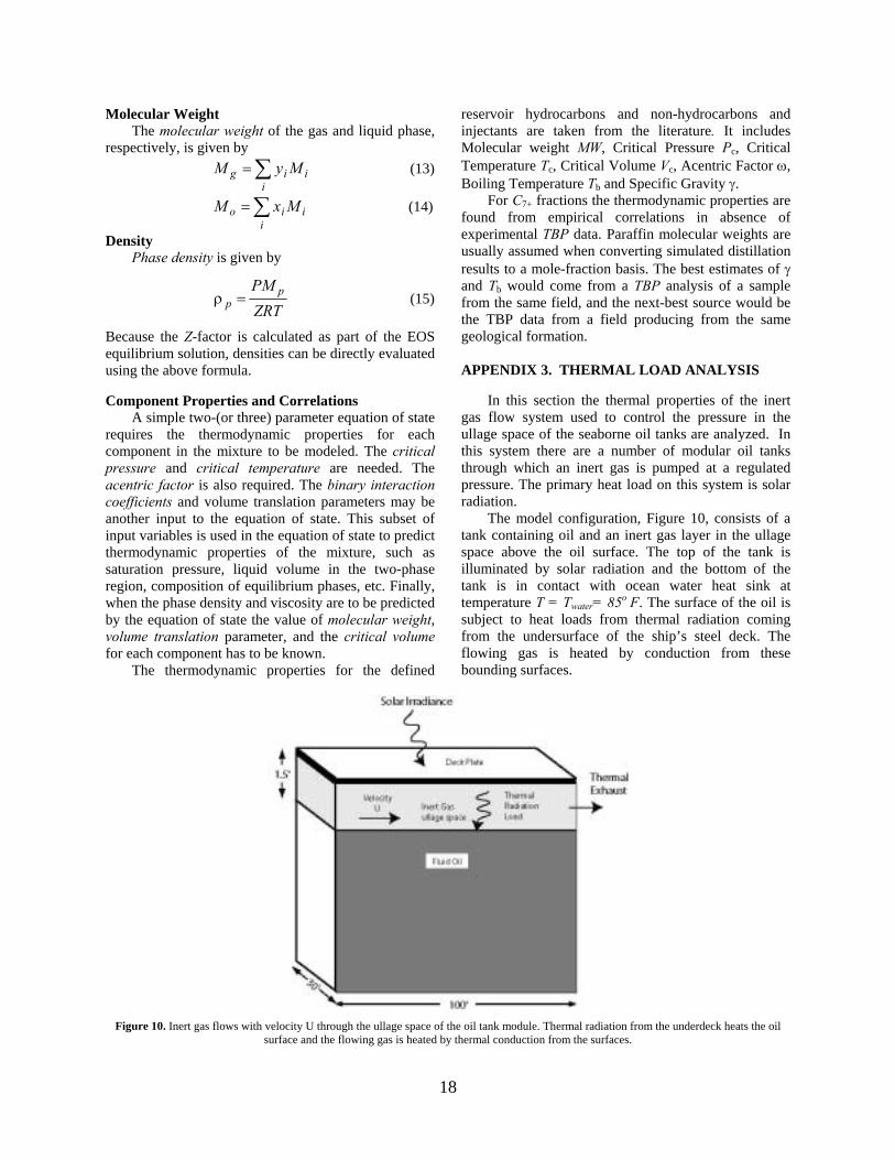
The model configuration, Figure 10, consists of a tank containing oil and an inert gas layer in the ullage space above the oil surface. The top of the tank is illuminated by solar radiation and the bottom of the tank is in contact with ocean water heat sink at temperature T = Twater= 85o F. The surface of the oil is subject to heat loads from thermal radiation coming from the undersurface of the ship’s steel deck. The flowing gas is heated by conduction from these bounding surfaces.

Figure 10. Inert gas flows with velocity U through the ullage space of the oil tank module. Thermal radiation from the underdeck heats the oil

surface and the flowing gas is heated by thermal conduction from the surfaces.

18

The dimensions of the oil tank are shown in Figure 10, Lx=30 ft, Ly = 100 ft and the depth of the gas layer is Lg=1.5 ft. The deck material is taken to be steel of Ld=1 inch thickness. The inert gas flows over the oil surface at mean velocity U.

Some of the characteristic time scales and heat loads can be estimated as follows. The thermal diffusion time constant of the steel deck is τ-deck = d2/αsteel ~ 1 minute, so the top and bottom surfaces of the steel deck are equilibrated on the timescales of interest. The thermal time constant of the oil mass is longer, τ-oil = (Loil/2)2αoil ~ (15ft)2/(3x10-3 ft2/hr) ~ 8.5 year. Hence, neglecting convection and mixing, the oil temperature distribution will not equilibrate during the voyage. Further, under conditions of surface heat load, the oil surface temperature can deviate from its initial temperature. The diurnal variations in heat load to the oil surface will change the temperature in a thin layer of oil δ ~sqrt(24hrs x αoil) ~ 3.3 in. Such heating can lead to increase evaporation of volatile hydrocarbons.

The heat load Qrad on the oil surface from radiative transfer depends on the difference between the deck temperature and the oil surface temperature and can be estimated as

( )oildeckdeckSB

rad TTT

Q −−+

=111 4

21

3

εε

σ

where ε1=0.95 and ε2 = 0.90 are the emissivities of the deck and oil surfaces respectively. These emissivity values may vary from these numbers in practice because of surface composition, roughness, and other factors. Taking Toil = 90 oF. and Tdeck = 165 oF. to approximate conditions of a summer day at noon, gives an estimate of Qrad ~ 60 BTU/ft2/hr. This heat flux will heat the oil surface significantly. In the following

calculations the bulk oil temperature below this surface layer is assumed to be Tbulk = 90 oF.

The other heat load on the oil surface is thermal conduction through the gas layer; this turns out to be much smaller than the typical radiative heat load. Estimating the conductive heat load to the oil surface as

)( oildeckgas

gasgc TT

LK

Q −=

where Kgas = 0.0262 W/m-K, 0.015 BTU/hr/ft/F and Tdeck is the deck temperature, and Toil is the oil surface temperature. Taking Tdeck = 165 oF. gives an estimate for the conducted heat flux of Qgc ~ 0.4 BTU/hr/ft2. Hence, the radiation heat load will be the dominant factor in heating of the oil surface layer.

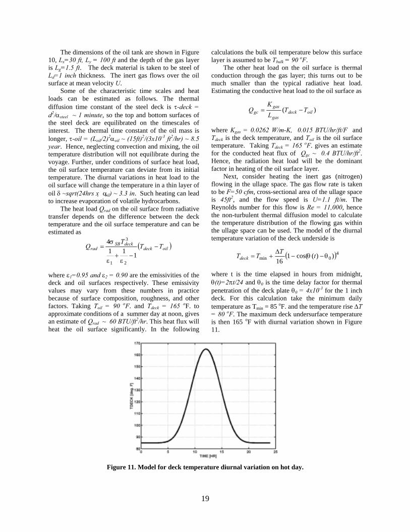
Next, consider heating the inert gas (nitrogen) flowing in the ullage space. The gas flow rate is taken to be F=50 cfm, cross-sectional area of the ullage space is 45ft2, and the flow speed is U=1.1 ft/m. The Reynolds number for this flow is Re = 11,000, hence the non-turbulent thermal diffusion model to calculate the temperature distribution of the flowing gas within the ullage space can be used. The model of the diurnal temperature variation of the deck underside is

( )40min ))(cos(1

16θθ −−

∆+= tTTTdeck

where t is the time elapsed in hours from midnight, θ(t)=2πt/24 and θ0 is the time delay factor for thermal penetration of the deck plate θ0 = 4x10-3 for the 1 inch deck. For this calculation take the minimum daily temperature as Tmin = 85 oF. and the temperature rise ∆T = 80 oF. The maximum deck undersurface temperature is then 165 oF with diurnal variation shown in Figure 11.

Figure 11. Model for deck temperature diurnal variation on hot day.

19

Since the gas transit time through the tank is much less than 24 hrs, the time dependence of deck temperature for this problem can be neglected. The gas temperature in the ullage spaces is modeled by the convection-diffusion equation.

0),(),( 2 =∇−∇⋅ yxTyxTv α

rr,

where v is the gas velocity and α is the gas thermal diffusivity. The boundary conditions are

=∂

∂=

==−

==

outlet Gas 0)100,(inlet Gas .85)0,(

.90),5.1(

.165),0(

xyT

FyT

FTxT

FTxT

o

ooil

odeck

The equation was solved numerically for the two

cases: low and high flow speed. The results showed that the gas thermal boundary layer expands to fill the ullage space at the outlet. The average gas temperature at the outlet is then Tout = (165 + 85)/2=125F. In case of 400 cfm flow the gas thermal boundary layer expands to approximately half the ullage space and the average temperature of the outlet gas is Tout = 105F. Finally, for flow rates in the range of 50 cfm, it can be concluded that the outlet average temperature of the gas will be

2)()(

)(tTtT

tT surfaceoildeckout

−+=

The time dependence indicates the diurnal

variation. The rate of heat transfer by the gas flow is then

−

+= − )(

2)()(

)( tTtTtT

Cmt inletsurfaceoildeck

p&Q

Header Heat Load

Finally, the heating of the gas manifold or header duct that carries the working gas to and from the oil tank array is addressed. The header assembly is located above deck consisting of cylindrical ducts having reflective paint surfaces. In the case without reflective paint, the duct wall temperature will be comparable to the deck temperature, having a maximum of Tw = Tdeck = 165 oF. Coating the duct with reflective aluminum paint having emissivity of ε = 0.26 can lower the duct temperature to the range of Tw = 123 oF. under

optimum conditions. Generally, the duct wall temperature and resulting gas stream are significantly affected by the surface coating. The header duct consists of a D=10inch diameter pipe of length L= 800ft, a flow rate of 1000cfm, and average flow velocity of U=30 ft/sec. The Reynolds number for the flow Re = UL/n = 1.5 x 105 is in the turbulent flow regime, hence the turbulent convective heat transport coefficient used.

NuD

kh gasturb

D =

The turbulent Nusselt number is evaluated using

the Petukhov equation (Pitts and Sissom 1998) with parameters for nitrogen gas as Nu = 298. The convective heat transfer coefficient is approximately hD = 5.4 BTU/hr ft2 oF

The gas temperature distribution along the header is then given by

x

w

xw eTTTT κ−=

−−

1,

where

pD

CmDh

&πκ =

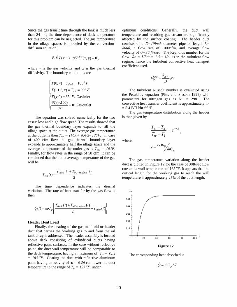
The gas temperature variation along the header

duct is plotted in Figure 12 for the case of 30ft/sec flow rate and a wall temperature of 165 oF. It appears that the critical length for the working gas to reach the wall temperature is approximately 25% of the duct length.

Figure 12 The corresponding heat absorbed is

TCmQ p ∆= &&

20

For the candidate tanker configuration the heat load generated by the header leg can be sizably reduced. For the same inlet temperature ( F) comparison is: °95

Unpainted wall = 65 x 103 BTU/hr

Painted wall = 29 x 103 BTU/hr

This is a consideration in the design. The conditions for the heat exchanger are based on a painted inlet header and a blower temp rise of F °20 Inlet Temp. to Heat Exchanger = 123 + 20 = 143 F ° Weight Flow = 1 LB/sec Outlet Temp. = 95 F ° Heat Exchanger Load = 82 x 103 BTU/hr

This is a relatively small heat-changer with a minimal pressure drop. REFERENCES: BIRD, R.B., STEWART, W.E, and LIGHTFOOT,

N.,Transport Phenomena, John Wiley & Sons, NY (2002).

CRABBE, D. and MCBRIDE, R., The World Energy Book, Nichols Publishing Co. NY (1978).

DORF, R.C., Modern Control Systems. 5th Ed., Addison-Wesley (1989).

GUNNER, T.J., CRUCOGSA - The Physical Behaviour of Crude Oil Influencing its Carriage by Sea, An INTERTANKO Publication (1999).GUNNER, T.J., “Physical Behavior of Crude Oil During Transportation and Its Impact on the Carriage of Crude Oil by Sea”. Marine Technology (2002) vol.39, No.4, pp.256-265.

HUSAIN, M., APPLE, R., THOMPSON, G., and SHARPE, R., “Full-Scale Test of the American Underpressure System (AUPS) on Board the USNS Shoshone.” SNAME Northern California Section Meeting. (Sept. 2001).

IMO (International Maritime Organization) Subcommittee On Ship Design And Equipment, 37th Session, Agenda Item 9.2 – DE 37/Inf .8 - 23rd December, 1993: “Alternative arrangements under Marpol 73/78 regulation I/13G - Ultimate Strength Analysis of Deck Structure of a crude oil tanker with an application of an Underpressure method.”

LIDE, D.R. and FREDERIKSE, H.P.R., Eds. CRC Handbook of Chemistry and Physics, CRC Press (1994).

MANSOUR, A.E. “Effect of Negative Pressure on Tanker Structure”. In: MH SYSTEMS. Concept Definition Documentation. Submitted to US Department of Transportation, Maritime Administration, Washington, D.C (1996).

PENG, D.Y. and ROBINSON, D.B.: ”A New Two Constant Equation of State”, Ind. Ing. Fund. (1976) 15, 59.

PITTS, D. and SISSOM, L., Theory and Problems of Heat Transfer, 2nd Ed., McGraw-Hill NY (1998).

REDLICH, O. and KWONG, J.N.S.: “On the Thermodynamic of Solutions - An Equation of State. Fugacities of Gaseous Solutions”, Chem. Reviews (1949) 44, 233.

SHTEPANI, E., WEINHARDT, B.E., and POTSCH, K.T.: “A New Modification of Cubic EOS Improves Prediction of Gas-Condensate Phase Behaviour”; 1996, SPE 36924, Europec ‘96, Milan, Italy, Vol. 2, p. 459 - 464.

SOAVE, G.: ”Equilibrium Constants from a Modified Redlich-Kwong Equation of State”, Chem. Eng. Sci. (1972) 27, 1197.

THOMAS, F.B., SHTEPANI, E., IMER, D., and BENNION, D.B.: “How Many Pseudo-Components Are Needed to Model Phase Behavior”, Journal of Canadian Petroleum Technology, (Jan. 2002), Vol. 41, No. 1, pp. 48-54.

WALAS, S.M.: Phase Equilibria in Chemical Engineering, Butterworth Publishers (1985), 3.

ZUCROW, M.J. and HOFFMAN, J.D., Gas Dynamics, V.1. John Wiley and Sons (1976).

21