CROSSING THE FINISH LINE - Princeton...
152
Appendix Material to Accompany CROSSING THE FINISH LINE COMPLETING COLLEGE AT AMERICA’S PUBLIC UNIVERSITIES William G. Bowen, Matthew M. Chingos, and Michael S. McPherson PRINCETON UNIVERSITY PRESS PRINCETON AND OXFORD Copyrighted Material Copyrighted Material Copyrighted Material
Transcript of CROSSING THE FINISH LINE - Princeton...

Appendix Material to Accompany
C R O S S I N G T H E F I N I S H L I N E
C O M P L E T I N G C O L L E G E A T A M E R I C A ’ S
P U B L I C U N I V E R S I T I E S
William G. Bowen, Matthew M. Chingos, and Michael S. McPherson
P R I N C E T O N U N I V E R S I T Y P R E S S P R I N C E T O N A N D O X F O R D
Copyrighted MaterialCopyrighted MaterialCopyrighted Material

Copyright © 2009 by Princeton University PressPublished by Princeton University Press, 41 William Street,
Princeton, New Jersey 08540
In the United Kingdom: Princeton University Press, 6 Oxford Street, Woodstock, Oxfordshire OX20 1TW
All Rights Reserved
This material has been composed in Adobe New Baskerville by Princeton Editorial Associates, Inc., Scottsdale, Arizona
press.princeton.edu
Copyrighted MaterialCopyrighted MaterialCopyrighted Material

Contents
Appendix B. Data Collection, Cleaning, and Imputation 5
Appendix C. High School Data (the National High School Database and the North Carolina High School Seniors Database) 27
Appendix D. Financial Aid Data 30
List of Appendix Tables 32
Appendix Tables 40
Copyrighted MaterialCopyrighted MaterialCopyrighted Material

THIS PAGE IS INTENTIONALLY BLANK
Copyrighted MaterialCopyrighted MaterialCopyrighted Material

A P P E N D I X B
Data Collection, Cleaning, and Imputation
THIS STUDY RELIES HEAVILY on two new databases created by research staffat The Andrew W. Mellon Foundation: (1) a “Flagships Database,” and(2) a “State Systems Database.” We describe each in this appendix. Wefirst describe the data collection process and the restrictions imposed tocreate as much uniformity across institutions as possible in the studentsincluded in our study (first-time, full-time freshmen and full-time trans-fer students of traditional college-going age). We then turn to the cre-ation of composite variables from multiple data sources and the imputa-tion of missing values of two key variables: family income quartile andhigh school GPA. Finally, we briefly discuss further restrictions imposedon the sample of students due to missing data.
The Flagships Database was assembled between September 2005 andAugust 2006. The core of the database is an institutional file that containsdetailed demographic, academic, and financial aid data on essentiallyevery student who entered one of 21 selective public universities in thefall of 1999 (although most universities excluded from their data studentswho began their studies on a part-time basis).1 The institutional file islinked with secondary data files provided by the College Board, ACT, theNational Student Clearinghouse, and the Higher Education Research In-stitute (HERI). Additionally, the home addresses of the students havebeen matched to their corresponding geographical codes (“geocodes”)and can be linked to census data down to the block level.
The State Systems Database, which covers a wider range of institutionsin four states—Maryland, North Carolina, Ohio, and Virginia—was assem-bled between June 2006 and June 2008. This database, also on the 1999entering cohort, includes institutional files from every public universityin Maryland, North Carolina, and Ohio as well as every public and private college and university in Virginia.2 Additionally, we have data onevery North Carolina student who was a high school senior in 1999. These
1. A handful of students were not included, such as those who explicitly for-bade the release of their educational records for research purposes (or any pur-pose), as well as, at one school, those who were not at least 18 years of age on thefirst day of classes in fall 1999.
2. The Ohio file includes only students at the main campuses of its public uni-versities; those at branch campuses are excluded.
Copyrighted MaterialCopyrighted MaterialCopyrighted Material
6 A P P E N D I X B
files are linked with secondary data files provided by the College Boardand the National Student Clearinghouse, and the students’ home ad-dresses have been linked to their corresponding geocodes.
As in the case of the College and Beyond Database, the Foundation’sconfidentiality agreements with the universities and secondary dataproviders mandate that these databases be maintained with “restricted ac-cess.” The next three sections focus on the Flagships Database, afterwhich we briefly return to the State Systems Database, which is similar inconstruction but different in scope.
THE SELECTION OF FLAGSHIP UNIVERSITIES AND DATA COLLECTION
The flagship universities in our study were selected from among themembership of the Association of American Universities (AAU), an or-ganization whose members are the leading research-intensive universitiesin the United States, both public and private. In August 2005, Nils Has-selmo, then president of the AAU, sent a message to the presidents andchancellors of the member universities informing them of the MellonFoundation’s proposed study of opportunity and the related data collec-tion effort. Shortly thereafter, William G. Bowen, then president of theFoundation, wrote to the presidents and chancellors of the 21 public uni-versities that were selected in an effort to obtain data from a representa-tive group based on factors such as geography, enrollment, graduationrates, and selectivity.3
Within a month of receipt of this invitation, 24 universities had agreedto participate. At their annual retreat in mid-September, the trustees ofthe Foundation strongly endorsed the new research agenda and proposeddata collection. Around the same time, a meeting of data contacts from ahandful of the participating universities was convened by the Foundationto discuss exactly which variables should be included in the data request.The final data request was submitted to the universities shortly thereafter.
Ultimately, three of the institutions declined to participate because ofstate laws, institutional mandates, or other policies that prohibited themfrom contributing the necessary data. Additionally, two of the invited par-
3. Of the 21 universities invited to participate, 5 had previously contributeddata to the College and Beyond Database. Pennsylvania State University con-tributed data on the 1951, 1976, 1989, and 1995 cohorts; the University of Michigan–Ann Arbor and the University of North Carolina–Chapel Hill con-tributed data on the 1951, 1976, and 1989 cohorts; and the University of Califor-nia–Los Angeles, the University of Illinois at Urbana-Champaign, and the Uni-versity of Virginia contributed data on the 1995 cohort.
Copyrighted MaterialCopyrighted MaterialCopyrighted Material
D A T A C O L L E C T I O N , C L E A N I N G , A N D I M P U T A T I O N 7
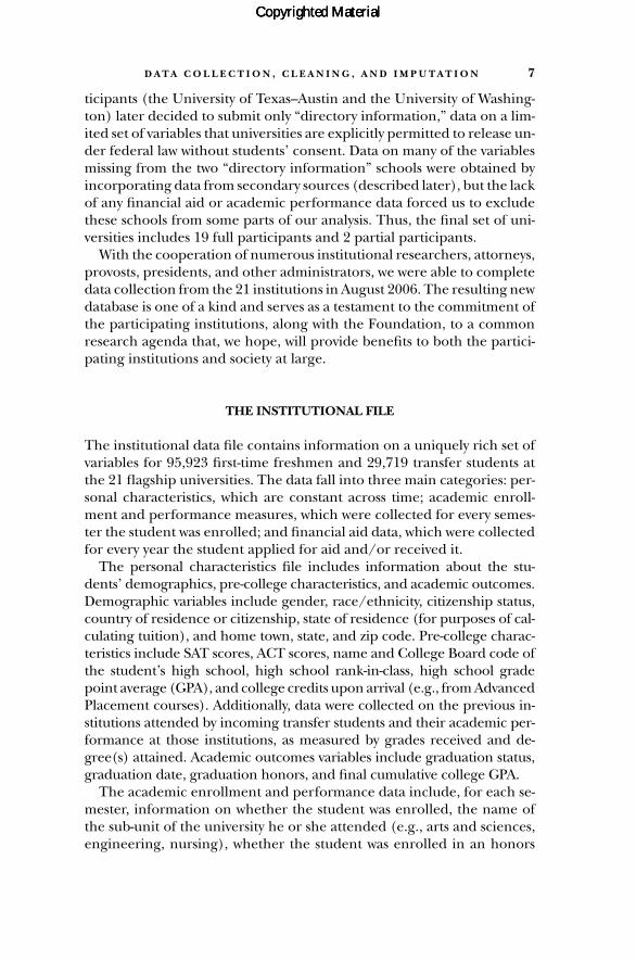
ticipants (the University of Texas–Austin and the University of Washing-ton) later decided to submit only “directory information,” data on a lim-ited set of variables that universities are explicitly permitted to release un-der federal law without students’ consent. Data on many of the variablesmissing from the two “directory information” schools were obtained byincorporating data from secondary sources (described later), but the lackof any financial aid or academic performance data forced us to excludethese schools from some parts of our analysis. Thus, the final set of uni-versities includes 19 full participants and 2 partial participants.
With the cooperation of numerous institutional researchers, attorneys,provosts, presidents, and other administrators, we were able to completedata collection from the 21 institutions in August 2006. The resulting newdatabase is one of a kind and serves as a testament to the commitment ofthe participating institutions, along with the Foundation, to a commonresearch agenda that, we hope, will provide benefits to both the partici-pating institutions and society at large.
THE INSTITUTIONAL FILE
The institutional data file contains information on a uniquely rich set ofvariables for 95,923 first-time freshmen and 29,719 transfer students atthe 21 flagship universities. The data fall into three main categories: per-sonal characteristics, which are constant across time; academic enroll-ment and performance measures, which were collected for every semes-ter the student was enrolled; and financial aid data, which were collectedfor every year the student applied for aid and/or received it.
The personal characteristics file includes information about the stu-dents’ demographics, pre-college characteristics, and academic outcomes.Demographic variables include gender, race/ethnicity, citizenship status,country of residence or citizenship, state of residence (for purposes of cal-culating tuition), and home town, state, and zip code. Pre-college charac-teristics include SAT scores, ACT scores, name and College Board code ofthe student’s high school, high school rank-in-class, high school gradepoint average (GPA), and college credits upon arrival (e.g., from AdvancedPlacement courses). Additionally, data were collected on the previous in-stitutions attended by incoming transfer students and their academic per-formance at those institutions, as measured by grades received and de-gree(s) attained. Academic outcomes variables include graduation status,graduation date, graduation honors, and final cumulative college GPA.
The academic enrollment and performance data include, for each se-mester, information on whether the student was enrolled, the name ofthe sub-unit of the university he or she attended (e.g., arts and sciences,engineering, nursing), whether the student was enrolled in an honors
Copyrighted MaterialCopyrighted MaterialCopyrighted Material

8 A P P E N D I X B
program or college, the name(s) and Classification of Instructional Pro-grams code(s) of the student’s major(s) and minor(s), the number ofcredit hours the student attempted (and his or her corresponding full-or part-time status), the number of credit hours the student successfullycompleted, and whether the student was living in a residence hall. A fewschools also were able to provide data on whether the student was study-ing abroad as well as, for students who did not live on campus, the zipcode of the student’s off-campus address.
The financial aid data include information from two main sources: thestudent’s and parents’ responses to the Free Application for Federal Stu-dent Aid (FAFSA) and the amounts of aid disbursed by source and type.The FAFSA responses are available only for students who applied for fi-nancial aid and include data on the student’s independent or dependentstatus, parents’ income and assets, student’s income and assets, expectedfamily contribution (EFC), student’s budget (cost of attendance), andstudent’s calculated need (budget minus EFC). Some schools also wereable to provide information on the student’s and parents’ marital statusand each parent’s educational attainment from the FAFSA form. Thedata on aid amounts are available primarily for students who applied foraid but also for some students who did not fill out the FAFSA but receivedpurely merit-based aid.4 In addition to information on the total amountof financial aid received, the following breakdowns are included: (1)grants and scholarships, loans, and work-study earnings; (2) need-basedand non-need-based aid;5 and (3) federal, state, institutional, and privateaid. Data were also collected on the amount of federal Pell Grants andSupplementary Educational Opportunity Grants the student received asa possible metric for comparisons across universities. Finally, data werecollected on whether the student paid resident (in-state) or non-resident(out-of-state) tuition each year.6
SECONDARY DATA SOURCES
The institutional file is linked to data from four secondary sources: theCollege Board, ACT, the National Student Clearinghouse, and the HERI.7
4. The FAFSA is primarily an application for need-based aid, although it is alsorequired for some non-need-based federal loan programs.
5. Only aid based purely on need is included in the need-based category; aidbased on a mix of merit and need is included in the non-need-based category.
6. Some schools reported the resident versus non-resident tuition data by semester.
7. The organizations that provided the secondary data matched the institu-tional records to their records using the student’s name, Social Security number,
Copyrighted MaterialCopyrighted MaterialCopyrighted Material

D A T A C O L L E C T I O N , C L E A N I N G , A N D I M P U T A T I O N 9
The College Board and ACT data provide vital demographic informationnot available from the institutions, such as self-reported family incomeand parental education.8 For the two universities that provided only di-rectory information (discussed earlier), we relied on the secondary datasources for essentially all of the demographic information, includingrace/ethnicity and gender. The College Board and ACT also provided ex-tensive survey responses about the students’ academic preparation inhigh school (e.g., courses taken, grades received, rank-in-class), extra-curricular activities in high school, educational aspirations, and plans forcollege (e.g., intended major, type of college most interested in).9 TheHERI file contains responses to a survey administered during the fresh-man year to students at six of the universities in our study.10 These surveydata include responses to a broad range of questions regarding the stu-dent’s first-year college experience.
The students’ home addresses at the time they took the SAT and/orthe ACT were matched to the corresponding geocodes so that studentscould be linked with the characteristics of the neighborhoods in whichthey lived during high school (and, in many cases, where they grew up).We are able to match students to census data down to the block level, al-though the variable of which we make the most use, median family in-come, is available beginning at only the block group level.
The Student Clearinghouse data allow us to track students who left theinstitution where they began their studies without graduating and en-rolled in another institution. The Clearinghouse file contains the nameand type (two- versus four-year and public versus private) of every insti-tution the student attended after August 1, 1999, as well as the dates of
and date of birth (the College Board and ACT also employed a small number ofother variables in their matching algorithm, such as high school attended andhome zip code). Not all schools provided Social Security numbers; the matchrates were lower, on average, for the schools that did not provide Social Securitynumbers than for those that did. All names and Social Security numbers werestripped from the database and destroyed after the matching was completed. Oneschool (Rutgers) made the matches on its own in cooperation with the CollegeBoard and the Clearinghouse (ACT data were not obtained, which was not par-ticularly problematic because most Rutgers students took the SAT) and providedde-identified data to Mellon.
8. Data on parental education are available only from the College Board;ACT does not collect this information.
9. The College Board survey, also called the Student Descriptive Question-naire, is filled out when students take the SAT. The ACT survey is filled out whenstudents register to take the test, which they must do at least three weeks prior totaking the test.
10. These six universities are Iowa State, Michigan, Ohio State, Stony Brook,UCLA, and UNC–Chapel Hill.
Copyrighted MaterialCopyrighted MaterialCopyrighted Material

10 A P P E N D I X B
each period for which he or she was enrolled. At the time we completedthe matches, the institutions that submitted enrollment data to the Clear-inghouse represented 91 percent of post-secondary enrollment in theUnited States. The Clearinghouse data also include information on de-grees received (name and type of institution granting the degree and de-gree title), but the coverage of the degree data is only about half that ofthe enrollment data.11
THE DATA FROM THE FOUR STATE SYSTEMS
The State Systems Database is structured in a fashion similar to the Flag-ships Database, with separate institutional and secondary data files foreach state. The Maryland file, which includes data maintained by the University System of Maryland as well as information submitted by the in-dividual institutions solely for this study, contains data on 10,565 fresh-men and 6,824 incoming transfer students at nine public universities.The availability of data on the variables that were not incorporated in thesystem data varies substantially across institutions.
The North Carolina university file, which is maintained by the Universityof North Carolina System, contains records for 27,465 freshmen and10,052 transfer students at 16 public universities. The North Carolina pre-college file, which is maintained by the North Carolina Education Re-search Data Center, contains records for 61,322 students who were highschool seniors in 1999, of which 17,389 are also among the incomingfreshmen in the university file. The pre-college file includes data on stu-dents’ high school, race/ethnicity, gender, and standardized test scores.12
The Ohio file, which is maintained by the Ohio Board of Regents, con-tains data on 35,726 freshmen and 12,288 transfers at the main campusesof 13 public universities (branch campuses are not included).
The Virginia file, which is maintained by the State Council of HigherEducation for Virginia, contains data on 34,195 freshmen and 13,043transfer students at 42 public and private colleges and universities. Sev-eral of these institutions had incomplete data or matriculated a smallnumber of students, so our analysis considers only a sub-set of the origi-
11. At the time we completed the matches, the institutions that submitted de-gree data to the Clearinghouse represented approximately half of postsecondaryenrollment in the United States.
12. Scores on tests administered to eighth-graders in reading and math as wellas on “end-of-course” exams administered to high school students in algebra, bi-ology, U.S. history, and English are available for a majority of students in thesedata.
Copyrighted MaterialCopyrighted MaterialCopyrighted Material

D A T A C O L L E C T I O N , C L E A N I N G , A N D I M P U T A T I O N 11
nal 42 institutions. (The next section of this appendix explains in detailwhich institutions were excluded and the effects of these exclusions onthe database.)
The institutional records from all four states include data on a total of107,951 freshmen and 42,207 transfer students (as well as the North Car-olina high school seniors) and contain information on variables similarto those included in the Flagships Database. The data from Maryland,North Carolina, and Virginia were matched to the databases maintainedby the College Board and the National Student Clearinghouse.13 Thematched records obtained from these organizations are identical in struc-ture to those described for the flagships. Staff of the Ohio Board of Re-gents provided us with the College Board and ACT records correspond-ing to the Ohio state system data (although Clearinghouse data were notavailable). However, these matched records were available only for Ohioresidents.
THE INITIAL RESTRICTION OF THE SAMPLE
Our main data set has been restricted to include only first-time, full-timefreshmen as well as full-time transfer students who first matriculated atone of the universities in our database in the fall of 1999. Some studentsactually started during the summer of 1999 but are included in our databecause their institution considers them part of the fall entering cohort.
Thus, students in the ’99 cohort who began their studies on a part-timebasis were excluded. We also excluded the small number of students whoappear in the demographic file but not in the enrollment file. These stu-dents either have erroneous records or dropped out so soon after en-rolling that they are not captured in the enrollment data.
We also imposed an age cut-off of 24 in order to try to restrict the sam-ple to traditional college-age (i.e., dependent) students. Students’ actualdependency status is available only for students who applied for financialaid, and we did not want to restrict our sample based on this limited in-formation. Although it is possible for students who are younger than 24to be independent (e.g., by being married or a veteran of the armed ser-vices), the number who fall into this category is probably small.
Finally, we excluded the small number of students who were neithercitizens nor permanent residents of the United States, because their socioeconomic status (SES) is difficult to measure and compare to thatof their classmates due to the varied countries in which they grew up.
13. Most college-bound students in these three states take the SAT, so we didnot match the institutional records to the ACT (as we did for the flagships).
Copyrighted MaterialCopyrighted MaterialCopyrighted Material

12 A P P E N D I X B
APPENDIX TABLE B.1Number of Freshmen and Transfer Students Dropped at Each Stage
of Sample Restriction and Reasons Dropped
Flagships State Systems (Total)
Reason Dropped Freshmen Transfers Freshmen Transfers
Not Observed in Enrollment Data 457 472 156 116Not Enrolled in Fall 1999 313 395 91 66Part-Time in Fall 1999 3,497 3,643 8,543 10,861Not a Citizen or Permanent
Resident of the United States 1,810 1,452 1,078 874Born before January 1, 1976 119 4,158 1,231 6,994Total Dropped 6,196 10,120 11,099 18,911
State Systems by State
Maryland North Carolina
Reason Dropped Freshmen Transfers Freshmen Transfers
Not Observed in Enrollment Data 29 84 35 10Not Enrolled in Fall 1999 43 64 0 0Part-Time in Fall 1999 193 1,245 2,897 2,196Not a Citizen or Permanent
Resident of the United States 75 151 238 192Born before January 1, 1976 77 1,030 251 2,096Total Dropped 417 2,574 3,421 4,494
Ohio Virginia
Reason Dropped Freshmen Transfers Freshmen Transfers
Not Observed in Enrollment Data 92 22 0 0Not Enrolled in Fall 1999 48 2 0 0Part-Time in Fall 1999 2,278 3,293 3,175 4,127Not a Citizen or Permanent
Resident of the United States 211 251 554 280Born before January 1, 1976 621 1,380 282 2,488Total Dropped 3,250 4,948 4,011 6,895
Source: Flagships Database and State Systems Database.Notes: The conditions are imposed in the order listed; the numbers would not be the same if the
order were changed (e.g., if students over age 24 were dropped before part-time students weredropped rather than after). Students in the Virginia state system are not dropped based on the firsttwo criteria due to the fact that several institutions did not report any enrollment data, and droppingbased on missing enrollment data would have caused them to be dropped from the analysis.
Copyrighted MaterialCopyrighted MaterialCopyrighted Material
D A T A C O L L E C T I O N , C L E A N I N G , A N D I M P U T A T I O N 13
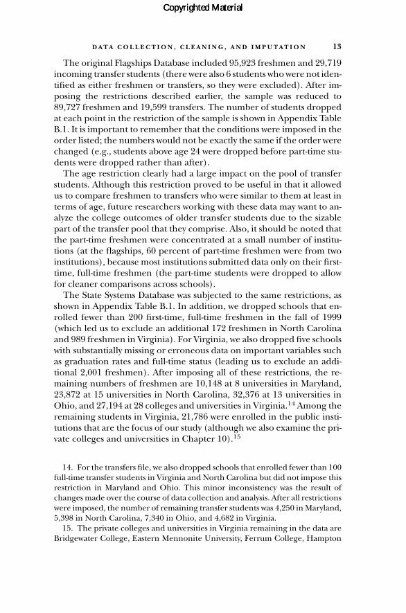
The original Flagships Database included 95,923 freshmen and 29,719incoming transfer students (there were also 6 students who were not iden-tified as either freshmen or transfers, so they were excluded). After im-posing the restrictions described earlier, the sample was reduced to89,727 freshmen and 19,599 transfers. The number of students droppedat each point in the restriction of the sample is shown in Appendix TableB.1. It is important to remember that the conditions were imposed in theorder listed; the numbers would not be exactly the same if the order werechanged (e.g., students above age 24 were dropped before part-time stu-dents were dropped rather than after).
The age restriction clearly had a large impact on the pool of transferstudents. Although this restriction proved to be useful in that it allowedus to compare freshmen to transfers who were similar to them at least interms of age, future researchers working with these data may want to an-alyze the college outcomes of older transfer students due to the sizablepart of the transfer pool that they comprise. Also, it should be noted thatthe part-time freshmen were concentrated at a small number of institu-tions (at the flagships, 60 percent of part-time freshmen were from twoinstitutions), because most institutions submitted data only on their first-time, full-time freshmen (the part-time students were dropped to allowfor cleaner comparisons across schools).
The State Systems Database was subjected to the same restrictions, asshown in Appendix Table B.1. In addition, we dropped schools that en-rolled fewer than 200 first-time, full-time freshmen in the fall of 1999(which led us to exclude an additional 172 freshmen in North Carolinaand 989 freshmen in Virginia). For Virginia, we also dropped five schoolswith substantially missing or erroneous data on important variables suchas graduation rates and full-time status (leading us to exclude an addi-tional 2,001 freshmen). After imposing all of these restrictions, the re-maining numbers of freshmen are 10,148 at 8 universities in Maryland,23,872 at 15 universities in North Carolina, 32,376 at 13 universities inOhio, and 27,194 at 28 colleges and universities in Virginia.14 Among theremaining students in Virginia, 21,786 were enrolled in the public insti-tutions that are the focus of our study (although we also examine the pri-vate colleges and universities in Chapter 10).15
14. For the transfers file, we also dropped schools that enrolled fewer than 100full-time transfer students in Virginia and North Carolina but did not impose thisrestriction in Maryland and Ohio. This minor inconsistency was the result ofchanges made over the course of data collection and analysis. After all restrictionswere imposed, the number of remaining transfer students was 4,250 in Maryland,5,398 in North Carolina, 7,340 in Ohio, and 4,682 in Virginia.
15. The private colleges and universities in Virginia remaining in the data areBridgewater College, Eastern Mennonite University, Ferrum College, Hampton
Copyrighted MaterialCopyrighted MaterialCopyrighted Material

14 A P P E N D I X B
CREATION OF COMPOSITE VARIABLES
In order to make the maximum use of our data, we created composite vari-ables when we had information on the same characteristic (e.g., race/ethnicity) from multiple sources. Variables were coded as follows (notethat, among the state systems, ACT data were collected only for Ohio):
• For race and gender, we first used data provided by the institution,then filled in missing values with data from the following sources(listed in the order in which we filled in the missing values): the SATquestionnaire, the ACT questionnaire, and the Advanced Placement(AP) questionnaire. In practice, the vast majority of values were fromthe institution, the SAT, or the ACT.
• For home state, we first used the students’ address when they tookthe SAT or ACT, then filled in missing values with the home state pro-vided by the institution.
• We calculated students’ state residency status using primarily dataprovided by their institutions on whether they paid resident or non-resident tuition in their first semester or year of college. Non-resident students who paid resident tuition under a tuition reci-procity agreement were coded as in-state students. Missing values ofthe state residency status variable were filled in based on whether thestudents’ home state matched the state in which their institution islocated.
• For test scores, we first used the students’ most recent SAT scores asprovided by the College Board. We then filled in missing values us-ing their most recent ACT scores as provided by the ACT (convertedto the SAT scale using concordance tables published by the CollegeBoard). We then filled in missing values using the SAT and ACTscores provided by the institutions. The coding was done in this wayto reflect our preference for the most recent scores (which is whatthe College Board and ACT provided us) rather than the highestscore on each section (which is what many institutions use, in keep-ing with their admissions policies).
• High school GPA was provided by many, but not all, institutions. Wefilled in missing values using the imputation procedure describedlater.
University, Hollins University, Lynchburg College, Mary Baldwin College, Mary-mount University, Roanoke College, Shenandoah University, the University ofRichmond, Virginia Wesleyan College, and Washington and Lee University. Thepublic universities in Virginia, the other state systems, and the flagships are alllisted in Tables 1.1 and 1.2.
Copyrighted MaterialCopyrighted MaterialCopyrighted Material

D A T A C O L L E C T I O N , C L E A N I N G , A N D I M P U T A T I O N 15
• We identified students’ high schools by their College Entrance Ex-amination Board codes, first using data provided by the institutionand then using data from the SAT, ACT, and AP databases.
• We calculated family income quartile using the students’ family in-come as reported on their FAFSA. Missing values were filled in usingthe imputation procedure described later.
• Parental education was available from only a small number of institu-tions, and we filled in missing values using data first from the HERIfreshmen survey and then from the SAT questionnaire (the ACT ques-tionnaire does not include questions about parental education). Be-cause several of the universities in our study are located in states wheremost students do not take the SAT, we excluded these universities fromall parts of our analysis that include data on parental education.16
THE IMPUTATION OF MISSING FAMILY INCOME DATA
Our database contains a rich set of measures of students’ SES, includingmeasures of family income, parental education, and the characteristics ofthe neighborhoods where the students lived when they were in highschool. Perhaps most central to the purposes of our study is the mea-surement of family income, which is important for college outcomes interms of both its short-run impact on a family’s ability to pay for collegeand its long-run effects on the student’s academic preparation, motiva-tion, and other factors correlated with success in college.
We were able to measure the family income of 92 percent of the first-time, full-time freshmen at the flagship universities by drawing on threesources of income data: the incomes that students’ families reportedwhen they filled out the FAFSA, the family incomes that students reportedon the survey that accompanies the SAT and the ACT, and the medianfamily income of the census block group where the students’ family livedat the time the student took the SAT or ACT (usually during the junioror senior year of high school).17 The FAFSA incomes are most likely to
16. The flagship universities without sufficient parental education data are theUniversity of Illinois at Urbana-Champaign, the University of Iowa, the Univer-sity of Minnesota–Twin Cities, the University of Nebraska–Lincoln, and the Uni-versity of Wisconsin–Madison. We also exclude the Ohio system from the parentaleducation analyses for the same reason. We are able to include Iowa State due tothe availability of data from the Higher Education Research Institute’s freshmansurvey.
17. Hereafter, the median family income of the student’s census block groupwill be referred to as “census income.” According to the U.S. Census Bureau,
Copyrighted MaterialCopyrighted MaterialCopyrighted Material
16 A P P E N D I X B
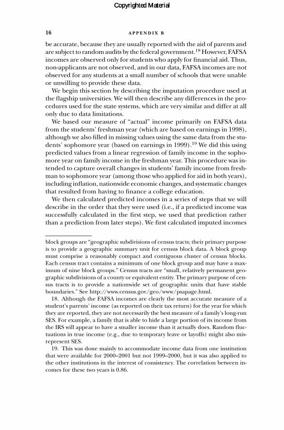
be accurate, because they are usually reported with the aid of parents andare subject to random audits by the federal government.18 However, FAFSAincomes are observed only for students who apply for financial aid. Thus,non-applicants are not observed, and in our data, FAFSA incomes are notobserved for any students at a small number of schools that were unableor unwilling to provide these data.
We begin this section by describing the imputation procedure used atthe flagship universities. We will then describe any differences in the pro-cedures used for the state systems, which are very similar and differ at allonly due to data limitations.
We based our measure of “actual” income primarily on FAFSA datafrom the students’ freshman year (which are based on earnings in 1998),although we also filled in missing values using the same data from the stu-dents’ sophomore year (based on earnings in 1999).19 We did this usingpredicted values from a linear regression of family income in the sopho-more year on family income in the freshman year. This procedure was in-tended to capture overall changes in students’ family income from fresh-man to sophomore year (among those who applied for aid in both years),including inflation, nationwide economic changes, and systematic changesthat resulted from having to finance a college education.
We then calculated predicted incomes in a series of steps that we willdescribe in the order that they were used (i.e., if a predicted income wassuccessfully calculated in the first step, we used that prediction ratherthan a prediction from later steps). We first calculated imputed incomes
block groups are “geographic subdivisions of census tracts; their primary purposeis to provide a geographic summary unit for census block data. A block groupmust comprise a reasonably compact and contiguous cluster of census blocks.Each census tract contains a minimum of one block group and may have a max-imum of nine block groups.” Census tracts are “small, relatively permanent geo-graphic subdivisions of a county or equivalent entity. The primary purpose of cen-sus tracts is to provide a nationwide set of geographic units that have stableboundaries.” See http://www.census.gov/geo/www/psapage.html.
18. Although the FAFSA incomes are clearly the most accurate measure of astudent’s parents’ income (as reported on their tax return) for the year for whichthey are reported, they are not necessarily the best measure of a family’s long-runSES. For example, a family that is able to hide a large portion of its income fromthe IRS will appear to have a smaller income than it actually does. Random fluc-tuations in true income (e.g., due to temporary leave or layoffs) might also mis-represent SES.
19. This was done mainly to accommodate income data from one institutionthat were available for 2000–2001 but not 1999–2000, but it was also applied tothe other institutions in the interest of consistency. The correlation between in-comes for these two years is 0.86.
Copyrighted MaterialCopyrighted MaterialCopyrighted Material

D A T A C O L L E C T I O N , C L E A N I N G , A N D I M P U T A T I O N 17
using data on the student’s expected family contribution, which is calcu-lated by the federal government based on the data provided on theFAFSA.20 Incomes were imputed as the predicted values from a linear regression of the natural logarithm of family income (as reported on theFAFSA) on the natural logarithm of EFC.21
We had real incomes for 55 percent of freshmen. The EFC imputationprocedure added another 6 percent of students. For the remainder of stu-dents we imputed income quartiles for those for whom we had self-reported data from the HERI, SAT, or ACT surveys. First we classified thestudents for whom we had actual incomes into income quartiles based onthe national distribution of family incomes of families with 16-year-oldchildren.22 We then ran an ordered probit regression of the actual in-come quartile on dummy variables corresponding to the responses to thesurvey question on family income as well the natural logarithm of the me-dian family income in the student’s census block group (recall that wematched students to the census block of the address where they residedwhen they took the SAT or ACT).23 The predicted values from an or-dered probit regression indicate the probability that the student falls intoeach of the quartiles. Their imputed quartile was selected as the quartilewith the maximum predicted probability. Imputed quartiles were filledin sequentially using the following combinations of predictor variables:
1. HERI self-reported income and the natural logarithm of census in-come
2. HERI self-reported income
20. This procedure was used only because there were three flagship universitiesthat provided data on EFC but not family income for a substantial number of theirfirst-year students. We applied it to all universities in the interest of consistency.
21. We used a log-log specification to improve fit. The correlation between theuntransformed income and EFC measures is 0.72, whereas for the logged mea-sured it is 0.77. In the prediction regression we dropped as outliers students withEFCs greater than $100,000.
22. The income quartiles are taken from the national income distribution offamilies with 16-year-old children in the IPUMS (Integrated Public Use MicrodataSeries) sample of 1 percent of the 2000 Census. The incomes for the quartileswere as follows: bottom quartile, less than $29,344 (in 1998 dollars); second quar-tile, $29,344–52,053; third quartile, $52,054–82,288; and top quartile, more than$82,288.
23. We chose an ordered probit model because it produced a better in-samplefit than did the other models we tried, including Heckman selection models andordinary least squares regressions. We also found that including a larger numberof predictors in the equation (such as additional characteristics of the neighbor-hood where the student grew up) did not improve the in-sample fit.
Copyrighted MaterialCopyrighted MaterialCopyrighted Material

18 A P P E N D I X B
3. SAT self-reported income and the natural logarithm of census income4. SAT self-reported income5. ACT self-reported income and the natural logarithm of census income6. ACT self-reported income
The survey questions we gave preference in this list were those that hada larger number of possible responses, each of which corresponded to asmaller range of incomes and thus made the question a better predictor ofincome quartile. We also ran equations without census income included inorder to be able to predict incomes for students for whom census incomedata were not available (e.g., their home address could not be matched toa census block group) but for whom self-reported incomes were avail-able.24 These students represented a minority of the sample, and we foundthat the prediction equation with census income excluded was almost asaccurate as the prediction equation with census income included.25
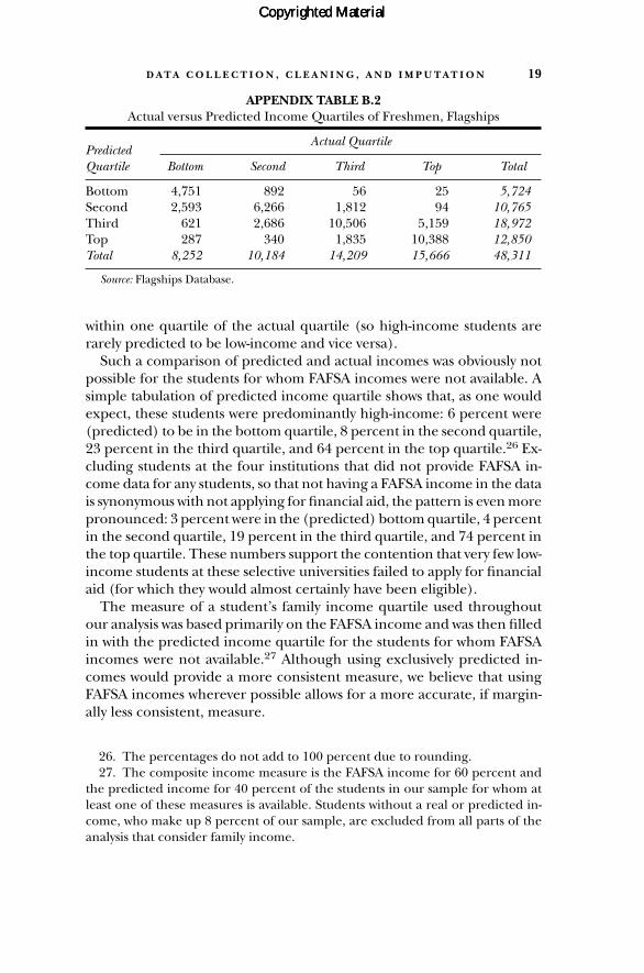
We generated predicted incomes for all students for whom self-reportedincome data were available, including both those with and without FAFSAincomes available. The predicted incomes of students for whom FAFSA in-comes were available allowed us to measure the accuracy of the in-samplepredictions. A cross-tabulation between FAFSA income quartile and pre-dicted income quartile (among the 48,311 students for whom we had bothmeasures) demonstrates the accuracy of the predictions for these students(Appendix Table B.2). If the prediction were perfect, all of the off-diagonal numbers on the table would be zero. Although this is not thecase, the prediction algorithm is generally quite accurate. For example,among students in the top income quartile, 66 percent were predicted tobe in the top quartile and another 33 percent were predicted to be in thethird quartile. Among those in the bottom quartile, 58 percent were pre-dicted to be in the bottom quartile and another 31 percent were predictedto be in the second quartile. In general, the predicted quartile is usually
24. Census data alone are not reliable in predicting FAFSA income, so we didnot predict incomes for students for whom census income data were available butself-reported income data were not.
25. The measure of self-reported income mapped fairly closely to that ofFAFSA income when quartiles were generated from both (i.e., students generallyhad a reasonably good sense of their parents’ income). Among students for whomFAFSA income data were not available (the ones for whom we relied on predictedincome data), we found that our measure of predicted income yielded higher in-comes on average than did the measure of raw self-reported income. This find-ing suggests that students tend to underreport their family incomes (of course wecannot say whether this is deliberate) and is consistent with the literature on thisissue (McPherson and Reischl, correspondence with Bowen et al., cited in Bowen,Kurzweil, and Tobin, p. 327).
Copyrighted MaterialCopyrighted MaterialCopyrighted Material
D A T A C O L L E C T I O N , C L E A N I N G , A N D I M P U T A T I O N 19
within one quartile of the actual quartile (so high-income students arerarely predicted to be low-income and vice versa).
Such a comparison of predicted and actual incomes was obviously notpossible for the students for whom FAFSA incomes were not available. Asimple tabulation of predicted income quartile shows that, as one wouldexpect, these students were predominantly high-income: 6 percent were(predicted) to be in the bottom quartile, 8 percent in the second quartile,23 percent in the third quartile, and 64 percent in the top quartile.26 Ex-cluding students at the four institutions that did not provide FAFSA in-come data for any students, so that not having a FAFSA income in the datais synonymous with not applying for financial aid, the pattern is even morepronounced: 3 percent were in the (predicted) bottom quartile, 4 percentin the second quartile, 19 percent in the third quartile, and 74 percent inthe top quartile. These numbers support the contention that very few low-income students at these selective universities failed to apply for financialaid (for which they would almost certainly have been eligible).
The measure of a student’s family income quartile used throughoutour analysis was based primarily on the FAFSA income and was then filledin with the predicted income quartile for the students for whom FAFSAincomes were not available.27 Although using exclusively predicted in-comes would provide a more consistent measure, we believe that usingFAFSA incomes wherever possible allows for a more accurate, if margin-ally less consistent, measure.
APPENDIX TABLE B.2Actual versus Predicted Income Quartiles of Freshmen, Flagships
Predicted Quartile Bottom Second Third Top Total
Bottom 4,751 892 56 25 5,724Second 2,593 6,266 1,812 94 10,765Third 621 2,686 10,506 5,159 18,972Top 287 340 1,835 10,388 12,850Total 8,252 10,184 14,209 15,666 48,311
Source: Flagships Database.
Actual Quartile
26. The percentages do not add to 100 percent due to rounding.27. The composite income measure is the FAFSA income for 60 percent and
the predicted income for 40 percent of the students in our sample for whom atleast one of these measures is available. Students without a real or predicted in-come, who make up 8 percent of our sample, are excluded from all parts of theanalysis that consider family income.
Copyrighted MaterialCopyrighted MaterialCopyrighted Material

20 A P P E N D I X B
We used the same procedure for transfer students (with the equationsrun separately from those for the freshmen), except that HERI surveydata were not used because the HERI survey is given only to freshmen.
For students in the Maryland state system, several versions of the esti-mating equation were all found to produce very noisy results that did notline up well with actual income quartiles (likely because of the smallernumber of students in the Maryland state system compared to those inthe flagships and the other state systems). Predicted income quartiles forboth freshmen and transfers in Maryland were taken directly from theSAT survey responses, which were matched as closely as possible to theincome quartile bands.
For students in the North Carolina state system, actual family incomeswere available only for financial aid applicants at the University of NorthCarolina–Chapel Hill, but EFCs were available for aid applicants at all in-stitutions. We estimated the relationship between family income quartileand EFC in an ordered probit regression of income quartile on EFC andits square using data from the Virginia state system, then used the esti-mated parameters to predict family income quartile using the EFCs in theNorth Carolina data. We repeated this procedure (using the Virginiadata) to estimate the relationship between income quartile and self-reported income on the SAT survey (both with and without using the nat-ural logarithm of census income as a predictor) in order to fill in re-maining missing values. We then repeated this procedure for the NorthCarolina transfers (using the Virginia transfers to estimate the parame-ters of the prediction equations).
The procedure used for freshmen and transfers in Ohio was identical tothat used for the flagships, except HERI and census income data were notavailable for any students in that state system. The procedure used in Vir-ginia was also similar to that used for the flagships, except EFC, HERI, andACT data were not used. Only self-reported incomes from the SAT surveyand census incomes were used to predict family income quartile in Vir-ginia. The cross-tabulations of actual and predicted income quartiles offreshmen at each of the four state systems are shown in Appendix TableB.3. It is difficult to draw any conclusions based on the numbers for Mary-land and North Carolina, where actual incomes were available only for fi-nancial aid applicants at the flagships. However, the numbers for Ohio andVirginia resemble those for the flagships in showing a reasonably good fit.
THE IMPUTATION OF MISSING HIGH SCHOOL GPA DATA
Another vitally important variable used throughout our study is highschool GPA, which we find to be an incredibly powerful predictor of out-
Copyrighted MaterialCopyrighted MaterialCopyrighted Material

D A T A C O L L E C T I O N , C L E A N I N G , A N D I M P U T A T I O N 21
APPENDIX TABLE B.3Actual versus Predicted Income Quartiles of Freshmen, State Systems
Maryland
PredictedQuartile Bottom Second Third Top Total
Bottom 429 129 18 14 590Second 167 359 111 26 663Third 64 391 272 116 843Top 29 156 170 190 545Total 689 1,035 571 346 2,641
North Carolina
Predicted Quartile Bottom Second Third Top Total
Bottom 100 11 6 1 118Second 54 119 37 2 212Third 32 91 228 47 398Top 15 19 72 219 325Total 201 240 343 269 1,053
Ohio
Predicted Quartile Bottom Second Third Top Total
Bottom 1,992 436 27 16 2,471Second 1,419 3,184 1,289 39 5,931Third 245 1,092 5,303 2,169 8,809Top 35 93 572 2,584 3,284Total 3,691 4,805 7,191 4,808 20,495
Virginia
Predicted Quartile Bottom Second Third Top Total
Bottom 1,288 497 75 22 1,882Second 452 1,529 639 98 2,718Third 220 872 2,525 842 4,459Top 87 211 793 3,538 4,629Total 2,047 3,109 4,032 4,500 13,688
Source: State Systems Database.Notes: Sample sizes are very small in Maryland and North Carolina because actual in-
comes are available only for financial aid applicants at the flagships in those states.
Actual Quartile
Actual Quartile
Actual Quartile
Actual Quartile
Copyrighted MaterialCopyrighted MaterialCopyrighted Material

22 A P P E N D I X B
comes in college (Chapter 6). Among the flagship universities, 12 pro-vided high school GPAs for more than 90 percent of their freshmen, 1provided it for about half of its entering class, and another 8 did not pro-vide this information. All told, we have actual high school GPAs for 51percent of the freshmen in our data set. Fortunately, we were able to im-pute high school GPAs for an additional 41 percent of the students usingself-reported information from the College Board and ACT surveys aswell as data on the number of AP exams taken. We first describe the im-putation procedure used for the freshmen at the flagships, then discussany differences in the procedures used to estimate high school GPA forthe transfers and the students in the state systems.
The SAT survey contained more detailed questions relating to stu-dents’ academic experiences in high school than did the ACT, so for students who took the SAT and filled out the survey we imputed highschool GPA as the predicted values from a linear regression of actual high school GPA on the following set of variables:
• A continuous variable indicating the number of AP exams taken bythe student, as computed from data provided by the College Board(the only non-self-reported measure used to impute high schoolGPA).28
• Dummy variables corresponding to the student’s self-reported cu-mulative high school GPA (A+, A, A–, B+, B, B–, C+, C, C–, D+, D, E,or F). Students who did not respond to this question were excludedfrom the imputation procedure.
• Dummy variables corresponding to the student’s self-reported highschool rank (highest tenth, second tenth, second fifth, middle fifth,fourth fifth, lowest fifth, or no response).
• Dummy variables corresponding to the student’s self-reported aver-age grade (excellent, good, fair, passing, failing, or no response) ineach of the following subjects: social sciences/history, natural sci-ences, mathematics, foreign and classical languages, English, and artsand music.
• Dummy variables corresponding to whether the student reportedtaking at least one AP, accelerated, or honors course in each of thesubjects just listed.
• Dummy variables corresponding to the number of years the studentreported taking courses (none, 0.5 year, 1 year, 2 years, 3 years, 4years, more than 4 years, or no response) in each of the subjects justlisted.
28. Data on AP exams taken were not available for one university (Rutgers), sothe imputation algorithm was run separately with all variables except the numberof AP exams.
Copyrighted MaterialCopyrighted MaterialCopyrighted Material

D A T A C O L L E C T I O N , C L E A N I N G , A N D I M P U T A T I O N 23
Among the 31,616 freshmen with both an actual high school GPA and apredicted high school GPA from the SAT data available, the correlationbetween the two measures was 0.79.
We next imputed high school GPAs as the predicted values from a lin-ear regression of actual high school GPAs on the number of AP examstaken and the following variables from the ACT survey:
• Dummy variables corresponding to the student’s self-reported over-all high school GPA (A– to A, B to B+, B– to B, C to B–, C– to C, D toC–, or D– to D).
• Dummy variables corresponding to the student’s best estimate of hisor her high school rank (top quarter, second quarter, third quarter,or fourth quarter).
• Dummy variables corresponding to the program of high schoolcourses taken by the student (business or commercial, vocational-occupational, college preparatory, or “other or general”).
• Dummy variables corresponding to the number of years of coursestaken by the student (none, 0.5 year, 1 year, 1.5 years, 2 years, 2.5years, 3 years, 3.5 years, or 4 years or more) in each of the followingsubjects: English, mathematics, social studies (history, civics, geogra-phy, economics), natural sciences (biology, chemistry, physics), Span-ish, German, French, another foreign language, business or com-mercial, and vocational-occupational.
• Dummy variables corresponding to whether the student reportedtaking at least one AP, accelerated, or honors course in each of thefollowing subjects: English, mathematics, social studies, natural sci-ences, and foreign language.
Among the 20,165 students with both an actual high school GPA and apredicted high school GPA (from the ACT data) available, the correla-tion between the two measures was 0.76. Combining the two measures(first using the SAT predictions, then the ACT predictions to fill in miss-ing values) yielded a correlation between actual and imputed high schoolGPA of 0.80 among the 41,371 students for whom both measures wereavailable.
For some students in the database we have an actual high school GPAbut could not predict a high school GPA (due to missing SAT and ACTsurvey data). Although we often use a measure of high school GPA thatis a combination of actual and predicted values, we sometimes use onlythe predicted values because they comprise the only measure that is con-sistent across universities. In order to increase the number of students forwhom we have a predicted high school GPA, we used the actual GPAs ateach university to create a “pseudo-predicted” high school GPA. This wascalculated as the predicted values from a linear regression of predicted
Copyrighted MaterialCopyrighted MaterialCopyrighted Material

24 A P P E N D I X B
high school GPA on actual high school GPA interacted with universitydummies (in order to reflect the fact that the different high school GPAscales at each university likely lead to different relationships between ac-tual and predicted high school GPA). As a result, both our “combined”(actual and predicted) and “adjusted” (predicted and pseudo-predicted)measures are available for the same number of students: 82,775 fresh-men, or about 92 percent of the sample.
We used the same procedure to impute missing high school GPAs ofthe transfer students at the flagships. We also used it for freshmen andtransfer students in Maryland and North Carolina and for freshmen inVirginia, with the exception that we used only SAT data. Actual highschool GPAs were not available for any transfers in Virginia, so the NorthCarolina transfers data were used to estimate the parameters of the pre-diction equation, which we then used to predict high school GPAs for theVirginia transfers.
The same imputation procedure that we used for the flagships was usedfor freshmen and transfers in Ohio using both SAT and ACT data, withthe exception that we used the parameters estimated from the equationusing the flagships data to impute the Ohio high school GPAs due to theabsence of any actual high school GPAs in the Ohio data. The Ohio pre-diction equation also included a continuous variable indicating the num-ber of specific subject areas (out of 35 total) in which the student re-ported taking at least one AP, accelerated, or honors course.29
The correlation coefficients between actual and predicted high schoolGPAs (not including the “pseudo-predicted” high school GPAs, becausethey are strongly correlated with actual high school GPAs by construc-tion) are shown in Appendix Table B.4. The correlations are all in the0.80–0.90 range with only one exception (0.73 for Maryland freshmen).
EXCLUSION OF CASES WITH MISSING DATA
The restricted sample described earlier (with missing values of family in-come quartile and high school GPA filled in using the imputation pro-cedures just described) forms the core data file analyzed in our study—although other data files, such as the North Carolina high school file, are
29. A version of this variable was also used to predict high school GPA at theflagships and in the other three state systems. However, a coding error (not dis-covered until the conclusion of the analysis) resulted in the miscalculation of thisvariable at the flagships and non-Ohio state systems. This led the variable to havea coefficient very close to zero in the prediction equations, and thus the resultsare essentially the same as if we had omitted it from the equations entirely.
Copyrighted MaterialCopyrighted MaterialCopyrighted Material

D A T A C O L L E C T I O N , C L E A N I N G , A N D I M P U T A T I O N 25
also used. Throughout the study we use various subsets of this file, eachof which drops students with missing values on variables used in a partic-ular part of the analysis.
The analysis of patterns of educational attainment presented in Chap-ters 3 and 4 excludes students with missing data on the variables of inter-est (SES, race/ethnicity, and gender) as well as the control variables (stateresidency status, SAT/ACT scores, and high school GPA). These restric-tions were made throughout (as opposed to just when absolutely neces-sary) so that the raw and regression-adjusted results are based on identi-cal sets of students and thus can be compared. For the flagships, droppingstudents with missing values of state residency status, race/ethnicity, gen-der, or SAT/ACT scores excluded 2,174 freshmen, 63 percent of whomwere at the two universities that provided only directory information (thusrequiring us to rely on SAT/ACT survey data for almost all of the key vari-ables, including race/ethnicity and gender). Dropping students with miss-ing high school GPAs excluded another 5,335 freshmen. Dropping stu-dents with missing data on family income quartile excluded an additional4,333 freshmen. Finally, dropping students with missing parental educa-tion (at the 16 flagships where information on this variable was widelyavailable) excluded 3,978 freshmen. (Keep in mind that these numbersapply only when the restrictions are imposed in this order.)
The file used for the flagships analysis in Chapters 3 and 4 includes73,907 out of the original 89,727 students, or about 82 percent. Missing
APPENDIX TABLE B.4Correlation Coefficients between Actual and Predicted High School GPAs,
Freshmen and Transfer Students
Freshmen Transfers
Flagships 0.80 0.8841,371 2,190
Maryland System 0.73 0.843,164 212
North Carolina System 0.86 0.8619,486 1,467
Ohio System — —0 0
Virginia System 0.89 —13,353 0
Source: Flagships Database and State Systems Database.Notes: Correlation coefficients are computed using data on students for whom both ac-
tual and predicted high school GPAs are available, the number of whom appears beneatheach coefficient.
Copyrighted MaterialCopyrighted MaterialCopyrighted Material

26 A P P E N D I X B
data were only slightly more common in the data for the four state sys-tems. Imposing the same restrictions as earlier reduced the number ofstudents from 88,282 to 68,700 (about 78 percent of the original data).30
Although we do not believe that the dropped students at the flagshipsand in the state systems are a random sample of all students, exploratoryanalyses gave us confidence that excluding them does not significantlybias our results.31
A sample similar to the one described earlier is used elsewhere in thestudy, because the key variables are similar throughout. However, the useof additional variables (such as high school characteristics in Chapter 5and financial aid data in Chapter 9) often requires us to exclude addi-tional students with missing data on these variables. In situations in whichwe focus on a smaller number of variables, such as in the analysis of thepredictive power of SAT/ACT scores and high school GPAs in Chapter 6,we include students with missing data on variables not needed for thatparticular analysis. Finally, we sometimes exclude entire institutions forwhich we do not have data on a key variable, such as college grades, as isthe case for the two flagships that were able to provide only directory in-formation. Such restrictions are noted in the main text or in notes.
30. Essentially none of the non-resident students in the Ohio system werematched to the SAT and ACT records, so we were not able to impute the highschool GPA or family income quartile for these students (and recall that we donot have any actual high school GPAs from Ohio). As a result, most of our analy-ses exclude these students.
31. For example, we calculated graduation rates by income quartile for all stu-dents for whom data on this variable are available and obtained results qualita-tively similar to those presented in Chapter 3, where we exclude students withmissing values on any of the control variables.
Copyrighted MaterialCopyrighted MaterialCopyrighted Material

A P P E N D I X C
High School Data(the National High School Database and
the North Carolina High School Senior Database)
IN THIS APPENDIX to Chapter 5, we first describe the National High SchoolDatabase that research staff at The Andrew W. Mellon Foundation as-sembled from various sources. We then describe the unusually rich datawe have for the 1999 graduating cohort of high school seniors in NorthCarolina and the definition of the high school level variable used inChapter 5.
DESCRIPTION OF THE NATIONAL HIGH SCHOOL DATABASE
We assembled data describing every high school in the United Statesfrom various sources. (A high school is defined as any school that listedits highest grade offered as 12th grade.) Data on the total enrollment, lo-cation, and racial composition of public schools are from the NationalCenter for Education Statistics (NCES) Common Core of Data Public Elementary/Secondary School Universe Survey Data for 1998–1999 (theyear that most of the first-time freshmen in our study were high schoolseniors). The same data on private schools are from the NCES PrivateSchool Universe Survey for 1999–2000. This year was chosen because theprivate school survey is conducted only every other year.
Data on the number of students at each high school who took the SAT,their average SAT score, and AP test-taking patterns were provided by theCollege Board. Similar data on ACT test-taking at each high school wereprovided by the ACT. (We calculate the percentage taking the SAT/ACTas the maximum of the percentage taking the SAT and the percentagetaking the ACT because we do not know which students took both.) Theaddress of each high school was matched to its corresponding censusblock group, which was in turn matched to the median family income inthat block group in 2000 U.S. Census data.
High schools in the Common Core of Data and Private School Uni-verse Survey are identified by an NCES code. Our Flagships Database andState Systems Database, as well as the College Board and ACT records,
Copyrighted MaterialCopyrighted MaterialCopyrighted Material

28 A P P E N D I X C
identify high schools by their College Entrance Examination Board(CEEB) code. The NCES and CEEB codes were linked using a crosswalkcreated by researchers at the Mellon Foundation for the purposes of thisstudy.1
Summaries of the characteristics of high schools attended by variousstudent populations are provided in Table 5.1.
NORTH CAROLINA HIGH SCHOOLS IN 1999
Thanks to the cooperation of the North Carolina Department of PublicInstruction, the University of North Carolina System, the North CarolinaEducation Research Data Center, and the keepers of a number of na-tional databases, it was possible to assemble a remarkable set of data describing the characteristics of more than 300 public high schools inNorth Carolina and the characteristics of the roughly 60,000 graduatingseniors in 1999. The College Board contributed data on national test-taking behavior—both SAT scores and AP grades—and on family back-ground characteristics such as family income and parental education forthose students who took the SAT. (We do not have comparable familybackground data for other high school seniors, who amount to roughlyhalf of the total high school population.) Data from the Common Coreof Data for all U.S. high schools were used to identify the location of theschools and to obtain information on a variety of school characteristics,including size, percentage of minority students, and student-teacher ra-tios. School addresses were then used to match individual schools to theneighborhoods in which they are located—and thus to obtain census dataon the average family income of the neighborhoods. Finally, records forindividual seniors were matched with records maintained by the NationalStudent Clearinghouse so that we could see if graduating seniors went onto college and, if so, to which college or university. Institutional recordsprovided by public four-year colleges and universities in North Carolinaallowed us to determine which matriculants graduated and how success-ful they were in college.
Appendix Table 5.10 contains descriptive data on the distribution of1999 seniors among high schools in North Carolina with varying charac-teristics. It can be compared with Table 5.1, which contains comparablenational data.
1. This crosswalk was built on previous versions of such a crosswalk providedto us by Edward Freeland and Jesse Rothstein at Princeton University as well asstaff at the College Board.
Copyrighted MaterialCopyrighted MaterialCopyrighted Material

H I G H S C H O O L D A T A 29
As explained in the text, we assigned each high school to one of threeacademic levels (I, II, III) on the basis of how they scored on a combina-tion of four measures: percentage of seniors taking the SAT, average SATscores of the students who took the SAT, “adjusted” SAT scores for all stu-dents,2 and number of Advanced Placement courses taken by students.We put schools in the Level I category if they scored well (in the top thirdof the distribution of high schools) on at least three out of the four mea-sures, in Level III if they were in the bottom third of the distribution onthree of the four measures, and in Level II if they did not meet the crite-ria for inclusion in either Level I or Level III.3 As implied by AppendixTable 5.10, this procedure placed 13,739 students in Level I schools,32,412 students in Level II, and 14,473 students in Level III.
There is one major complication. In North Carolina, families havesome opportunity to select the high school their children attend. Theyexercise this choice first by deciding where to live—in a district with ex-cellent high schools or elsewhere. Then, within school districts, we aretold that policies vary widely. In some districts, parents are given somechoice as to which public high school within the district their child willattend. In other districts, there is less or no choice. We cannot begin toplumb the depths of this set of complications. All we can do is note thedirection of bias in the results that we now report. Because there is somedegree of parental choice as to the high school attended, we assume thatthose parents most concerned about their children’s educational futurewill opt, in general and to the extent that they can, for their children togo to Level I schools. So whatever evidence we find suggesting that at-tendance at Level I schools has a positive effect on subsequent outcomesshould be understood as a “maximum” estimate, driven in part by the un-observable characteristics of the students attracted to the Level I schools.
2. “Adjusted” SAT scores are calculated by combining the actual SAT scores forthose students who took the SAT (roughly half of all seniors) and predicted SATscores for the other students based on Algebra I and English I examinations takenby students in their freshman or sophomore year of high school, which were avail-able for almost all students.
3. More precisely, Level I schools met the following criteria on at least three ofthe four measures: 57–80 percent of the students took the SAT, the average SATscore among those who took the test was in the 1005–1490 range, the predictedSAT score was in the 944–1490 range, and AP tests were taken in 18–30 courses.Level III schools met the following criteria on at least three of the four measures:fewer than 46.3 percent of the students took the SAT, the average SAT scoreamong those who took the test was below 955, the predicted SAT score was below887, and AP tests were taken in fewer than 12 courses. Level II schools are all thosethat did not meet the criteria for inclusion in either Level I or Level III.
Copyrighted MaterialCopyrighted MaterialCopyrighted Material
A P P E N D I X D
Financial Aid Data
THE DATA IN CHAPTER 8
IN THE MAIN, the data presented in Chapter 8 are taken directly from theTrends in College Pricing and Trends in Student Aid publications of the Col-lege Board, available online at www.collegeboard.com/trends. Both pub-lications use data from the College Board’s Annual Survey of Colleges, asurvey of 3,500 postsecondary institutions across the country. We supple-ment this information with data from the National Postsecondary Stu-dent Aid Study, a widely used federal source of student aid research. Bothsources are nationally representative.
THE DATA IN CHAPTER 9
The data used in Chapter 9 come exclusively from the Flagships Databaseand the State Systems Database used in the rest of this volume. However,we are restricted to a subset of institutions for which we have varying de-grees of detail regarding students’ financial aid information. In all analy-ses we also restrict our sample to in-state, dependent, non-transfer students.Throughout the chapter we keep flagships and state system selectivity clus-ter (SEL) A institutions separate from state system SEL B institutions.
Our broadest analyses use only data on students’ total grants (and, con-sequently, net price), which are available for 20 flagship and SEL A insti-tutions and for 15 SEL B institutions. Information on students’ total loansis available for the same flagship and SEL A institutions but not for theSEL B institutions. Instead, we use total federal loan data for the 8 SEL Binstitutions in Virginia and, due to inconsistencies, exclude the remain-ing 7 SEL B institutions. In practice, total federal loans (including bothstudent and parent loans) approximate the total loan figure because ofthe importance of federal loan programs in financing millions of stu-dents’ higher education; Figures 9.9a and 9.9b show this for our data.
Detailed financial aid data are available for some institutions, allowingus to perform more specific analyses. We have grant and loan data for 11flagships by source, distinguishing between federal, state, institutional,and private aid. For 7 of these flagships, we also have information on the
Copyrighted MaterialCopyrighted MaterialCopyrighted Material

F I N A N C I A L A I D D A T A 31
type of federal loan, whether subsidized Stafford loan, unsubsidizedStafford loan, or Parent Loan for Undergraduate Students.
For our analysis of net price and graduation, we use adjusted gradua-tion rates to control for student demographic and academic characteris-tics within each university. There are just two differences between theseadjusted graduation rates and those used in Chapter 10: these are esti-mated separately by income quartile and exclude independent students(as reported in the Free Application for Federal Student Aid; we there-fore assume that all independent students apply for aid).
Copyrighted MaterialCopyrighted MaterialCopyrighted Material

List of Appendix Tables
Chapter 1Appendix Table 1.1. Characteristics of 21 Flagship Universities by
Selectivity Cluster 40Appendix Table 1.2. Characteristics of Universities in Four State Systems
by Selectivity Cluster or HBCU Status 42
Chapter 3Appendix Table 3.1a. Six-Year Graduation Rates by Socioeconomic Status
and Selectivity Cluster, 1999 Entering Cohort, Flagships 45Appendix Table 3.1b. Six-Year Graduation Rates by Socioeconomic Status
and Selectivity Cluster, 1999 Entering Cohort, State Systems 45Appendix Table 3.2a. Six-Year Graduation Rates by Parental Education
and Selectivity Cluster, 1999 Entering Cohort, Flagships 46Appendix Table 3.2b. Six-Year Graduation Rates by Parental Education
and Selectivity Cluster, 1999 Entering Cohort, State Systems 47Appendix Table 3.3a. Six-Year Graduation Rates by Family Income and
Selectivity Cluster, 1999 Entering Cohort, Flagships 48Appendix Table 3.3b. Six-Year Graduation Rates by Family Income and
Selectivity Cluster, 1999 Entering Cohort, State Systems 49Appendix Table 3.4. Six-Year Graduation Rates by SES, Stepwise
Regressions, 1999 Entering Cohort, 16 Flagships and Three State Systems 50
Appendix Table 3.5. Six-Year Graduation Rates by Race/Ethnicity and Gender, Stepwise Regressions, 1999 Entering Cohort, 21 Flagships and Four State Systems 51
Appendix Table 3.6a. Six-Year Graduation Rates by Race/Ethnicity, Gender, and Selectivity Cluster, 1999 Entering Cohort, Flagships 52
Appendix Table 3.6b. Six-Year Graduation Rates by Race, Gender, andSelectivity Cluster, 1999 Entering Cohort, State Systems 53
Appendix Table 3.7a. Transfer Graduation Rates by Socioeconomic Status and Selectivity Cluster, 1999 Entering Cohort, 16 Flagships and Four State Systems (Percent) 54
Appendix Table 3.7b. Transfer Graduation Rates by Race, Gender, andSelectivity Cluster, 1999 Entering Cohort, 21 Flagships and Three StateSystems (Percent) 54
Appendix Table 3.8. Six-Year Graduation Rates by First-Year GPA and Selectivity Cluster, 1999 Entering Cohort, Flagships and State System SEL Bs 55
Copyrighted MaterialCopyrighted MaterialCopyrighted Material
L I S T O F A P P E N D I X T A B L E S 33
Appendix Table 3.9. Six-Year Graduation Rates by Family Income, 1999Entering Cohort, Flagships and State System SEL Bs 56
Appendix Table 3.10. Six-Year Graduation Rates by Race/Ethnicity and Gender, 1999 Entering Cohort, Flagships and State System SEL Bs 57
Chapter 4Appendix Table 4.1a. Adjusted Major at Graduation by Socioeconomic
Status, 1999 Entering Cohort, Flagships 58Appendix Table 4.1b. Adjusted Major at Graduation by Socioeconomic
Status and Selectivity Cluster, 1999 Entering Cohort, State Systems 59Appendix Table 4.2a. Adjusted Major at Graduation by Parental
Education, 1999 Entering Cohort, Flagships 60Appendix Table 4.2b. Adjusted Major at Graduation by Parental
Education and Selectivity Cluster, 1999 Entering Cohort, State Systems 61
Appendix Table 4.3a. Adjusted Major at Graduation by Family Income, 1999 Entering Cohort, Flagships 62
Appendix Table 4.3b. Adjusted Major at Graduation by Family Income and Selectivity Cluster, 1999 Entering Cohort, State Systems 63
Appendix Table 4.4a. Unadjusted Major at Graduation by Race/Ethnicity and Gender, 1999 Entering Cohort, Flagships 64
Appendix Table 4.4b. Adjusted Major at Graduation by Race/Ethnicity and Gender, 1999 Entering Cohort, Flagships 65
Appendix Table 4.5a. Unadjusted Major at Graduation by Race, Gender, and Selectivity Cluster, 1999 Entering Cohort, State Systems 66
Appendix Table 4.5b. Adjusted Major at Graduation by Race, Gender, and Selectivity Cluster, 1999 Entering Cohort, State Systems 67
Appendix Table 4.6a. Probability of Finishing on Time by Socioeconomic Status and Selectivity Cluster, 1999 Entering Cohort, Flagships, Unadjusted and Adjusted 69
Appendix Table 4.6b. Probability of Finishing on Time by Socioeconomic Status and Selectivity Cluster, 1999 Entering Cohort, State Systems,Unadjusted and Adjusted 69
Appendix Table 4.7a. Probability of Finishing on Time by Parental Education and Selectivity Cluster, 1999 Entering Cohort, Flagships,Unadjusted and Adjusted 70
Appendix Table 4.7b. Probability of Finishing on Time by Parental Education and Selectivity Cluster, 1999 Entering Cohort, State Systems, Unadjusted and Adjusted 71
Appendix Table 4.8a. Probability of Finishing on Time by Family Income and Selectivity Cluster, 1999 Entering Cohort, Flagships, Unadjusted and Adjusted 72
Copyrighted MaterialCopyrighted MaterialCopyrighted Material

34 L I S T O F A P P E N D I X T A B L E S
Appendix Table 4.8b. Probability of Finishing on Time by Family Income and Selectivity Cluster, 1999 Entering Cohort, State Systems, Unadjusted and Adjusted 73
Appendix Table 4.9a. Probability of Finishing on Time by Race/Ethnicity,Gender, and Selectivity Cluster, 1999 Entering Cohort, Flagships,Unadjusted and Adjusted 74
Appendix Table 4.9b. Probability of Finishing on Time by Race, Gender, and Selectivity Cluster, 1999 Entering Cohort, State Systems, Unadjusted and Adjusted 75
Appendix Table 4.10a. Rank-in-Class at Graduation by Socioeconomic Status and Selectivity Cluster, 1999 Entering Cohort, Flagships, Unadjusted and Adjusted 76
Appendix Table 4.10b. Rank-in-Class at Graduation by Socioeconomic Status and Selectivity Cluster, 1999 Entering Cohort, State Systems,Unadjusted and Adjusted 77
Appendix Table 4.11a. Rank-in-Class at Graduation by Parental Education and Selectivity Cluster, 1999 Entering Cohort, Flagships, Unadjusted and Adjusted 78
Appendix Table 4.11b. Rank-in-Class at Graduation by Parental Education and Selectivity Cluster, 1999 Entering Cohort, State Systems, Unadjusted and Adjusted 79
Appendix Table 4.12a. Rank-in-Class at Graduation by Family Income and Selectivity Cluster, 1999 Entering Cohort, Flagships, Unadjusted and Adjusted 80
Appendix Table 4.12b. Rank-in-Class at Graduation by Family Income andSelectivity Cluster, 1999 Entering Cohort, State Systems, Unadjusted and Adjusted 81
Appendix Table 4.13a. Rank-in-Class at Graduation by Race/Ethnicity, Gender, and Selectivity Cluster, 1999 Entering Cohort, Flagships,Unadjusted and Adjusted 82
Appendix Table 4.13b. Rank-in-Class at Graduation by Race, Gender, andSelectivity Cluster, 1999 Entering Cohort, State Systems, Unadjusted and Adjusted 83
Appendix Table 4.14a. Predicting Rank-in-Class at Graduation by Race/Ethnicity, Gender, and Selectivity Cluster, 1999 Entering Cohort, Flagships 84
Appendix Table 4.14b. Predicting Rank-in-Class at Graduation by Race, Gender, and Selectivity Cluster, 1999 Entering Cohort, State Systems 85
Appendix Table 4.15a. Summary Outcomes by Socioeconomic Status, 1999 Entering Cohort, Flagships and State System SEL As, Unadjusted and Adjusted 86
Appendix Table 4.15b. Summary Outcomes by Socioeconomic Status, 1999 Entering Cohort, State System SEL Bs, Unadjusted and Adjusted 87
Copyrighted MaterialCopyrighted MaterialCopyrighted Material

L I S T O F A P P E N D I X T A B L E S 35
Appendix Table 4.16a. Summary Outcomes by Race/Ethnicity and Gender, 1999 Entering Cohort, Flagships and State System SEL As,Unadjusted and Adjusted 88
Appendix Table 4.16b. Summary Outcomes by Race and Gender, 1999 Entering Cohort, State System SEL Bs, Unadjusted and Adjusted 89
Chapter 5Appendix Table 5.1. Six-Year Graduation Rates by Mean SAT/ACT Score
of High School, National Data 90Appendix Table 5.2. Six-Year Graduation Rates by High School Rank,
National Data 91Appendix Table 5.3. Four-Year College Attendance by Academic Level of
High School, North Carolina 92Appendix Table 5.4. Six-Year Graduation Rates by Academic Level of High
School, North Carolina 93Appendix Table 5.5. Six-Year Graduation Rates by Academic Level of
High School and within University-Reported High School GPA Ranges, North Carolina 94
Appendix Table 5.6. Undermatch Rates by Parental Education and Family Income, North Carolina 95
Appendix Table 5.7. Undermatch Rates by Academic Level of High School for All Students, North Carolina 96
Appendix Table 5.8. Graduation Rates by Undermatch Status, North Carolina 97
Appendix Table 5.9. College-Going Patterns of Students in the Top Quartile of the Eighth-Grade Test Score Distribution by Academic Level of High School, North Carolina (Percent) 98
Appendix Table 5.10. Summary Statistics, North Carolina High Schools 99
Chapter 6Appendix Table 6.1. Graduation Rates by SAT/ACT Scores and Adjusted
High School GPA, 1999 Entering Cohort, Flagships 100Appendix Table 6.2. Graduation Rates by SAT/ACT Scores and Adjusted
High School GPA, 1999 Entering Cohort, State Systems 101Appendix Table 6.3. Graduation Rates by SAT Scores, ACT Scores, and
Adjusted High School GPA, 1999 Entering Cohort 102Appendix Table 6.4. Graduation Rates by SAT/ACT Scores and High
School GPA, 1999 Entering Cohort, Flagship SEL Is 103Appendix Table 6.5. Graduation Rates by SAT/ACT Scores and High
School GPA, 1999 Entering Cohort, Flagship SEL IIs 104Appendix Table 6.6. Graduation Rates by SAT/ACT Scores and High
School GPA, 1999 Entering Cohort, Flagship SEL IIIs 105Appendix Table 6.7. Graduation Rates by SAT/ACT Scores and High
School GPA, 1999 Entering Cohort, State System SEL Bs 106
Copyrighted MaterialCopyrighted MaterialCopyrighted Material

36 L I S T O F A P P E N D I X T A B L E S
Appendix Table 6.8. Graduation Rates by SAT/ACT Score and High School GPA, 1999 Entering Cohort, State System HBCUs 107
Appendix Table 6.9a. Graduation Rates by SAT/ACT Score and Adjusted High School GPA, 1999 Entering Cohort, Flagships 108
Appendix Table 6.9b. Graduation Rates by SAT/ACT Scores and Adjusted High School GPA, 1999 Entering Cohort, State Systems 109
Appendix Table 6.9c. Six-Year Graduation Rates by SAT/ACT Scores and Actual or Adjusted High School GPA, 1999 Entering Cohort 110
Appendix Table 6.10. Six-Year Graduation Rates by University-Reported High School GPA and Level of High School, 1999 North Carolina High School Seniors 111
Appendix Table 6.11. Bachelor’s Degree Attainment by SAT and High School GPA, 1999 North Carolina High School Seniors 112
Appendix Table 6.12. Six-Year Graduation Rates by SAT/ACT Scores, Adjusted High School GPA, Race, and Gender, 1999 Entering Cohort 113
Appendix Table 6.13. Six-Year Graduation Rates by SAT/ACT Scores, Adjusted High School GPA, and Family Income Quartile, 1999 Entering Cohort 114
Appendix Table 6.14. Six-Year Graduation Rates by SAT/ACT Scores, Adjusted High School GPA, Race/Ethnicity, and Gender, 1999 Entering Cohort, Flagships 115
Appendix Table 6.15. SAT Scores and High School GPA by StudentCharacteristics, 1999 North Carolina High School Seniors 116
Appendix Table 6.16. Rank-in-Class at Exit by SAT/ACT Scores and Adjusted High School GPA, 1999 Entering Cohort, Flagships 117
Appendix Table 6.17. Rank-in-Class at Exit by SAT/ACT Scores and Adjusted High School GPA, 1999 Entering Cohort, State Systems 118
Appendix Table 6.18. Graduation Rates by SAT/ACT Scores, High School GPA, and Average of SAT II Scores, 1999 Entering Cohort 119
Appendix Table 6.19a. Six-Year Graduation Rates by SAT/ACT Scores, High School GPA, and Average of AP Test Scores, 1999 Entering Cohort 120
Appendix Table 6.19b. Four-Year Graduation Rates by SAT/ACT Scores, High School GPA, and Average of AP Test Scores, 1999 Entering Cohort 121
Chapter 7Appendix Table 7.1a. Transfer Admissions at Flagships and State System
SEL As 122Appendix Table 7.1b. Transfer Admissions at State System SEL Bs 123Appendix Table 7.2. Characteristics of Freshmen and Transfers, 1999
Entering Cohort 124
Copyrighted MaterialCopyrighted MaterialCopyrighted Material

L I S T O F A P P E N D I X T A B L E S 37
Appendix Table 7.3. Bachelor’s Degree Attainment Rates of Transfer Students (Relative to Freshmen), 1999 Entering Cohort 124
Appendix Table 7.4a. Six-Year Graduation Rates (Percent) and Numbers of Freshmen Enrollees and Transfer Students by Family Income, 1999 Entering Cohort 125
Appendix Table 7.4b. Six-Year Graduation Rates (Percent) and Numbers of Freshmen Enrollees and Transfer Students by High School GPA, 1999 Entering Cohort 125
Appendix Table 7.4c. Six-Year Graduation Rates (Percent) of FreshmenEnrollees and Transfer Students by SAT/ACT Scores, 1999 Entering Cohort 126
Appendix Table 7.5. Major at Graduation of Freshmen Enrollees and Transfer Students (Percentage of Students in Each Field), 1999 Entering Cohort 126
Appendix Table 7.6. Rank-in-Class at Graduation of Transfer Students (Relative to Freshmen), 1999 Entering Cohort 127
Appendix Table 7.7a. Average Rank-in-Class at Graduation of FreshmenEnrollees and Transfer Students by High School GPA, 1999 EnteringCohort 128
Appendix Table 7.7b. Average Rank-in-Class at Graduation of FreshmenEnrollees and Transfer Students by SAT/ACT Scores, 1999 Entering Cohort 128
Appendix Table 7.8. Academic Predictors of Transfers’ College Outcomes, 1999 Entering Cohort 129
Appendix Table 7.9. Comparison of Predictors for Freshmen Enrollees versus Transfers, 1999 Entering Cohort 130
Appendix Table 7.10. Outcomes and Characteristics of Freshmen Enrollees and Transfers at HBCUs, 1999 Entering Cohort 131
Appendix Table 7.11. Outcomes and Characteristics of Freshmen Enrollees and Transfer Students with High School GPAs below 3.0, 1999 EnteringCohort 131
Appendix Table 7.12. Educational Attainment of the Population Aged 25–34 by State, 2000 (Percentage in Each Category) 131
Chapter 8Appendix Table 8.1. Average Tuition and Fees (Constant 2008 Dollars)
and Percent Change, 1978–79 to 2008–09 133Appendix Table 8.2. Average Percent Change in Published and Net
Tuition (Constant 2008 Dollars), 1993–94 to 2008–09 134Appendix Table 8.3. Average Amount Borrowed (Constant 2008 Dollars)
from Federal and Private Sources (among Borrowers) by Family Income Quartile, 1992–93 to 2003–04 135
Copyrighted MaterialCopyrighted MaterialCopyrighted Material
38 L I S T O F A P P E N D I X T A B L E S
Appendix Table 8.4. Average Amount Borrowed (Constant 2008 Dollars) from Federal and Private Sources (among Borrowers) by Sector, 1992–93 to 2003–04 135
Chapter 9Appendix Table 9.1a. Average Financial Aid Packages (1999 Dollars)
by Race/Ethnicity and Family Income, 1999 Entering Cohort, Flagships and State System SEL As 136
Appendix Table 9.1b. Average Financial Aid Packages (1999 Dollars) byRace/Ethnicity and Family Income, 1999 Entering Cohort, State System SEL Bs 138
Appendix Table 9.2a. Changes in Financial Aid Packages (Constant 2002Dollars) among Full-Time, Dependent, In-State FAFSA-Filers (Grant Aid) by EFC, 1999 Entering Cohort 140
Appendix Table 9.2b. Changes in Financial Aid Packages (Constant 2002Dollars) among Full-Time, Dependent, In-State FAFSA-Filers (Loan Aid) by EFC, 1999 Entering Cohort 142
Appendix Table 9.2c. Changes in Family Income, Tuition, and EFC (Constant 2002 Dollars) among Full-Time, Dependent, In-State FAFSA-Filers, 1999 Entering Cohort 144
Appendix Table 9.3a. Regression of Four-Year Adjusted Graduation Rates on Net Price (1999 Dollars) among Freshmen at Flagship Universities by Family Income, 1999 Entering Cohort 145
Appendix Table 9.3b. Regression of Six-Year Adjusted Graduation Rates on Net Price (1999 Dollars) among Freshmen at Flagship Universities by Family Income, 1999 Entering Cohort 145
Chapter 10Appendix Table 10.1a. Regressions of Adjusted Six-Year Graduation Rates
on Institutional Characteristics, 1999 Entering Cohort 146Appendix Table 10.1b. Regressions of Adjusted Six-Year Graduation Rates
on Institutional Characteristics, 1999 Entering Cohort 147Appendix Table 10.1c. Graduation Rates by Living in a Residence Hall in
the First Semester, 1999 Entering Cohort 148Appendix Table 10.2. Graduation Rates, Public and Private Institutions,
Raw and Adjusted (Compared to Public SEL I Flagships), 1999 Entering Cohort (Publics) and 1995 Entering Cohort (Privates) 149
Appendix Table 10.3. Graduation Rates, Virginia Public and Private Institutions, Raw and Adjusted (Compared to SEL A Public Universities), 1999 Entering Cohort 149
Appendix Table 10.4. Six-Year Graduation Rates by Income and Starting at an Honors College, 1999 Entering Cohort 150
Copyrighted MaterialCopyrighted MaterialCopyrighted Material
L I S T O F A P P E N D I X T A B L E S 39
Appendix Table 10.5. Six-Year Graduation Rates by Income and Public versus Private Control, 1999 Entering Cohort (Publics) and 1995 Entering Cohort (Privates) 150
Chapter 11Appendix Table 11.1. Differences in Six-Year Graduation Rates for Black
Men by Selectivity Cluster (Compared to SEL I Flagships), 1999 Entering Cohort 151
Appendix Table 11.2. Differences in Six-Year Graduation Rates for Hispanics by Selectivity Cluster (Compared to SEL I Flagships), 1999 Entering Cohort 151
Appendix BAppendix Table B.1. Number of Freshmen and Transfer Students
Dropped at Each Stage of Sample Restriction and Reasons Dropped 20Appendix Table B.2. Actual versus Predicted Income Quartiles of
Freshmen, Flagships 27Appendix Table B.3. Actual versus Predicted Income Quartiles of
Freshmen, State Systems 29Appendix Table B.4. Correlation Coefficients between Actual and
Predicted High School GPAs, Freshmen and Transfer Students 33
Copyrighted MaterialCopyrighted MaterialCopyrighted Material

AP
PE
ND
IXT
AB
LE
1.1
Ch
arac
teri
stic
s of
21
Flag
ship
Un
iver
siti
es b
y Se
lect
ivit
y C
lust
er
Ave
rage
%%
%%
%%
Clu
ster
Uni
vers
itySi
zeSA
T/A
CT
Whi
teB
lack
His
pani
cA
sian
Out
-of-S
tate
Tran
sfer
s
SEL
IU
niv
ersi
ty o
f Cal
ifor
nia
–Ber
kele
y3,
619
1315
314
945
1031
Un
iver
sity
of C
alif
orn
ia–L
os A
nge
les
4,13
112
8534
413
405
35U
niv
ersi
ty o
f Mar
ylan
d–C
olle
ge P
ark
3,89
212
4064
145
1333
36U
niv
ersi
ty o
f Mic
hig
an5,
515
1240
687
414
2813
Un
iver
sity
of N
orth
Car
olin
a–3,
390
1245
8111
25
2117
Ch
apel
Hill
Un
iver
sity
of V
irgi
nia
2,92
213
1076
103
1030
16
SEL
II
Pen
nsy
lvan
ia S
tate
Un
iver
sity
5,06
112
0586
54
533
5R
utge
rs, T
he
Stat
e U
niv
ersi
ty o
f 5,
291
1180
569
921
1119
New
Jer
sey
Un
iver
sity
of F
lori
da3,
717
1265
7011
126
533
Un
iver
sity
of I
llin
ois
at U
rban
a-6,
466
1200
718
613
714
Ch
ampa
ign
Un
iver
sity
of T
exas
–Aus
tin
6,92
511
9564
414
184
22U
niv
ersi
ty o
f Was
hin
gton
4,62
211
6054
23
2615
30U
niv
ersi
ty o
f Wis
con
sin
–Mad
ison
5,21
512
2078
34
640
17
Copyrighted MaterialCopyrighted MaterialCopyrighted Material
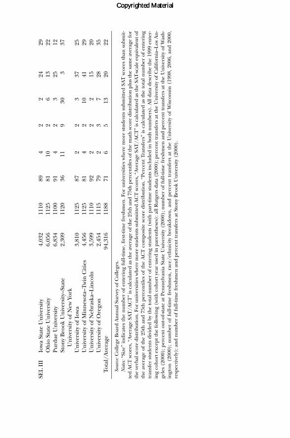
SEL
III
Iow
a St
ate
Un
iver
sity
4,03
211
1089
42
224
29O
hio
Sta
te U
niv
ersi
ty6,
056
1125
8110
26
1322
Purd
ue U
niv
ersi
ty6,
834
1100
914
23
2512
Ston
y B
rook
Un
iver
sity
–Sta
te
2,30
911
2036
119
303
37U
niv
ersi
ty o
f New
Yor
kU
niv
ersi
ty o
f Iow
a3,
810
1125
872
23
3725
Un
iver
sity
of M
inn
esot
a–Tw
in C
itie
s4,
456
1125
814
210
4129
Un
iver
sity
of N
ebra
ska–
Lin
coln
3,59
911
1092
22
215
20U
niv
ersi
ty o
f Ore
gon
2,45
411
1579
23
728
35To
tal/
Ave
rage
94,3
1611
8871
65
1320
22
Sour
ce:C
olle
ge B
oard
An
nua
l Sur
vey
of C
olle
ges.
Not
es:“
Size
” in
dica
tes
the
num
ber
of e
nte
rin
g fu
ll-ti
me,
firs
t-tim
e fr
esh
men
. For
un
iver
siti
es w
her
e m
ore
stud
ents
sub
mit
ted
SAT
sco
res
than
sub
mit
-te
d A
CT
sco
res,
“A
vera
ge S
AT
/AC
T”
is c
alcu
late
d as
the
aver
age
of th
e 25
th a
nd
75th
per
cen
tile
s of
the
mat
h s
core
dis
trib
utio
n p
lus
the
sam
e av
erag
e fo
rth
e ve
rbal
sco
re d
istr
ibut
ion
. For
un
iver
siti
es w
her
e m
ore
stud
ents
sub
mit
ted
AC
T s
core
s, “
Ave
rage
SA
T/A
CT
” is
cal
cula
ted
as th
e SA
T-sc
ale
equi
vale
nt o
fth
e av
erag
e of
th
e 25
th a
nd
75th
per
cen
tile
s of
th
e A
CT
com
posi
te s
core
dis
trib
utio
n. “
Perc
ent
Tran
sfer
s” is
cal
cula
ted
as t
he
tota
l num
ber
of e
nte
rin
gtr
ansf
er s
tude
nts
div
ided
by
the
tota
l num
ber
of e
nte
rin
g st
uden
ts (
wit
h p
art-t
ime
stud
ents
incl
uded
in b
oth
num
bers
). A
ll da
ta d
escr
ibe
the
1999
en
ter-
ing
coh
ort e
xcep
t th
e fo
llow
ing
(wit
h c
ohor
t yea
r us
ed in
par
enth
eses
): a
ll R
utge
rs d
ata
(200
0); p
erce
nt t
ran
sfer
s at
the
Un
iver
sity
of C
alif
orn
ia–L
os A
n-
gele
s (2
000)
; per
cen
t ou
t-of-s
tate
at
Pen
nsy
lvan
ia S
tate
Un
iver
sity
(20
00);
num
ber
of f
ull-t
ime
fres
hm
en a
nd
perc
ent
tran
sfer
s at
th
e U
niv
ersi
ty o
f W
ash
-in
gton
(20
00);
num
ber
of f
ull-t
ime
fres
hm
en,
race
/eth
nic
ity
brea
kdow
n,
and
perc
ent
tran
sfer
s at
th
e U
niv
ersi
ty o
f W
isco
nsi
n (
1998
, 20
06,
and
2000
,re
spec
tive
ly);
an
d n
umbe
r of
full-
tim
e fr
esh
men
an
d pe
rcen
t tra
nsf
ers
at S
ton
y B
rook
Un
iver
sity
(20
00).
Copyrighted MaterialCopyrighted MaterialCopyrighted Material
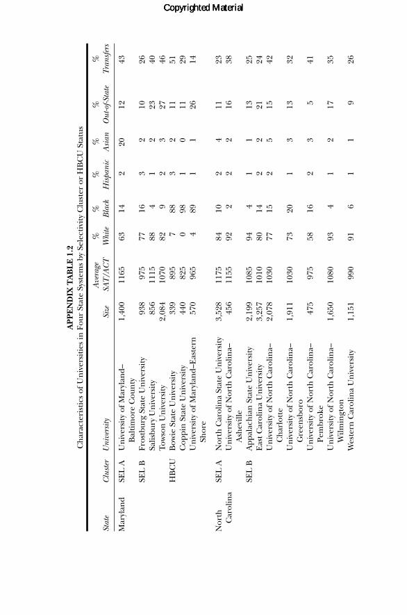
AP
PE
ND
IX T
AB
LE
1.2
Ch
arac
teri
stic
s of
Un
iver
siti
es in
Fou
r St
ate
Syst
ems
by S
elec
tivi
ty C
lust
er o
r H
BC
U S
tatu
s
Ave
rage
%%
%%
%%
Stat
eC
lust
erU
nive
rsity
Size
SAT
/AC
TW
hite
Bla
ckH
ispa
nic
Asi
anO
ut-o
f-Sta
teTr
ansf
ers
Mar
ylan
dSE
L A
Un
iver
sity
of M
aryl
and–
1,40
011
6563
142
2012
43B
alti
mor
e C
oun
tySE
L B
Fros
tbur
g St
ate
Un
iver
sity
938
975
7716
32
1026
Salis
bury
Un
iver
sity
856
1115
884
12
2340
Tow
son
Un
iver
sity
2,08
410
7082
92
327
46H
BC
UB
owie
Sta
te U
niv
ersi
ty33
989
57
883
211
51C
oppi
n S
tate
Un
iver
sity
440
825
098
10
1129
Un
iver
sity
of M
aryl
and–
Eas
tern
57
096
54
891
126
14Sh
ore
Nor
thSE
L A
Nor
th C
arol
ina
Stat
e U
niv
ersi
ty3,
528
1175
8410
24
1123
Car
olin
aU
niv
ersi
ty o
f Nor
th C
arol
ina–
456
1155
922
22
1638
Ash
evill
eSE
L B
App
alac
hia
n S
tate
Un
iver
sity
2,19
910
8594
41
113
25E
ast C
arol
ina
Un
iver
sity
3,25
710
1080
142
221
24U
niv
ersi
ty o
f Nor
th C
arol
ina–
2,07
810
3077
152
515
42C
har
lott
eU
niv
ersi
ty o
f Nor
th C
arol
ina–
1,91
110
3073
201
313
32G
reen
sbor
oU
niv
ersi
ty o
f Nor
th C
arol
ina–
475
975
5816
23
541
Pem
brok
eU
niv
ersi
ty o
f Nor
th C
arol
ina–
1,65
010
8093
41
217
35W
ilmin
gton
Wes
tern
Car
olin
a U
niv
ersi
ty1,
151
990
916
11
926
Copyrighted MaterialCopyrighted MaterialCopyrighted Material

HB
CU
Eliz
abet
h C
ity
Stat
e U
niv
ersi
ty40
280
518
811
048
20Fa
yett
evill
e St
ate
Un
iver
sity
799
860
789
21
1630
Nor
th C
arol
ina
A&
T U
niv
ersi
ty1,
538
905
296
00
2017
Nor
th C
arol
ina
Cen
tral
Un
iver
sity
624
865
297
00
1129
Win
ston
-Sal
em S
tate
Un
iver
sity
476
945
396
00
928
Oh
ioSE
L A
Mia
mi U
niv
ersi
ty3,
586
1180
894
22
278
SEL
BB
owlin
g G
reen
Sta
te U
niv
ersi
ty3,
516
1030
894
31
615
Cle
vela
nd
Stat
e U
niv
ersi
ty1,
049
910
6420
43
452
Ken
t Sta
te U
niv
ersi
ty3,
317
970
878
11
1021
Oh
io U
niv
ersi
ty3,
436
1090
953
11
1013
Shaw
nee
Sta
te U
niv
ersi
ty52
889
090
30
17
25U
niv
ersi
ty o
f Akr
on3,
002
970
8015
12
224
Un
iver
sity
of C
inci
nn
ati
3,71
010
5078
151
30
22U
niv
ersi
ty o
f Tol
edo
2,70
110
6076
153
23
25W
righ
t Sta
te U
niv
ersi
ty2,
132
1030
8612
11
229
Youn
gsto
wn
Sta
te U
niv
ersi
ty1,
933
970
848
21
920
HB
CU
Cen
tral
Sta
te U
niv
ersi
ty30
483
010
891
026
18
Vir
gin
iaSE
L A
Col
lege
of W
illia
m a
nd
Mar
y1,
299
1320
864
37
4410
Jam
es M
adis
on U
niv
ersi
ty3,
039
1170
904
25
2917
Un
iver
sity
of M
ary
Was
hin
gton
812
1205
913
33
3518
Vir
gin
ia T
ech
4,65
311
6588
42
628
15SE
L B
Ch
rist
oph
er N
ewpo
rt U
niv
ersi
ty69
310
3081
142
33
41G
eorg
e M
ason
Un
iver
sity
2,03
510
5566
87
1812
49L
ongw
ood
Un
iver
sity
818
1045
879
13
1021
Old
Dom
inio
n U
niv
ersi
ty1,
505
1025
6029
38
1145
(con
tinue
d)
Copyrighted MaterialCopyrighted MaterialCopyrighted Material
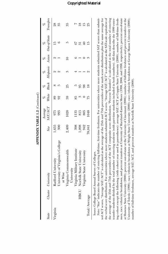
AP
PE
ND
IX T
AB
LE
1.2
(C
ontin
ued)
Ave
rage
%%
%%
%%
Stat
eC
lust
erU
nive
rsity
Size
SAT
/AC
TW
hite
Bla
ckH
ispa
nic
Asi
anO
ut-o
f-Sta
teTr
ansf
ers
Vir
gin
iaR
adfo
rd U
niv
ersi
ty1,
655
975
898
22
1528
Un
iver
sity
of V
irgi
nia
’s C
olle
ge30
099
592
52
16
35at
Wis
eV
irgi
nia
Com
mon
wea
lth
2,
409
1020
5925
310
535
Un
iver
sity
Vir
gin
ia M
ilita
ry I
nst
itut
e39
811
3585
54
647
7H
BC
UN
orfo
lk S
tate
Un
iver
sity
1,09
881
53
951
131
18V
irgi
nia
Sta
te U
niv
ersi
ty94
280
50
981
040
15To
tal/
Ave
rage
78,0
4110
4875
182
315
25
Sour
ce:C
olle
ge B
oard
An
nua
l Sur
vey
of C
olle
ges.
Not
es:“
Size
” in
dica
tes
the
num
ber
of e
nte
rin
g fu
ll-ti
me,
firs
t-tim
e fr
esh
men
. For
un
iver
siti
es w
her
e m
ore
stud
ents
sub
mit
ted
SAT
sco
res
than
sub
mit
-te
d A
CT
sco
res,
“A
vera
ge S
AT
/AC
T”
is c
alcu
late
d as
the
aver
age
of th
e 25
th a
nd
75th
per
cen
tile
s of
the
mat
h s
core
dis
trib
utio
n p
lus
the
sam
e av
erag
e fo
rth
e ve
rbal
sco
re d
istr
ibut
ion
. For
un
iver
siti
es w
her
e m
ore
stud
ents
sub
mit
ted
AC
T s
core
s, “
Ave
rage
SA
T/A
CT
” is
cal
cula
ted
as th
e SA
T-sc
ale
equi
vale
nt o
fth
e av
erag
e of
th
e 25
th a
nd
75th
per
cen
tile
s of
th
e A
CT
com
posi
te s
core
dis
trib
utio
n. “
Perc
ent
Tran
sfer
s” is
cal
cula
ted
as t
he
tota
l num
ber
of e
nte
rin
gtr
ansf
er s
tude
nts
div
ided
by
the
tota
l num
ber
of e
nte
rin
g st
uden
ts (
wit
h p
art-t
ime
stud
ents
incl
uded
in b
oth
num
bers
). A
ll da
ta d
escr
ibe
the
1999
en
ter-
ing
coh
ort
exce
pt t
he
follo
win
g (w
ith
coh
ort
year
use
d in
par
enth
eses
): a
vera
ge S
AT
/AC
T a
t C
oppi
n S
tate
Un
iver
sity
(20
00);
num
ber
of f
ull-t
ime
fres
h-
men
, rac
e/et
hn
icit
y br
eakd
own
, an
d pe
rcen
t tra
nsf
ers
at U
niv
ersi
ty o
f Mar
ylan
d–E
aste
rn S
hor
e (1
998,
200
6, a
nd
1998
, res
pect
ivel
y); p
erce
nt o
ut-o
f-sta
teat
Sh
awn
ee S
tate
Un
iver
sity
(20
00);
per
cen
t out
-of-s
tate
at t
he
Un
iver
sity
of C
inci
nn
ati (
2006
); n
umbe
r of
full-
tim
e fr
esh
men
an
d pe
rcen
t tra
nsf
ers
at th
eU
niv
ersi
ty o
f Tol
edo
(199
8); r
ace/
eth
nic
ity
brea
kdow
n a
t Wri
ght S
tate
Un
iver
sity
(20
00);
rac
e/et
hn
icit
y br
eakd
own
at G
eorg
e M
ason
Un
iver
sity
(20
00);
num
ber
of fu
ll-ti
me
fres
hm
en, a
vera
ge S
AT
/AC
T, a
nd
perc
ent t
ran
sfer
s at
Nor
folk
Sta
te U
niv
ersi
ty (
2000
).
Copyrighted MaterialCopyrighted MaterialCopyrighted Material

APPENDIX TABLE 3.1aSix-Year Graduation Rates by Socioeconomic Status and Selectivity Cluster,
1999 Entering Cohort, Flagships
SEL Is SEL IIs SEL IIIs
Unadjusted Middle SES 0.049 0.070 0.043[0.018]** [0.012]** [0.024]
High SES 0.103 0.145 0.135[0.021]** [0.015]** [0.029]**
Adjusted Middle SES 0.039 0.046 0.033[0.013]** [0.010]** [0.023]
High SES 0.086 0.117 0.119[0.014]** [0.013]** [0.029]**
Observations 20,077 17,755 15,699
Source: Flagships Database.Notes: Robust standard errors adjusted for clustering at the university level appear in
brackets. Coefficients indicate the predicted difference in graduation probability (from aprobit model) between the listed group and the reference group (low-SES students), hold-ing all control variables at their respective means. Adjusted differences control forSAT/ACT scores, high school GPA, state residency, race/ethnicity, gender, and universityattended.
* Significant at the .05 level.** Significant at the .01 level.
APPENDIX TABLE 3.1bSix-Year Graduation Rates by Socioeconomic Status and Selectivity Cluster,
1999 Entering Cohort, State Systems
Maryland North Carolina Virginia
SEL As SEL Bs SEL As SEL Bs SEL As SEL Bs
Unadjusted Middle SES 0.048 0.076 0.051 0.052 0.071 0.054[0.004]** [0.001]** [0.016]** [0.018]** [0.004]** [0.020]**
High SES 0.153 0.100 0.149 0.114 0.126 0.074[0.024]** [0.030]** [0.020]** [0.012]** [0.009]** [0.020]**
Adjusted Middle SES 0.029 0.087 0.035 0.070 0.066 0.067[0.011]** [0.012]** [0.014]* [0.010]** [0.007]** [0.021]**
High SES 0.110 0.117 0.112 0.145 0.110 0.105[0.007]** [0.006]** [0.017]** [0.011]** [0.008]** [0.021]**
Observations 4,039 2,855 6,371 9,750 9,696 6,416
Source: State Systems Database.Notes: Robust standard errors adjusted for clustering at the university level appear in brackets. Co-
efficients indicate the predicted difference in graduation probability (from a probit model) betweenthe listed group and the reference group (low-SES students), holding all control variables at their re-spective means. Adjusted differences control for SAT/ACT scores, high school GPA, state residency,race/ethnicity, gender, and university attended.
* Significant at the .05 level.** Significant at the .01 level.
Copyrighted MaterialCopyrighted MaterialCopyrighted Material
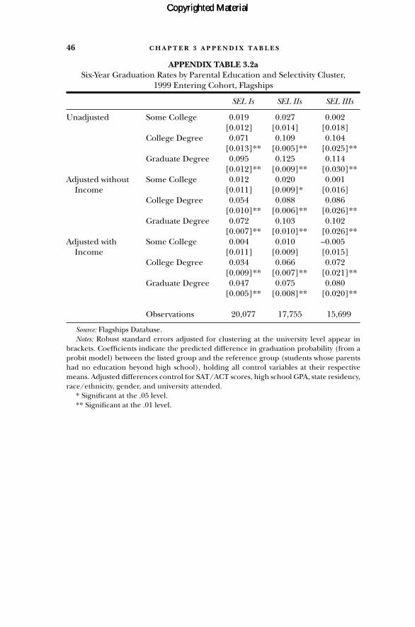
46 C H A P T E R 3 A P P E N D I X T A B L E S
APPENDIX TABLE 3.2aSix-Year Graduation Rates by Parental Education and Selectivity Cluster,
1999 Entering Cohort, Flagships
SEL Is SEL IIs SEL IIIs
Unadjusted Some College 0.019 0.027 0.002[0.012] [0.014] [0.018]
College Degree 0.071 0.109 0.104[0.013]** [0.005]** [0.025]**
Graduate Degree 0.095 0.125 0.114[0.012]** [0.009]** [0.030]**
Adjusted without Some College 0.012 0.020 0.001 Income [0.011] [0.009]* [0.016]
College Degree 0.054 0.088 0.086[0.010]** [0.006]** [0.026]**
Graduate Degree 0.072 0.103 0.102[0.007]** [0.010]** [0.026]**
Adjusted with Some College 0.004 0.010 –0.005Income [0.011] [0.009] [0.015]
College Degree 0.034 0.066 0.072[0.009]** [0.007]** [0.021]**
Graduate Degree 0.047 0.075 0.080[0.005]** [0.008]** [0.020]**
Observations 20,077 17,755 15,699
Source: Flagships Database.Notes: Robust standard errors adjusted for clustering at the university level appear in
brackets. Coefficients indicate the predicted difference in graduation probability (from aprobit model) between the listed group and the reference group (students whose parentshad no education beyond high school), holding all control variables at their respectivemeans. Adjusted differences control for SAT/ACT scores, high school GPA, state residency,race/ethnicity, gender, and university attended.
* Significant at the .05 level.** Significant at the .01 level.
Copyrighted MaterialCopyrighted MaterialCopyrighted Material

C H A P T E R 3 A P P E N D I X T A B L E S 47
APPENDIX TABLE 3.2bSix-Year Graduation Rates by Parental Education and Selectivity Cluster,
1999 Entering Cohort, State Systems
Maryland North Carolina Virginia
SEL As SEL Bs SEL As SEL Bs SEL As SEL Bs
Unadjusted Some College 0.049 0.016 –0.002 –0.011 –0.007 0.030[0.040] [0.035] [0.012] [0.009] [0.031] [0.024]
College Degree 0.131 0.075 0.074 0.067 0.060 0.073[0.027]** [0.024]** [0.002]** [0.012]** [0.016]** [0.016]**
Graduate Degree 0.153 0.090 0.121 0.098 0.081 0.063[0.038]** [0.031]** [0.019]** [0.017]** [0.022]** [0.011]**
Adjusted Some College 0.053 0.011 –0.027 0.005 –0.007 0.034without [0.047] [0.044] [0.016] [0.009] [0.031] [0.025]Income College Degree 0.112 0.073 0.039 0.087 0.052 0.090
[0.020]** [0.037]* [0.007]** [0.013]** [0.016]** [0.019]**Graduate Degree 0.120 0.098 0.064 0.116 0.060 0.086
[0.018]** [0.051] [0.015]** [0.013]** [0.016]** [0.012]**Adjusted Some College 0.045 0.006 –0.036 –0.001 –0.013 0.029
with [0.041] [0.045] [0.016]* [0.009] [0.029] [0.024]Income College Degree 0.092 0.062 0.015 0.070 0.033 0.077
[0.011]** [0.042] [0.008] [0.012]** [0.015]* [0.017]**Graduate Degree 0.096 0.084 0.030 0.091 0.035 0.069
[0.006]** [0.058] [0.015]* [0.014]** [0.016]* [0.012]**
Observations 4,039 2,855 6,371 9,750 9,696 6,416
Source: State Systems Database.Notes: Robust standard errors adjusted for clustering at the university level appear in brackets. Coefficients
indicate the predicted difference in graduation probability (from a probit model) between the listed groupand the reference group (students whose parents had no education beyond high school), holding all con-trol variables at their respective means. Adjusted differences control for SAT/ACT scores, high school GPA,state residency, race/ethnicity, gender, and university attended.
* Significant at the .05 level.** Significant at the .01 level.
Copyrighted MaterialCopyrighted MaterialCopyrighted Material

48 C H A P T E R 3 A P P E N D I X T A B L E S
APPENDIX TABLE 3.3aSix-Year Graduation Rates by Family Income and Selectivity Cluster,
1999 Entering Cohort, Flagships
16 Universities with Parental All 21 Universities Education Data
SEL Is SEL IIs SEL IIIs SEL Is SEL IIs SEL IIIs
Unadjusted Second Quartile 0.012 0.060 0.027 0.012 0.057 0.011[0.023] [0.013]** [0.018] [0.023] [0.022]** [0.022]
Third Quartile 0.049 0.095 0.065 0.049 0.103 0.057[0.030] [0.012]** [0.020]** [0.030] [0.017]** [0.018]**
Top Quartile 0.087 0.139 0.117 0.087 0.134 0.101[0.025]** [0.011]** [0.025]** [0.025]** [0.019]** [0.029]**
Adjusted Second Quartile 0.016 0.029 0.010 0.016 0.025 –0.003without [0.013] [0.013]* [0.018] [0.013] [0.017] [0.024]Parental Third Quartile 0.049 0.059 0.041 0.049 0.069 0.036Education [0.017]** [0.013]** [0.019]* [0.017]** [0.014]** [0.021]
Top Quartile 0.075 0.104 0.096 0.075 0.100 0.086[0.017]** [0.012]** [0.024]** [0.017]** [0.016]** [0.030]**
Adjusted with Second Quartile 0.010 0.016 –0.009Parental [0.013] [0.017] [0.023]Education Third Quartile 0.036 0.051 0.022
[0.016]* [0.013]** [0.019]Top Quartile 0.055 0.068 0.056
[0.016]** [0.015]** [0.025]*
Observations 20,077 27,987 25,843 20,077 17,755 15,699
Source: Flagships Database.Notes: Robust standard errors adjusted for clustering at the university level appear in brackets. Coefficients
indicate the predicted difference in graduation probability (from a probit model) between the listed groupand the reference group (students from families in the bottom income quartile), holding all control vari-ables at their respective means. Adjusted differences control for SAT/ACT scores, high school GPA, state res-idency, race/ethnicity, gender, and university attended.
* Significant at the .05 level.** Significant at the .01 level.
Copyrighted MaterialCopyrighted MaterialCopyrighted Material

AP
PE
ND
IX T
AB
LE
3.3
bSi
x-Ye
ar G
radu
atio
n R
ates
by
Fam
ily I
nco
me
and
Sele
ctiv
ity
Clu
ster
, 199
9 E
nte
rin
g C
ohor
t, St
ate
Syst
ems
Mar
ylan
dN
orth
Car
olin
aO
hio
Virg
inia
SEL
As
SEL
Bs
SEL
As
SEL
Bs
SEL
As
SEL
Bs
SEL
As
SEL
Bs
Un
adju
sted
Seco
nd
Qua
rtile
0.05
50.
053
–0.0
11–0
.021
0.01
10.
096
0.02
90.
030
[0.0
85]
[0.0
62]
[0.0
24]
[0.0
46]
[0.0
24]
[0.0
20]*
*[0
.015
][0
.018
]T
hir
d Q
uart
ile0.
124
0.10
60.
071
0.02
80.
099
0.15
40.
070
0.05
3[0
.073
][0
.027
]**
[0.0
16]*
*[0
.046
][0
.032
]**
[0.0
17]*
*[0
.016
]**
[0.0
15]*
*To
p Q
uart
ile0.
157
0.06
30.
122
0.05
40.
168
0.21
00.
109
0.05
6[0
.077
]*[0
.063
][0
.006
]**
[0.0
41]
[0.0
54]*
*[0
.031
]**
[0.0
14]*
*[0
.026
]*A
djus
ted
wit
hou
t Se
con
d Q
uart
ile0.
018
0.03
50.
024
0.00
3–0
.010
0.05
50.
021
0.02
6Pa
ren
tal
[0.0
78]
[0.0
74]
[0.0
27]
[0.0
38]
[0.0
18]
[0.0
17]*
*[0
.013
][0
.015
]E
duca
tion
Th
ird
Qua
rtile
0.07
00.
107
0.08
00.
057
0.06
60.
093
0.05
80.
058
[0.0
60]
[0.0
24]*
*[0
.027
]**
[0.0
39]
[0.0
30]*
[0.0
09]*
*[0
.016
]**
[0.0
17]*
*To
p Q
uart
ile0.
096
0.07
00.
119
0.10
60.
118
0.12
50.
092
0.08
4[0
.062
][0
.031
]*[0
.022
]**
[0.0
35]*
*[0
.051
]*[0
.014
]**
[0.0
14]*
*[0
.023
]**
Adj
uste
d w
ith
Se
con
d Q
uart
ile0.
010
0.02
60.
023
0.00
00.
016
0.02
0Pa
ren
tal
[0.0
76]
[0.0
69]
[0.0
26]
[0.0
34]
[0.0
13]
[0.0
15]
Edu
cati
onT
hir
d Q
uart
ile0.
050
0.08
60.
073
0.04
60.
048
0.04
5[0
.061
][0
.015
]**
[0.0
25]*
*[0
.036
][0
.016
]**
[0.0
16]*
*To
p Q
uart
ile0.
065
0.03
60.
103
0.07
90.
074
0.05
9[0
.065
][0
.023
][0
.015
]**
[0.0
32]*
[0.0
13]*
*[0
.022
]**
Obs
erva
tion
s4,
039
2,85
56,
371
9,75
06,
770
17,5
599,
696
6,41
6
Sour
ce:S
tate
Sys
tem
s D
atab
ase.
Not
es:R
obus
t sta
nda
rd e
rror
s adj
uste
d fo
r cl
uste
rin
g at
the
univ
ersi
ty le
vel a
ppea
r in
bra
cket
s. C
oeffi
cien
ts in
dica
te th
e pr
edic
ted
diff
eren
ce in
gra
d-ua
tion
pro
babi
lity
(fro
m a
pro
bit
mod
el)
betw
een
th
e lis
ted
grou
p an
d th
e re
fere
nce
gro
up (
stud
ents
fro
m f
amili
es in
th
e bo
ttom
inco
me
quar
tile
),h
oldi
ng
all
con
trol
var
iabl
es a
t th
eir
resp
ecti
ve m
ean
s. A
djus
ted
diff
eren
ces
con
trol
for
SA
T/A
CT
sco
res,
hig
h s
choo
l G
PA,
stat
e re
side
ncy
,ra
ce/e
thn
icit
y, g
ende
r, an
d un
iver
sity
att
ende
d.*
Sign
ifica
nt a
t th
e .0
5 le
vel.
** S
ign
ifica
nt a
t th
e .0
1 le
vel.
Copyrighted MaterialCopyrighted MaterialCopyrighted Material
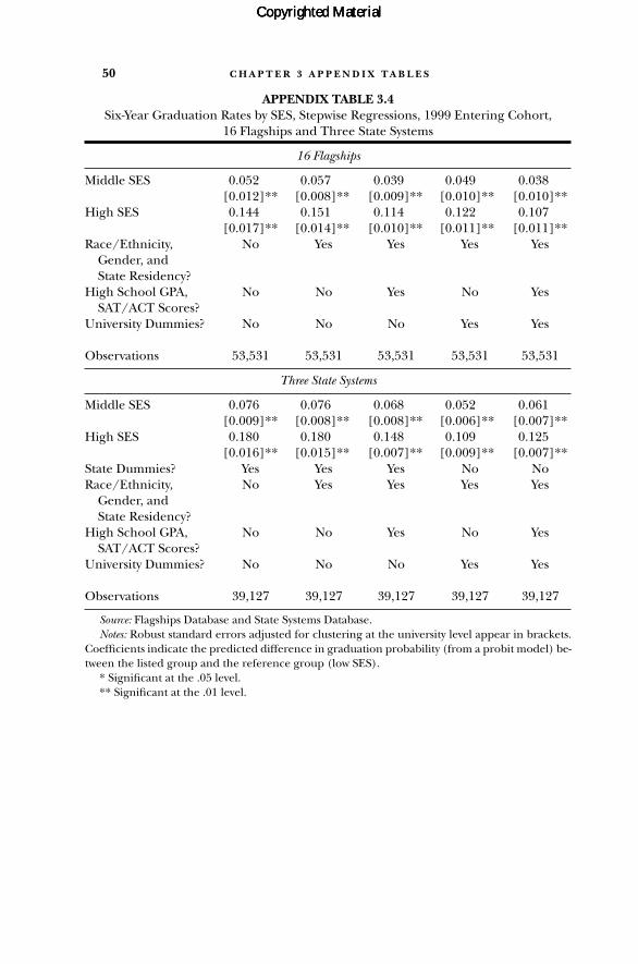
50 C H A P T E R 3 A P P E N D I X T A B L E S
APPENDIX TABLE 3.4Six-Year Graduation Rates by SES, Stepwise Regressions, 1999 Entering Cohort,
16 Flagships and Three State Systems
16 Flagships
Middle SES 0.052 0.057 0.039 0.049 0.038[0.012]** [0.008]** [0.009]** [0.010]** [0.010]**
High SES 0.144 0.151 0.114 0.122 0.107[0.017]** [0.014]** [0.010]** [0.011]** [0.011]**
Race/Ethnicity, No Yes Yes Yes YesGender, and State Residency?
High School GPA, No No Yes No YesSAT/ACT Scores?
University Dummies? No No No Yes Yes
Observations 53,531 53,531 53,531 53,531 53,531
Three State Systems
Middle SES 0.076 0.076 0.068 0.052 0.061[0.009]** [0.008]** [0.008]** [0.006]** [0.007]**
High SES 0.180 0.180 0.148 0.109 0.125[0.016]** [0.015]** [0.007]** [0.009]** [0.007]**
State Dummies? Yes Yes Yes No NoRace/Ethnicity, No Yes Yes Yes Yes
Gender, and State Residency?
High School GPA, No No Yes No YesSAT/ACT Scores?
University Dummies? No No No Yes Yes
Observations 39,127 39,127 39,127 39,127 39,127
Source: Flagships Database and State Systems Database.Notes: Robust standard errors adjusted for clustering at the university level appear in brackets.
Coefficients indicate the predicted difference in graduation probability (from a probit model) be-tween the listed group and the reference group (low SES).
* Significant at the .05 level.** Significant at the .01 level.
Copyrighted MaterialCopyrighted MaterialCopyrighted Material
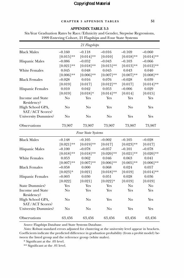
C H A P T E R 3 A P P E N D I X T A B L E S 51
APPENDIX TABLE 3.5Six-Year Graduation Rates by Race/Ethnicity and Gender, Stepwise Regressions,
1999 Entering Cohort, 21 Flagships and Four State Systems
21 Flagships
Black Males –0.160 –0.118 –0.016 –0.169 –0.060[0.015]** [0.014]** [0.010] [0.018]** [0.014]**
Hispanic Males –0.086 –0.052 –0.043 –0.103 –0.066[0.021]** [0.018]** [0.015]** [0.013]** [0.012]**
White Females 0.045 0.048 0.045 0.043 0.040[0.006]** [0.006]** [0.007]** [0.007]** [0.008]**
Black Females –0.028 0.016 0.076 –0.028 0.039[0.019] [0.017] [0.012]** [0.017] [0.014]**
Hispanic Females 0.010 0.042 0.053 –0.006 0.029[0.019] [0.018]* [0.014]** [0.014] [0.015]
Income and State No Yes Yes Yes YesResidency?
High School GPA, No No Yes No YesSAT/ACT Scores?
University Dummies? No No No Yes Yes
Observations 73,907 73,907 73,907 73,907 73,907
Four State Systems
Black Males –0.148 –0.105 –0.002 –0.105 –0.028[0.021]** [0.019]** [0.017] [0.023]** [0.017]
Hispanic Males –0.100 –0.078 –0.057 –0.101 –0.078[0.018]** [0.018]** [0.020]** [0.021]** [0.020]**
White Females 0.053 0.062 0.046 0.063 0.041[0.007]** [0.007]** [0.006]** [0.005]** [0.006]**
Black Females –0.058 0.000 0.068 0.024 0.057[0.023]* [0.021] [0.018]** [0.019] [0.014]**
Hispanic Females –0.003 0.030 0.051 0.028 0.036[0.022] [0.021] [0.022]* [0.019] [0.019]
State Dummies? Yes Yes Yes No NoIncome and State No Yes Yes Yes Yes
Residency?High School GPA, No No Yes No Yes
SAT/ACT Scores?University Dummies? No No No Yes Yes
Observations 63,456 63,456 63,456 63,456 63,456
Source: Flagships Database and State Systems Database.Notes: Robust standard errors adjusted for clustering at the university level appear in brackets.
Coefficients indicate the predicted difference in graduation probability (from a probit model) be-tween the listed group and the reference group (white males).
* Significant at the .05 level.** Significant at the .01 level.
Copyrighted MaterialCopyrighted MaterialCopyrighted Material
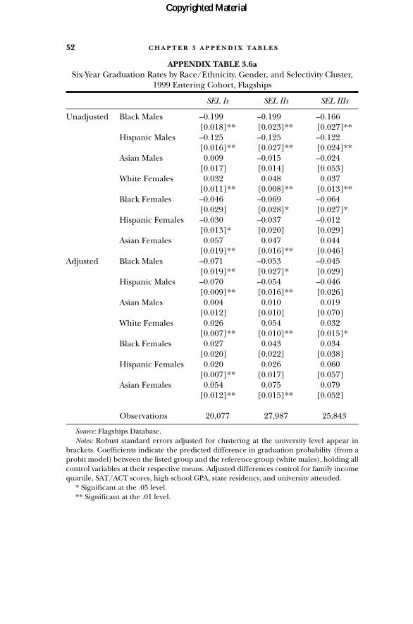
52 C H A P T E R 3 A P P E N D I X T A B L E S
APPENDIX TABLE 3.6aSix-Year Graduation Rates by Race/Ethnicity, Gender, and Selectivity Cluster,
1999 Entering Cohort, Flagships
SEL Is SEL IIs SEL IIIs
Unadjusted Black Males –0.199 –0.199 –0.166[0.018]** [0.023]** [0.027]**
Hispanic Males –0.125 –0.125 –0.122[0.016]** [0.027]** [0.024]**
Asian Males 0.009 –0.015 –0.024[0.017] [0.014] [0.053]
White Females 0.032 0.048 0.037[0.011]** [0.008]** [0.013]**
Black Females –0.046 –0.069 –0.064[0.029] [0.028]* [0.027]*
Hispanic Females –0.030 –0.037 –0.012[0.013]* [0.020] [0.029]
Asian Females 0.057 0.047 0.044[0.019]** [0.016]** [0.046]
Adjusted Black Males –0.071 –0.053 –0.045[0.019]** [0.027]* [0.029]
Hispanic Males –0.070 –0.054 –0.046[0.009]** [0.016]** [0.026]
Asian Males 0.004 0.010 0.019[0.012] [0.010] [0.070]
White Females 0.026 0.054 0.032[0.007]** [0.010]** [0.015]*
Black Females 0.027 0.043 0.034[0.020] [0.022] [0.038]
Hispanic Females 0.020 0.026 0.060[0.007]** [0.017] [0.057]
Asian Females 0.054 0.075 0.079[0.012]** [0.015]** [0.052]
Observations 20,077 27,987 25,843
Source: Flagships Database.Notes: Robust standard errors adjusted for clustering at the university level appear in
brackets. Coefficients indicate the predicted difference in graduation probability (from aprobit model) between the listed group and the reference group (white males), holding allcontrol variables at their respective means. Adjusted differences control for family incomequartile, SAT/ACT scores, high school GPA, state residency, and university attended.
* Significant at the .05 level.** Significant at the .01 level.
Copyrighted MaterialCopyrighted MaterialCopyrighted Material

AP
PE
ND
IX T
AB
LE
3.6
bSi
x-Ye
ar G
radu
atio
n R
ates
by
Rac
e, G
ende
r, an
d Se
lect
ivit
y C
lust
er, 1
999
En
teri
ng
Coh
ort,
Stat
e Sy
stem
s
Mar
ylan
dN
orth
Car
olin
aO
hio
Virg
inia
SEL
As
SEL
Bs
SEL
As
SEL
Bs
SEL
As
SEL
Bs
SEL
As
SEL
Bs
Un
adju
sted
Bla
ck M
ales
–0.1
15–0
.147
–0.1
88–0
.013
–0.1
90–0
.208
–0.1
22–0
.032
[0.0
39]*
*[0
.053
]**
[0.0
20]*
*[0
.041
][0
.063
]**
[0.0
36]*
*[0
.017
]**
[0.0
30]
Wh
ite
Fem
ales
0.05
80.
101
0.07
00.
061
0.06
10.
066
0.03
80.
079
[0.0
25]*
[0.0
26]*
*[0
.007
]**
[0.0
15]*
*[0
.019
]**
[0.0
09]*
*[0
.019
]*[0
.032
]*B
lack
Fem
ales
0.02
20.
048
0.03
30.
061
–0.0
98–0
.160
0.05
50.
020
[0.0
58]
[0.0
35]
[0.0
30]
[0.0
39]
[0.0
45]*
[0.0
32]*
*[0
.022
]*[0
.038
]A
djus
ted
Bla
ck M
ales
–0.0
27–0
.076
–0.0
960.
086
–0.0
20–0
.067
–0.0
63–0
.013
[0.0
22]
[0.0
35]*
[0.0
09]*
*[0
.034
]*[0
.033
][0
.032
]*[0
.017
]**
[0.0
22]
Wh
ite
Fem
ales
0.04
10.
066
0.03
40.
020
0.04
70.
047
0.01
90.
044
[0.0
09]*
*[0
.030
]*[0
.013
]**
[0.0
14]
[0.0
20]*
[0.0
08]*
*[0
.011
][0
.026
]B
lack
Fem
ales
0.08
20.
081
0.05
90.
118
0.04
7–0
.022
0.05
50.
026
[0.0
35]*
[0.0
14]*
*[0
.025
]*[0
.032
]**
[0.0
01]*
*[0
.021
][0
.016
]**
[0.0
26]
Obs
erva
tion
s4,
039
2,85
56,
371
9,75
06,
770
17,5
599,
696
6,41
6
Sour
ce:S
tate
Sys
tem
s D
atab
ase.
Not
es:R
obus
t sta
nda
rd e
rror
s adj
uste
d fo
r cl
uste
rin
g at
the
univ
ersi
ty le
vel a
ppea
r in
bra
cket
s. C
oeffi
cien
ts in
dica
te th
e pr
edic
ted
diff
eren
ce in
gra
d-ua
tion
pro
babi
lity
(fro
m a
pro
bit
mod
el)
betw
een
th
e lis
ted
grou
p an
d th
e re
fere
nce
gro
up (
wh
ite
mal
es),
hol
din
g al
l con
trol
var
iabl
es a
t th
eir
re-
spec
tive
mea
ns.
Adj
uste
d di
ffer
ence
s co
ntr
ol fo
r fa
mily
inco
me
quar
tile
, SA
T/A
CT
sco
res,
hig
h s
choo
l GPA
, sta
te r
esid
ency
, an
d un
iver
sity
att
ende
d.*
Sign
ifica
nt a
t th
e .0
5 le
vel.
** S
ign
ifica
nt a
t th
e .0
1 le
vel.
Copyrighted MaterialCopyrighted MaterialCopyrighted Material

54 C H A P T E R 3 A P P E N D I X T A B L E S
APPENDIX TABLE 3.7aTransfer Graduation Rates by Socioeconomic Status and Selectivity Cluster,
1999 Entering Cohort, 16 Flagships and Three State Systems (Percent)
All Low SES Middle SES High SES
Flagship SEL Is 3.3 2.6 3.5 3.4Flagship SEL IIs 4.6 4.1 4.9 4.6Flagship SEL IIIs 3.9 4.3 4.1 3.7State System SEL As 7.0 7.2 7.5 6.8State System SEL Bs 14.2 11.6 13.6 16.1All 16 Flagships 3.9 3.7 4.2 3.8All Three State Systems 10.5 10.2 11.1 10.3
Source: Flagships Database and State Systems Database.Notes: Each cell indicates the percentage of all students in a given subgroup who appear
in the Clearinghouse data as having received a four-year degree but did not graduate fromtheir original institution. Ohio is excluded from state systems because Clearinghouse dataare not available. The five flagships without parental education data available are excluded.
APPENDIX TABLE 3.7bTransfer Graduation Rates by Race, Gender, and Selectivity Cluster, 1999
Entering Cohort, 21 Flagships and Three State Systems (Percent)
White Black White BlackAll Males Males Females Females
Flagship SEL I 3.3 3.0 3.2 4.5 3.1Flagship SEL IIs 5.0 4.7 4.5 5.7 5.6Flagship SEL IIIs 6.3 5.4 3.8 7.2 4.6State System SEL As 7.0 6.2 7.0 8.1 5.1State System SEL Bs 14.2 14.4 11.7 15.2 10.1All Flagships 5.0 4.6 3.8 6.0 4.4All Three State Systems 10.5 9.9 9.4 11.7 8.2
Source: Flagships Database and State Systems Database.Notes: Each cell indicates the percentage of all students in a given subgroup that appear
in the Clearinghouse data as having received a four-year degree but did not graduate fromtheir original institution. Ohio is excluded from state systems because Clearinghouse dataare not available.
Copyrighted MaterialCopyrighted MaterialCopyrighted Material

C H A P T E R 3 A P P E N D I X T A B L E S 55
APPENDIX TABLE 3.8Six-Year Graduation Rates by First-Year GPA and Selectivity Cluster,
1999 Entering Cohort, Flagships and State System SEL Bs
Flagship SEL Is Flagship SEL IIs
First-Year GPA 0.150 0.140 0.205 0.197[0.003]** [0.005]** [0.009]** [0.009]**
Controls? No Yes No Yes
Observations 19,495 19,495 20,529 20,529
Flagship SEL IIIs State System SEL Bs
First-Year GPA 0.313 0.304 0.298 0.287[0.017]** [0.017]** [0.018]** [0.015]**
Controls? No Yes No Yes
Observations 24,383 24,383 33,404 33,404
Source: Flagships Database and State Systems Database.Notes: Robust standard errors in brackets. Coefficients indicate the predicted difference
in graduation probability (from a probit model) associated with increasing first-year GPAby 1 point, holding all control variables at their respective means. All regressions includeuniversity dummy variables. Controls include race/ethnicity, gender, SAT/ACT scores, highschool GPA, state residency status, and family income quartile.
* Significant at the .05 level.** Significant at the .01 level.
Copyrighted MaterialCopyrighted MaterialCopyrighted Material

56 C H A P T E R 3 A P P E N D I X T A B L E S
APPENDIX TABLE 3.9Six-Year Graduation Rates by Family Income, 1999 Entering Cohort,
Flagships and State System SEL Bs
Flagships State System SEL Bs
Second Quartile 0.016 0.019 0.036 0.023[0.009] [0.007]* [0.014]* [0.012]
Third Quartile 0.042 0.037 0.079 0.062[0.010]** [0.008]** [0.011]** [0.010]**
Top Quartile 0.079 0.063 0.105 0.085[0.010]** [0.007]** [0.011]** [0.010]**
Standard Controls? Yes Yes Yes YesFirst-Year GPA? No Yes No Yes
Observations 64,407 64,407 33,404 33,404
Source: Flagships Database and State Systems Database.Notes: Robust standard errors adjusted for clustering at the university level appear in
brackets. Coefficients indicate the predicted difference in graduation probability (from aprobit model) between the listed group and the reference group (students from familiesin the bottom income quartile), holding all control variables at their respective means. Stan-dard controls include SAT/ACT scores, high school GPA, state residency, race/ethnicity,gender, and university attended.
* Significant at the .05 level.** Significant at the .01 level.
Copyrighted MaterialCopyrighted MaterialCopyrighted Material

C H A P T E R 3 A P P E N D I X T A B L E S 57
APPENDIX TABLE 3.10Six-Year Graduation Rates by Race/Ethnicity and Gender, 1999 Entering
Cohort, Flagships and State System SEL Bs
Flagships State System SEL Bs
Black Males –0.076 –0.060 –0.026 –0.017[0.013]** [0.015]** [0.024] [0.020]
Hispanic Males –0.066 –0.037 –0.074 –0.062[0.014]** [0.012]** [0.036]* [0.037]
White Females 0.040 –0.002 0.047 0.002[0.008]** [0.009] [0.008]** [0.008]
Black Females 0.023 0.017 0.037 0.035[0.013] [0.014] [0.021] [0.020]
Hispanic Females 0.024 0.004 0.029 0.008[0.016] [0.016] [0.027] [0.028]
Standard Controls? Yes Yes Yes YesFirst-Year GPA? No Yes No Yes
Observations 64,407 64,407 33,404 33,404
Source: Flagships Database and State Systems Database.Notes: Robust standard errors adjusted for clustering at the university level appear in
brackets. Coefficients indicate the predicted difference in graduation probability (from aprobit model) between the listed group and the reference group (white males), holding allcontrol variables at their respective means. Standard controls include SAT/ACT scores,high school GPA, state residency, family income quartile, and university attended.
* Significant at the .05 level.** Significant at the .01 level.
Copyrighted MaterialCopyrighted MaterialCopyrighted Material

AP
PE
ND
IX T
AB
LE
4.1
aA
djus
ted
Maj
or a
t Gra
duat
ion
by
Soci
oeco
nom
ic S
tatu
s, 1
999
En
teri
ng
Coh
ort,
Flag
ship
s
Engi
neer
ing,
Mat
h, a
ndC
omm
unic
atio
nsPr
ofes
sion
alPh
ysic
al S
cien
ces
Life
Sci
ence
sH
uman
ities
Soci
al S
cien
ces
and
Educ
atio
nB
usin
ess
and
Oth
er
Mid
dle
SES
–0.0
100.
002
0.01
7–0
.027
0.00
90.
018
–0.0
09[0
.007
][0
.006
][0
.006
]**
[0.0
09]*
*[0
.004
]*[0
.006
]**
[0.0
06]
Hig
h S
ES
–0.0
06–0
.006
0.01
4–0
.036
0.01
50.
036
–0.0
16[0
.007
][0
.005
][0
.005
]*[0
.008
]**
[0.0
04]*
*[0
.006
]**
[0.0
06]*
*
Obs
erva
tion
s40
,539
40,5
3940
,539
40,5
3940
,539
40,5
3940
,539
Sour
ce:F
lags
hip
s D
atab
ase.
Not
es:S
tan
dard
err
ors
appe
ar in
bra
cket
s. T
he
repo
rted
coe
ffici
ents
are
mar
gin
al e
ffec
ts f
rom
a m
ulti
nom
ial l
ogit
mod
el, w
hic
h in
dica
te t
he
pre-
dict
ed d
iffe
ren
ce in
the
prob
abili
ty o
f ch
oosi
ng
a gi
ven
maj
or b
etw
een
the
liste
d gr
oup
and
the
refe
ren
ce g
roup
(lo
w-S
ES
stud
ents
), h
oldi
ng
all c
on-
trol
var
iabl
es c
onst
ant a
t th
eir
mea
ns.
Con
trol
var
iabl
es in
clud
e h
igh
sch
ool G
PA, S
AT
/AC
T s
core
s, r
ace/
eth
nic
ity,
gen
der,
stat
e re
side
ncy
sta
tus,
an
din
stit
utio
n a
tten
ded.
* Si
gnifi
can
t at t
he
.05
leve
l.**
Sig
nifi
can
t at t
he
.01
leve
l.
Copyrighted MaterialCopyrighted MaterialCopyrighted Material

AP
PE
ND
IX T
AB
LE
4.1
bA
djus
ted
Maj
or a
t Gra
duat
ion
by
Soci
oeco
nom
ic S
tatu
s an
d Se
lect
ivit
y C
lust
er, 1
999
En
teri
ng
Coh
ort,
Stat
e Sy
stem
s
SEL
As
Engi
neer
ing,
M
ath,
and
C
omm
unic
atio
nsPr
ofes
sion
alPh
ysic
al S
cien
ces
Life
Sci
ence
sH
uman
ities
Soci
al S
cien
ces
and
Educ
atio
nB
usin
ess
and
Oth
er
Mid
dle
SES
0.01
30.
003
0.01
0–0
.039
–0.0
010.
010
0.00
4[0
.014
][0
.011
][0
.013
][0
.017
]*[0
.007
][0
.013
][0
.009
]H
igh
SE
S0.
003
–0.0
020.
003
–0.0
450.
007
0.03
30.
001
[0.0
13]
[0.0
10]
[0.0
12]
[0.0
16]*
*[0
.007
][0
.012
]**
[0.0
08]
Obs
erva
tion
s15
,021
15,0
2115
,021
15,0
2115
,021
15,0
2115
,021
SEL
Bs
Engi
neer
ing,
M
ath,
and
C
omm
unic
atio
nsPr
ofes
sion
alPh
ysic
al S
cien
ces
Life
Sci
ence
sH
uman
ities
Soci
al S
cien
ces
and
Educ
atio
nB
usin
ess
and
Oth
er
Mid
dle
SES
–0.0
060.
006
0.02
2–0
.027
–0.0
060.
002
0.00
9[0
.007
][0
.005
][0
.011
]*[0
.012
]*[0
.010
][0
.013
][0
.011
]H
igh
SE
S–0
.008
0.00
70.
044
–0.0
29–0
.011
–0.0
03–0
.001
[0.0
07]
[0.0
05]
[0.0
11]*
*[0
.012
]*[0
.010
][0
.013
][0
.011
]
Obs
erva
tion
s9,
940
9,94
09,
940
9,94
09,
940
9,94
09,
940
Sour
ce:S
tate
Sys
tem
s D
atab
ase.
Not
es:S
tan
dard
err
ors
appe
ar in
bra
cket
s. T
he
repo
rted
coe
ffici
ents
are
mar
gin
al e
ffec
ts f
rom
a m
ulti
nom
ial l
ogit
mod
el, w
hic
h in
dica
te t
he
pre-
dict
ed d
iffe
ren
ce in
the
prob
abili
ty o
f ch
oosi
ng
a gi
ven
maj
or b
etw
een
the
liste
d gr
oup
and
the
refe
ren
ce g
roup
(lo
w-S
ES
stud
ents
), h
oldi
ng
all c
on-
trol
var
iabl
es c
onst
ant a
t th
eir
mea
ns.
Con
trol
var
iabl
es in
clud
e h
igh
sch
ool G
PA, S
AT
/AC
T s
core
s, r
ace/
eth
nic
ity,
gen
der,
stat
e re
side
ncy
sta
tus,
an
din
stit
utio
n a
tten
ded.
* Si
gnifi
can
t at t
he
.05
leve
l.**
Sig
nifi
can
t at t
he
.01
leve
l.
Copyrighted MaterialCopyrighted MaterialCopyrighted Material
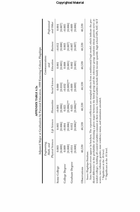
AP
PE
ND
IX T
AB
LE
4.2
aA
djus
ted
Maj
or a
t Gra
duat
ion
by
Pare
nta
l Edu
cati
on, 1
999
En
teri
ng
Coh
ort,
Flag
ship
s
Engi
neer
ing,
C
omm
unic
atio
nsM
ath,
and
an
dPr
ofes
sion
alPh
ysic
al S
cien
ces
Life
Sci
ence
sH
uman
ities
Soci
al S
cien
ces
Educ
atio
nB
usin
ess
and
Oth
er
Som
e C
olle
ge0.
003
0.00
5–0
.001
0.00
00.
001
–0.0
120.
004
[0.0
09]
[0.0
06]
[0.0
06]
[0.0
10]
[0.0
05]
[0.0
08]
[0.0
07]
Col
lege
Deg
ree
0.00
9–0
.004
0.02
1–0
.032
0.00
80.
003
–0.0
05[0
.008
][0
.006
][0
.006
]**
[0.0
09]*
*[0
.005
][0
.007
][0
.006
]G
radu
ate
Deg
ree
–0.0
140.
012
0.02
5–0
.009
0.00
2–0
.007
–0.0
09[0
.008
][0
.006
]*[0
.006
]**
[0.0
09]
[0.0
05]
[0.0
07]
[0.0
06]
Obs
erva
tion
s40
,539
40,5
3940
,539
40,5
3940
,539
40,5
3940
,539
Sour
ce:F
lags
hip
s D
atab
ase.
Not
es:S
tan
dard
err
ors
appe
ar in
bra
cket
s. T
he
repo
rted
coe
ffici
ents
are
mar
gin
al e
ffec
ts f
rom
a m
ulti
nom
ial l
ogit
mod
el, w
hic
h in
dica
te t
he
pre-
dict
ed d
iffe
ren
ce i
n t
he
prob
abili
ty o
f ch
oosi
ng
a gi
ven
maj
or b
etw
een
th
e lis
ted
grou
p an
d th
e re
fere
nce
gro
up (
stud
ents
wh
ose
pare
nts
nev
er a
t-te
nde
d co
llege
), h
oldi
ng
all c
ontr
ol v
aria
bles
con
stan
t at
th
eir
mea
ns.
Con
trol
var
iabl
es in
clud
e fa
mily
inco
me
quar
tile
, hig
h s
choo
l GPA
, SA
T/A
CT
scor
es, r
ace/
eth
nic
ity,
gen
der,
stat
e re
side
ncy
sta
tus,
an
d in
stit
utio
n a
tten
ded.
* Si
gnifi
can
t at t
he
.05
leve
l.**
Sig
nifi
can
t at t
he
.01
leve
l.
Copyrighted MaterialCopyrighted MaterialCopyrighted Material

AP
PE
ND
IX T
AB
LE
4.2
bA
djus
ted
Maj
or a
t Gra
duat
ion
by
Pare
nta
l Edu
cati
on a
nd
Sele
ctiv
ity
Clu
ster
, 199
9 E
nte
rin
g C
ohor
t, St
ate
Syst
ems
SEL
As
Engi
neer
ing,
C
omm
unic
atio
nsM
ath,
and
an
dPr
ofes
sion
alPh
ysic
al S
cien
ces
Life
Sci
ence
sH
uman
ities
Soci
al S
cien
ces
Educ
atio
nB
usin
ess
and
Oth
er
Som
e C
olle
ge–0
.017
0.02
90.
001
0.00
6–0
.003
–0.0
07–0
.009
[0.0
16]
[0.0
12]*
[0.0
13]
[0.0
18]
[0.0
08]
[0.0
15]
[0.0
10]
Col
lege
Deg
ree
–0.0
210.
010
0.01
8–0
.003
0.00
60.
000
–0.0
09[0
.014
][0
.010
][0
.011
][0
.017
][0
.007
][0
.014
][0
.009
]G
radu
ate
Deg
ree
–0.0
330.
022
0.03
10.
003
0.00
4–0
.018
–0.0
09[0
.015
]*[0
.010
]*[0
.012
]**
[0.0
17]
[0.0
07]
[0.0
14]
[0.0
09]
Obs
erva
tion
s15
,021
15,0
2115
,021
15,0
2115
,021
15,0
2115
,021
SEL
Bs
Engi
neer
ing,
C
omm
unic
atio
nsM
ath,
and
an
dPr
ofes
sion
alPh
ysic
al S
cien
ces
Life
Sci
ence
sH
uman
ities
Soci
al S
cien
ces
Educ
atio
nB
usin
ess
and
Oth
er
Som
e C
olle
ge–0
.001
–0.0
020.
023
0.00
2–0
.001
–0.0
14–0
.007
[0.0
08]
[0.0
06]
[0.0
12]
[0.0
14]
[0.0
11]
[0.0
15]
[0.0
12]
Col
lege
Deg
ree
–0.0
080.
004
0.03
7–0
.025
0.00
5–0
.021
0.00
7[0
.007
][0
.006
][0
.012
]**
[0.0
13]
[0.0
11]
[0.0
14]
[0.0
12]
Gra
duat
e D
egre
e0.
000
0.00
60.
054
–0.0
100.
003
–0.0
50–0
.003
[0.0
08]
[0.0
06]
[0.0
13]*
*[0
.014
][0
.012
][0
.015
]**
[0.0
13]
Obs
erva
tion
s9,
940
9,94
09,
940
9,94
09,
940
9,94
09,
940
Sour
ce:S
tate
Sys
tem
s D
atab
ase.
Not
es:S
tan
dard
err
ors
appe
ar in
bra
cket
s. T
he
repo
rted
coe
ffici
ents
are
mar
gin
al e
ffec
ts f
rom
a m
ulti
nom
ial l
ogit
mod
el, w
hic
h in
dica
te t
he
pre-
dict
ed d
iffe
ren
ce i
n t
he
prob
abili
ty o
f ch
oosi
ng
a gi
ven
maj
or b
etw
een
th
e lis
ted
grou
p an
d th
e re
fere
nce
gro
up (
stud
ents
wh
ose
pare
nts
nev
er a
t-te
nde
d co
llege
), h
oldi
ng
all c
ontr
ol v
aria
bles
con
stan
t at
th
eir
mea
ns.
Con
trol
var
iabl
es in
clud
e fa
mily
inco
me
quar
tile
, hig
h s
choo
l GPA
, SA
T/A
CT
scor
es, r
ace/
eth
nic
ity,
gen
der,
stat
e re
side
ncy
sta
tus,
an
d in
stit
utio
n a
tten
ded.
* Si
gnifi
can
t at t
he
.05
leve
l.**
Sig
nifi
can
t at t
he
.01
leve
l.
Copyrighted MaterialCopyrighted MaterialCopyrighted Material
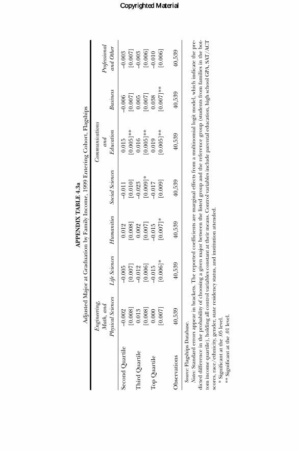
AP
PE
ND
IX T
AB
LE
4.3
aA
djus
ted
Maj
or a
t Gra
duat
ion
by
Fam
ily I
nco
me,
199
9 E
nte
rin
g C
ohor
t, Fl
agsh
ips
Engi
neer
ing,
C
omm
unic
atio
nsM
ath,
and
an
dPr
ofes
sion
alPh
ysic
al S
cien
ces
Life
Sci
ence
sH
uman
ities
Soci
al S
cien
ces
Educ
atio
nB
usin
ess
and
Oth
er
Seco
nd
Qua
rtile
–0.0
02–0
.005
0.01
2–0
.011
0.01
5–0
.006
–0.0
03[0
.008
][0
.007
][0
.008
][0
.010
][0
.005
]**
[0.0
07]
[0.0
07]
Th
ird
Qua
rtile
0.01
3–0
.012
0.00
2–0
.023
0.01
60.
005
–0.0
03[0
.008
][0
.006
][0
.007
][0
.009
]*[0
.005
]**
[0.0
07]
[0.0
06]
Top
Qua
rtile
0.00
0–0
.015
–0.0
15–0
.017
0.01
90.
038
–0.0
10[0
.007
][0
.006
]*[0
.007
]*[0
.009
][0
.005
]**
[0.0
07]*
*[0
.006
]
Obs
erva
tion
s40
,539
40,5
3940
,539
40,5
3940
,539
40,5
3940
,539
Sour
ce:F
lags
hip
s D
atab
ase.
Not
es:S
tan
dard
err
ors
appe
ar in
bra
cket
s. T
he
repo
rted
coe
ffici
ents
are
mar
gin
al e
ffec
ts f
rom
a m
ulti
nom
ial l
ogit
mod
el, w
hic
h in
dica
te t
he
pre-
dict
ed d
iffe
ren
ce in
th
e pr
obab
ility
of
choo
sin
g a
give
n m
ajor
bet
wee
n t
he
liste
d gr
oup
and
the
refe
ren
ce g
roup
(st
uden
ts f
rom
fam
ilies
in t
he
bot-
tom
inco
me
quar
tile
), h
oldi
ng
all c
ontr
ol v
aria
bles
con
stan
t at t
hei
r m
ean
s. C
ontr
ol v
aria
bles
incl
ude
pare
nta
l edu
cati
on, h
igh
sch
ool G
PA, S
AT
/AC
Tsc
ores
, rac
e/et
hn
icit
y, g
ende
r, st
ate
resi
den
cy s
tatu
s, a
nd
inst
itut
ion
att
ende
d.*
Sign
ifica
nt a
t th
e .0
5 le
vel.
** S
ign
ifica
nt a
t th
e .0
1 le
vel.
Copyrighted MaterialCopyrighted MaterialCopyrighted Material

AP
PE
ND
IX T
AB
LE
4.3
bA
djus
ted
Maj
or a
t Gra
duat
ion
by
Fam
ily I
nco
me
and
Sele
ctiv
ity
Clu
ster
, 199
9 E
nte
rin
g C
ohor
t, St
ate
Syst
ems
SEL
As
Engi
neer
ing,
C
omm
unic
atio
nsM
ath,
and
an
dPr
ofes
sion
alPh
ysic
al S
cien
ces
Life
Sci
ence
sH
uman
ities
Soci
al S
cien
ces
Educ
atio
nB
usin
ess
and
Oth
er
Seco
nd
Qua
rtile
0.01
0–0
.016
–0.0
140.
025
0.01
2–0
.017
0.00
0[0
.016
][0
.014
][0
.018
][0
.021
][0
.009
][0
.016
][0
.011
]T
hir
d Q
uart
ile0.
026
–0.0
16–0
.021
–0.0
080.
012
–0.0
040.
011
[0.0
15]
[0.0
13]
[0.0
17]
[0.0
19]
[0.0
08]
[0.0
15]
[0.0
10]
Top
Qua
rtile
0.02
0–0
.014
–0.0
47–0
.016
0.01
20.
044
0.00
0[0
.015
][0
.013
][0
.016
]**
[0.0
19]
[0.0
08]
[0.0
15]*
*[0
.010
]
Obs
erva
tion
s15
,021
15,0
2115
,021
15,0
2115
,021
15,0
2115
,021
SEL
Bs
Engi
neer
ing,
C
omm
unic
atio
nsM
ath,
and
an
dPr
ofes
sion
alPh
ysic
al S
cien
ces
Life
Sci
ence
sH
uman
ities
Soci
al S
cien
ces
Educ
atio
nB
usin
ess
and
Oth
er
Seco
nd
Qua
rtile
–0.0
18–0
.002
0.01
5–0
.008
0.00
9–0
.020
0.02
4[0
.009
]*[0
.007
][0
.014
][0
.015
][0
.013
][0
.016
][0
.014
]T
hir
d Q
uart
ile–0
.020
–0.0
020.
036
–0.0
10–0
.006
–0.0
140.
016
[0.0
09]*
[0.0
07]
[0.0
14]*
*[0
.015
][0
.013
][0
.016
][0
.014
]To
p Q
uart
ile–0
.013
–0.0
010.
014
–0.0
09–0
.014
0.02
5–0
.002
[0.0
09]
[0.0
07]
[0.0
14]
[0.0
15]
[0.0
13]
[0.0
17]
[0.0
14]
Obs
erva
tion
s9,
940
9,94
09,
940
9,94
09,
940
9,94
09,
940
Sour
ce:S
tate
Sys
tem
s D
atab
ase.
Not
es:S
tan
dard
err
ors
appe
ar in
bra
cket
s. T
he
repo
rted
coe
ffici
ents
are
mar
gin
al e
ffec
ts f
rom
a m
ulti
nom
ial l
ogit
mod
el, w
hic
h in
dica
te t
he
pre-
dict
ed d
iffe
ren
ce in
th
e pr
obab
ility
of
choo
sin
g a
give
n m
ajor
bet
wee
n t
he
liste
d gr
oup
and
the
refe
ren
ce g
roup
(st
uden
ts f
rom
fam
ilies
in t
he
bot-
tom
inco
me
quar
tile
), h
oldi
ng
all c
ontr
ol v
aria
bles
con
stan
t at t
hei
r m
ean
s. C
ontr
ol v
aria
bles
incl
ude
pare
nta
l edu
cati
on, h
igh
sch
ool G
PA, S
AT
/AC
Tsc
ores
, rac
e/et
hn
icit
y, g
ende
r, st
ate
resi
den
cy s
tatu
s, a
nd
inst
itut
ion
att
ende
d.*
Sign
ifica
nt a
t th
e .0
5 le
vel.
** S
ign
ifica
nt a
t th
e .0
1 le
vel.
Copyrighted MaterialCopyrighted MaterialCopyrighted Material

AP
PE
ND
IX T
AB
LE
4.4
aU
nad
just
ed M
ajor
at G
radu
atio
n b
y R
ace/
Eth
nic
ity
and
Gen
der,
1999
En
teri
ng
Coh
ort,
Flag
ship
s
Engi
neer
ing,
C
omm
unic
atio
nsM
ath,
and
an
dPr
ofes
sion
alPh
ysic
al S
cien
ces
Life
Sci
ence
sH
uman
ities
Soci
al S
cien
ces
Educ
atio
nB
usin
ess
and
Oth
er
Bla
ck M
ales
–0.1
14–0
.010
0.00
60.
101
0.02
3–0
.039
0.03
2[0
.014
]**
[0.0
08]
[0.0
10]
[0.0
15]*
*[0
.009
]*[0
.011
]**
[0.0
11]*
*H
ispa
nic
Mal
es–0
.076
0.01
20.
022
0.07
20.
007
–0.0
32–0
.004
[0.0
13]*
*[0
.008
][0
.009
]*[0
.013
]**
[0.0
08]
[0.0
11]*
*[0
.008
]A
sian
Mal
es0.
089
0.04
4–0
.046
0.00
9–0
.045
–0.0
40–0
.011
[0.0
09]*
*[0
.006
]**
[0.0
04]*
*[0
.007
][0
.003
]**
[0.0
06]*
*[0
.005
]*W
hit
e Fe
mal
es–0
.237
0.01
70.
057
0.02
00.
111
–0.0
510.
082
[0.0
04]*
*[0
.003
]**
[0.0
03]*
*[0
.004
]**
[0.0
03]*
*[0
.003
]**
[0.0
03]*
*B
lack
Fem
ales
–0.2
53–0
.005
0.04
50.
108
0.07
1–0
.075
0.10
9[0
.007
]**
[0.0
06]
[0.0
08]*
*[0
.011
]**
[0.0
08]*
*[0
.007
]**
[0.0
09]*
*H
ispa
nic
Fem
ales
–0.2
440.
012
0.05
90.
131
0.05
4–0
.075
0.06
3[0
.008
]**
[0.0
07]
[0.0
09]*
*[0
.012
]**
[0.0
09]*
*[0
.008
]**
[0.0
09]*
*A
sian
Fem
ales
–0.1
660.
080
0.00
20.
068
0.00
4–0
.031
0.04
2[0
.007
]**
[0.0
06]*
*[0
.005
][0
.008
]**
[0.0
04]
[0.0
06]*
*[0
.006
]**
Obs
erva
tion
s55
,342
55,3
4255
,342
55,3
4255
,342
55,3
4255
,342
Sour
ce:F
lags
hip
s D
atab
ase.
Not
es:S
tan
dard
err
ors
appe
ar in
bra
cket
s. T
he
repo
rted
coe
ffici
ents
are
mar
gin
al e
ffec
ts f
rom
a m
ulti
nom
ial l
ogit
mod
el, w
hic
h in
dica
te t
he
pre-
dict
ed d
iffe
ren
ce in
the
prob
abili
ty o
f ch
oosi
ng
a gi
ven
maj
or b
etw
een
the
liste
d gr
oup
and
the
refe
ren
ce g
roup
(w
hit
e m
ales
).*
Sign
ifica
nt a
t th
e .0
5 le
vel.
** S
ign
ifica
nt a
t th
e .0
1 le
vel.
Copyrighted MaterialCopyrighted MaterialCopyrighted Material

AP
PE
ND
IX T
AB
LE
4.4
bA
djus
ted
Maj
or a
t Gra
duat
ion
by
Rac
e/E
thn
icit
y an
d G
ende
r, 19
99 E
nte
rin
g C
ohor
t, Fl
agsh
ips
Engi
neer
ing,
C
omm
unic
atio
nsM
ath,
and
an
dPr
ofes
sion
alPh
ysic
al S
cien
ces
Life
Sci
ence
sH
uman
ities
Soci
al S
cien
ces
Educ
atio
nB
usin
ess
and
Oth
er
Bla
ck M
ales
0.07
00.
015
–0.0
23–0
.027
–0.0
13–0
.021
–0.0
01[0
.020
]**
[0.0
12]
[0.0
09]*
*[0
.014
]*[0
.006
]*[0
.013
][0
.009
]H
ispa
nic
Mal
es0.
014
0.02
00.
009
–0.0
09–0
.001
–0.0
14–0
.019
[0.0
15]
[0.0
10]*
[0.0
10]
[0.0
13]
[0.0
07]
[0.0
12]
[0.0
08]*
Asi
an M
ales
0.03
60.
034
–0.0
45–0
.022
–0.0
300.
026
0.00
1[0
.009
]**
[0.0
06]*
*[0
.005
]**
[0.0
09]*
[0.0
04]*
*[0
.009
]**
[0.0
06]
Wh
ite
Fem
ales
–0.1
750.
018
0.04
5–0
.002
0.08
8–0
.050
0.07
6[0
.004
]**
[0.0
03]*
*[0
.004
]**
[0.0
05]
[0.0
03]*
*[0
.004
]**
[0.0
04]*
*B
lack
Fem
ales
–0.0
980.
031
0.01
7–0
.005
0.02
4–0
.040
0.07
1[0
.014
]**
[0.0
10]*
*[0
.008
]*[0
.011
][0
.006
]**
[0.0
10]*
*[0
.009
]**
His
pan
ic F
emal
es–0
.137
0.03
20.
049
0.03
80.
035
–0.0
550.
038
[0.0
12]*
*[0
.010
]**
[0.0
10]*
*[0
.013
]**
[0.0
08]*
*[0
.010
]**
[0.0
09]*
*A
sian
Fem
ales
–0.1
330.
056
–0.0
06–0
.015
0.03
30.
033
0.03
2[0
.006
]**
[0.0
06]*
*[0
.006
][0
.008
][0
.006
]**
[0.0
09]*
*[0
.006
]**
Obs
erva
tion
s55
,342
55,3
4255
,342
55,3
4255
,342
55,3
4255
,342
Sour
ce:F
lags
hip
s D
atab
ase.
Not
es:S
tan
dard
err
ors
appe
ar in
bra
cket
s. T
he
repo
rted
coe
ffici
ents
are
mar
gin
al e
ffec
ts f
rom
a m
ulti
nom
ial l
ogit
mod
el, w
hic
h in
dica
te t
he
pre-
dict
ed d
iffe
ren
ce in
th
e pr
obab
ility
of
choo
sin
g a
give
n m
ajor
bet
wee
n t
he
liste
d gr
oup
and
the
refe
ren
ce g
roup
(w
hit
e m
ales
), h
oldi
ng
all c
ontr
olva
riab
les
con
stan
t at t
hei
r m
ean
s. C
ontr
ol v
aria
bles
incl
ude
fam
ily in
com
e qu
arti
le, h
igh
sch
ool G
PA, S
AT
/AC
T s
core
s, s
tate
res
iden
cy s
tatu
s, a
nd
in-
stit
utio
n a
tten
ded.
* Si
gnifi
can
t at t
he
.05
leve
l.**
Sig
nifi
can
t at t
he
.01
leve
l.
Copyrighted MaterialCopyrighted MaterialCopyrighted Material

AP
PE
ND
IX T
AB
LE
4.5
aU
nad
just
ed M
ajor
at G
radu
atio
n b
y R
ace,
Gen
der,
and
Sele
ctiv
ity
Clu
ster
, 199
9 E
nte
rin
g C
ohor
t, St
ate
Syst
ems
SEL
As
Engi
neer
ing,
C
omm
unic
atio
nsM
ath,
and
an
dPr
ofes
sion
alPh
ysic
al S
cien
ces
Life
Sci
ence
sH
uman
ities
Soci
al S
cien
ces
Educ
atio
nB
usin
ess
and
Oth
er
Bla
ck M
ales
–0.0
75–0
.018
0.01
00.
089
0.02
8–0
.080
0.04
6[0
.020
]**
[0.0
10]
[0.0
13]
[0.0
20]*
*[0
.013
]*[0
.015
]**
[0.0
14]*
*W
hit
e Fe
mal
es–0
.229
0.02
20.
056
0.02
50.
084
–0.0
560.
098
[0.0
06]*
*[0
.004
]**
[0.0
05]*
*[0
.006
]**
[0.0
05]*
*[0
.006
]**
[0.0
05]*
*B
lack
Fem
ales
–0.2
340.
006
0.03
00.
094
0.09
0–0
.085
0.09
8[0
.010
]**
[0.0
09]
[0.0
11]*
*[0
.015
]**
[0.0
12]*
*[0
.011
]**
[0.0
12]*
*
Obs
erva
tion
s19
,923
19,9
2319
,923
19,9
2319
,923
19,9
2319
,923
SEL
Bs
Engi
neer
ing,
C
omm
unic
atio
nsM
ath,
and
an
dPr
ofes
sion
alPh
ysic
al S
cien
ces
Life
Sci
ence
sH
uman
ities
Soci
al S
cien
ces
Educ
atio
nB
usin
ess
and
Oth
er
Bla
ck M
ales
–0.0
77–0
.008
0.01
60.
033
–0.0
090.
026
0.02
0[0
.016
]**
[0.0
08]
[0.0
16]
[0.0
16]*
[0.0
15]
[0.0
22]
[0.0
16]
Wh
ite
Fem
ales
–0.1
640.
006
0.05
20.
021
0.12
1–0
.134
0.09
8[0
.005
]**
[0.0
03]
[0.0
06]*
*[0
.005
]**
[0.0
06]*
*[0
.007
]**
[0.0
06]*
*B
lack
Fem
ales
–0.1
490.
011
0.01
00.
082
0.01
5–0
.084
0.11
6[0
.008
]**
[0.0
07]
[0.0
11]
[0.0
12]*
*[0
.011
][0
.013
]**
[0.0
13]*
*
Obs
erva
tion
s18
,293
18,2
9318
,293
18,2
9318
,293
18,2
9318
,293
Sour
ce:S
tate
Sys
tem
s D
atab
ase.
Not
es:S
tan
dard
err
ors
appe
ar in
bra
cket
s. T
he
repo
rted
coe
ffici
ents
are
mar
gin
al e
ffec
ts f
rom
a m
ulti
nom
ial l
ogit
mod
el, w
hic
h in
dica
te t
he
pre-
dict
ed d
iffe
ren
ce in
the
prob
abili
ty o
f ch
oosi
ng
a gi
ven
maj
or b
etw
een
the
liste
d gr
oup
and
the
refe
ren
ce g
roup
(w
hit
e m
ales
).*
Sign
ifica
nt a
t th
e .0
5 le
vel.
** S
ign
ifica
nt a
t th
e .0
1 le
vel.
Copyrighted MaterialCopyrighted MaterialCopyrighted Material

AP
PE
ND
IX T
AB
LE
4.5
bA
djus
ted
Maj
or a
t Gra
duat
ion
by
Rac
e, G
ende
r, an
d Se
lect
ivit
y C
lust
er, 1
999
En
teri
ng
Coh
ort,
Stat
e Sy
stem
s
SEL
As
Engi
neer
ing,
C
omm
unic
atio
nsM
ath,
and
an
dPr
ofes
sion
alPh
ysic
al S
cien
ces
Life
Sci
ence
sH
uman
ities
Soci
al S
cien
ces
Educ
atio
nB
usin
ess
and
Oth
er
Bla
ck M
ales
0.08
10.
003
–0.0
05–0
.001
–0.0
15–0
.064
0.00
1[0
.027
]**
[0.0
16]
[0.0
14]
[0.0
21]
[0.0
08]
[0.0
18]*
*[0
.009
]W
hit
e Fe
mal
es–0
.164
0.02
20.
047
0.00
10.
063
–0.0
580.
090
[0.0
06]*
*[0
.005
]**
[0.0
06]*
*[0
.008
][0
.005
]**
[0.0
07]*
*[0
.005
]**
Bla
ck F
emal
es–0
.084
0.04
50.
009
0.00
10.
020
–0.0
310.
040
[0.0
18]*
*[0
.014
]**
[0.0
12]
[0.0
16]
[0.0
08]*
[0.0
17]
[0.0
10]*
*
Obs
erva
tion
s19
,923
19,9
2319
,923
19,9
2319
,923
19,9
2319
,923
SEL
Bs
Engi
neer
ing,
C
omm
unic
atio
nsM
ath,
and
an
dPr
ofes
sion
alPh
ysic
al S
cien
ces
Life
Sci
ence
sH
uman
ities
Soci
al S
cien
ces
Educ
atio
nB
usin
ess
and
Oth
er
Bla
ck M
ales
0.00
20.
002
–0.0
010.
001
–0.0
190.
020
–0.0
06[0
.019
][0
.010
][0
.016
][0
.016
][0
.015
][0
.024
][0
.015
]W
hit
e Fe
mal
es–0
.113
–0.0
020.
043
0.01
50.
109
–0.1
450.
093
[0.0
05]*
*[0
.003
][0
.006
]**
[0.0
06]*
[0.0
07]*
*[0
.008
]**
[0.0
07]*
*B
lack
Fem
ales
–0.0
730.
025
–0.0
020.
051
0.01
2–0
.090
0.07
6[0
.011
]**
[0.0
09]*
*[0
.011
][0
.013
]**
[0.0
12]
[0.0
16]*
*[0
.013
]**
Obs
erva
tion
s18
,293
18,2
9318
,293
18,2
9318
,293
18,2
9318
,293
Sour
ce:S
tate
Sys
tem
s D
atab
ase.
Not
es:S
tan
dard
err
ors
appe
ar in
bra
cket
s. T
he
repo
rted
coe
ffici
ents
are
mar
gin
al e
ffec
ts f
rom
a m
ulti
nom
ial l
ogit
mod
el, w
hic
h in
dica
te t
he
pre-
dict
ed d
iffe
ren
ce in
th
e pr
obab
ility
of
choo
sin
g a
give
n m
ajor
bet
wee
n t
he
liste
d gr
oup
and
the
refe
ren
ce g
roup
(w
hit
e m
ales
), h
oldi
ng
all c
ontr
olva
riab
les
con
stan
t at t
hei
r m
ean
s. C
ontr
ol v
aria
bles
incl
ude
fam
ily in
com
e qu
arti
le, h
igh
sch
ool G
PA, S
AT
/AC
T s
core
s, s
tate
res
iden
cy s
tatu
s, a
nd
in-
stit
utio
n a
tten
ded.
* Si
gnifi
can
t at t
he
.05
leve
l.**
Sig
nifi
can
t at t
he
.01
leve
l.
Copyrighted MaterialCopyrighted MaterialCopyrighted Material

68 C H A P T E R 4 A P P E N D I X T A B L E S
APPENDIX TABLE 4.6aProbability of Finishing on Time by Socioeconomic Status and Selectivity
Cluster, 1999 Entering Cohort, Flagships, Unadjusted and Adjusted
SEL Is SEL IIs SEL IIIs
Unadjusted Middle SES 0.111 0.062 0.008[0.014]** [0.022]** [0.028]
High SES 0.183 0.124 0.016[0.020]** [0.031]** [0.042]
Adjusted Middle SES 0.040 0.043 0.022[0.005]** [0.019]* [0.014]
High SES 0.068 0.096 0.039[0.006]** [0.021]** [0.012]**
Observations 17,279 13,760 10,588
Source: Flagships Database.Notes: Robust standard errors adjusted for clustering at the university level appear in
brackets. Coefficients indicate the predicted difference in the probability of finishing ontime (from a probit model) between the listed group and the reference group (low-SES stu-dents), holding all control variables at their respective means. Adjusted differences controlfor SAT/ACT scores, high school GPA, state residency status, race/ethnicity, gender, anduniversity attended.
* Significant at the .05 level.** Significant at the .01 level.
Copyrighted MaterialCopyrighted MaterialCopyrighted Material
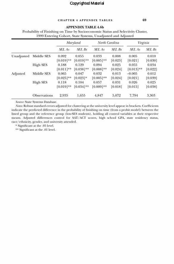
C H A P T E R 4 A P P E N D I X T A B L E S 69
APPENDIX TABLE 4.6bProbability of Finishing on Time by Socioeconomic Status and Selectivity Cluster,
1999 Entering Cohort, State Systems, Unadjusted and Adjusted
Maryland North Carolina Virginia
SEL As SEL Bs SEL As SEL Bs SEL As SEL Bs
Unadjusted Middle SES 0.092 0.055 0.033 0.008 0.005 0.010[0.019]** [0.019]** [0.005]** [0.023] [0.021] [0.030]
High SES 0.188 0.129 0.094 0.025 0.055 0.034[0.011]** [0.038]** [0.008]** [0.024] [0.013]** [0.022]
Adjusted Middle SES 0.065 0.047 0.032 0.013 –0.005 0.012[0.025]** [0.023]* [0.005]** [0.024] [0.021] [0.039]
High SES 0.118 0.104 0.057 0.031 0.026 0.025[0.019]** [0.034]** [0.009]** [0.018] [0.015] [0.038]
Observations 2,935 1,655 4,847 5,072 7,794 3,303
Source: State Systems Database.Notes: Robust standard errors adjusted for clustering at the university level appear in brackets. Coefficients
indicate the predicted difference in the probability of finishing on time (from a probit model) between thelisted group and the reference group (low-SES students), holding all control variables at their respectivemeans. Adjusted differences control for SAT/ACT scores, high school GPA, state residency status,race/ethnicity, gender, and university attended.
* Significant at the .05 level.** Significant at the .01 level.
Copyrighted MaterialCopyrighted MaterialCopyrighted Material

70 C H A P T E R 4 A P P E N D I X T A B L E S
APPENDIX TABLE 4.7aProbability of Finishing on Time by Parental Education and Selectivity Cluster,
1999 Entering Cohort, Flagships, Unadjusted and Adjusted
SEL Is SEL IIs SEL IIIs
Unadjusted Some College 0.084 0.020 –0.028[0.017]** [0.016] [0.024]
College Degree 0.149 0.076 0.006[0.016]** [0.021]** [0.032]
Graduate Degree 0.170 0.087 0.018[0.020]** [0.018]** [0.032]
Adjusted without Some College 0.029 –0.003 –0.029Family Income [0.009]** [0.012] [0.014]*
College Degree 0.052 0.050 0.019[0.009]** [0.016]** [0.011]
Graduate Degree 0.058 0.050 0.019[0.008]** [0.014]** [0.016]
Adjusted with Some College 0.018 –0.013 –0.030Family Income [0.008]* [0.011] [0.014]*
College Degree 0.031 0.028 0.016[0.009]** [0.014] [0.010]
Graduate Degree 0.030 0.020 0.015[0.009]** [0.011] [0.017]
Observations 17,279 13,760 10,588
Source: Flagships Database.Notes: Robust standard errors adjusted for clustering at the university level appear in
brackets. Coefficients indicate the predicted difference in the probability of finishing ontime (from a probit model) between the listed group and the reference group (studentswhose parents had no education beyond high school), holding all control variables at theirrespective means. Adjusted differences control for SAT/ACT scores, high school GPA, stateresidency status, race/ethnicity, gender, and university attended.
* Significant at the .05 level.** Significant at the .01 level.
Copyrighted MaterialCopyrighted MaterialCopyrighted Material

C H A P T E R 4 A P P E N D I X T A B L E S 71
APPENDIX TABLE 4.7bProbability of Finishing on Time by Parental Education and Selectivity Cluster, 1999 Entering
Cohort, State Systems, Unadjusted and Adjusted
Maryland North Carolina Virginia
SEL As SEL Bs SEL As SEL Bs SEL As SEL Bs
Unadjusted Some College 0.031 0.049 0.033 –0.015 0.004 0.045[0.043] [0.062] [0.032] [0.023] [0.022] [0.027]
College Degree 0.124 0.108 0.079 0.007 0.020 0.040[0.023]** [0.041]** [0.030]** [0.025] [0.020] [0.027]
Graduate Degree 0.162 0.123 0.130 0.043 0.053 0.067[0.014]** [0.057]* [0.018]** [0.026] [0.011]** [0.025]**
Adjusted Some College 0.014 0.038 0.002 –0.011 –0.014 0.051without [0.033] [0.081] [0.026] [0.020] [0.023] [0.028]Family College Degree 0.077 0.087 0.038 0.011 –0.005 0.042Income [0.008]** [0.059] [0.025] [0.022] [0.020] [0.034]
Graduate Degree 0.101 0.109 0.033 0.040 0.007 0.066[0.007]** [0.082] [0.026] [0.027] [0.020] [0.018]**
Adjusted Some College 0.007 0.035 –0.006 –0.011 –0.018 0.051with [0.032] [0.082] [0.020] [0.022] [0.021] [0.028]Family College Degree 0.055 0.077 0.025 0.012 –0.014 0.041Income [0.008]** [0.062] [0.017] [0.026] [0.021] [0.031]
Graduate Degree 0.073 0.090 0.016 0.040 –0.005 0.066[0.008]** [0.084] [0.014] [0.032] [0.023] [0.019]**
Observations 2,935 1,655 4,847 5,072 7,794 3,303
Source: State Systems Database.Notes: Robust standard errors adjusted for clustering at the university level appear in brackets. Coefficients
indicate the predicted difference in the probability of finishing on time (from a probit model) between thelisted group and the reference group (students whose parents had no education beyond high school), hold-ing all control variables at their respective means. Adjusted differences control for SAT/ACT scores, highschool GPA, state residency status, race/ethnicity, gender, and university attended.
* Significant at the .05 level.** Significant at the .01 level.
Copyrighted MaterialCopyrighted MaterialCopyrighted Material
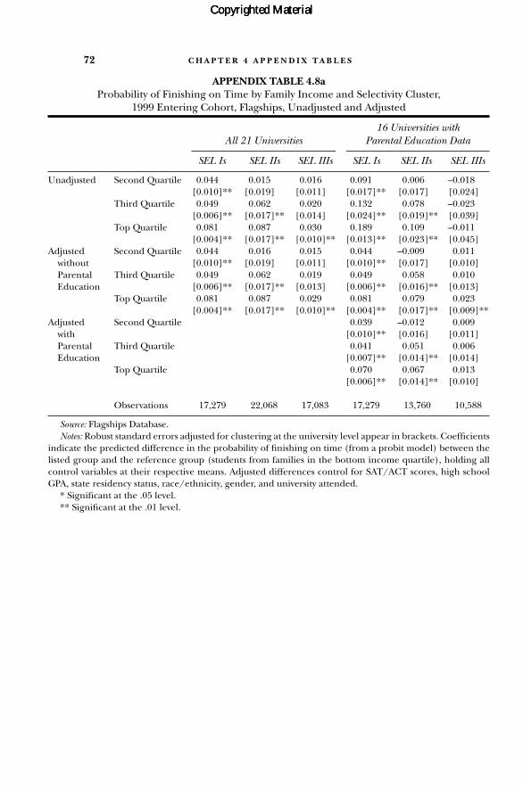
72 C H A P T E R 4 A P P E N D I X T A B L E S
APPENDIX TABLE 4.8aProbability of Finishing on Time by Family Income and Selectivity Cluster,
1999 Entering Cohort, Flagships, Unadjusted and Adjusted
16 Universities withAll 21 Universities Parental Education Data
SEL Is SEL IIs SEL IIIs SEL Is SEL IIs SEL IIIs
Unadjusted Second Quartile 0.044 0.015 0.016 0.091 0.006 –0.018[0.010]** [0.019] [0.011] [0.017]** [0.017] [0.024]
Third Quartile 0.049 0.062 0.020 0.132 0.078 –0.023[0.006]** [0.017]** [0.014] [0.024]** [0.019]** [0.039]
Top Quartile 0.081 0.087 0.030 0.189 0.109 –0.011[0.004]** [0.017]** [0.010]** [0.013]** [0.023]** [0.045]
Adjusted Second Quartile 0.044 0.016 0.015 0.044 –0.009 0.011without [0.010]** [0.019] [0.011] [0.010]** [0.017] [0.010]Parental Third Quartile 0.049 0.062 0.019 0.049 0.058 0.010Education [0.006]** [0.017]** [0.013] [0.006]** [0.016]** [0.013]
Top Quartile 0.081 0.087 0.029 0.081 0.079 0.023[0.004]** [0.017]** [0.010]** [0.004]** [0.017]** [0.009]**
Adjusted Second Quartile 0.039 –0.012 0.009with [0.010]** [0.016] [0.011]Parental Third Quartile 0.041 0.051 0.006Education [0.007]** [0.014]** [0.014]
Top Quartile 0.070 0.067 0.013[0.006]** [0.014]** [0.010]
Observations 17,279 22,068 17,083 17,279 13,760 10,588
Source: Flagships Database.Notes: Robust standard errors adjusted for clustering at the university level appear in brackets. Coefficients
indicate the predicted difference in the probability of finishing on time (from a probit model) between thelisted group and the reference group (students from families in the bottom income quartile), holding allcontrol variables at their respective means. Adjusted differences control for SAT/ACT scores, high schoolGPA, state residency status, race/ethnicity, gender, and university attended.
* Significant at the .05 level.** Significant at the .01 level.
Copyrighted MaterialCopyrighted MaterialCopyrighted Material

AP
PE
ND
IX T
AB
LE
4.8
bPr
obab
ility
of F
inis
hin
g on
Tim
e by
Fam
ily I
nco
me
and
Sele
ctiv
ity
Clu
ster
, 19
99 E
nte
rin
g C
ohor
t, St
ate
Syst
ems,
Un
adju
sted
an
d A
djus
ted
Mar
ylan
dN
orth
Car
olin
aO
hio
Virg
inia
SEL
As
SEL
Bs
SEL
As
SEL
Bs
SEL
As
SEL
Bs
SEL
As
SEL
Bs
Un
adju
sted
Seco
nd
Qua
rtile
0.07
60.
026
–0.0
02–0
.075
0.04
30.
027
0.00
90.
067
[0.0
18]*
*[0
.014
][0
.050
][0
.035
]*[0
.032
][0
.019
][0
.030
][0
.026
]*T
hir
d Q
uart
ile0.
130
0.07
00.
021
–0.0
460.
053
0.05
70.
046
0.05
7[0
.010
]**
[0.0
73]
[0.0
29]
[0.0
44]
[0.0
29]
[0.0
25]*
[0.0
23]*
[0.0
39]
Top
Qua
rtile
0.20
00.
132
0.05
6–0
.051
0.13
10.
109
0.07
10.
066
[0.0
05]*
*[0
.076
][0
.050
][0
.037
][0
.044
]**
[0.0
28]*
*[0
.017
]**
[0.0
25]*
*A
djus
ted
Seco
nd
Qua
rtile
0.05
40.
015
0.06
8–0
.056
–0.0
010.
019
0.00
20.
028
wit
hou
t [0
.022
]*[0
.028
][0
.040
][0
.027
]*[0
.006
][0
.020
][0
.033
][0
.028
]Pa
ren
tal
Th
ird
Qua
rtile
0.07
80.
046
0.07
0–0
.034
–0.0
130.
050
0.03
70.
027
Edu
cati
on[0
.016
]**
[0.0
50]
[0.0
15]*
*[0
.030
][0
.014
][0
.018
]**
[0.0
31]
[0.0
43]
Top
Qua
rtile
0.12
10.
097
0.08
7–0
.027
0.03
20.
086
0.04
40.
026
[0.0
14]*
*[0
.015
]**
[0.0
40]*
[0.0
25]
[0.0
11]*
*[0
.017
]**
[0.0
31]
[0.0
37]
Adj
uste
d Se
con
d Q
uart
ile0.
046
0.00
50.
067
–0.0
560.
003
0.02
6w
ith
[0
.020
]*[0
.032
][0
.037
][0
.027
]*[0
.033
][0
.028
]Pa
ren
tal
Th
ird
Qua
rtile
0.05
90.
026
0.06
6–0
.036
0.03
80.
019
Edu
cati
on[0
.014
]**
[0.0
54]
[0.0
13]*
*[0
.030
][0
.031
][0
.041
]To
p Q
uart
ile0.
093
0.06
50.
080
–0.0
380.
044
0.01
4[0
.009
]**
[0.0
07]*
*[0
.038
]*[0
.027
][0
.032
][0
.035
]
Obs
erva
tion
s2,
935
1,65
54,
847
5,07
24,
902
8,35
37,
794
3,30
3
Sour
ce:S
tate
Sys
tem
s D
atab
ase.
Not
es:R
obus
t sta
nda
rd e
rror
s ad
just
ed fo
r cl
uste
rin
g at
the
univ
ersi
ty le
vel a
ppea
r in
bra
cket
s. C
oeffi
cien
ts in
dica
te th
e pr
edic
ted
diff
eren
ce in
the
prob
abili
ty o
f fi
nis
hin
g on
tim
e (f
rom
a p
robi
t m
odel
) be
twee
n t
he
liste
d gr
oup
and
the
refe
ren
ce g
roup
(st
uden
ts f
rom
fam
ilies
in t
he
bott
om in
-co
me
quar
tile
), h
oldi
ng
all c
ontr
ol v
aria
bles
at t
hei
r re
spec
tive
mea
ns.
Adj
uste
d di
ffer
ence
s co
ntr
ol fo
r SA
T/A
CT
sco
res,
hig
h s
choo
l GPA
, sta
te r
esi-
den
cy s
tatu
s, r
ace/
eth
nic
ity,
gen
der,
and
univ
ersi
ty a
tten
ded.
* Si
gnifi
can
t at t
he
.05
leve
l.**
Sig
nifi
can
t at t
he
.01
leve
l.
Copyrighted MaterialCopyrighted MaterialCopyrighted Material
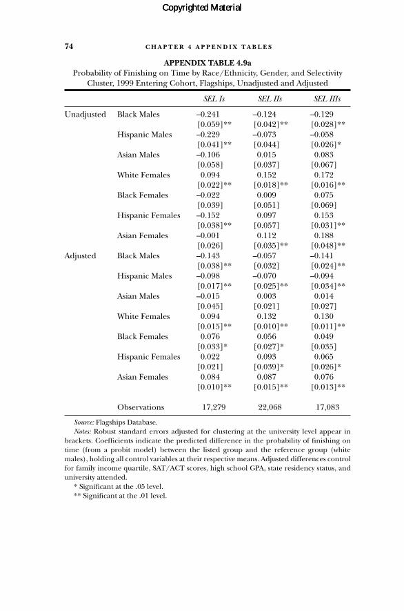
74 C H A P T E R 4 A P P E N D I X T A B L E S
APPENDIX TABLE 4.9aProbability of Finishing on Time by Race/Ethnicity, Gender, and Selectivity
Cluster, 1999 Entering Cohort, Flagships, Unadjusted and Adjusted
SEL Is SEL IIs SEL IIIs
Unadjusted Black Males –0.241 –0.124 –0.129[0.059]** [0.042]** [0.028]**
Hispanic Males –0.229 –0.073 –0.058[0.041]** [0.044] [0.026]*
Asian Males –0.106 0.015 0.083[0.058] [0.037] [0.067]
White Females 0.094 0.152 0.172[0.022]** [0.018]** [0.016]**
Black Females –0.022 0.009 0.075[0.039] [0.051] [0.069]
Hispanic Females –0.152 0.097 0.153[0.038]** [0.057] [0.031]**
Asian Females –0.001 0.112 0.188[0.026] [0.035]** [0.048]**
Adjusted Black Males –0.143 –0.057 –0.141[0.038]** [0.032] [0.024]**
Hispanic Males –0.098 –0.070 –0.094[0.017]** [0.025]** [0.034]**
Asian Males –0.015 0.003 0.014[0.045] [0.021] [0.027]
White Females 0.094 0.132 0.130[0.015]** [0.010]** [0.011]**
Black Females 0.076 0.056 0.049[0.033]* [0.027]* [0.035]
Hispanic Females 0.022 0.093 0.065[0.021] [0.039]* [0.026]*
Asian Females 0.084 0.087 0.076[0.010]** [0.015]** [0.013]**
Observations 17,279 22,068 17,083
Source: Flagships Database.Notes: Robust standard errors adjusted for clustering at the university level appear in
brackets. Coefficients indicate the predicted difference in the probability of finishing ontime (from a probit model) between the listed group and the reference group (whitemales), holding all control variables at their respective means. Adjusted differences controlfor family income quartile, SAT/ACT scores, high school GPA, state residency status, anduniversity attended.
* Significant at the .05 level.** Significant at the .01 level.
Copyrighted MaterialCopyrighted MaterialCopyrighted Material
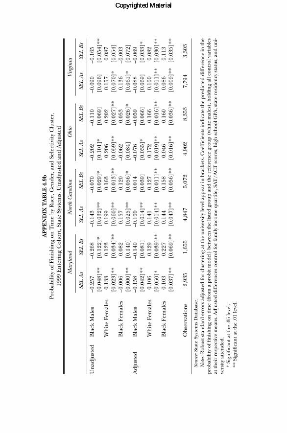
AP
PE
ND
IX T
AB
LE
4.9
bPr
obab
ility
of F
inis
hin
g on
Tim
e by
Rac
e, G
ende
r, an
d Se
lect
ivit
y C
lust
er,
1999
En
teri
ng
Coh
ort,
Stat
e Sy
stem
s, U
nad
just
ed a
nd
Adj
uste
d
Mar
ylan
dN
orth
Car
olin
aO
hio
Virg
inia
SEL
As
SEL
Bs
SEL
As
SEL
Bs
SEL
As
SEL
Bs
SEL
As
SEL
Bs
Un
adju
sted
Bla
ck M
ales
–0.2
57–0
.268
–0.1
43–0
.070
–0.2
02–0
.110
–0.0
90–0
.165
[0.0
48]*
*[0
.122
]*[0
.032
]**
[0.0
29]*
[0.1
01]*
[0.0
69]
[0.0
96]
[0.0
54]*
*W
hit
e Fe
mal
es0.
133
0.12
30.
199
0.16
30.
206
0.20
20.
157
0.08
7[0
.023
]**
[0.0
34]*
*[0
.060
]**
[0.0
13]*
*[0
.059
]**
[0.0
27]*
*[0
.070
]*[0
.054
]B
lack
Fem
ales
–0.0
060.
082
0.15
70.
120
–0.0
620.
053
0.13
6–0
.003
[0.0
00]*
*[0
.140
][0
.025
]**
[0.0
56]*
[0.0
84]
[0.0
26]*
[0.0
61]*
[0.0
72]
Adj
uste
dB
lack
Mal
es–0
.158
–0.1
40–0
.100
0.01
4–0
.076
–0.0
59–0
.088
–0.0
69[0
.042
]**
[0.0
81]
[0.0
14]*
*[0
.039
][0
.035
]*[0
.066
][0
.069
][0
.033
]*W
hit
e Fe
mal
es0.
106
0.12
90.
141
0.12
70.
172
0.16
60.
100
0.08
2[0
.050
]*[0
.039
]**
[0.0
14]*
*[0
.011
]**
[0.0
19]*
*[0
.016
]**
[0.0
11]*
*[0
.030
]**
Bla
ck F
emal
es0.
103
0.22
70.
144
0.15
80.
046
0.16
00.
086
0.11
3[0
.037
]**
[0.0
69]*
*[0
.047
]**
[0.0
56]*
*[0
.016
]**
[0.0
36]*
*[0
.009
]**
[0.0
35]*
*
Obs
erva
tion
s2,
935
1,65
54,
847
5,07
24,
902
8,35
37,
794
3,30
3
Sour
ce:S
tate
Sys
tem
s D
atab
ase.
Not
es:R
obus
t sta
nda
rd e
rror
s ad
just
ed fo
r cl
uste
rin
g at
the
univ
ersi
ty le
vel a
ppea
r in
bra
cket
s. C
oeffi
cien
ts in
dica
te th
e pr
edic
ted
diff
eren
ce in
the
prob
abili
ty o
f fin
ish
ing
on ti
me
(fro
m a
pro
bit m
odel
) be
twee
n th
e lis
ted
grou
p an
d th
e re
fere
nce
gro
up (
wh
ite
mal
es),
hol
din
g al
l con
trol
var
iabl
esat
thei
r re
spec
tive
mea
ns.
Adj
uste
d di
ffer
ence
s co
ntr
ol fo
r fa
mily
inco
me
quar
tile
, SA
T/A
CT
sco
res,
hig
h s
choo
l GPA
, sta
te r
esid
ency
sta
tus,
an
d un
i-ve
rsit
y at
ten
ded.
* Si
gnifi
can
t at t
he
.05
leve
l.**
Sig
nifi
can
t at t
he
.01
leve
l.
Copyrighted MaterialCopyrighted MaterialCopyrighted Material

76 C H A P T E R 4 A P P E N D I X T A B L E S
APPENDIX TABLE 4.10aRank-in-Class at Graduation by Socioeconomic Status and Selectivity Cluster,
1999 Entering Cohort, Flagships, Unadjusted and Adjusted
SEL Is SEL IIs SEL IIIs
Unadjusted Middle SES 6.3 4.9 3.3[1.0]** [0.7]* [0.9]*
High SES 12.6 9.0 7.5[0.8]** [1.7]* [1.5]**
Adjusted Middle SES –0.9 0.6 –0.4[0.8] [0.1]* [0.9]
High SES 1.1 3.3 1.7[1.1] [0.4]* [0.9]
Observations 17,170 8,550 10,626
Source: Flagships Database.Notes: Robust standard errors adjusted for clustering at the university level appear in
brackets. Coefficients indicate the predicted difference in rank-in-class (in percentilepoints) relative to the reference group (low-SES students). Adjusted differences control forSAT/ACT scores, high school GPA, state residency status, race/ethnicity, gender, major, anduniversity attended.
* Significant at the .05 level.** Significant at the .01 level.
Copyrighted MaterialCopyrighted MaterialCopyrighted Material

C H A P T E R 4 A P P E N D I X T A B L E S 77
APPENDIX TABLE 4.10bRank-in-Class at Graduation by Socioeconomic Status and Selectivity Cluster,
1999 Entering Cohort, State Systems, Unadjusted and Adjusted
Maryland North Carolina Virginia
SEL As SEL Bs SEL As SEL Bs SEL As SEL Bs
Unadjusted Middle SES 6.0 –0.2 6.8 3.9 2.7 0.5[2.7] [3.5] [2.2] [1.7] [1.7] [1.5]
High SES 10.5 –1.3 13.0 4.2 8.1 1.9[4.0] [2.3] [3.7] [2.1] [1.8]* [2.2]
Adjusted Middle SES 2.4 –0.5 0.5 2.5 0.2 –0.4[0.5] [2.5] [1.5] [1.1] [1.2] [0.7]
High SES 4.5 1.0 2.1 2.8 3.6 –0.4[1.4] [1.5] [0.8] [1.3] [1.3] [0.7]
Observations 2,936 1,656 4,847 5,072 7,872 3,428
Source: State Systems Database.Notes: Robust standard errors adjusted for clustering at the university level appear in brackets. Coefficients
indicate the predicted difference in rank-in-class (in percentile points) relative to the reference group (low-SES students). Adjusted differences control for SAT/ACT scores, high school GPA, state residency status,race/ethnicity, gender, major, and university attended.
* Significant at the .05 level.** Significant at the .01 level.
Copyrighted MaterialCopyrighted MaterialCopyrighted Material

78 C H A P T E R 4 A P P E N D I X T A B L E S
APPENDIX TABLE 4.11aRank-in-Class at Graduation by Parental Education and Selectivity Cluster,
1999 Entering Cohort, Flagships, Unadjusted and Adjusted
SEL Is SEL IIs SEL IIIs
Unadjusted Some College 2.8 –0.6 0.7[0.5]** [2.2] [1.3]
College Degree 8.5 5.3 5.2[0.6]** [0.4]** [1.2]*
Graduate Degree 13.4 6.0 8.2[1.0]** [0.8]* [2.2]*
Adjusted Some College –2.6 –0.8 –0.8without [0.5]** [2.0] [1.3]Family College Degree –0.9 2.7 0.7Income [1.0] [0.9] [0.9]
Graduate Degree 2.0 2.6 2.8[0.9] [0.2]** [1.5]
Adjusted Some College –2.3 –0.9 –0.7with [0.5]** [2.0] [1.2]Family College Degree –0.6 2.3 0.7Income [0.7] [0.7] [0.7]
Graduate Degree 2.0 1.9 2.7[0.6]* [0.4]* [1.4]
Observations 17,170 8,550 10,626
Source: Flagships Database.Notes: Robust standard errors adjusted for clustering at the university level appear in
brackets. Coefficients indicate the predicted difference in rank-in-class (in percentile points)relative to the reference group (no college). Adjusted differences control for SAT/ACTscores, high school GPA, state residency status, race/ethnicity, gender, major, and univer-sity attended.
* Significant at the .05 level.** Significant at the .01 level.
Copyrighted MaterialCopyrighted MaterialCopyrighted Material

C H A P T E R 4 A P P E N D I X T A B L E S 79
APPENDIX TABLE 4.11bRank-in-Class at Graduation by Parental Education and Selectivity Cluster, 1999 Entering
Cohort, State Systems, Unadjusted and Adjusted
Maryland North Carolina Virginia
SEL As SEL Bs SEL As SEL Bs SEL As SEL Bs
Unadjusted Some College –0.5 5.1 3.0 0.3 –1.1 0.4[3.3] [1.4] [0.6]* [1.0] [1.8] [1.5]
College Degree 4.8 2.4 8.7 2.7 3.9 0.8[3.5] [2.3] [2.9] [1.4] [1.4]* [2.3]
Graduate Degree 7.8 3.1 14.2 5.7 7.2 3.4[4.2] [0.5]* [3.0]* [1.5]** [2.9] [2.4]
Adjusted Some College –1.5 2.5 –1.3 –0.7 –2.9 –0.2without [2.1] [2.3] [1.2] [0.8] [1.2] [1.0]Family College Degree 1.9 0.5 0.9 1.1 0.7 –0.2Income [1.7] [2.1] [0.9] [1.0] [0.6] [1.7]
Graduate Degree 3.4 2.5 2.9 3.2 3.2 0.3[1.8] [0.9] [0.7] [1.2]* [1.1]* [1.3]
Adjusted Some College –1.5 2.4 –1.3 –0.7 –2.9 –0.1 with [2.0] [2.4] [1.2] [0.7] [1.2] [1.0]Family College Degree 1.6 0.2 0.8 1.2 0.4 0.0Income [1.3] [2.1] [1.0] [1.1] [0.4] [1.8]
Graduate Degree 3.1 2.0 2.6 3.3 2.7 0.6[1.2] [2.0] [0.9] [1.2]* [1.0] [1.5]
Observations 2,936 1,656 4,847 5,072 7,872 3,428
Source: State Systems Database.Notes: Robust standard errors adjusted for clustering at the university level appear in brackets. Coefficients
indicate the predicted difference in rank-in-class (in percentile points) relative to the reference group (nocollege). Adjusted differences control for SAT/ACT scores, high school GPA, state residency status,race/ethnicity, gender, major, and university attended.
* Significant at the .05 level.** Significant at the .01 level.
Copyrighted MaterialCopyrighted MaterialCopyrighted Material

80 C H A P T E R 4 A P P E N D I X T A B L E S
APPENDIX TABLE 4.12aRank-in-Class at Graduation by Family Income and Selectivity Cluster,
1999 Entering Cohort, Flagships, Unadjusted and Adjusted
14 Universities with19 Universities Parental Education Data
SEL Is SEL IIs SEL IIIs SEL Is SEL IIs SEL IIIs
Unadjusted Second Quartile 2.3 3.8 1.2 2.3 2.2 0.3[1.1] [1.0]* [1.3] [1.1] [0.3]* [1.5]
Third Quartile 4.7 6.1 2.4 4.7 5.3 2.7[0.8]** [0.7]** [1.2] [0.8]** [0.9]* [1.5]
Top Quartile 10.4 8.9 4.5 10.4 7.6 4.5[1.0]** [1.2]** [1.5]* [1.0]** [1.0]* [1.6]
Adjusted Second Quartile –1.7 –0.1 –1.2 –1.7 –1.4 –2.4without [1.0] [1.0] [1.2] [1.0] [1.2] [1.3]Parental Third Quartile –2.5 –0.1 –1.5 –2.5 –0.3 –1.6Education [1.0] [0.5] [0.8] [1.0] [1.0] [1.1]
Top Quartile 0.2 2.0 0.4 0.2 1.6 –0.2[0.9] [0.6]* [1.0] [0.9] [0.8] [1.4]
Adjusted Second Quartile –1.7 –1.6 –2.5with [1.0] [1.3] [1.3]Parental Third Quartile –2.8 –0.8 –2.0Education [0.9]* [1.0] [1.1]
Top Quartile –0.8 0.6 –1.1[0.7] [1.3] [1.3]
Observations 17,170 16,858 17,121 17,170 8,550 10,626
Source: Flagships Database.Notes: Robust standard errors adjusted for clustering at the university level appear in brackets. Coefficients
indicate the predicted difference in rank-in-class (in percentile points) relative to the reference group (bot-tom quartile). Adjusted differences control for SAT/ACT scores, high school GPA, state residency status,race/ethnicity, gender, major, and university attended.
* Significant at the .05 level.** Significant at the .01 level.
Copyrighted MaterialCopyrighted MaterialCopyrighted Material
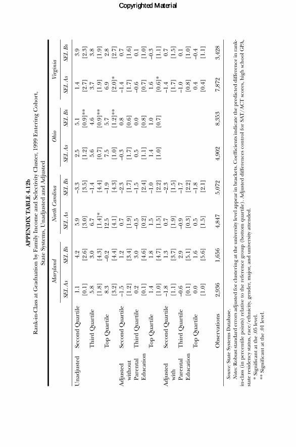
AP
PE
ND
IX T
AB
LE
4.1
2bR
ank-
in-C
lass
at G
radu
atio
n b
y Fa
mily
In
com
e an
d Se
lect
ivit
y C
lust
er, 1
999
En
teri
ng
Coh
ort,
Stat
e Sy
stem
s, U
nad
just
ed a
nd
Adj
uste
d
Mar
ylan
dN
orth
Car
olin
aO
hio
Virg
inia
SEL
As
SEL
Bs
SEL
As
SEL
Bs
SEL
As
SEL
Bs
SEL
As
SEL
Bs
Un
adju
sted
Seco
nd
Qua
rtile
1.1
4.2
5.9
–3.3
2.5
5.1
1.4
3.9
[0.1
][2
.6]
[3.0
][3
.5]
[1.2
][0
.9]*
*[2
.7]
[2.3
]T
hir
d Q
uart
ile5.
83.
06.
7–1
.45.
64.
63.
73.
8[1
.8]
[4.3
][1
.4]*
[4.4
][0
.7]
[0.9
]**
[1.9
][1
.9]
Top
Qua
rtile
8.3
–0.2
12.5
–1.9
7.5
5.7
6.9
2.8
[3.2
][4
.4]
[4.1
][4
.3]
[1.0
][1
.2]*
*[2
.0]*
[2.7
]A
djus
ted
Seco
nd
Qua
rtile
–1.5
1.2
0.7
–2.3
–0.3
0.8
–1.4
0.7
wit
hou
t [1
.2]
[3.4
][1
.9]
[1.7
][1
.7]
[0.6
][1
.7]
[1.6
]Pa
ren
tal
Th
ird
Qua
rtile
0.2
3.0
–0.5
–1.5
0.5
0.0
–0.6
0.1
Edu
cati
on[0
.1]
[4.6
][0
.2]
[2.4
][1
.1]
[0.8
][0
.7]
[1.0
]To
p Q
uart
ile1.
41.
81.
5–1
.01.
41.
01.
6–0
.3[1
.0]
[4.7
][1
.5]
[2.2
][1
.0]
[0.7
][0
.6]*
[1.1
]A
djus
ted
Seco
nd
Qua
rtile
–1.8
1.3
0.7
–2.3
–1.4
0.7
wit
h
[1.1
][3
.7]
[1.9
][1
.5]
[1.7
][1
.5]
Pare
nta
l T
hir
d Q
uart
ile–0
.62.
9–0
.9–1
.7–1
.00.
1E
duca
tion
[0.1
][5
.1]
[0.3
][2
.2]
[0.8
][1
.0]
Top
Qua
rtile
0.0
1.6
0.5
–1.8
0.4
–0.4
[1.0
][5
.6]
[1.5
][2
.1]
[0.4
][1
.1]
Obs
erva
tion
s2,
936
1,65
64,
847
5,07
24,
902
8,35
37,
872
3,42
8
Sour
ce:S
tate
Sys
tem
s D
atab
ase.
Not
es:R
obus
t sta
nda
rd e
rror
s adj
uste
d fo
r cl
uste
rin
g at
the
univ
ersi
ty le
vel a
ppea
r in
bra
cket
s. C
oeffi
cien
ts in
dica
te th
e pr
edic
ted
diff
eren
ce in
ran
k-in
-cla
ss (
in p
erce
nti
le p
oin
ts)
rela
tive
to
the
refe
ren
ce g
roup
(bo
ttom
qua
rtile
). A
djus
ted
diff
eren
ces
con
trol
for
SA
T/A
CT
sco
res,
hig
h s
choo
l GPA
,st
ate
resi
den
cy s
tatu
s, r
ace/
eth
nic
ity,
gen
der,
maj
or, a
nd
univ
ersi
ty a
tten
ded.
* Si
gnifi
can
t at t
he
.05
leve
l.**
Sig
nifi
can
t at t
he
.01
leve
l.
Copyrighted MaterialCopyrighted MaterialCopyrighted Material
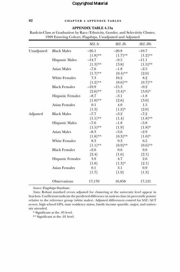
82 C H A P T E R 4 A P P E N D I X T A B L E S
APPENDIX TABLE 4.13aRank-in-Class at Graduation by Race/Ethnicity, Gender, and Selectivity Cluster,
1999 Entering Cohort, Flagships, Unadjusted and Adjusted
SEL Is SEL IIs SEL IIIs
Unadjusted Black Males –26.1 –20.8 –19.7[1.8]** [1.7]** [1.2]**
Hispanic Males –14.7 –9.5 –11.1[1.3]** [3.8] [1.5]**
Asian Males –7.6 –1.8 –2.5[1.7]** [0.4]** [2.0]
White Females 7.3 10.2 8.2[1.2]** [0.6]** [0.7]**
Black Females –19.9 –15.3 –9.2[2.6]** [3.4]* [3.0]*
Hispanic Females –8.7 –3.1 –1.8[1.0]** [2.6] [3.0]
Asian Females 0.1 4.0 1.5[1.3] [1.2]* [2.0]
Adjusted Black Males –7.7 –3.2 –7.2[1.1]** [1.4] [1.8]**
Hispanic Males –7.6 –1.8 –5.8[1.5]** [1.9] [1.8]*
Asian Males –8.3 –3.6 –2.9[1.8]** [0.3]** [1.0]*
White Females 8.3 9.3 6.5[1.1]** [0.9]** [0.6]**
Black Females –2.6 0.6 0.0[2.4] [1.6] [2.1]
Hispanic Females 3.9 4.7 2.6[1.8] [1.3]* [2.1]
Asian Females 0.1 3.1 0.9[1.7] [1.9] [1.3]
Observations 17,170 16,858 17,121
Source: Flagships Database.Notes: Robust standard errors adjusted for clustering at the university level appear in
brackets. Coefficients indicate the predicted difference in rank-in-class (in percentile points)relative to the reference group (white males). Adjusted differences control for SAT/ACTscores, high school GPA, state residency status, family income quartile, major, and univer-sity attended.
* Significant at the .05 level.** Significant at the .01 level.
Copyrighted MaterialCopyrighted MaterialCopyrighted Material

AP
PE
ND
IX T
AB
LE
4.1
3bR
ank-
in-C
lass
at G
radu
atio
n b
y R
ace,
Gen
der,
and
Sele
ctiv
ity
Clu
ster
, 199
9 E
nte
rin
g C
ohor
t, St
ate
Syst
ems,
Un
adju
sted
an
d A
djus
ted
Mar
ylan
dN
orth
Car
olin
aO
hio
Virg
inia
SEL
As
SEL
Bs
SEL
As
SEL
Bs
SEL
As
SEL
Bs
SEL
As
SEL
Bs
Un
adju
sted
Bla
ck M
ales
–21.
5–1
5.4
–23.
9–1
4.0
–22.
5–2
1.0
–20.
9–1
3.2
[3.4
][3
.9]
[6.6
][2
.3]*
*[1
.9]
[1.7
]**
[0.9
]**
[2.4
]**
Wh
ite
Fem
ales
11.4
14.4
6.2
13.9
9.5
11.2
8.9
9.0
[2.4
][1
.1]*
*[1
.1]*
[0.7
]**
[4.3
][1
.4]*
*[2
.2]*
[1.5
]**
Bla
ck F
emal
es–7
.5–2
.0–1
7.9
–2.5
–14.
3–1
0.5
–16.
9–6
.0[2
.5]
[4.5
][4
.3]
[2.9
][1
.2]
[2.2
]**
[3.0
]**
[4.3
]A
djus
ted
Bla
ck M
ales
–7.2
–5.2
–5.0
–3.7
–4.6
–9.1
–4.3
–8.1
[0.9
][3
.2]
[1.5
][0
.7]*
*[0
.7]
[1.4
]**
[1.2
]*[1
.5]*
*W
hit
e Fe
mal
es10
.811
.48.
69.
09.
57.
38.
44.
7[3
.8]
[1.6
]*[1
.0]*
[0.5
]**
[2.9
][1
.4]*
*[1
.1]*
*[0
.8]*
*B
lack
Fem
ales
5.1
6.3
–0.3
2.8
1.6
–0.8
–0.3
–2.8
[2.6
][6
.2]
[0.9
][3
.0]
[3.0
][1
.6]
[1.7
][1
.9]
Obs
erva
tion
s2,
936
1,65
64,
847
5,07
24,
902
8,35
37,
872
3,42
8
Sour
ce:S
tate
Sys
tem
s D
atab
ase.
Not
es:R
obus
t sta
nda
rd e
rror
s adj
uste
d fo
r cl
uste
rin
g at
the
univ
ersi
ty le
vel a
ppea
r in
bra
cket
s. C
oeffi
cien
ts in
dica
te th
e pr
edic
ted
diff
eren
ce in
ran
k-in
-cla
ss (
in p
erce
nti
le p
oin
ts)
rela
tive
to th
e re
fere
nce
gro
up (
wh
ite
mal
es).
Adj
uste
d di
ffer
ence
s co
ntr
ol fo
r SA
T/A
CT
sco
res,
hig
h s
choo
l GPA
, sta
tere
side
ncy
sta
tus,
fam
ily in
com
e qu
arti
le, m
ajor
, an
d un
iver
sity
att
ende
d.*
Sign
ifica
nt a
t th
e .0
5 le
vel.
** S
ign
ifica
nt a
t th
e .0
1 le
vel.
Copyrighted MaterialCopyrighted MaterialCopyrighted Material

AP
PE
ND
IX T
AB
LE
4.1
4aPr
edic
tin
g R
ank-
in-C
lass
at G
radu
atio
n b
y R
ace/
Eth
nic
ity,
Gen
der,
and
Sele
ctiv
ity
Clu
ster
, 199
9 E
nte
rin
g C
ohor
t, Fl
agsh
ips
SEL
Is
SEL
IIs
SEL
III
s
Bla
ck M
ales
–26.
1–2
3.9
–12.
0–1
5.3
–7.7
–20.
8–1
9.4
–8.9
–8.2
–3.2
–19.
7–1
8.3
–8.1
–11.
3–7
.2[1
.8]*
*[1
.8]*
*[1
.6]*
*[1
.1]*
*[1
.1]*
*[1
.7]*
*[1
.6]*
*[1
.0]*
*[1
.9]*
[1.4
][1
.2]*
*[1
.4]*
*[2
.2]*
*[1
.4]*
*[1
.8]*
*H
ispa
nic
Mal
es–1
4.7
–14.
0–8
.0–1
2.0
–7.6
–9.5
–8.6
–3.4
–4.6
–1.8
–11.
1–1
0.9
–5.8
–7.9
–5.8
[1.3
]**
[1.6
]**
[2.3
]*[1
.1]*
*[1
.5]*
*[3
.8]
[3.7
][2
.5]
[2.7
][1
.9]
[1.5
]**
[2.1
]**
[2.6
][1
.5]*
*[1
.8]*
Asi
an M
ales
–7.6
–7.6
–8.1
–8.1
–8.3
–1.8
–1.9
–2.8
–3.4
–3.6
–2.5
–4.6
–3.6
–3.6
–2.9
[1.7
]**
[1.9
]**
[1.8
]**
[1.8
]**
[1.8
]**
[0.4
]**
[0.8
][0
.6]*
*[0
.6]*
*[0
.3]*
*[2
.0]
[2.9
][2
.3]
[0.9
]**
[1.0
]*W
hit
e Fe
mal
es7.
37.
610
.35.
98.
310
.210
.012
.27.
59.
38.
29.
310
.84.
76.
5[1
.2]*
*[1
.2]*
*[1
.2]*
*[1
.0]*
*[1
.1]*
*[0
.6]*
*[0
.9]*
*[0
.7]*
*[1
.2]*
*[0
.9]*
*[0
.7]*
*[0
.7]*
*[0
.5]*
*[0
.5]*
*[0
.6]*
*B
lack
Fem
ales
–19.
9–1
7.3
–4.2
–11.
7–2
.6–1
5.3
–13.
4–0
.9–6
.50.
6–9
.2–7
.13.
9–5
.80.
0[2
.6]*
*[2
.7]*
*[2
.9]
[2.3
]**
[2.4
][3
.4]*
[3.1
]*[1
.9]
[2.5
][1
.6]
[3.0
]*[2
.0]*
*[1
.3]*
[2.7
][2
.1]
His
pan
ic F
emal
es–8
.7–7
.34.
1–4
.63.
9–3
.1–2
.35.
6–0
.34.
7–1
.8–0
.17.
2–1
.82.
6[1
.0]*
*[1
.8]*
*[2
.4]
[1.4
]*[1
.8]
[2.6
][2
.8]
[1.7
]*[2
.1]
[1.3
]*[3
.0]
[2.3
][1
.8]*
*[2
.0]
[2.1
]A
sian
Fem
ales
0.1
–0.3
1.9
–2.1
0.1
4.0
3.5
6.0
0.7
3.1
1.5
1.6
5.4
–2.5
0.9
[1.3
][1
.9]
[2.0
][1
.5]
[1.7
][1
.2]*
[1.9
][2
.1]*
[1.9
][1
.9]
[2.0
][1
.6]
[1.0
]**
[1.5
][1
.3]
Stan
dard
Con
trol
s?N
oYe
sYe
sYe
sYe
sN
oYe
sYe
sYe
sYe
sN
oYe
sYe
sYe
sYe
sSA
T/A
CT
Sco
res?
No
No
Yes
No
Yes
No
No
Yes
No
Yes
No
No
Yes
No
Yes
Hig
h S
choo
l GPA
?N
oN
oN
oYe
sYe
sN
oN
oN
oYe
sYe
sN
oN
oN
oYe
sYe
s
Obs
erva
tion
s17
,170
17,1
7017
,170
17,1
7017
,170
16,8
5816
,858
16,8
5816
,858
16,8
5817
,121
17,1
2117
,121
17,1
2117
,121
R-s
quar
ed0.
080.
110.
220.
200.
270.
060.
080.
170.
200.
240.
040.
060.
220.
260.
31
Sour
ce:F
lags
hip
s D
atab
ase.
Not
es:R
obus
t sta
nda
rd e
rror
s adj
uste
d fo
r cl
uste
rin
g at
the
univ
ersi
ty le
vel a
ppea
r in
bra
cket
s. C
oeffi
cien
ts in
dica
te th
e pr
edic
ted
diff
eren
ce in
ran
k-in
-cla
ss (
in p
erce
nti
lepo
ints
) re
lati
ve to
the
refe
ren
ce g
roup
(w
hit
e m
ales
). S
tan
dard
con
trol
s in
clud
e st
ate
resi
den
cy s
tatu
s, fa
mily
inco
me
quar
tile
, maj
or, a
nd
univ
ersi
ty a
tten
ded.
* Si
gnifi
can
t at t
he
.05
leve
l.**
Sig
nifi
can
t at t
he
.01
leve
l.
Copyrighted MaterialCopyrighted MaterialCopyrighted Material

AP
PE
ND
IX T
AB
LE
4.1
4bPr
edic
tin
g R
ank-
in-C
lass
at G
radu
atio
n b
y R
ace,
Gen
der,
and
Sele
ctiv
ity
Clu
ster
, 199
9 E
nte
rin
g C
ohor
t, St
ate
Syst
ems
SEL
As
SEL
Bs
Bla
ck M
ales
–22.
0–2
0.3
–8.4
–11.
4–4
.9–1
5.7
–15.
6–6
.9–1
0.4
–6.7
[1.7
]**
[1.5
]**
[0.9
]**
[1.0
]**
[0.5
]**
[1.3
]**
[1.2
]**
[0.8
]**
[1.0
]**
[0.9
]**
Wh
ite
Fem
ales
8.6
10.3
12.8
6.8
9.3
11.9
11.2
13.0
5.8
7.9
[1.3
]**
[1.1
]**
[1.1
]**
[0.9
]**
[0.9
]**
[0.8
]**
[0.7
]**
[0.7
]**
[0.7
]**
[0.7
]**
Bla
ck F
emal
es–1
4.3
–11.
52.
1–6
.91.
7–5
.2–5
.46.
1–6
.10.
5[2
.3]*
*[2
.0]*
*[1
.6]
[1.7
]**
[1.4
][1
.7]*
*[1
.7]*
*[1
.4]*
*[1
.4]*
*[1
.4]
Stan
dard
Con
trol
s?N
oYe
sYe
sYe
sYe
sN
oYe
sYe
sYe
sYe
sSA
T/A
CT
Sco
res?
No
No
Yes
No
Yes
No
No
Yes
No
Yes
Hig
h S
choo
l GPA
?N
oN
oN
oYe
sYe
sN
oN
oN
oYe
sYe
s
Obs
erva
tion
s20
,557
20,5
5720
,557
20,5
5720
,557
18,5
0918
,509
18,5
0918
,509
18,5
09
R-s
quar
ed0.
060.
080.
210.
220.
280.
060.
090.
240.
300.
34
Sour
ce:S
tate
Sys
tem
s D
atab
ase.
Not
es:R
obus
t st
anda
rd e
rror
s ad
just
ed f
or c
lust
erin
g at
th
e un
iver
sity
leve
l app
ear
in b
rack
ets.
Coe
ffici
ents
indi
cate
th
e pr
edic
ted
diff
eren
ce in
ran
k-in
-cl
ass
(in
per
cen
tile
poi
nts
) re
lati
ve to
the
refe
ren
ce g
roup
(w
hit
e m
ales
). S
tan
dard
con
trol
s in
clud
e st
ate
resi
den
cy s
tatu
s, fa
mily
inco
me
quar
tile
, maj
or, a
nd
univ
ersi
ty a
tten
ded.
* Si
gnifi
can
t at t
he
.05
leve
l.**
Sig
nifi
can
t at t
he
.01
leve
l.
Copyrighted MaterialCopyrighted MaterialCopyrighted Material
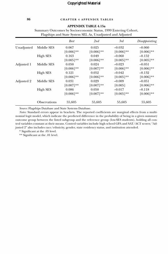
86 C H A P T E R 4 A P P E N D I X T A B L E S
APPENDIX TABLE 4.15aSummary Outcomes by Socioeconomic Status, 1999 Entering Cohort,
Flagships and State System SEL As, Unadjusted and Adjusted
Best 2nd 3rd Disappointing
Unadjusted Middle SES 0.067 0.025 –0.032 –0.060[0.006]** [0.006]** [0.006]** [0.006]**
High SES 0.163 0.049 –0.060 –0.152[0.005]** [0.006]** [0.005]** [0.005]**
Adjusted 1 Middle SES 0.050 0.024 –0.023 –0.051[0.006]** [0.007]** [0.006]** [0.006]**
High SES 0.121 0.052 –0.042 –0.132[0.006]** [0.006]** [0.005]** [0.006]**
Adjusted 2 Middle SES 0.031 0.029 –0.009 –0.051[0.007]** [0.007]** [0.005] [0.006]**
High SES 0.086 0.050 –0.017 –0.118[0.006]** [0.007]** [0.005]** [0.006]**
Observations 55,605 55,605 55,605 55,605
Source: Flagships Database and State Systems Database.Notes: Standard errors appear in brackets. The reported coefficients are marginal effects from a multi-
nomial logit model, which indicate the predicted difference in the probability of being in a given summaryoutcome group between the listed subgroup and the reference group (low-SES students), holding all con-trol variables constant at their means. Control variables include high school GPA and SAT/ACT scores; “Ad-justed 2” also includes race/ethnicity, gender, state residency status, and institution attended.
* Significant at the .05 level.** Significant at the .01 level.
Copyrighted MaterialCopyrighted MaterialCopyrighted Material
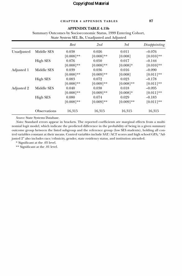
C H A P T E R 4 A P P E N D I X T A B L E S 87
APPENDIX TABLE 4.15bSummary Outcomes by Socioeconomic Status, 1999 Entering Cohort,
State System SEL Bs, Unadjusted and Adjusted
Best 2nd 3rd Disappointing
Unadjusted Middle SES 0.038 0.026 0.011 –0.076[0.008]** [0.008]** [0.008] [0.010]**
High SES 0.076 0.050 0.017 –0.144[0.008]** [0.008]** [0.008]* [0.010]**
Adjusted 1 Middle SES 0.039 0.036 0.016 –0.090[0.008]** [0.009]** [0.008] [0.011]**
High SES 0.083 0.072 0.023 –0.178[0.008]** [0.009]** [0.008]** [0.011]**
Adjusted 2 Middle SES 0.040 0.038 0.018 –0.095[0.008]** [0.009]** [0.008]* [0.011]**
High SES 0.080 0.074 0.029 –0.183[0.008]** [0.009]** [0.009]** [0.011]**
Observations 16,315 16,315 16,315 16,315
Source: State Systems Database.Notes: Standard errors appear in brackets. The reported coefficients are marginal effects from a multi-
nomial logit model, which indicate the predicted difference in the probability of being in a given summaryoutcome group between the listed subgroup and the reference group (low SES students), holding all con-trol variables constant at their means. Control variables include SAT/ACT scores and high school GPA; “Ad-justed 2” also includes race/ethnicity, gender, state residency status, and institution attended.
* Significant at the .05 level.** Significant at the .01 level.
Copyrighted MaterialCopyrighted MaterialCopyrighted Material

APPENDIX TABLE 4.16aSummary Outcomes by Race/Ethnicity and Gender, 1999 Entering Cohort,
Flagships and State System SEL As, Unadjusted and Adjusted
Best 2nd 3rd Disappointing
Unadjusted Black Males –0.175 –0.087 0.085 0.177[0.007]** [0.010]** [0.011]** [0.012]**
Hispanic Males –0.115 –0.022 0.052 0.086[0.009]** [0.012] [0.012]** [0.012]**
Asian Males 0.002 0.015 0.013 –0.030[0.007] [0.008]* [0.007] [0.006]**
White Females 0.151 0.018 –0.108 –0.060[0.004]** [0.004]** [0.003]** [0.003]**
Black Females –0.090 0.042 0.013 0.035[0.007]** [0.009]** [0.008] [0.008]**
Hispanic Females –0.011 0.033 –0.010 –0.012[0.011] [0.012]** [0.010] [0.010]
Asian Females 0.100 0.055 –0.065 –0.089[0.008]** [0.008]** [0.006]** [0.005]**
Adjusted 1 Black Males –0.102 –0.033 0.053 0.082[0.010]** [0.012]** [0.011]** [0.011]**
Hispanic Males –0.097 –0.018 0.044 0.070[0.009]** [0.013] [0.012]** [0.012]**
Asian Males –0.051 –0.003 0.037 0.018[0.006]** [0.008] [0.008]** [0.008]*
White Females 0.166 0.020 –0.121 –0.065[0.004]** [0.004]** [0.003]** [0.003]**
Black Females 0.011 0.077 –0.046 –0.041[0.010] [0.011]** [0.008]** [0.007]**
Hispanic Females 0.041 0.041 –0.043 –0.040[0.012]** [0.012]** [0.010]** [0.009]**
Asian Females 0.053 0.059 –0.056 –0.056[0.007]** [0.008]** [0.007]** [0.006]**
Adjusted 2 Black Males –0.098 –0.065 0.065 0.098[0.010]** [0.013]** [0.012]** [0.011]**
Hispanic Males –0.083 –0.029 0.039 0.073[0.010]** [0.013]* [0.012]** [0.012]**
Asian Males –0.029 0.002 0.032 –0.005[0.007]** [0.009] [0.008]** [0.007]
White Females 0.160 0.015 –0.117 –0.058[0.004]** [0.004]** [0.003]** [0.003]**
Black Females 0.021 0.047 –0.034 –0.034[0.011]* [0.011]** [0.009]** [0.007]**
Hispanic Females 0.065 0.021 –0.052 –0.035[0.013]** [0.013] [0.010]** [0.009]**
Asian Females 0.081 0.051 –0.065 –0.067[0.008]** [0.009]** [0.007]** [0.006]**
Observations 76,573 76,573 76,573 76,573
Source: Flagships Database and State Systems Database.Notes: Standard errors appear in brackets. The reported coefficients are marginal effects from a multi-
nomial logit model, which indicate the predicted difference in the probability of being in a given summaryoutcome group between the listed subgroup and the reference group (white males), holding all control vari-ables constant at their means. Control variables include SAT/ACT scores and high school GPA; “Adjusted 2”also includes income quartile, state residency status, and institution attended.
* Significant at the .05 level.** Significant at the .01 level.
Copyrighted MaterialCopyrighted MaterialCopyrighted Material

C H A P T E R 4 A P P E N D I X T A B L E S 89
APPENDIX TABLE 4.16bSummary Outcomes by Race and Gender, 1999 Entering Cohort,
State System SEL Bs, Unadjusted and Adjusted
Best 2nd 3rd Disappointing
Unadjusted Black Males –0.073 –0.064 0.024 0.113[0.007]** [0.010]** [0.013] [0.015]**
White Females 0.126 0.035 –0.077 –0.085[0.005]** [0.005]** [0.005]** [0.006]**
Black Females 0.007 –0.013 –0.027 0.032[0.007] [0.008] [0.009]** [0.011]**
Adjusted 1 Black Males –0.031 –0.031 0.012 0.051[0.009]** [0.013]* [0.013] [0.016]**
White Females 0.099 0.043 –0.074 –0.068[0.004]** [0.005]** [0.005]** [0.007]**
Black Females 0.053 0.014 –0.044 –0.023[0.009]** [0.010] [0.009]** [0.012]
Adjusted 2 Black Males –0.029 –0.023 0.011 0.041[0.008]** [0.014] [0.014] [0.017]*
White Females 0.081 0.044 –0.075 –0.050[0.004]** [0.006]** [0.005]** [0.007]**
Black Females 0.059 0.031 –0.048 –0.043[0.009]** [0.011]** [0.010]** [0.013]**
Observations 33,874 33,874 33,874 33,874
Source: State Systems Database.Notes: Standard errors appear in brackets. The reported coefficients are marginal effects from a multi-
nomial logit model, which indicate the predicted difference in the probability of being in a given summaryoutcome group between the listed subgroup and the reference group (white males), holding all control vari-ables constant at their means. Control variables include high school GPA and SAT/ACT scores; “Adjusted 2”also includes income quartile, state residency status, and institution attended.
* Significant at the .05 level.** Significant at the .01 level.
Copyrighted MaterialCopyrighted MaterialCopyrighted Material

90 C H A P T E R 5 A P P E N D I X T A B L E S
APPENDIX TABLE 5.1Six-Year Graduation Rates by Mean SAT/ACT Score of High School,
National Data
Flagships and State System SEL As
Mean SAT/ACT Score 0.044 0.033 0.021 0.009[0.004]** [0.004]** [0.004]** [0.004]*
Controls for High School Size No Yes Yes Yesand Neighborhood Wealth?
Standard Controls Excluding No No Yes YesSAT/ACT?
Standard Controls Including No No No YesSAT/ACT?
Observations 61,640 61,640 61,640 61,640
State System SEL Bs
Mean SAT/ACT Score 0.042 0.039 0.027 0.011[0.006]** [0.007]** [0.006]** [0.006]
Controls for High School Size No Yes Yes Yesand Neighborhood Wealth?
Standard Controls Excluding No No Yes YesSAT/ACT?
Standard Controls Including No No No YesSAT/ACT?
Observations 28,527 28,527 28,527 28,527
Source: Flagships Database, State Systems Database, and National High School Database.Notes: Robust standard errors adjusted for clustering at the high school level appear in
brackets. Coefficients indicate the increase in six-year graduation rates associated with every100-point increase in the mean SAT/ACT score of the high school. Standard controls in-clude race/ethnicity, gender, university dummy variables, and family income.
* Significant at the .05 level.** Significant at the .01 level.
Copyrighted MaterialCopyrighted MaterialCopyrighted Material
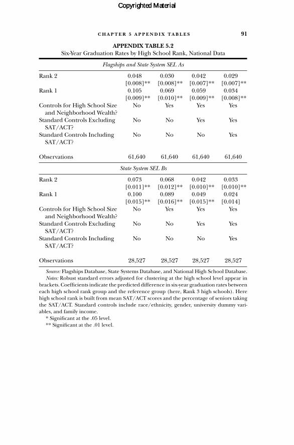
APPENDIX TABLE 5.2Six-Year Graduation Rates by High School Rank, National Data
Flagships and State System SEL As
Rank 2 0.048 0.030 0.042 0.029[0.008]** [0.008]** [0.007]** [0.007]**
Rank 1 0.105 0.069 0.059 0.034[0.009]** [0.010]** [0.009]** [0.008]**
Controls for High School Size No Yes Yes Yesand Neighborhood Wealth?
Standard Controls Excluding No No Yes YesSAT/ACT?
Standard Controls Including No No No YesSAT/ACT?
Observations 61,640 61,640 61,640 61,640
State System SEL Bs
Rank 2 0.073 0.068 0.042 0.033[0.011]** [0.012]** [0.010]** [0.010]**
Rank 1 0.100 0.089 0.049 0.024[0.015]** [0.016]** [0.015]** [0.014]
Controls for High School Size No Yes Yes Yesand Neighborhood Wealth?
Standard Controls Excluding No No Yes YesSAT/ACT?
Standard Controls Including No No No YesSAT/ACT?
Observations 28,527 28,527 28,527 28,527
Source: Flagships Database, State Systems Database, and National High School Database.Notes: Robust standard errors adjusted for clustering at the high school level appear in
brackets. Coefficients indicate the predicted difference in six-year graduation rates betweeneach high school rank group and the reference group (here, Rank 3 high schools). Herehigh school rank is built from mean SAT/ACT scores and the percentage of seniors takingthe SAT/ACT. Standard controls include race/ethnicity, gender, university dummy vari-ables, and family income.
* Significant at the .05 level.** Significant at the .01 level.
C H A P T E R 5 A P P E N D I X T A B L E S 91
Copyrighted MaterialCopyrighted MaterialCopyrighted Material
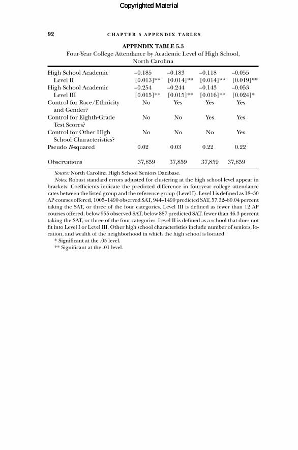
92 C H A P T E R 5 A P P E N D I X T A B L E S
APPENDIX TABLE 5.3Four-Year College Attendance by Academic Level of High School,
North Carolina
High School Academic –0.185 –0.183 –0.118 –0.055Level II [0.013]** [0.014]** [0.014]** [0.019]**
High School Academic –0.254 –0.244 –0.143 –0.053Level III [0.015]** [0.015]** [0.016]** [0.024]*
Control for Race/Ethnicity No Yes Yes Yes and Gender?
Control for Eighth-Grade No No Yes YesTest Scores?
Control for Other High No No No YesSchool Characteristics?
Pseudo R-squared 0.02 0.03 0.22 0.22
Observations 37,859 37,859 37,859 37,859
Source: North Carolina High School Seniors Database.Notes: Robust standard errors adjusted for clustering at the high school level appear in
brackets. Coefficients indicate the predicted difference in four-year college attendancerates between the listed group and the reference group (Level I). Level I is defined as 18–30AP courses offered, 1005–1490 observed SAT, 944–1490 predicted SAT, 57.32–80.04 percenttaking the SAT, or three of the four categories. Level III is defined as fewer than 12 APcourses offered, below 955 observed SAT, below 887 predicted SAT, fewer than 46.3 percenttaking the SAT, or three of the four categories. Level II is defined as a school that does notfit into Level I or Level III. Other high school characteristics include number of seniors, lo-cation, and wealth of the neighborhood in which the high school is located.
* Significant at the .05 level.** Significant at the .01 level.
Copyrighted MaterialCopyrighted MaterialCopyrighted Material
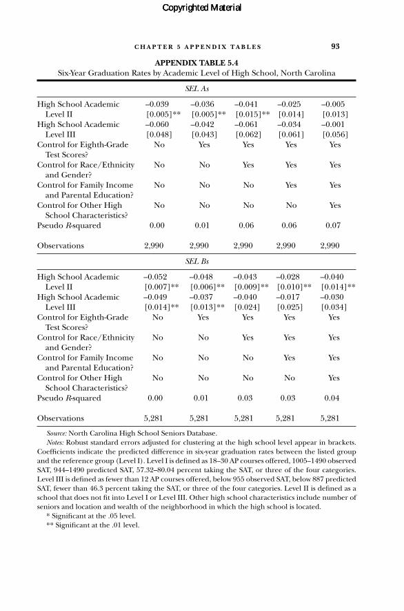
C H A P T E R 5 A P P E N D I X T A B L E S 93
APPENDIX TABLE 5.4Six-Year Graduation Rates by Academic Level of High School, North Carolina
SEL As
High School Academic –0.039 –0.036 –0.041 –0.025 –0.005Level II [0.005]** [0.005]** [0.015]** [0.014] [0.013]
High School Academic –0.060 –0.042 –0.061 –0.034 –0.001Level III [0.048] [0.043] [0.062] [0.061] [0.056]
Control for Eighth-Grade No Yes Yes Yes YesTest Scores?
Control for Race/Ethnicity No No Yes Yes Yesand Gender?
Control for Family Income No No No Yes Yesand Parental Education?
Control for Other High No No No No YesSchool Characteristics?
Pseudo R-squared 0.00 0.01 0.06 0.06 0.07
Observations 2,990 2,990 2,990 2,990 2,990
SEL Bs
High School Academic –0.052 –0.048 –0.043 –0.028 –0.040Level II [0.007]** [0.006]** [0.009]** [0.010]** [0.014]**
High School Academic –0.049 –0.037 –0.040 –0.017 –0.030Level III [0.014]** [0.013]** [0.024] [0.025] [0.034]
Control for Eighth-Grade No Yes Yes Yes YesTest Scores?
Control for Race/Ethnicity No No Yes Yes Yesand Gender?
Control for Family Income No No No Yes Yesand Parental Education?
Control for Other High No No No No YesSchool Characteristics?
Pseudo R-squared 0.00 0.01 0.03 0.03 0.04
Observations 5,281 5,281 5,281 5,281 5,281
Source: North Carolina High School Seniors Database.Notes: Robust standard errors adjusted for clustering at the high school level appear in brackets.
Coefficients indicate the predicted difference in six-year graduation rates between the listed groupand the reference group (Level I). Level I is defined as 18–30 AP courses offered, 1005–1490 observedSAT, 944–1490 predicted SAT, 57.32–80.04 percent taking the SAT, or three of the four categories.Level III is defined as fewer than 12 AP courses offered, below 955 observed SAT, below 887 predictedSAT, fewer than 46.3 percent taking the SAT, or three of the four categories. Level II is defined as aschool that does not fit into Level I or Level III. Other high school characteristics include number ofseniors and location and wealth of the neighborhood in which the high school is located.
* Significant at the .05 level.** Significant at the .01 level.
Copyrighted MaterialCopyrighted MaterialCopyrighted Material

94 C H A P T E R 5 A P P E N D I X T A B L E S
APPENDIX TABLE 5.5Six-Year Graduation Rates by Academic Level of High School and within
University-Reported High School GPA Ranges, North Carolina
SEL As
All Students 2.5–2.99 3.0–3.49 3.5–4.0 Above 4.0
High School Academic –0.039 –0.006 — 0.076 –0.009 –0.014Level II [0.005]** [0.013] — [0.053] [0.051] [0.008]
High School Academic –0.062 –0.003 — 0.152 0.053 –0.077Level III [0.046] [0.055] — [0.075]* [0.077] [0.016]**
Standard Controls? No Yes — Yes Yes YesPseudo R-Squared 0.00 0.07 — 0.14 0.07 0.05
Observations 2,996 2,996 — 200 1,092 1,655
SEL Bs
All Students Below 2.5 2.5–2.99 3.0–3.49 3.5–4.0
High School Academic –0.052 –0.042 –0.050 –0.028 –0.093 –0.045Level II [0.007]** [0.014]** [0.138] [0.036] [0.030]** [0.030]
High School Academic –0.050 –0.033 –0.065 –0.088 –0.103 –0.037Level III [0.014]** [0.034] [0.133] [0.085] [0.074] [0.033]
Standard Controls? No Yes Yes Yes Yes YesPseudo R-Squared 0.00 0.04 0.18 0.04 0.05 0.04
Observations 5,310 5,310 147 792 1,799 2,556
Source: North Carolina High School Seniors Database.Notes: Robust standard errors adjusted for clustering at the high school level appear in brackets. Coeffi-
cients indicate the predicted difference in six-year graduation rates between the listed group and the refer-ence group (Level I). Level I is defined as 18–30 AP courses offered, 1005–1490 observed SAT, 944–1490 pre-dicted SAT, 57.32–80.04 percent taking the SAT, or three of the four categories. Level III is defined as fewerthan 12 AP courses offered, below 955 observed SAT, below 887 predicted SAT, fewer than 46.3 percent tak-ing the SAT, or three of the four categories. Level II is defined as a school that does not fit into Level I orLevel III. Standard controls include race/ethnicity, gender, eighth-grade test scores, family income, parentaleducation, indicators for university attended, the number of seniors in the high school, the wealth of theneighborhood of the high school, and the location of the high school.
* Significant at the .05 level.** Significant at the .01 level.
Copyrighted MaterialCopyrighted MaterialCopyrighted Material

C H A P T E R 5 A P P E N D I X T A B L E S 95
APPENDIX TABLE 5.6Undermatch Rates by Parental Education and Family Income, North Carolina
Parental Education
Some College –0.114 –0.119 –0.109 –0.107 –0.084[0.022]** [0.022]** [0.023]** [0.023]** [0.024]**
College Degree –0.203 –0.205 –0.175 –0.159 –0.106[0.022]** [0.022]** [0.021]** [0.022]** [0.023]**
Graduate Degree –0.300 –0.296 –0.258 –0.225 –0.142[0.021]** [0.021]** [0.022]** [0.023]** [0.024]**
Control for Race/Ethnicity No Yes Yes Yes Yes and Gender?
Control for High School No No Yes Yes YesCharacteristics and Academic Level?
Control for SAT Scores and No No No Yes YesHigh School GPA?
Control for Family Income? No No No No YesPseudo R-squared 0.03 0.04 0.05 0.08 0.09
Observations 5,211 5,211 5,211 5,211 5,211
Family Income
Second Quartile –0.037 –0.042 –0.039 –0.041 –0.029[0.025] [0.025] [0.026] [0.026] [0.026]
Third Quartile –0.169 –0.177 –0.163 –0.154 –0.123[0.023]** [0.024]** [0.024]** [0.025]** [0.025]**
Top Quartile –0.308 –0.313 –0.283 –0.267 –0.224[0.023]** [0.023]** [0.024]** [0.024]** [0.025]**
Control for Race/Ethnicity and Gender? No Yes Yes Yes Yes
Control for High School Characteristics and Academic Level? No No Yes Yes Yes
Control for SAT Scores and High School GPA? No No No Yes Yes
Control for Parental Education? No No No No Yes
Pseudo R-squared 0.04 0.05 0.06 0.09 0.09
Observations 5,211 5,211 5,211 5,211 5,211
Source: North Carolina High School Seniors Database.Notes: Robust standard errors adjusted for clustering at the high school level appear in brackets. Coeffi-
cients indicate the predicted difference in the undermatch rate between the listed group and the referencegroup (no college in the case of parental education and bottom quartile in the case of family income). Highschool characteristics include number of seniors, location, and the wealth of the neighborhood in which thehigh school is located.
* Significant at the .05 level.** Significant at the .01 level.
Copyrighted MaterialCopyrighted MaterialCopyrighted Material
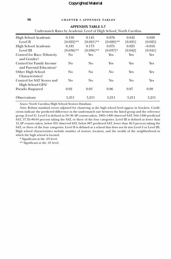
96 C H A P T E R 5 A P P E N D I X T A B L E S
APPENDIX TABLE 5.7Undermatch Rates by Academic Level of High School, North Carolina
High School Academic 0.150 0.145 0.076 0.042 0.020Level II [0.022]** [0.021]** [0.020]** [0.025] [0.025]
High School Academic 0.185 0.173 0.075 0.025 –0.016Level III [0.036]** [0.036]** [0.037]* [0.042] [0.041]
Control for Race/Ethnicity No Yes Yes Yes Yes and Gender?
Control for Family Income No No Yes Yes Yesand Parental Education?
Other High School No No No Yes YesCharacteristics?
Control for SAT Scores and No No No No YesHigh School GPA?
Pseudo R-squared 0.02 0.03 0.06 0.07 0.09
Observations 5,211 5,211 5,211 5,211 5,211
Source: North Carolina High School Seniors Database.Notes: Robust standard errors adjusted for clustering at the high school level appear in brackets. Coeffi-
cients indicate the predicted difference in the undermatch rate between the listed group and the referencegroup (Level I). Level I is defined as 18–30 AP courses taken, 1005–1490 observed SAT, 944–1490 predictedSAT, 57.32–80.04 percent taking the SAT, or three of the four categories. Level III is defined as fewer than12 AP courses taken, below 955 observed SAT, below 887 predicted SAT, fewer than 46.3 percent taking theSAT, or three of the four categories. Level II is defined as a school that does not fit into Level I or Level III.High school characteristics include number of seniors, location, and the wealth of the neighborhood inwhich the high school is located.
* Significant at the .05 level.** Significant at the .01 level.
Copyrighted MaterialCopyrighted MaterialCopyrighted Material

C H A P T E R 5 A P P E N D I X T A B L E S 97
APPENDIX TABLE 5.8Graduation Rates by Undermatch Status, North Carolina
Six-Year Graduation Rates
Undermatched from a SEL A –0.143 –0.107 –0.091 –0.084to a SEL B (0/1) [0.017]** [0.017]** [0.017]** [0.019]**
Include Standard Controls? No Yes Yes YesControl for Family Income and No No Yes Yes
Parental Education?High School Fixed Effects? No No No YesPseudo R-squared 0.02 0.06 0.07 0.13
Observations 3,608 3,608 3,608 3,439
Four-Year Graduation Rates
Undermatched from a SEL A –0.149 –0.117 –0.097 –0.099to a SEL B (0/1) [0.018]** [0.020]** [0.020]** [0.022]**
Include Standard Controls? No Yes Yes YesControl for Family Income and No No Yes Yes
Parental Education?High School Fixed Effects? No No No YesPseudo R-squared 0.01 0.07 0.08 0.14
Observations 3,608 3,608 3,608 3,521
Source: North Carolina High School Seniors Database.Notes: Standard errors adjusted for clustering at the university level appear in brackets. Standard controls
include SAT scores, adjusted high school GPA, race/ethnicity, and gender. These regressions are run onlyon students who attended a SEL A or a SEL B and had the academic qualifications to be presumed eligiblefor a SEL A.
* Significant at the .05 level.** Significant at the .01 level.
Copyrighted MaterialCopyrighted MaterialCopyrighted Material

98 C H A P T E R 5 A P P E N D I X T A B L E S
APPENDIX TABLE 5.9College-Going Patterns of Students in the Top Quartile of the
Eighth-Grade Test Score Distribution by Academic Level of High School, North Carolina (Percent)
Enrolled at a No CollegeTwo-Year College Enrollment Sub-Totals
Level I High School 5 15 20Level II High School 13 18 31Level III High School 15 23 38All Levels 11 18 29
Source: North Carolina High School Seniors Database.Notes: Level I is defined as 18–30 AP courses offered, 1005–1490 observed SAT, 944–1490 predicted SAT,
57.32–80.04 percent taking the SAT, or three of the four categories. Level III is defined as fewer than 12 APcourses offered, below 955 observed SAT, below 887 predicted SAT, fewer than 46.3 percent taking the SAT,or three of the four categories. Level II is defined as a school that does not fit into Level I or Level III.
Copyrighted MaterialCopyrighted MaterialCopyrighted Material
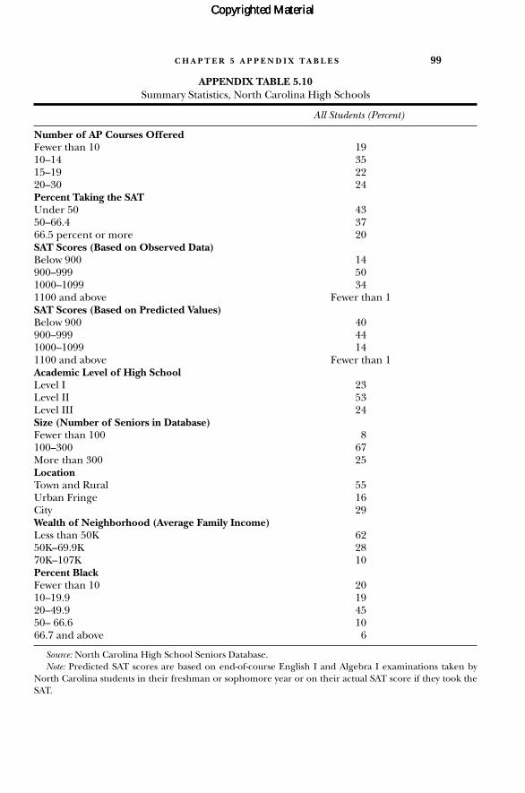
C H A P T E R 5 A P P E N D I X T A B L E S 99
APPENDIX TABLE 5.10Summary Statistics, North Carolina High Schools
All Students (Percent)
Number of AP Courses OfferedFewer than 10 1910–14 3515–19 2220–30 24Percent Taking the SATUnder 50 4350–66.4 3766.5 percent or more 20SAT Scores (Based on Observed Data)Below 900 14900–999 501000–1099 341100 and above Fewer than 1SAT Scores (Based on Predicted Values)Below 900 40900–999 441000–1099 141100 and above Fewer than 1Academic Level of High SchoolLevel I 23Level II 53Level III 24Size (Number of Seniors in Database)Fewer than 100 8100–300 67More than 300 25LocationTown and Rural 55Urban Fringe 16City 29Wealth of Neighborhood (Average Family Income)Less than 50K 6250K–69.9K 2870K–107K 10Percent BlackFewer than 10 2010–19.9 1920–49.9 4550– 66.6 1066.7 and above 6
Source: North Carolina High School Seniors Database.Note: Predicted SAT scores are based on end-of-course English I and Algebra I examinations taken by
North Carolina students in their freshman or sophomore year or on their actual SAT score if they took theSAT.
Copyrighted MaterialCopyrighted MaterialCopyrighted Material
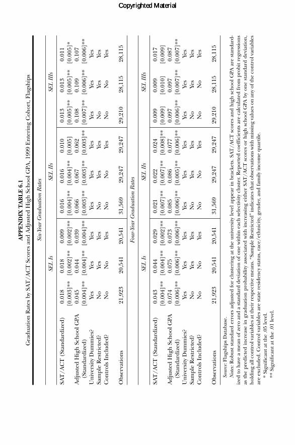
AP
PE
ND
IX T
AB
LE
6.1
Gra
duat
ion
Rat
es b
y SA
T/A
CT
Sco
res
and
Adj
uste
d H
igh
Sch
ool G
PA, 1
999
En
teri
ng
Coh
ort,
Flag
ship
s
Six-
Year
Gra
duat
ion
Rat
es
SEL
Is
SEL
IIs
SEL
III
s
SAT
/AC
T (
Stan
dard
ized
)0.
018
0.01
80.
009
0.01
60.
016
0.01
00.
013
0.01
30.
011
[0.0
03]*
*[0
.002
]**
[0.0
02]*
*[0
.004
]**
[0.0
04]*
*[0
.005
][0
.005
]**
[0.0
05]*
*[0
.005
]*A
djus
ted
Hig
h S
choo
l GPA
0.
045
0.04
40.
039
0.06
60.
067
0.06
20.
108
0.10
90.
107
(Sta
nda
rdiz
ed)
[0.0
04]*
*[0
.004
]**
[0.0
04]*
*[0
.003
]**
[0.0
03]*
*[0
.003
]**
[0.0
07]*
*[0
.006
]**
[0.0
06]*
*U
niv
ersi
ty D
umm
ies?
Yes
Yes
Yes
Yes
Yes
Yes
Yes
Yes
Yes
Sam
ple
Res
tric
ted?
No
Yes
Yes
No
Yes
Yes
No
Yes
Yes
Con
trol
s In
clud
ed?
No
No
Yes
No
No
Yes
No
No
Yes
Obs
erva
tion
s21
,923
20,5
4120
,541
31,5
6929
,247
29,2
4729
,210
28,1
1528
,115
Four
-Yea
r G
radu
atio
n R
ates
SEL
Is
SEL
IIs
SEL
III
s
SAT
/AC
T (
Stan
dard
ized
)0.
043
0.04
40.
029
0.02
10.
022
0.02
40.
009
0.00
90.
017
[0.0
04]*
*[0
.004
]**
[0.0
02]*
*[0
.007
]**
[0.0
07]*
*[0
.008
]**
[0.0
09]
[0.0
10]
[0.0
09]
Adj
uste
d H
igh
Sch
ool G
PA
0.07
40.
075
0.07
30.
085
0.08
60.
077
0.09
70.
097
0.08
7(S
tan
dard
ized
)[0
.006
]**
[0.0
06]*
*[0
.006
]**
[0.0
06]*
*[0
.005
]**
[0.0
06]*
*[0
.006
]**
[0.0
07]*
*[0
.007
]**
Un
iver
sity
Dum
mie
s?Ye
sYe
sYe
sYe
sYe
sYe
sYe
sYe
sYe
sSa
mpl
e R
estr
icte
d?N
oYe
sYe
sN
oYe
sYe
sN
oYe
sYe
sC
ontr
ols
Incl
uded
?N
oN
oYe
sN
oN
oYe
sN
oN
oYe
s
Obs
erva
tion
s21
,923
20,5
4120
,541
31,5
6929
,247
29,2
4729
,210
28,1
1528
,115
Sour
ce:F
lags
hip
s D
atab
ase.
Not
es:R
obus
t st
anda
rd e
rror
s ad
just
ed f
or c
lust
erin
g at
th
e un
iver
sity
leve
l app
ear
in b
rack
ets.
SA
T/A
CT
sco
res
and
hig
h s
choo
l GPA
are
sta
nda
rd-
ized
to h
ave
a m
ean
of z
ero
and
a st
anda
rd d
evia
tion
of o
ne
wit
hin
eac
h s
elec
tivi
ty c
lust
er. R
epor
ted
coef
fici
ents
are
cal
cula
ted
from
pro
bit r
egre
ssio
ns
as t
he
pred
icte
d in
crea
se in
gra
duat
ion
pro
babi
lity
asso
ciat
ed w
ith
incr
easi
ng
eith
er S
AT
/AC
T s
core
s or
hig
h s
choo
l GPA
by
one
stan
dard
dev
iati
on,
hol
din
g al
l con
trol
var
iabl
es a
t th
eir
resp
ecti
ve m
ean
s. “
Sam
ple
Res
tric
ted”
indi
cate
s th
at o
bser
vati
ons w
ith
mis
sin
g va
lues
on
an
y of
the
con
trol
var
iabl
esar
e ex
clud
ed. C
ontr
ol v
aria
bles
are
sta
te r
esid
ency
sta
tus,
rac
e/et
hn
icit
y, g
ende
r, an
d fa
mily
inco
me
quar
tile
.*
Sign
ifica
nt a
t th
e .0
5 le
vel.
** S
ign
ifica
nt a
t th
e .0
1 le
vel.
Copyrighted MaterialCopyrighted MaterialCopyrighted Material
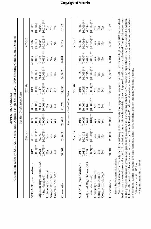
AP
PE
ND
IX T
AB
LE
6.2
Gra
duat
ion
Rat
es b
y SA
T/A
CT
Sco
res
and
Adj
uste
d H
igh
Sch
ool G
PA, 1
999
En
teri
ng
Coh
ort,
Stat
e Sy
stem
s
Six-
Year
Gra
duat
ion
Rat
es
SEL
As
SEL
Bs
HB
CU
s
SAT
/AC
T (
Stan
dard
ized
)0.
012
0.01
10.
007
0.01
20.
013
0.01
2–0
.007
–0.0
060.
007
[0.0
04]*
*[0
.004
]**
[0.0
04]
[0.0
08]
[0.0
08]
[0.0
07]
[0.0
06]
[0.0
07]
[0.0
06]
Adj
uste
d H
igh
Sch
ool G
PA
0.07
20.
073
0.06
80.
116
0.11
70.
115
0.10
80.
109
0.10
4(S
tan
dard
ized
)[0
.007
]**
[0.0
07]*
*[0
.006
]**
[0.0
08]*
*[0
.008
]**
[0.0
08]*
*[0
.012
]**
[0.0
12]*
*[0
.011
]**
Un
iver
sity
Dum
mie
s?Ye
sYe
sYe
sYe
sYe
sYe
sYe
sYe
sYe
sSa
mpl
e R
estr
icte
d?N
oYe
sYe
sN
oYe
sYe
sN
oYe
sYe
sC
ontr
ols
Incl
uded
?N
oN
oYe
sN
oN
oYe
sN
oN
oYe
s
Obs
erva
tion
s30
,301
28,0
8328
,083
41,5
7338
,382
38,3
826,
481
6,12
26,
122
Four
-Yea
r G
radu
atio
n R
ates
SEL
As
SEL
Bs
HB
CU
s
SAT
/AC
T (
Stan
dard
ized
)0.
011
0.01
10.
016
0.00
90.
010
0.01
80.
015
0.01
60.
026
[0.0
11]
[0.0
11]
[0.0
09]
[0.0
05]
[0.0
05]
[0.0
05]*
*[0
.006
]*[0
.006
]*[0
.006
]**
Adj
uste
d H
igh
Sch
ool G
PA
0.10
80.
108
0.09
40.
104
0.10
40.
095
0.09
30.
092
0.08
4(S
tan
dard
ized
)[0
.009
]**
[0.0
09]*
*[0
.010
]**
[0.0
04]*
*[0
.004
]**
[0.0
04]*
*[0
.005
]**
[0.0
05]*
*[0
.004
]**
Un
iver
sity
Dum
mie
s?Ye
sYe
sYe
sYe
sYe
sYe
sYe
sYe
sYe
sSa
mpl
e R
estr
icte
d?N
oYe
sYe
sN
oYe
sYe
sN
oYe
sYe
sC
ontr
ols
Incl
uded
?N
oN
oYe
sN
oN
oYe
sN
oN
oYe
s
Obs
erva
tion
s30
,301
28,0
8328
,083
41,5
7338
,382
38,3
826,
481
6,12
26,
122
Sour
ce:S
tate
Sys
tem
s D
atab
ase.
Not
es:R
obus
t st
anda
rd e
rror
s ad
just
ed f
or c
lust
erin
g at
th
e un
iver
sity
leve
l app
ear
in b
rack
ets.
SA
T/A
CT
sco
res
and
hig
h s
choo
l GPA
are
sta
nda
rd-
ized
to h
ave
a m
ean
of z
ero
and
a st
anda
rd d
evia
tion
of o
ne
wit
hin
eac
h s
elec
tivi
ty c
lust
er. R
epor
ted
coef
fici
ents
are
cal
cula
ted
from
pro
bit r
egre
ssio
ns
as t
he
pred
icte
d in
crea
se in
gra
duat
ion
pro
babi
lity
asso
ciat
ed w
ith
incr
easi
ng
eith
er S
AT
/AC
T s
core
s or
hig
h s
choo
l GPA
by
one
stan
dard
dev
iati
on,
hol
din
g al
l con
trol
var
iabl
es a
t th
eir
resp
ecti
ve m
ean
s. “
Sam
ple
Res
tric
ted”
indi
cate
s th
at o
bser
vati
ons w
ith
mis
sin
g va
lues
on
an
y of
the
con
trol
var
iabl
esar
e ex
clud
ed. C
ontr
ol v
aria
bles
are
sta
te r
esid
ency
sta
tus,
rac
e/et
hn
icit
y, g
ende
r, an
d fa
mily
inco
me
quar
tile
.*
Sign
ifica
nt a
t th
e .0
5 le
vel.
** S
ign
ifica
nt a
t th
e .0
1 le
vel.
Copyrighted MaterialCopyrighted MaterialCopyrighted Material

AP
PE
ND
IX T
AB
LE
6.3
Gra
duat
ion
Rat
es b
y SA
T S
core
s, A
CT
Sco
res,
an
d A
djus
ted
Hig
h S
choo
l GPA
, 199
9 E
nte
rin
g C
ohor
t
Flag
ship
s
Six-
Year
Gra
duat
ion
Rat
esFo
ur-Y
ear
Gra
duat
ion
Rat
es
Adj
uste
d H
igh
Sch
ool G
PA
0.07
00.
067
0.06
90.
067
0.09
40.
088
0.08
90.
086
(Sta
nda
rdiz
ed)
[0.0
05]*
*[0
.005
]**
[0.0
05]*
*[0
.006
]**
[0.0
06]*
*[0
.006
]**
[0.0
05]*
*[0
.005
]**
SAT
Sco
res
(Sta
nda
rdiz
ed)
0.01
10.
007
0.01
80.
020
[0.0
04]*
*[0
.004
][0
.009
][0
.009
]*A
CT
Sco
res
(Sta
nda
rdiz
ed)
0.01
40.
008
0.03
00.
025
[0.0
05]*
*[0
.005
][0
.008
]**
[0.0
08]*
*A
ddit
ion
al C
ontr
ols?
No
Yes
No
Yes
No
Yes
No
Yes
Obs
erva
tion
s25
,046
24,0
8325
,046
24,0
8325
,046
24,0
8325
,046
24,0
83
Ohi
o SE
L B
s
Six-
Year
Gra
duat
ion
Rat
esFo
ur-Y
ear
Gra
duat
ion
Rat
es
Adj
uste
d H
igh
Sch
ool G
PA
0.15
20.
148
0.15
40.
152
0.12
30.
106
0.11
80.
104
(Sta
nda
rdiz
ed)
[0.0
12]*
*[0
.010
]**
[0.0
13]*
*[0
.012
]**
[0.0
05]*
*[0
.006
]**
[0.0
07]*
*[0
.007
]**
SAT
Sco
res
(Sta
nda
rdiz
ed)
0.01
00.
006
–0.0
020.
013
[0.0
09]
[0.0
10]
[0.0
08]
[0.0
07]
AC
T S
core
s (S
tan
dard
ized
)0.
007
–0.0
010.
007
0.01
6[0
.008
][0
.007
][0
.007
][0
.006
]**
Add
itio
nal
Con
trol
s?N
oYe
sN
oYe
sN
oYe
sN
oYe
s
Obs
erva
tion
s7,
533
7,32
67,
533
7,32
67,
533
7,31
17,
533
7,31
1
Sour
ce:F
lags
hip
s D
atab
ase
and
Stat
e Sy
stem
s D
atab
ase.
Not
es:R
obus
t sta
nda
rd e
rror
s ad
just
ed fo
r cl
uste
rin
g at
the
univ
ersi
ty le
vel a
ppea
r in
bra
cket
s. S
AT
sco
res,
AC
T s
core
s, a
nd
hig
h s
choo
l GPA
are
sta
n-
dard
ized
to h
ave
a m
ean
of z
ero
and
a st
anda
rd d
evia
tion
of o
ne
sepa
rate
ly fo
r th
e fl
agsh
ips a
nd
Oh
io S
EL
Bs.
Rep
orte
d co
effi
cien
ts a
re c
alcu
late
d fr
ompr
obit
reg
ress
ion
s as
th
e pr
edic
ted
incr
ease
in g
radu
atio
n p
roba
bilit
y as
soci
ated
wit
h in
crea
sin
g ei
ther
SA
T s
core
s, A
CT
sco
res,
or
hig
h s
choo
l GPA
by
one
stan
dard
dev
iati
on, h
oldi
ng
all c
ontr
ol v
aria
bles
at
thei
r re
spec
tive
mea
ns.
All
regr
essi
ons
incl
ude
univ
ersi
ty in
dica
tors
an
d ar
e ba
sed
only
on
stu
-de
nts
wh
o to
ok b
oth
the
SAT
an
d th
e A
CT.
“A
ddit
ion
al C
ontr
ols”
incl
ude
race
/eth
nic
ity,
gen
der,
stat
e re
side
ncy
sta
tus,
an
d fa
mily
inco
me
quar
tile
.*
Sign
ifica
nt a
t th
e .0
5 le
vel.
** S
ign
ifica
nt a
t th
e .0
1 le
vel.
Copyrighted MaterialCopyrighted MaterialCopyrighted Material
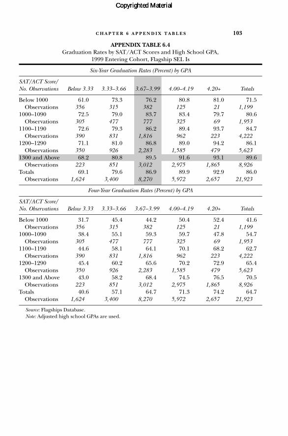
C H A P T E R 6 A P P E N D I X T A B L E S 103
APPENDIX TABLE 6.4Graduation Rates by SAT/ACT Scores and High School GPA,
1999 Entering Cohort, Flagship SEL Is
Six-Year Graduation Rates (Percent) by GPA
SAT/ACT Score/No. Observations Below 3.33 3.33–3.66 3.67–3.99 4.00–4.19 4.20+ Totals
Below 1000 61.0 73.3 76.2 80.8 81.0 71.5Observations 356 315 382 125 21 1,199
1000–1090 72.5 79.0 83.7 83.4 79.7 80.6Observations 305 477 777 325 69 1,953
1100–1190 72.6 79.3 86.2 89.4 93.7 84.7Observations 390 831 1,816 962 223 4,222
1200–1290 71.1 81.0 86.8 89.0 94.2 86.1Observations 350 926 2,283 1,585 479 5,623
1300 and Above 68.2 80.8 89.5 91.6 93.1 89.6Observations 223 851 3,012 2,975 1,865 8,926
Totals 69.1 79.6 86.9 89.9 92.9 86.0Observations 1,624 3,400 8,270 5,972 2,657 21,923
Four-Year Graduation Rates (Percent) by GPA
SAT/ACT Score/No. Observations Below 3.33 3.33–3.66 3.67–3.99 4.00–4.19 4.20+ Totals
Below 1000 31.7 45.4 44.2 50.4 52.4 41.6Observations 356 315 382 125 21 1,199
1000–1090 38.4 55.1 59.3 59.7 47.8 54.7Observations 305 477 777 325 69 1,953
1100–1190 44.6 58.1 64.1 70.1 68.2 62.7Observations 390 831 1,816 962 223 4,222
1200–1290 45.4 60.2 65.6 70.2 72.9 65.4Observations 350 926 2,283 1,585 479 5,623
1300 and Above 43.0 58.2 68.4 74.5 76.5 70.5Observations 223 851 3,012 2,975 1,865 8,926
Totals 40.6 57.1 64.7 71.3 74.2 64.7Observations 1,624 3,400 8,270 5,972 2,657 21,923
Source: Flagships Database.Note: Adjusted high school GPAs are used.
Copyrighted MaterialCopyrighted MaterialCopyrighted Material

APPENDIX TABLE 6.5Graduation Rates by SAT/ACT Scores and High School GPA,
1999 Entering Cohort, Flagship SEL IIs
6-Year Graduation Rates (Percent) by GPA
SAT/ACT Score/No. Observations Below 3.33 3.33–3.66 3.67–3.99 4.00–4.19 4.20+ Totals
Below 1000 58.0 70.0 73.6 83.3 67.6Observations 1,045 820 954 156 2,975
1000–1090 65.9 75.0 79.5 84.1 83.3 76.2Observations 865 1,274 2,052 428 48 4,667
1100–1190 67.6 78.3 82.4 86.6 87.5 80.2Observations 1,039 1,941 4,077 1,055 160 8,272
1200–1290 67.0 78.8 82.4 87.7 87.1 81.5Observations 697 1,544 3,841 1,478 317 7,877
1300 and Above 59.9 72.2 83.7 87.9 93.6 83.2Observations 421 1,049 3,196 2,128 980 7,774
Totals 63.9 75.8 81.7 87.1 91.2 79.5Observations 4,067 6,628 14,120 5,245 1,505 31,565
Four-Year Graduation Rates (Percent) by GPA
SAT/ACT Score/No. Observations Below 3.33 3.33–3.66 3.67–3.99 4.00–4.19 4.20+ Totals
Below 1000 26.4 40.6 46.0 50.0 37.8Observations 1,045 820 954 156 2,975
1000–1090 37.0 48.2 51.4 58.6 60.4 48.6Observations 865 1,274 2,052 428 48 4,667
1100–1190 39.7 47.8 54.4 62.6 66.9 52.3Observations 1,039 1,941 4,077 1,055 160 8,272
1200–1290 37.4 49.2 53.9 61.4 66.9 53.4Observations 697 1,544 3,841 1,478 317 7,877
1300 and Above 34.4 44.5 54.8 63.2 71.9 56.8Observations 421 1,049 3,196 2,128 980 7,774
Totals 34.8 46.8 53.3 61.8 70.0 51.8Observations 4,067 6,628 14,120 5,245 1,505 31,565
Source: Flagships Database.Notes: Adjusted high school GPAs are used. Blank cells indicate that there were data on fewer than 15
students.
104 C H A P T E R 6 A P P E N D I X T A B L E S
Copyrighted MaterialCopyrighted MaterialCopyrighted Material

APPENDIX TABLE 6.6Graduation Rates by SAT/ACT Scores and High School GPA,
1999 Entering Cohort, Flagship SEL IIIs
Six-Year Graduation Rates (Percent) by GPA
SAT/ACT Score/No. Observations Below 3.00 3.00–3.32 3.33–3.66 3.67–3.99 4.00+ Totals
Below 900 46.1 54.8 57.1 70.7 53.7Observations 794 935 387 215 2,331
900–990 47.7 58.1 65.0 70.3 79.5 60.1Observations 994 1,893 1,080 988 39 4,994
1000–1090 49.1 60.0 66.0 72.0 82.9 63.7Observations 913 1,872 1,503 1,773 105 6,166
1100–1190 46.4 58.6 64.9 75.3 79.9 66.9Observations 668 1,708 1,636 3,172 314 7,498
1200 and Above 43.7 52.4 64.6 78.6 86.7 73.6Observations 311 911 1,354 4,107 1,531 8,214
Totals 47.1 57.6 64.6 75.5 85.3 65.9Observations 3,680 7,319 5,960 10,255 1,989 29,203
Four-Year Graduation Rates (Percent) by GPA
SAT/ACT Score/No. Observations Below 3.00 3.00–3.32 3.33–3.66 3.67–3.99 4.00+ Totals
Below 900 15.9 21.8 28.7 32.6 21.9Observations 794 935 387 215 2,331
900–990 17.6 26.8 33.1 36.4 33.3 28.3Observations 994 1,893 1,080 988 39 4,994
1000–1090 20.0 27.1 33.5 38.1 47.6 31.1Observations 913 1,872 1,503 1,773 105 6,166
1100–1190 18.6 25.9 32.5 39.6 47.5 33.4Observations 668 1,708 1,636 3,172 314 7,498
1200 and Above 13.8 20.2 31.3 42.9 53.3 39.3Observations 311 911 1,354 4,107 1,531 8,214
Totals 17.7 25.2 32.3 40.2 51.7 32.8Observations 3,680 7,319 5,960 10,255 1,989 29,203
Source: Flagships Database.Notes: Adjusted high school GPAs are used. Blank cells indicate that there were data on fewer than 15 students.
C H A P T E R 6 A P P E N D I X T A B L E S 105
Copyrighted MaterialCopyrighted MaterialCopyrighted Material
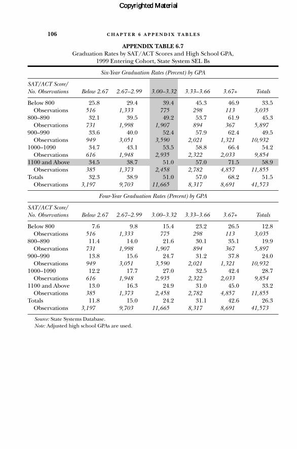
APPENDIX TABLE 6.7Graduation Rates by SAT/ACT Scores and High School GPA,
1999 Entering Cohort, State System SEL Bs
Six-Year Graduation Rates (Percent) by GPA
SAT/ACT Score/No. Observations Below 2.67 2.67–2.99 3.00–3.32 3.33–3.66 3.67+ Totals
Below 800 25.8 29.4 39.4 45.3 46.9 33.5Observations 516 1,333 775 298 113 3,035
800–890 32.1 39.5 49.2 53.7 61.9 45.3Observations 731 1,998 1,907 894 367 5,897
900–990 33.6 40.0 52.4 57.9 62.4 49.5Observations 949 3,051 3,590 2,021 1,321 10,932
1000–1090 34.7 43.1 53.5 58.8 66.4 54.2Observations 616 1,948 2,935 2,322 2,033 9,854
1100 and Above 34.5 38.7 51.0 57.0 71.5 58.9Observations 385 1,373 2,458 2,782 4,857 11,855
Totals 32.3 38.9 51.0 57.0 68.2 51.5Observations 3,197 9,703 11,665 8,317 8,691 41,573
Four-Year Graduation Rates (Percent) by GPA
SAT/ACT Score/No. Observations Below 2.67 2.67–2.99 3.00–3.32 3.33–3.66 3.67+ Totals
Below 800 7.6 9.8 15.4 23.2 26.5 12.8Observations 516 1,333 775 298 113 3,035
800–890 11.4 14.0 21.6 30.1 35.1 19.9Observations 731 1,998 1,907 894 367 5,897
900–990 13.8 15.6 24.7 31.2 37.8 24.0Observations 949 3,051 3,590 2,021 1,321 10,932
1000–1090 12.2 17.7 27.0 32.5 42.4 28.7Observations 616 1,948 2,935 2,322 2,033 9,854
1100 and Above 13.0 16.3 24.9 31.0 45.0 33.2Observations 385 1,373 2,458 2,782 4,857 11,855
Totals 11.8 15.0 24.2 31.1 42.6 26.3Observations 3,197 9,703 11,665 8,317 8,691 41,573
Source: State Systems Database.Note: Adjusted high school GPAs are used.
106 C H A P T E R 6 A P P E N D I X T A B L E S
Copyrighted MaterialCopyrighted MaterialCopyrighted Material
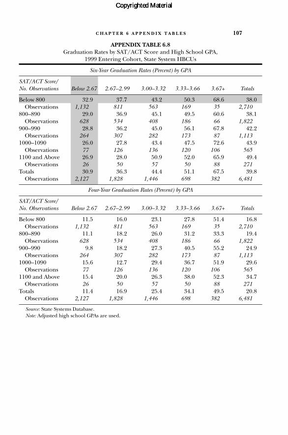
C H A P T E R 6 A P P E N D I X T A B L E S 107
APPENDIX TABLE 6.8Graduation Rates by SAT/ACT Score and High School GPA,
1999 Entering Cohort, State System HBCUs
Six-Year Graduation Rates (Percent) by GPA
SAT/ACT Score/No. Observations Below 2.67 2.67–2.99 3.00–3.32 3.33–3.66 3.67+ Totals
Below 800 32.9 37.7 43.2 50.3 68.6 38.0Observations 1,132 811 563 169 35 2,710
800–890 29.0 36.9 45.1 49.5 60.6 38.1Observations 628 534 408 186 66 1,822
900–990 28.8 36.2 45.0 56.1 67.8 42.2Observations 264 307 282 173 87 1,113
1000–1090 26.0 27.8 43.4 47.5 72.6 43.9Observations 77 126 136 120 106 565
1100 and Above 26.9 28.0 50.9 52.0 65.9 49.4Observations 26 50 57 50 88 271
Totals 30.9 36.3 44.4 51.1 67.5 39.8Observations 2,127 1,828 1,446 698 382 6,481
Four-Year Graduation Rates (Percent) by GPA
SAT/ACT Score/No. Observations Below 2.67 2.67–2.99 3.00–3.32 3.33–3.66 3.67+ Totals
Below 800 11.5 16.0 23.1 27.8 51.4 16.8Observations 1,132 811 563 169 35 2,710
800–890 11.1 18.2 26.0 31.2 33.3 19.4Observations 628 534 408 186 66 1,822
900–990 9.8 18.2 27.3 40.5 55.2 24.9Observations 264 307 282 173 87 1,113
1000–1090 15.6 12.7 29.4 36.7 51.9 29.6Observations 77 126 136 120 106 565
1100 and Above 15.4 20.0 26.3 38.0 52.3 34.7Observations 26 50 57 50 88 271
Totals 11.4 16.9 25.4 34.1 49.5 20.8Observations 2,127 1,828 1,446 698 382 6,481
Source: State Systems Database.Note: Adjusted high school GPAs are used.
Copyrighted MaterialCopyrighted MaterialCopyrighted Material

AP
PE
ND
IX T
AB
LE
6.9
aG
radu
atio
n R
ates
by
SAT
/AC
T S
core
an
d A
djus
ted
Hig
h S
choo
l GPA
, 199
9 E
nte
rin
g C
ohor
t, Fl
agsh
ips
Six-
Year
Gra
duat
ion
Rat
es
SEL
Is
SEL
IIs
SEL
III
s
SAT
/AC
T (
Stan
dard
ized
)0.
009
0.01
4–0
.014
0.01
00.
009
–0.0
130.
011
0.00
9–0
.007
[0.0
02]*
*[0
.003
]**
[0.0
05]*
*[0
.005
][0
.006
][0
.007
][0
.006
][0
.006
][0
.008
]A
djus
ted
Hig
h S
choo
l GPA
0.
040
0.04
70.
074
0.06
20.
068
0.09
60.
107
0.11
10.
142
(Sta
nda
rdiz
ed)
[0.0
04]*
*[0
.005
]**
[0.0
05]*
*[0
.003
]**
[0.0
04]*
*[0
.007
]**
[0.0
06]*
*[0
.007
]**
[0.0
07]*
*C
ontr
ols
Incl
uded
?Ye
sYe
sYe
sYe
sYe
sYe
sYe
sYe
sYe
sSa
mpl
e R
estr
icte
d?N
oYe
sYe
sN
oYe
sYe
sN
oYe
sYe
sH
igh
Sch
ool D
umm
ies?
No
No
Yes
No
No
Yes
No
No
Yes
Obs
erva
tion
s20
,531
13,6
7313
,673
29,1
8423
,635
23,6
3528
,097
24,2
8124
,281
Four
-Yea
r G
radu
atio
n R
ates
SEL
Is
SEL
IIs
SEL
III
s
SAT
/AC
T (
Stan
dard
ized
)0.
029
0.02
80.
001
0.02
40.
016
–0.0
010.
017
0.01
40.
009
[0.0
02]*
*[0
.005
]**
[0.0
07]
[0.0
08]*
*[0
.009
][0
.012
][0
.009
][0
.010
][0
.012
]A
djus
ted
Hig
h S
choo
l GPA
0.
073
0.07
80.
116
0.07
70.
084
0.11
20.
087
0.09
60.
118
(Sta
nda
rdiz
ed)
[0.0
06]*
*[0
.006
]**
[0.0
05]*
*[0
.006
]**
[0.0
07]*
*[0
.009
]**
[0.0
07]*
*[0
.007
]**
[0.0
07]*
*C
ontr
ols
Incl
uded
?Ye
sYe
sYe
sYe
sYe
sYe
sYe
sYe
sYe
sSa
mpl
e R
estr
icte
d?N
oYe
sYe
sN
oYe
sYe
sN
oYe
sYe
sH
igh
Sch
ool D
umm
ies?
No
No
Yes
No
No
Yes
No
No
Yes
Obs
erva
tion
s20
,531
16,7
9316
,793
29,1
8425
,672
25,6
7228
,097
24,1
2224
,122
Sour
ce:F
lags
hip
s D
atab
ase.
Not
es:R
obus
t st
anda
rd e
rror
s ad
just
ed f
or c
lust
erin
g at
th
e un
iver
sity
leve
l app
ear
in b
rack
ets.
SA
T/A
CT
sco
res
and
hig
h s
choo
l GPA
are
sta
nda
rd-
ized
to
hav
e a
mea
n o
f ze
ro a
nd
a st
anda
rd d
evia
tion
of
one
wit
hin
eac
h s
elec
tivi
ty c
lust
er (
befo
re t
he
sam
ple
is r
estr
icte
d). R
epor
ted
coef
fici
ents
are
calc
ulat
ed fr
om p
robi
t reg
ress
ion
s as
the
pred
icte
d in
crea
se in
gra
duat
ion
pro
babi
lity
asso
ciat
ed w
ith
incr
easi
ng
eith
er S
AT
/AC
T s
core
s or
hig
h s
choo
lG
PA b
y on
e st
anda
rd d
evia
tion
, hol
din
g al
l con
trol
var
iabl
es a
t th
eir
resp
ecti
ve m
ean
s. C
ontr
ol v
aria
bles
are
un
iver
sity
dum
mie
s, s
tate
res
iden
cy s
tatu
s,ra
ce/e
thn
icit
y, g
ende
r, an
d fa
mily
inco
me
quar
tile
. In
all
thre
e co
lum
ns,
the
sam
ple
is r
estr
icte
d to
stu
den
ts w
ith
non
-mis
sin
g va
lues
on
all
con
trol
var
i-ab
les.
“Sa
mpl
e R
estr
icte
d” in
dica
tes
that
th
e sa
mpl
e is
res
tric
ted
to s
tude
nts
th
at c
ame
from
hig
h s
choo
ls (
1) t
hat
sen
t at
leas
t tw
o st
uden
ts t
o th
e un
i-ve
rsit
ies
and
(2)
wh
ose
stud
ents
did
not
all
eith
er g
radu
ate
or fa
il to
gra
duat
e.*
Sign
ifica
nt a
t th
e .0
5 le
vel.
** S
ign
ifica
nt a
t th
e .0
1 le
vel.
Copyrighted MaterialCopyrighted MaterialCopyrighted Material

AP
PE
ND
IX T
AB
LE
6.9
bG
radu
atio
n R
ates
by
SAT
/AC
T S
core
s an
d A
djus
ted
Hig
h S
choo
l GPA
, 199
9 E
nte
rin
g C
ohor
t, St
ate
Syst
ems
Six-
Year
Gra
duat
ion
Rat
es
SEL
As
SEL
Bs
HB
CU
s
SAT
/AC
T (
Stan
dard
ized
)0.
007
0.00
6–0
.013
0.01
20.
011
–0.0
070.
007
0.00
4–0
.013
[0.0
04]
[0.0
04]
[0.0
05]*
*[0
.007
][0
.007
][0
.007
][0
.006
][0
.007
][0
.011
]A
djus
ted
Hig
h S
choo
l GPA
0.
068
0.07
40.
097
0.11
50.
119
0.14
70.
103
0.10
00.
130
(Sta
nda
rdiz
ed)
[0.0
06]*
*[0
.007
]**
[0.0
06]*
*[0
.008
]**
[0.0
08]*
*[0
.009
]**
[0.0
11]*
*[0
.010
]**
[0.0
11]*
*C
ontr
ols
Incl
uded
?Ye
sYe
sYe
sYe
sYe
sYe
sYe
sYe
sYe
sSa
mpl
e R
estr
icte
d?N
oYe
sYe
sN
oYe
sYe
sN
oYe
sYe
sH
igh
Sch
ool D
umm
ies?
No
No
Yes
No
No
Yes
No
No
Yes
Obs
erva
tion
s28
,067
24,3
4424
,344
38,3
5236
,559
36,5
596,
114
5,17
25,
172
Four
-Yea
r G
radu
atio
n R
ates
SEL
As
SEL
Bs
HB
CU
s
SAT
/AC
T (
Stan
dard
ized
)0.
016
0.01
3–0
.009
0.01
80.
015
0.00
50.
027
0.02
90.
014
[0.0
09]
[0.0
09]
[0.0
09]
[0.0
05]*
*[0
.005
]**
[0.0
05]
[0.0
06]*
*[0
.008
]**
[0.0
09]
Adj
uste
d H
igh
Sch
ool G
PA
0.09
40.
099
0.13
20.
095
0.10
20.
119
0.08
40.
095
0.11
0(S
tan
dard
ized
)[0
.010
]**
[0.0
10]*
*[0
.010
]**
[0.0
04]*
*[0
.004
]**
[0.0
04]*
*[0
.004
]**
[0.0
07]*
*[0
.009
]**
Con
trol
s In
clud
ed?
Yes
Yes
Yes
Yes
Yes
Yes
Yes
Yes
Yes
Sam
ple
Res
tric
ted?
No
Yes
Yes
No
Yes
Yes
No
Yes
Yes
Hig
h S
choo
l Dum
mie
s?N
oN
oYe
sN
oN
oYe
sN
oN
oYe
s
Obs
erva
tion
s28
,067
25,3
3525
,335
38,3
5235
,668
35,6
686,
114
4,64
64,
646
Sour
ce:S
tate
Sys
tem
s D
atab
ase.
Not
es:R
obus
t st
anda
rd e
rror
s ad
just
ed f
or c
lust
erin
g at
th
e un
iver
sity
leve
l app
ear
in b
rack
ets.
SA
T/A
CT
sco
res
and
hig
h s
choo
l GPA
are
sta
nda
rd-
ized
to
hav
e a
mea
n o
f ze
ro a
nd
a st
anda
rd d
evia
tion
of
one
wit
hin
eac
h s
elec
tivi
ty c
lust
er (
befo
re t
he
sam
ple
is r
estr
icte
d). R
epor
ted
coef
fici
ents
are
calc
ulat
ed fr
om p
robi
t reg
ress
ion
s as
the
pred
icte
d in
crea
se in
gra
duat
ion
pro
babi
lity
asso
ciat
ed w
ith
incr
easi
ng
eith
er S
AT
/AC
T s
core
s or
hig
h s
choo
lG
PA b
y on
e st
anda
rd d
evia
tion
, hol
din
g al
l con
trol
var
iabl
es a
t th
eir
resp
ecti
ve m
ean
s. C
ontr
ol v
aria
bles
are
un
iver
sity
dum
mie
s, s
tate
res
iden
cy s
tatu
s,ra
ce/e
thn
icit
y, g
ende
r, an
d fa
mily
inco
me
quar
tile
. In
all
thre
e co
lum
ns,
the
sam
ple
is r
estr
icte
d to
stu
den
ts w
ith
non
-mis
sin
g va
lues
on
all
con
trol
var
i-ab
les.
“Sa
mpl
e R
estr
icte
d” in
dica
tes
that
th
e sa
mpl
e is
res
tric
ted
to s
tude
nts
th
at c
ame
from
hig
h s
choo
ls (
1) t
hat
sen
t at
leas
t tw
o st
uden
ts t
o th
e un
i-ve
rsit
ies
and
(2)
wh
ose
stud
ents
did
not
all
eith
er g
radu
ate
or fa
il to
gra
duat
e.*
Sign
ifica
nt a
t th
e .0
5 le
vel.
** S
ign
ifica
nt a
t th
e .0
1 le
vel.
Copyrighted MaterialCopyrighted MaterialCopyrighted Material

110 C H A P T E R 6 A P P E N D I X T A B L E S
APPENDIX TABLE 6.9cSix-Year Graduation Rates by SAT/ACT Scores and Actual or Adjusted High School GPA, 1999
Entering Cohort
Flagships
SEL Is SEL IIs SEL IIIs
SAT/ACT 0.016 0.018 0.016 0.016 0.005 0.007(Standardized) [0.003]** [0.002]** [0.006]** [0.004]** [0.008] [0.009]
Actual High School 0.062 0.057 0.119GPA (Standardized) [0.006]** [0.006]** [0.031]**
Adjusted High School 0.045 0.050 0.100 GPA (Standardized) [0.004]** [0.005]** [0.016]**
University Dummies? Yes Yes Yes Yes Yes Yes
Observations 17,358 17,358 12,458 12,458 10,174 10,174
State Systems
SEL As SEL Bs HBCUs
SAT/ACT 0.010 0.015 –0.014 –0.011 –0.029 –0.016(Standardized) [0.010] [0.006]* [0.007] [0.008] [0.014]* [0.011]
Actual High School 0.089 0.115 0.159GPA (Standardized) [0.011]** [0.007]** [0.016]**
Adjusted High School 0.066 0.088 0.132GPA (Standardized) [0.005]** [0.006]** [0.012]**
University Dummies? Yes Yes Yes Yes Yes Yes
Observations 9,518 9,518 16,190 16,190 2,880 2,880
Source: Flagships Database and State Systems Database.Notes: Robust standard errors adjusted for clustering at the university level appear in brackets. SAT/ACT
scores and high school GPA are standardized to have a mean of zero and a standard deviation of one withineach selectivity cluster. Reported coefficients are calculated from probit regressions as the predicted increasein graduation probability associated with increasing either SAT/ACT scores or high school GPA by one stan-dard deviation, holding all control variables at their respective means. Universities where both actual and ad-justed high school GPAs were available for fewer than 70 percent of students are excluded, as are all studentsfor whom both measures of high school GPA are not available. The only control variables included are uni-versity dummies.
* Significant at the .05 level.** Significant at the .01 level.
Copyrighted MaterialCopyrighted MaterialCopyrighted Material

C H A P T E R 6 A P P E N D I X T A B L E S 111
APPENDIX TABLE 6.10 Six-Year Graduation Rates by University-Reported High School GPA and Level
of High School, 1999 North Carolina High School Seniors
SEL A Graduation Rates (Percent) by Level
GPA/No. Observations Level I Level II Level III
Below 2.5Observations
2.5–2.99 36.7 37.9Observations 30 29
3.0–3.49 63.6 54.1 52.3Observations 176 172 44
3.5–4.0 71.5 65.3 68.8Observations 755 864 263
Above 4.0 88.7 83.4 75.1Observations 1,113 1,308 333
SEL B Graduation Rates (Percent) by Level
GPA/No. Observations Level I Level II Level III
Below 2.5 36.3 27.3 36.0Observations 146 132 25
2.5–2.99 43.6 35.3 28.3Observations 590 685 184
3.0–3.49 53.9 45.6 43.6Observations 1,077 1,629 484
3.5–4.0 66.2 60.9 62.1Observations 1,126 2,340 686
Above 4.0Observations
HBCU Graduation Rates (Percent) by Level
GPA/No. Observations Level I Level II Level III
Below 2.5 33.5 31.9 27.6Observations 224 492 312
2.5–2.99 43.6 39.7 38.4Observations 133 501 328
3.0–3.49 65.1 56.8 51.2Observations 43 310 248
3.5–4.0 67.0 73.8Observations 94 103
Above 4.0Observations
Source: North Carolina High School Seniors Database.Note: Blank cells indicate that there were data on fewer than 15 students.
Copyrighted MaterialCopyrighted MaterialCopyrighted Material
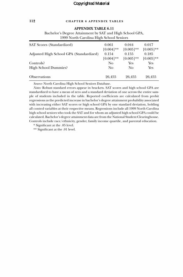
112 C H A P T E R 6 A P P E N D I X T A B L E S
APPENDIX TABLE 6.11Bachelor’s Degree Attainment by SAT and High School GPA,
1999 North Carolina High School Seniors
SAT Scores (Standardized) 0.061 0.044 0.017[0.004]** [0.005]** [0.005]**
Adjusted High School GPA (Standardized) 0.154 0.155 0.185[0.004]** [0.005]** [0.005]**
Controls? No Yes YesHigh School Dummies? No No Yes
Observations 26,455 26,455 26,455
Source: North Carolina High School Seniors Database.Notes: Robust standard errors appear in brackets. SAT scores and high school GPA are
standardized to have a mean of zero and a standard deviation of one across the entire sam-ple of students included in the table. Reported coefficients are calculated from probit regressions as the predicted increase in bachelor’s degree attainment probability associatedwith increasing either SAT scores or high school GPA by one standard deviation, holdingall control variables at their respective means. Regressions include all 1999 North Carolinahigh school seniors who took the SAT and for whom an adjusted high school GPA could becalculated. Bachelor’s degree attainment data are from the National Student Clearinghouse.Controls include race/ethnicity, gender, family income quartile, and parental education.
* Significant at the .05 level.** Significant at the .01 level.
Copyrighted MaterialCopyrighted MaterialCopyrighted Material
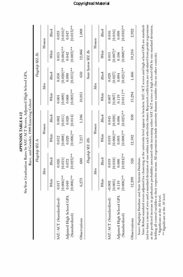
AP
PE
ND
IX T
AB
LE
6.1
2Si
x-Ye
ar G
radu
atio
n R
ates
by
SAT
/AC
T S
core
s, A
djus
ted
Hig
h S
choo
l GPA
, R
ace,
an
d G
ende
r, 19
99 E
nte
rin
g C
ohor
t
Flag
ship
SEL
Is
Flag
ship
SEL
IIs
Men
Wom
enM
enW
omen
Whi
teB
lack
Whi
teB
lack
Whi
teB
lack
Whi
teB
lack
SAT
/AC
T (
Stan
dard
ized
)0.
017
0.02
60.
012
0.00
20.
001
0.05
80.
015
0.03
3[0
.006
]**
[0.0
15]
[0.0
08]
[0.0
11]
[0.0
09]
[0.0
20]*
*[0
.004
]**
[0.0
16]*
Adj
uste
d H
igh
Sch
ool G
PA
0.04
90.
072
0.02
90.
020
0.06
80.
090
0.04
20.
047
(Sta
nda
rdiz
ed)
[0.0
06]*
*[0
.023
]**
[0.0
06]*
*[0
.014
][0
.003
]**
[0.0
15]*
*[0
.003
]**
[0.0
13]*
*
Obs
erva
tion
s6,
273
680
7,21
71,
106
10,9
511,
650
12,0
661,
008
Flag
ship
SEL
III
sSt
ate
Syst
em S
EL B
s
Men
Wom
enM
enW
omen
Whi
teB
lack
Whi
teB
lack
Whi
teB
lack
Whi
teB
lack
SAT
/AC
T (
Stan
dard
ized
)–0
.002
0.01
90.
019
0.04
50.
007
0.02
90.
015
0.01
6[0
.005
][0
.018
][0
.006
]**
[0.0
28]
[0.0
07]
[0.0
27]
[0.0
07]*
[0.0
16]
Adj
uste
d H
igh
Sch
ool G
PA
0.11
90.
080
0.09
30.
096
0.11
90.
094
0.10
60.
099
(Sta
nda
rdiz
ed)
[0.0
06]*
*[0
.024
]**
[0.0
08]*
*[0
.025
]**
[0.0
11]*
*[0
.021
]**
[0.0
08]*
*[0
.010
]**
Obs
erva
tion
s12
,299
526
12,1
821,
838
15,2
941,
466
19,2
162,
922
Sour
ce:F
lags
hip
s D
atab
ase
and
Stat
e Sy
stem
s D
atab
ase.
Not
es:R
obus
t sta
nda
rd e
rror
s ad
just
ed fo
r cl
uste
rin
g at
the
univ
ersi
ty le
vel a
ppea
r in
bra
cket
s. S
AT
/AC
T s
core
s an
d h
igh
sch
ool G
PA a
re s
tan
dard
-iz
ed to
hav
e a
mea
n o
f zer
o an
d a
stan
dard
dev
iati
on o
f on
e w
ith
in e
ach
sele
ctiv
ity
clus
ter.
Rep
orte
d co
effi
cien
ts a
re c
alcu
late
d fr
om p
robi
t reg
ress
ion
sas
the
pred
icte
d in
crea
se in
gra
duat
ion
pro
babi
lity
asso
ciat
ed w
ith
incr
easi
ng
eith
er S
AT
/AC
T s
core
s or
hig
h s
choo
l GPA
by
one
stan
dard
dev
iati
on,
hol
din
g al
l con
trol
var
iabl
es a
t th
eir
resp
ecti
ve m
ean
s. A
ll re
gres
sion
s in
clud
e un
iver
sity
dum
my
vari
able
s (b
ut n
o ot
her
con
trol
s).
* Si
gnifi
can
t at t
he
.05
leve
l.**
Sig
nifi
can
t at t
he
.01
leve
l.
Copyrighted MaterialCopyrighted MaterialCopyrighted Material

AP
PE
ND
IX T
AB
LE
6.1
3Si
x-Ye
ar G
radu
atio
n R
ates
by
SAT
/AC
T S
core
s, A
djus
ted
Hig
h S
choo
l GPA
, an
d Fa
mily
In
com
e Q
uart
ile, 1
999
En
teri
ng
Coh
ort
Flag
ship
SEL
Is
Flag
ship
SEL
IIs
Bot
tom
Seco
ndT
hird
Top
Bot
tom
Seco
ndT
hird
Top
SAT
/AC
T (
Stan
dard
ized
)0.
029
0.02
1–0
.006
0.00
90.
012
0.00
90.
012
0.00
1[0
.008
]**
[0.0
08]*
[0.0
07]
[0.0
04]*
[0.0
06]*
[0.0
10]
[0.0
06]
[0.0
04]
Adj
uste
d H
igh
Sch
ool G
PA
(Sta
nda
rdiz
ed)
0.04
70.
046
0.06
70.
036
0.08
90.
075
0.07
60.
056
[0.0
18]*
[0.0
09]*
*[0
.008
]**
[0.0
04]*
*[0
.012
]**
[0.0
06]*
*[0
.003
]**
[0.0
05]*
*
Obs
erva
tion
s2,
436
2,78
24,
456
10,9
403,
439
3,98
17,
774
14,1
40
Flag
ship
SEL
III
sSt
ate
Syst
em S
EL B
s
Bot
tom
Seco
ndT
hird
Top
Bot
tom
Seco
ndT
hird
Top
SAT
/AC
T (
Stan
dard
ized
)0.
023
0.00
10.
015
–0.0
050.
024
0.00
70.
003
–0.0
01[0
.016
][0
.012
][0
.006
]*[0
.006
][0
.011
]*[0
.010
][0
.008
][0
.007
]A
djus
ted
Hig
h S
choo
l GPA
(S
tan
dard
ized
)0.
111
0.12
80.
108
0.10
50.
111
0.11
30.
128
0.11
8[0
.008
]**
[0.0
08]*
*[0
.012
]**
[0.0
06]*
*[0
.007
]**
[0.0
09]*
*[0
.009
]**
[0.0
11]*
*
Obs
erva
tion
s4,
051
5,15
68,
491
10,5
595,
657
8,88
312
,442
11,5
51
Sour
ce:F
lags
hip
s D
atab
ase
and
Stat
e Sy
stem
s D
atab
ase.
Not
es:R
obus
t sta
nda
rd e
rror
s ad
just
ed fo
r cl
uste
rin
g at
the
univ
ersi
ty le
vel a
ppea
r in
bra
cket
s. S
AT
/AC
T s
core
s an
d h
igh
sch
ool G
PA a
re s
tan
dard
-iz
ed to
hav
e a
mea
n o
f zer
o an
d a
stan
dard
dev
iati
on o
f on
e w
ith
in e
ach
sele
ctiv
ity
clus
ter.
Rep
orte
d co
effi
cien
ts a
re c
alcu
late
d fr
om p
robi
t reg
ress
ion
sas
the
pred
icte
d in
crea
se in
gra
duat
ion
pro
babi
lity
asso
ciat
ed w
ith
incr
easi
ng
eith
er S
AT
/AC
T s
core
s or
hig
h s
choo
l GPA
by
one
stan
dard
dev
iati
on,
hol
din
g al
l con
trol
var
iabl
es a
t th
eir
resp
ecti
ve m
ean
s. A
ll re
gres
sion
s in
clud
e un
iver
sity
dum
my
vari
able
s (b
ut n
o ot
her
con
trol
var
iabl
es).
* Si
gnifi
can
t at t
he
.05
leve
l.**
Sig
nifi
can
t at t
he
.01
leve
l.
Copyrighted MaterialCopyrighted MaterialCopyrighted Material

C H A P T E R 6 A P P E N D I X T A B L E S 115
APPENDIX TABLE 6.14Six-Year Graduation Rates by SAT/ACT Scores, Adjusted High School GPA,
Race/Ethnicity, and Gender, 1999 Entering Cohort, Flagships
All Flagships
Men Women
White Black Hispanic White Black Hispanic
SAT/ACT (Standardized) 0.004 0.037 0.033 0.018 0.029 0.024[0.005] [0.012]** [0.009]** [0.003]** [0.011]** [0.009]**
Adjusted High School 0.092 0.092 0.077 0.064 0.058 0.057GPA (Standardized) [0.004]** [0.013]** [0.011]** [0.004]** [0.012]** [0.015]**
Observations 29,523 1,856 1,982 31,465 2,952 2,259
Source: Flagships Database.Notes: Robust standard errors adjusted for clustering at the university level appear in brackets. SAT/ACT
scores and high school GPA are standardized to have a mean of zero and a standard deviation of one acrossall flagships. Reported coefficients are calculated from probit regressions as the predicted increase in grad-uation probability associated with increasing either SAT/ACT scores or high school GPA by one standard de-viation, holding all control variables at their respective means. All regressions include university dummy vari-ables (but no other control variables).
* Significant at the .05 level.** Significant at the .01 level.
Copyrighted MaterialCopyrighted MaterialCopyrighted Material
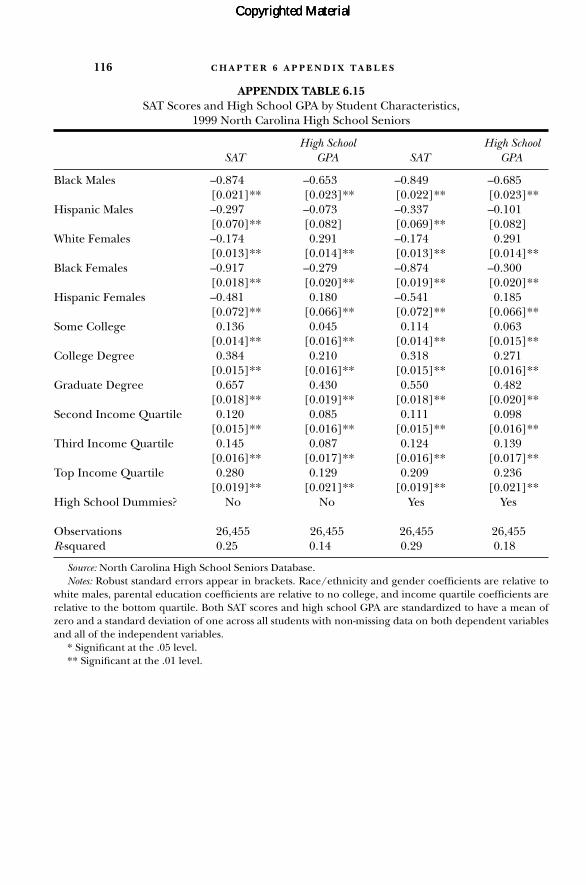
116 C H A P T E R 6 A P P E N D I X T A B L E S
APPENDIX TABLE 6.15SAT Scores and High School GPA by Student Characteristics,
1999 North Carolina High School Seniors
High School High SchoolSAT GPA SAT GPA
Black Males –0.874 –0.653 –0.849 –0.685[0.021]** [0.023]** [0.022]** [0.023]**
Hispanic Males –0.297 –0.073 –0.337 –0.101[0.070]** [0.082] [0.069]** [0.082]
White Females –0.174 0.291 –0.174 0.291[0.013]** [0.014]** [0.013]** [0.014]**
Black Females –0.917 –0.279 –0.874 –0.300[0.018]** [0.020]** [0.019]** [0.020]**
Hispanic Females –0.481 0.180 –0.541 0.185[0.072]** [0.066]** [0.072]** [0.066]**
Some College 0.136 0.045 0.114 0.063[0.014]** [0.016]** [0.014]** [0.015]**
College Degree 0.384 0.210 0.318 0.271[0.015]** [0.016]** [0.015]** [0.016]**
Graduate Degree 0.657 0.430 0.550 0.482[0.018]** [0.019]** [0.018]** [0.020]**
Second Income Quartile 0.120 0.085 0.111 0.098[0.015]** [0.016]** [0.015]** [0.016]**
Third Income Quartile 0.145 0.087 0.124 0.139[0.016]** [0.017]** [0.016]** [0.017]**
Top Income Quartile 0.280 0.129 0.209 0.236[0.019]** [0.021]** [0.019]** [0.021]**
High School Dummies? No No Yes Yes
Observations 26,455 26,455 26,455 26,455R-squared 0.25 0.14 0.29 0.18
Source: North Carolina High School Seniors Database.Notes: Robust standard errors appear in brackets. Race/ethnicity and gender coefficients are relative to
white males, parental education coefficients are relative to no college, and income quartile coefficients arerelative to the bottom quartile. Both SAT scores and high school GPA are standardized to have a mean ofzero and a standard deviation of one across all students with non-missing data on both dependent variablesand all of the independent variables.
* Significant at the .05 level.** Significant at the .01 level.
Copyrighted MaterialCopyrighted MaterialCopyrighted Material

AP
PE
ND
IX T
AB
LE
6.1
6R
ank-
in-C
lass
at E
xit b
y SA
T/A
CT
Sco
res
and
Adj
uste
d H
igh
Sch
ool G
PA, 1
999
En
teri
ng
Coh
ort,
Flag
ship
s
19 F
lags
hips
SEL
Is
SEL
IIs
SEL
III
s
SAT
/AC
T (
Stan
dard
ized
)7.
37.
24.
94.
75.
23.
54.
34.
83.
5[0
.8]*
*[0
.6]*
*[0
.4]*
*[0
.5]*
*[0
.7]*
*[0
.9]*
[0.8
]**
[0.7
]**
[0.8
]**
Adj
uste
d H
igh
Sch
ool G
PA
8.5
7.8
10.2
9.5
8.4
9.9
11.7
10.9
12.3
(Sta
nda
rdiz
ed)
[0.9
]**
[0.8
]**
[0.6
]**
[0.6
]**
[0.5
]**
[0.7
]**
[0.5
]**
[0.5
]**
[0.5
]**
Un
iver
sity
Dum
mie
s?Ye
sYe
sYe
sYe
sYe
sYe
sYe
sYe
sYe
sC
ontr
ols
Incl
uded
?N
oYe
sYe
sN
oYe
sYe
sN
oYe
sYe
sH
igh
Sch
ool D
umm
ies?
No
No
Yes
No
No
Yes
No
No
Yes
Obs
erva
tion
s20
,394
20,3
9420
,384
21,9
8421
,984
21,9
2928
,115
28,1
1528
,097
14 F
lags
hips
with
Par
enta
l Edu
catio
n D
ata
Ava
ilabl
e
SEL
Is
SEL
IIs
SEL
III
s
SAT
/AC
T (
Stan
dard
ized
)7.
46.
94.
84.
54.
62.
73.
74.
02.
7[0
.8]*
*[0
.5]*
*[0
.3]*
*[0
.6]*
[0.4
]**
[0.4
]*[1
.0]*
[0.9
]*[1
.0]
Adj
uste
d H
igh
Sch
ool G
PA
8.4
7.9
10.1
9.5
8.7
10.4
12.2
11.3
12.9
(Sta
nda
rdiz
ed)
[0.8
]**
[0.7
]**
[0.5
]**
[1.0
]*[0
.8]*
*[1
.2]*
[0.5
]**
[0.6
]**
[0.6
]**
Un
iver
sity
Dum
mie
s?Ye
sYe
sYe
sYe
sYe
sYe
sYe
sYe
sYe
sC
ontr
ols
Incl
uded
?N
oYe
sYe
sN
oYe
sYe
sN
oYe
sYe
sH
igh
Sch
ool D
umm
ies?
No
No
Yes
No
No
Yes
No
No
Yes
Obs
erva
tion
s19
,936
19,9
3619
,926
10,8
4010
,840
10,8
0115
,702
15,7
0215
,692
Sour
ce:F
lags
hip
s D
atab
ase.
Not
es:R
obus
t sta
nda
rd e
rror
s ad
just
ed fo
r cl
uste
rin
g at
the
univ
ersi
ty le
vel a
ppea
r in
bra
cket
s. S
AT
/AC
T s
core
s an
d h
igh
sch
ool G
PA a
re s
tan
dard
-iz
ed to
hav
e a
mea
n o
f zer
o an
d a
stan
dard
dev
iati
on o
f on
e w
ith
in e
ach
sel
ecti
vity
clu
ster
. Obs
erva
tion
s w
ith
mis
sin
g va
lues
on
an
y of
the
con
trol
var
i-ab
les
are
excl
uded
. Con
trol
var
iabl
es a
re s
tate
res
iden
cy s
tatu
s, r
ace/
eth
nic
ity,
gen
der,
and
fam
ily in
com
e qu
arti
le. T
he
bott
om p
anel
als
o in
clud
espa
ren
tal e
duca
tion
as
a co
ntr
ol v
aria
ble.
* Si
gnifi
can
t at t
he
.05
leve
l.**
Sig
nifi
can
t at t
he
.01
leve
l.
Copyrighted MaterialCopyrighted MaterialCopyrighted Material
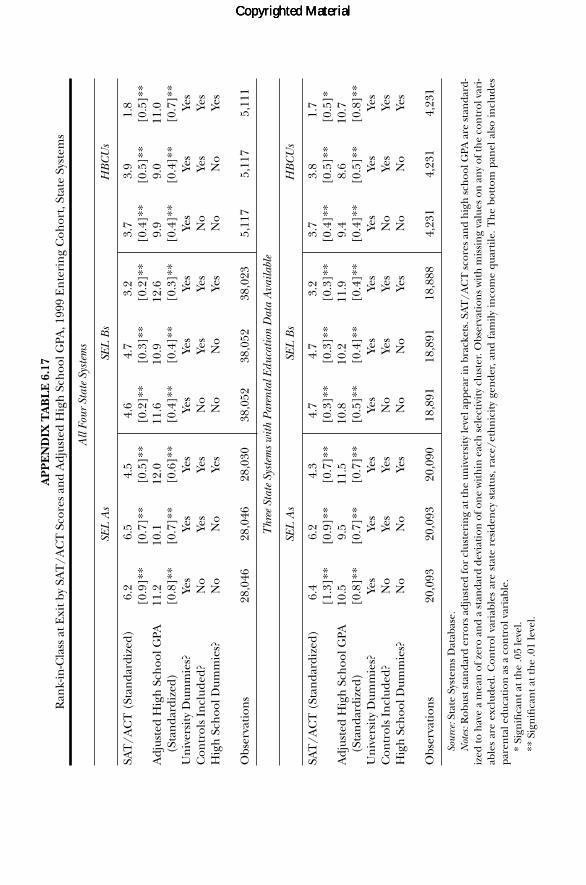
AP
PE
ND
IX T
AB
LE
6.1
7R
ank-
in-C
lass
at E
xit b
y SA
T/A
CT
Sco
res
and
Adj
uste
d H
igh
Sch
ool G
PA, 1
999
En
teri
ng
Coh
ort,
Stat
e Sy
stem
s
All
Four
Sta
te S
yste
ms
SEL
As
SEL
Bs
HB
CU
s
SAT
/AC
T (
Stan
dard
ized
)6.
26.
54.
54.
64.
73.
23.
73.
91.
8[0
.9]*
*[0
.7]*
*[0
.5]*
*[0
.2]*
*[0
.3]*
*[0
.2]*
*[0
.4]*
*[0
.5]*
*[0
.5]*
*A
djus
ted
Hig
h S
choo
l GPA
11
.210
.112
.011
.610
.912
.69.
99.
011
.0(S
tan
dard
ized
)[0
.8]*
*[0
.7]*
*[0
.6]*
*[0
.4]*
*[0
.4]*
*[0
.3]*
*[0
.4]*
*[0
.4]*
*[0
.7]*
*U
niv
ersi
ty D
umm
ies?
Yes
Yes
Yes
Yes
Yes
Yes
Yes
Yes
Yes
Con
trol
s In
clud
ed?
No
Yes
Yes
No
Yes
Yes
No
Yes
Yes
Hig
h S
choo
l Dum
mie
s?N
oN
oYe
sN
oN
oYe
sN
oN
oYe
s
Obs
erva
tion
s28
,046
28,0
4628
,030
38,0
5238
,052
38,0
235,
117
5,11
75,
111
Thr
ee S
tate
Sys
tem
s w
ith P
aren
tal E
duca
tion
Dat
a A
vaila
ble
SEL
As
SEL
Bs
HB
CU
s
SAT
/AC
T (
Stan
dard
ized
)6.
46.
24.
34.
74.
73.
23.
73.
81.
7[1
.3]*
*[0
.9]*
*[0
.7]*
*[0
.3]*
*[0
.3]*
*[0
.3]*
*[0
.4]*
*[0
.5]*
*[0
.5]*
Adj
uste
d H
igh
Sch
ool G
PA
10.5
9.5
11.5
10.8
10.2
11.9
9.4
8.6
10.7
(Sta
nda
rdiz
ed)
[0.8
]**
[0.7
]**
[0.7
]**
[0.5
]**
[0.4
]**
[0.4
]**
[0.4
]**
[0.5
]**
[0.8
]**
Un
iver
sity
Dum
mie
s?Ye
sYe
sYe
sYe
sYe
sYe
sYe
sYe
sYe
sC
ontr
ols
Incl
uded
?N
oYe
sYe
sN
oYe
sYe
sN
oYe
sYe
sH
igh
Sch
ool D
umm
ies?
No
No
Yes
No
No
Yes
No
No
Yes
Obs
erva
tion
s20
,093
20,0
9320
,090
18,8
9118
,891
18,8
884,
231
4,23
14,
231
Sour
ce:S
tate
Sys
tem
s D
atab
ase.
Not
es:R
obus
t sta
nda
rd e
rror
s ad
just
ed fo
r cl
uste
rin
g at
the
univ
ersi
ty le
vel a
ppea
r in
bra
cket
s. S
AT
/AC
T s
core
s an
d h
igh
sch
ool G
PA a
re s
tan
dard
-iz
ed to
hav
e a
mea
n o
f zer
o an
d a
stan
dard
dev
iati
on o
f on
e w
ith
in e
ach
sel
ecti
vity
clu
ster
. Obs
erva
tion
s w
ith
mis
sin
g va
lues
on
an
y of
the
con
trol
var
i-ab
les
are
excl
uded
. Con
trol
var
iabl
es a
re s
tate
res
iden
cy s
tatu
s, r
ace/
eth
nic
ity
gen
der,
and
fam
ily i
nco
me
quar
tile
. Th
e bo
ttom
pan
el a
lso
incl
udes
pare
nta
l edu
cati
on a
s a
con
trol
var
iabl
e.*
Sign
ifica
nt a
t th
e .0
5 le
vel.
** S
ign
ifica
nt a
t th
e .0
1 le
vel.
Copyrighted MaterialCopyrighted MaterialCopyrighted Material

C H A P T E R 6 A P P E N D I X T A B L E S 119
APPENDIX TABLE 6.18Graduation Rates by SAT/ACT Scores, High School GPA, and Average of SAT II Scores,
1999 Entering Cohort
Six-Year Graduation Rates
Flagship SEL Is State System SEL As
SAT/ACT (Standardized) 0.018 0.014 0.002 0.010 0.002 0.000[0.003]** [0.002]** [0.003] [0.005]* [0.007] [0.007]
Adjusted High School GPA 0.045 0.035 0.034 0.061 0.042 0.042(Standardized) [0.004]** [0.004]** [0.003]** [0.003]** [0.004]** [0.004]**
Average of SAT II Scores 0.015 0.002(Standardized) [0.004]** [0.006]
Sample Restricted? No Yes Yes No Yes Yes
Observations 21,923 14,074 14,074 23,324 11,431 11,431
Four-Year Graduation Rates
Flagship SEL Is State System SEL As
SAT/ACT (Standardized) 0.043 0.038 0.017 0.009 –0.002 –0.022[0.004]** [0.006]** [0.004]** [0.014] [0.015] [0.019]
Adjusted High School GPA 0.074 0.064 0.061 0.099 0.081 0.078(Standardized) [0.006]** [0.007]** [0.007]** [0.010]** [0.008]** [0.009]**
Average of SAT II Scores 0.028 0.027(Standardized) [0.009]** [0.008]**
Sample Restricted? No Yes Yes No Yes Yes
Observations 21,923 14,074 14,074 23,324 11,431 11,431
Source: Flagships Database and State Systems Database.Notes: Robust standard errors adjusted for clustering at the university level appear in brackets. SAT/ACT
scores, high school GPA, and average SAT II scores are standardized to have a mean of zero and a standarddeviation of one within each selectivity cluster, and the standardization is done separately for the set of ob-servations in each regression. All regressions include university dummies. “Sample Restricted” indicates thatstudents who did not take an SAT II exam are excluded.
* Significant at the .05 level.** Significant at the .01 level.
Copyrighted MaterialCopyrighted MaterialCopyrighted Material
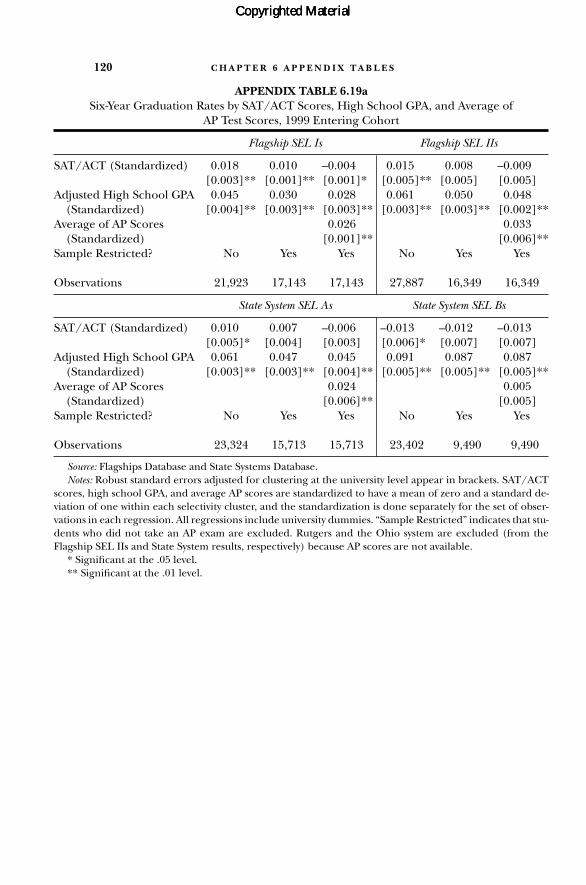
120 C H A P T E R 6 A P P E N D I X T A B L E S
APPENDIX TABLE 6.19aSix-Year Graduation Rates by SAT/ACT Scores, High School GPA, and Average of
AP Test Scores, 1999 Entering Cohort
Flagship SEL Is Flagship SEL IIs
SAT/ACT (Standardized) 0.018 0.010 –0.004 0.015 0.008 –0.009[0.003]** [0.001]** [0.001]* [0.005]** [0.005] [0.005]
Adjusted High School GPA 0.045 0.030 0.028 0.061 0.050 0.048(Standardized) [0.004]** [0.003]** [0.003]** [0.003]** [0.003]** [0.002]**
Average of AP Scores 0.026 0.033(Standardized) [0.001]** [0.006]**
Sample Restricted? No Yes Yes No Yes Yes
Observations 21,923 17,143 17,143 27,887 16,349 16,349
State System SEL As State System SEL Bs
SAT/ACT (Standardized) 0.010 0.007 –0.006 –0.013 –0.012 –0.013[0.005]* [0.004] [0.003] [0.006]* [0.007] [0.007]
Adjusted High School GPA 0.061 0.047 0.045 0.091 0.087 0.087(Standardized) [0.003]** [0.003]** [0.004]** [0.005]** [0.005]** [0.005]**
Average of AP Scores 0.024 0.005(Standardized) [0.006]** [0.005]
Sample Restricted? No Yes Yes No Yes Yes
Observations 23,324 15,713 15,713 23,402 9,490 9,490
Source: Flagships Database and State Systems Database.Notes: Robust standard errors adjusted for clustering at the university level appear in brackets. SAT/ACT
scores, high school GPA, and average AP scores are standardized to have a mean of zero and a standard de-viation of one within each selectivity cluster, and the standardization is done separately for the set of obser-vations in each regression. All regressions include university dummies. “Sample Restricted” indicates that stu-dents who did not take an AP exam are excluded. Rutgers and the Ohio system are excluded (from theFlagship SEL IIs and State System results, respectively) because AP scores are not available.
* Significant at the .05 level.** Significant at the .01 level.
Copyrighted MaterialCopyrighted MaterialCopyrighted Material
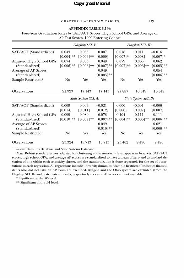
C H A P T E R 6 A P P E N D I X T A B L E S 121
APPENDIX TABLE 6.19bFour-Year Graduation Rates by SAT/ACT Scores, High School GPA, and Average of
AP Test Scores, 1999 Entering Cohort
Flagship SEL Is Flagship SEL IIs
SAT/ACT (Standardized) 0.043 0.033 0.007 0.018 0.011 –0.016[0.004]** [0.006]** [0.009] [0.007]* [0.008] [0.007]*
Adjusted High School GPA 0.074 0.053 0.049 0.079 0.065 0.062(Standardized) [0.006]** [0.006]** [0.007]** [0.007]** [0.006]** [0.005]**
Average of AP Scores 0.049 0.054(Standardized) [0.005]** [0.006]**
Sample Restricted? No Yes Yes No Yes Yes
Observations 21,923 17,143 17,143 27,887 16,349 16,349
State System SEL As State System SEL Bs
SAT/ACT (Standardized) 0.009 0.004 –0.021 0.000 –0.001 –0.006[0.014] [0.011] [0.012] [0.006] [0.007] [0.007]
Adjusted High School GPA 0.099 0.080 0.078 0.104 0.111 0.111(Standardized) [0.010]** [0.007]** [0.007]** [0.004]** [0.006]** [0.006]**
Average of AP Scores 0.049 0.021(Standardized) [0.010]** [0.006]**
Sample Restricted? No Yes Yes No Yes Yes
Observations 23,324 15,713 15,713 23,402 9,490 9,490
Source: Flagships Database and State Systems Database.Notes: Robust standard errors adjusted for clustering at the university level appear in brackets. SAT/ACT
scores, high school GPA, and average AP scores are standardized to have a mean of zero and a standard de-viation of one within each selectivity cluster, and the standardization is done separately for the set of obser-vations in each regression. All regressions include university dummies. “Sample Restricted” indicates that stu-dents who did not take an AP exam are excluded. Rutgers and the Ohio system are excluded (from theFlagship SEL IIs and State System results, respectively) because AP scores are not available.
* Significant at the .05 level.** Significant at the .01 level.
Copyrighted MaterialCopyrighted MaterialCopyrighted Material

AP
PE
ND
IX T
AB
LE
7.1
aTr
ansf
er A
dmis
sion
s at
Fla
gsh
ips
and
Stat
e Sy
stem
SE
L A
s
Adm
itFr
omFr
omR
ate
Num
ber
%Tw
o-Ye
ar
Four
-Yea
rU
nive
rsity
App
lied
Adm
itted
(%)
Enro
lled
Tran
sfer
s(%
)(%
)
Iow
a St
ate
Un
iver
sity
2,88
82,
283
791,
655
2953
47N
orth
Car
olin
a St
ate
Un
iver
sity
2,94
81,
547
521,
035
2330
70O
hio
Sta
te U
niv
ersi
ty4,
728
3,18
267
1,71
522
Rut
gers
, Th
e St
ate
Un
iver
sity
of N
ew J
erse
y6,
360
2,44
438
1,24
619
Ston
y B
rook
Un
iver
sity
–SU
NY
4,18
32,
603
621,
432
37U
niv
ersi
ty o
f Cal
ifor
nia
–Ber
kele
y7,
750
2,37
131
1,60
631
8911
Un
iver
sity
of C
alif
orn
ia–L
os A
nge
les
10,3
503,
796
372,
268
3592
8U
niv
ersi
ty o
f Flo
rida
5,23
82,
374
451,
845
3378
22U
niv
ersi
ty o
f Illi
noi
s at
Urb
ana-
Ch
ampa
ign
2,57
61,
382
541,
066
1467
33U
niv
ersi
ty o
f Iow
a3,
107
2,04
066
1,31
825
6040
Un
iver
sity
of M
D–B
alti
mor
e C
oun
ty1,
907
1,58
583
1,06
843
6644
Un
iver
sity
of M
aryl
and–
Col
lege
Par
k4,
813
3,37
970
2,18
136
5347
Un
iver
sity
of N
ebra
ska–
Lin
coln
1,48
31,
149
7791
620
4852
Un
iver
sity
of N
orth
Car
olin
a–C
hap
el H
ill1,
868
1,04
056
712
1725
75U
niv
ersi
ty o
f Nor
th C
arol
ina–
Ash
evill
e62
943
369
287
3850
50U
niv
ersi
ty o
f Ore
gon
2,34
21,
983
851,
371
3530
70U
niv
ersi
ty o
f Tex
as–A
usti
n6,
649
3,12
847
2,03
822
5446
Un
iver
sity
of V
irgi
nia
2,22
179
136
540
1634
66U
niv
ersi
ty o
f Wis
con
sin
–Mad
ison
3,08
01,
773
581,
138
1723
77
Sour
ce:C
olle
ge B
oard
An
nua
l Sur
vey
of C
olle
ges.
Not
es: “
Perc
ent
Tran
sfer
s” is
th
e n
umbe
r of
en
teri
ng
tran
sfer
s di
vide
d by
th
e to
tal n
umbe
r of
en
teri
ng
stud
ents
(tr
ansf
ers
and
fres
hm
en).
All
data
desc
ribe
th
e 19
99 e
nte
rin
g cl
ass,
wit
h t
he
follo
win
g ex
cept
ion
s (a
nd
the
ente
rin
g cl
ass
desc
ribe
d n
oted
in p
aren
thes
es):
all
data
fro
m R
utge
rs U
ni-
vers
ity
and
the
Un
iver
sity
of C
alif
orn
ia–L
os A
nge
les (
2000
); p
erce
nta
ge o
f tra
nsf
ers a
t Sto
ny
Bro
ok U
niv
ersi
ty a
nd
the
Un
iver
sity
of W
isco
nsi
n–M
adis
on(2
000)
; an
d pe
rcen
tage
from
two-
an
d fo
ur-y
ear
colle
ges a
t th
e U
niv
ersi
ty o
f Illi
noi
s at U
rban
a-C
ham
paig
n (
2003
), th
e U
niv
ersi
ty o
f Neb
rask
a–L
inco
ln(2
000)
, an
d th
e U
niv
ersi
ty o
f Nor
th C
arol
ina–
Ch
apel
Hill
(20
03).
Copyrighted MaterialCopyrighted MaterialCopyrighted Material
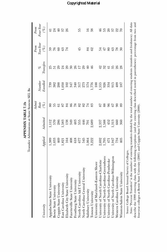
AP
PE
ND
IX T
AB
LE
7.1
bTr
ansf
er A
dmis
sion
s at
Sta
te S
yste
m S
EL
Bs
Adm
itFr
omFr
omR
ate
Num
ber
%Tw
o-Ye
ar
Four
-Yea
rU
nive
rsity
App
lied
Adm
itted
(%)
Enro
lled
Tran
sfer
s(%
)(%
)
App
alac
hia
n S
tate
Un
iver
sity
1,38
91,
112
8073
925
5941
Bow
ie S
tate
Un
iver
sity
1,03
357
055
382
5176
24C
oppi
n S
tate
Un
iver
sity
469
286
6120
029
6040
Eas
t Car
olin
a U
niv
ersi
ty1,
821
1,58
387
1,05
024
6337
Eliz
abet
h C
ity
Stat
e U
niv
ersi
ty16
413
884
102
2074
26Fa
yett
evill
e St
ate
Un
iver
sity
408
349
8634
730
Fros
tbur
g St
ate
Un
iver
sity
618
483
7834
026
Nor
th C
arol
ina
A&
T U
niv
ersi
ty67
755
582
317
1745
55N
orth
Car
olin
a C
entr
al U
niv
ersi
ty54
544
682
273
29Sa
lisbu
ry U
niv
ersi
ty1,
064
791
7457
440
8416
Tow
son
Un
iver
sity
3,22
22,
689
831,
776
4662
38U
niv
ersi
ty o
f Mar
ylan
d–E
aste
rn S
hor
e10
0U
niv
ersi
ty o
f Nor
th C
arol
ina–
Ch
arlo
tte
2,69
22,
337
871,
555
4254
46U
niv
ersi
ty o
f Nor
th C
arol
ina–
Gre
ensb
oro
1,79
51,
588
8892
632
4753
Un
iver
sity
of N
orth
Car
olin
a–Pe
mbr
oke
471
452
9633
441
8020
Un
iver
sity
of N
orth
Car
olin
a–W
ilmin
gton
1,94
71,
313
6791
535
6337
Wes
tern
Car
olin
a U
niv
ersi
ty73
466
090
409
2678
22W
inst
on-S
alem
Sta
te U
niv
ersi
ty40
536
089
187
2830
70
Sour
ce:C
olle
ge B
oard
An
nua
l Sur
vey
of C
olle
ges.
Not
es:“
Perc
ent
Tran
sfer
s” is
th
e n
umbe
r of
en
teri
ng
tran
sfer
s di
vide
d by
th
e to
tal n
umbe
r of
en
teri
ng
stud
ents
(tr
ansf
ers
and
fres
hm
en).
All
data
desc
ribe
th
e 19
99 e
nte
rin
g cl
ass,
wit
h t
he
follo
win
g ex
cept
ion
s (a
nd
the
ente
rin
g cl
ass
desc
ribe
d n
oted
in
par
enth
eses
): p
erce
nta
ge f
rom
tw
o- a
nd
four
-yea
r co
llege
s at
Bow
ie S
tate
Un
iver
sity
(20
01)
and
Cop
pin
Sta
te U
niv
ersi
ty (
2000
).
Copyrighted MaterialCopyrighted MaterialCopyrighted Material

124 C H A P T E R 7 A P P E N D I X T A B L E S
APPENDIX TABLE 7.3Bachelor’s Degree Attainment Rates of Transfer Students (Relative to Freshmen),
1999 Entering Cohort
Flagships and State System SEL As State System SEL Bs
Transfers from 0.007 0.001 0.081 0.089 0.082 0.136Two-Year [0.018] [0.014] [0.010]** [0.013]** [0.011]** [0.012]**
Transfers from 0.010 0.026 0.071 0.108 0.110 0.130Four-Year [0.016] [0.012]* [0.009]** [0.016]** [0.011]** [0.006]**
University No Yes Yes No Yes YesDummies?
High School GPA No No Yes No No Yesand SAT/ACT?
Observations 76,806 76,806 76,806 18,141 18,141 18,141
Source: Flagships Database and State Systems Database.Notes: Robust standard errors adjusted for clustering by university appear in brackets. Coefficients are mar-
ginal effects from a probit model and indicate the predicted difference in attaining a bachelor’s degree be-tween the listed group and the reference group (freshmen), holding any control variables at their means.“Attaining a bachelor’s degree” is defined as either graduating from the original institution or earning a de-gree from a later institution (if it is reported in the Clearinghouse degree data).
* Significant at the .05 level.** Significant at the .01 level.
APPENDIX TABLE 7.2Characteristics of Freshmen and Transfers, 1999 Entering Cohort
Flagships and State System SEL As State System SEL Bs
Freshmen Transfers 2 Transfers 4 Freshmen Transfers 2 Transfers 4
Number 70,621 8,542 7,236 16,488 2,871 1,753High School GPA 3.69 3.21 3.37 3.35 2.97 3.24SAT/ACT Scores 1177 1032 1100 1024 938 1009Age 18.4 20.8 20.3 18.4 20.7 20.5% White 72.1 73.2 78.6 83.1 89.3 81.6% Black 6.7 4.4 6.3 10.8 5.8 14.1% Hispanic 5.7 6.5 3.9 1.5 1.3 1.5% Asian 13.4 13.2 8.8 2.6 2.4 1.5
Source: Flagships Database and State Systems Database.Notes: “Transfers 2” is transfers from two-year institutions, and “Transfers 4” is transfers from four-year
institutions.
Copyrighted MaterialCopyrighted MaterialCopyrighted Material
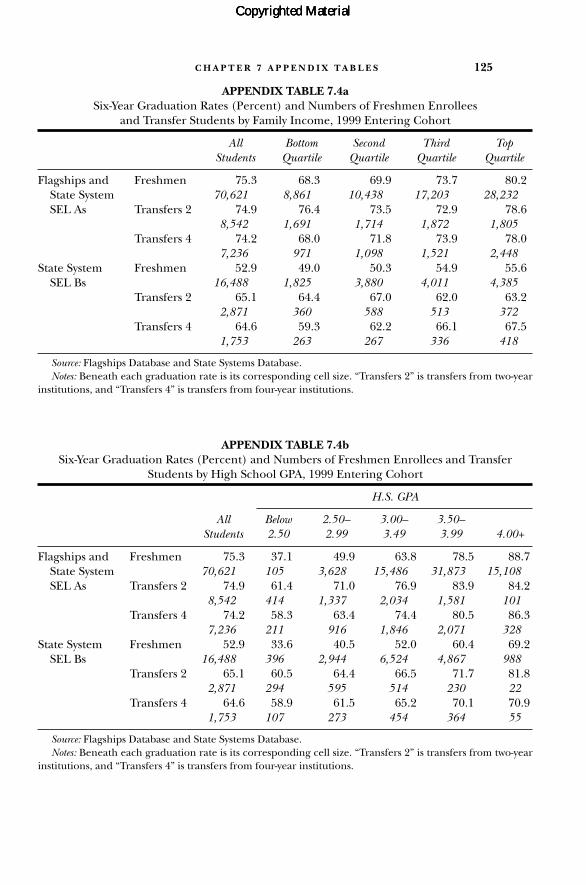
APPENDIX TABLE 7.4aSix-Year Graduation Rates (Percent) and Numbers of Freshmen Enrollees
and Transfer Students by Family Income, 1999 Entering Cohort
All Bottom Second Third TopStudents Quartile Quartile Quartile Quartile
Flagships and Freshmen 75.3 68.3 69.9 73.7 80.2State System 70,621 8,861 10,438 17,203 28,232SEL As Transfers 2 74.9 76.4 73.5 72.9 78.6
8,542 1,691 1,714 1,872 1,805Transfers 4 74.2 68.0 71.8 73.9 78.0
7,236 971 1,098 1,521 2,448State System Freshmen 52.9 49.0 50.3 54.9 55.6
SEL Bs 16,488 1,825 3,880 4,011 4,385Transfers 2 65.1 64.4 67.0 62.0 63.2
2,871 360 588 513 372Transfers 4 64.6 59.3 62.2 66.1 67.5
1,753 263 267 336 418
Source: Flagships Database and State Systems Database.Notes: Beneath each graduation rate is its corresponding cell size. “Transfers 2” is transfers from two-year
institutions, and “Transfers 4” is transfers from four-year institutions.
APPENDIX TABLE 7.4bSix-Year Graduation Rates (Percent) and Numbers of Freshmen Enrollees and Transfer
Students by High School GPA, 1999 Entering Cohort
H.S. GPA
All Below 2.50– 3.00– 3.50–Students 2.50 2.99 3.49 3.99 4.00+
Flagships and Freshmen 75.3 37.1 49.9 63.8 78.5 88.7State System 70,621 105 3,628 15,486 31,873 15,108SEL As Transfers 2 74.9 61.4 71.0 76.9 83.9 84.2
8,542 414 1,337 2,034 1,581 101Transfers 4 74.2 58.3 63.4 74.4 80.5 86.3
7,236 211 916 1,846 2,071 328State System Freshmen 52.9 33.6 40.5 52.0 60.4 69.2
SEL Bs 16,488 396 2,944 6,524 4,867 988Transfers 2 65.1 60.5 64.4 66.5 71.7 81.8
2,871 294 595 514 230 22Transfers 4 64.6 58.9 61.5 65.2 70.1 70.9
1,753 107 273 454 364 55
Source: Flagships Database and State Systems Database.Notes: Beneath each graduation rate is its corresponding cell size. “Transfers 2” is transfers from two-year
institutions, and “Transfers 4” is transfers from four-year institutions.
C H A P T E R 7 A P P E N D I X T A B L E S 125
Copyrighted MaterialCopyrighted MaterialCopyrighted Material

126 C H A P T E R 7 A P P E N D I X T A B L E S
APPENDIX TABLE 7.4cSix-Year Graduation Rates (Percent) of Freshmen Enrollees and Transfer Students
by SAT/ACT Scores, 1999 Entering Cohort
SAT/ACT
All Below 900– 1000– 1100–Students 900 990 1090 1190 1200+
Flagships and Freshmen 75.3 57.5 63.8 69.3 74.5 82.0State System 70,621 2,736 6,665 11,321 17,127 31,916SEL As Transfers 2 74.9 69.3 75.0 78.0 77.4 79.3
8,542 1,195 1,522 1,442 1,299 944Transfers 4 74.2 62.4 72.1 75.0 77.6 79.3
7,236 651 1,075 1,351 1,540 1,776State System Freshmen 52.9 47.7 51.7 54.4 55.7 57.7
SEL Bs 16,488 2,750 4,127 4,652 2,966 1,811Transfers 2 65.1 66.1 64.6 65.1 68.6 58.7
2,871 601 438 307 137 63Transfers 4 64.6 63.3 64.5 65.2 66.2 73.9
1,753 283 304 299 234 134
Source: Flagships Database and State Systems Database.Notes: Beneath each graduation rate is its corresponding cell size. “Transfers 2” is transfers from two-year
institutions, and “Transfers 4” is transfers from four-year institutions.
APPENDIX TABLE 7.5Major at Graduation of Freshmen Enrollees and Transfer Students
(Percentage of Students in Each Field), 1999 Entering Cohort
Flagships and State System SEL As State System SEL Bs
Transfers Transfers Transfers TransfersFreshmen 2 4 Freshmen 2 4
Engineering, Math, 20 15 14 8 9 7and Physical Sciences
Life Sciences 9 8 8 4 3 6Humanities 11 13 14 13 11 11Social Sciences 23 29 27 15 14 17Communications and 11 10 11 21 23 17
EducationBusiness 14 11 11 23 23 22Professional and Other 12 14 14 17 17 19
Source: Flagships Database and State Systems Database.Notes: “Transfers 2” is transfers from two-year institutions, and “Transfers 4” is transfers from four-year
institutions.
Copyrighted MaterialCopyrighted MaterialCopyrighted Material

APPENDIX TABLE 7.6Rank-in-Class at Graduation of Transfer Students (Relative to Freshmen),
1999 Entering Cohort
Flagships and State System SEL As State System SEL Bs
Transfers from –10.6 –10.5 9.4 –5.2 –5.2 9.2Two-Year [1.1]** [1.0]** [1.4]** [1.7]* [1.7]* [1.0]**
Transfers from –3.4 –3.2 7.2 0.7 1.2 5.4Four-Year [0.8]** [0.8]** [0.9]** [1.9] [1.7] [0.9]**
University No Yes Yes No Yes Yesand Major?
High School GPA No No Yes No No Yesand SAT/ACT?
Observations 50,531 50,531 50,531 9,954 9,954 9,954
Source: Flagships Database and State Systems Database.Notes: Robust standard errors adjusted for clustering by university appear in brackets. Coefficients indicate
the average difference in rank-in-class at graduation between the listed group and the reference group (fresh-men enrollees).
* Significant at the .05 level.** Significant at the .01 level.
C H A P T E R 7 A P P E N D I X T A B L E S 127
Copyrighted MaterialCopyrighted MaterialCopyrighted Material

128 C H A P T E R 7 A P P E N D I X T A B L E S
APPENDIX TABLE 7.7aAverage Rank-in-Class at Graduation of Freshmen Enrollees and Transfer Students
by High School GPA, 1999 Entering Cohort
High School GPA
All Below 2.50– 3.00– 3.50–Students 2.50 2.99 3.49 3.99 4.00+
Flagships and Freshmen 51.1 20.2 27.6 38.4 52.4 62.0State System 44,602 31 1,615 8,451 21,854 11,402SEL As Transfers 2 41.3 27.2 30.5 40.5 51.0 51.6
5,508 253 910 1,479 1,211 76Transfers 4 47.5 27.0 32.4 42.7 56.9 68.6
4,367 119 546 1,256 1,470 217State System Freshmen 50.8 32.1 34.2 44.2 59.8 77.1
SEL Bs 8,716 133 1,193 3,392 2,938 684Transfers 2 45.9 33.7 39.5 49.1 64.5 67.9
1,868 178 383 342 165 18Transfers 4 51.6 24.8 38.8 49.5 65.1 79.2
1,133 63 168 296 255 39
Source: Flagships Database and State Systems Database.Notes: Beneath each average rank is its corresponding cell size. “Transfers 2” is transfers from two-year in-
stitutions, and “Transfers 4” is transfers from four-year institutions.
APPENDIX TABLE 7.7bAverage Rank-in-Class at Graduation of Freshmen Enrollees and Transfer Students
by SAT/ACT Scores, 1999 Entering Cohort
SAT/ACT
All Below 900– 1000– 1100–Students 900 990 1090 1190 1200+
Flagships and Freshmen 51.1 27.8 36.4 42.7 48.9 58.6State System 44,602 1,365 3,693 6,464 10,736 22,177SEL As Transfers 2 41.3 29.1 37.7 40.7 44.9 52.5
5,508 748 1,004 968 893 686Transfers 4 47.5 29.2 37.3 44.5 50.8 59.2
4,367 367 665 835 1,006 1,151State System Freshmen 50.8 37.2 43.9 50.7 58.5 69.8
SEL Bs 8,716 1,311 2,133 2,530 1,652 1,045Transfers 2 45.9 36.9 46.4 48.8 60.9 70.5
1,868 397 283 200 94 37Transfers 4 51.6 35.5 44.1 56.2 63.6 67.2
1,133 179 196 195 155 99
Source: Flagships Database and State Systems Database.Notes: Beneath each average rank is its corresponding cell size. “Transfers 2” is transfers from two-year in-
stitutions, and “Transfers 4” is transfers from four-year institutions.
Copyrighted MaterialCopyrighted MaterialCopyrighted Material

C H A P T E R 7 A P P E N D I X T A B L E S 129
APPENDIX TABLE 7.8Academic Predictors of Transfers’ College Outcomes, 1999 Entering Cohort
Transfers from Two-Year Schools
Graduation Rate Rank-in-Class
Standardized Transfer GPA 0.069 0.065 15.5 13.7[0.008]** [0.010]** [0.7]** [0.9]**
Standardized Adjusted High School GPA 0.018 2.6[0.010] [0.8]*
Standardized SAT/ACT Score –0.012 2.3[0.006]* [0.4]**
Observations 3,145 3,145 3,138 3,138
Transfers from Four-Year Schools
Graduation Rate Rank-in-Class
Standardized Transfer GPA 0.062 0.054 15.8 12.8[0.010]** [0.009]** [1.3]** [1.3]**
Standardized Adjusted High School GPA 0.033 5.6[0.009]** [1.4]**
Standardized SAT/ACT Score –0.011 4.2[0.008] [0.6]**
Observations 2,268 2,268 2,268 2,268
Source: Flagships Database.Notes: Robust standard errors adjusted for clustering within universities appear in brackets. “Graduation
Rate” is six-year graduation status, and “Rank-in-Class” is measured at exit. SAT/ACT scores, transfer GPA,and adjusted high school GPA are all standardized to have a mean of zero and a standard deviation of oneso that the coefficients on these variables can be compared. All regressions include institutional dummies.This table is based on data from only eight flagship universities: Iowa State University, the University of California–Berkeley and –Los Angeles, the University of Illinois at Urbana-Champaign, the University ofNorth Carolina–Chapel Hill, and the Universities of Iowa, Maryland, and Oregon, because the transfer GPAis available only at these universities.
* Significant at the .05 level.** Significant at the .01 level.
Copyrighted MaterialCopyrighted MaterialCopyrighted Material

130 C H A P T E R 7 A P P E N D I X T A B L E S
APPENDIX TABLE 7.9Comparison of Predictors for Freshmen Enrollees versus Transfers, 1999 Entering Cohort
Flagships and State System SEL As
Six-Year Graduation Rates Rank-in-Class at Exit
Transfers Transfers Transfers TransfersFreshmen 2 4 Freshmen 2 4
Standardized 0.084 0.040 0.062 12.1 6.1 8.5 Adjusted High [0.004]** [0.008]** [0.011]** [0.6]** [0.7]** [0.7]**School GPA
Standardized 0.015 –0.012 –0.004 6.1 4.1 5.1SAT/ACT [0.003]** [0.007] [0.005] [0.6]** [0.5]** [0.5]**Score
Observations 57,056 5,040 4,829 57,056 5,040 4,829
State System SEL Bs
Six-Year Graduation Rates Rank-in-Class at Exit
Transfers Transfers Transfers TransfersFreshmen 2 4 Freshmen 2 4
Standardized 0.087 0.045 0.046 10.9 6.7 7.9Adjusted High [0.004]** [0.012]** [0.020]* [0.5]** [0.6]** [1.3]**School GPA
Standardized –0.013 –0.022 0.011 4.7 4.5 5.3SAT/ACT [0.007] [0.011]* [0.012] [0.3]** [0.5]** [0.5]**Score
Observations 15,547 1,436 1,166 15,547 1,436 1,166
Source: Flagships Database and State Systems Database.Notes: Robust standard errors in brackets. SAT/ACT scores and adjusted high school GPA are both stan-
dardized to have a mean of zero and a standard deviation of one so that the coefficients on these variablescan be compared. All regressions include institutional dummies. Rutgers is excluded because high schoolGPA is not available for any transfer students.
* Significant at the .05 level.** Significant at the .01 level.
Copyrighted MaterialCopyrighted MaterialCopyrighted Material

C H A P T E R 7 A P P E N D I X T A B L E S 131
APPENDIX TABLE 7.11Outcomes and Characteristics of Freshmen Enrollees and Transfer Students
with High School GPAs below 3.0, 1999 Entering Cohort
Number Grad % Rank % Bot Y % Top Y
Flagships and Freshmen 3,733 50 27.5 17 38State System Transfers 2 1,751 69 29.8 19 30SEL As Transfers 4 1,127 62 31.4 18 40
State System Freshmen 3,340 40 34.0 10 39SEL Bs Transfers 2 889 63 37.6 16 28
Transfers 4 380 61 35.0 18 37
Source: Flagships Database and State Systems Database.Notes: “Transfers 2” is transfers from two-year institutions, and “Transfers 4” is transfers from four-year in-
stitutions. “Grad %” is six-year graduation rate. “Rank” is rank-in-class at graduation. “% Bot Y” and “% TopY” are the percentages of students in the bottom and top income quartiles, respectively.
APPENDIX TABLE 7.10Outcomes and Characteristics of Freshmen Enrollees and Transfers
at HBCUs, 1999 Entering Cohort
Freshmen Transfers 2 Transfers 4
Number 5,045 276 322Graduation Rate (%) 39.7 53.3 52.2Rank-in-Class 49.5 49.5 54.4High School GPA 2.96 2.72 2.84SAT/ACT Scores 847 806 866
Source: State Systems Database.Notes: Data are from HBCUs in Maryland and North Carolina. “Transfer 2” is transfers
from two-year institutions, and “Transfers 4” is transfers from four-year institutions.
APPENDIX TABLE 7.12Educational Attainment of the Population Aged 25–34 by State, 2000
(Percentage in Each Category)
Some College, Bachelor’s DegreeState No Degree Associate’s Degree or Higher
Massachusetts 18 8 41Connecticut 20 7 35Colorado 24 8 35New Jersey 20 7 35Minnesota 27 11 35Maryland 23 6 34New York 18 9 33
(continued )
Copyrighted MaterialCopyrighted MaterialCopyrighted Material
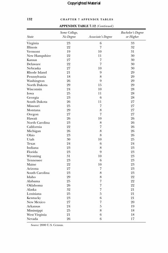
132 C H A P T E R 7 A P P E N D I X T A B L E S
APPENDIX TABLE 7.12 (Continued)
Some College, Bachelor’s DegreeState No Degree Associate’s Degree or Higher
Virginia 23 6 33Illinois 22 7 32Vermont 19 10 31New Hampshire 22 11 30Kansas 27 7 30Delaware 22 7 30Nebraska 27 10 30Rhode Island 21 9 29Pennsylvania 18 8 29Washington 26 9 29North Dakota 29 15 29Wisconsin 24 10 28Iowa 25 11 28Georgia 23 6 28South Dakota 26 11 27Missouri 25 7 27Montana 29 8 27Oregon 27 7 27Hawaii 26 10 26North Carolina 23 8 26California 22 7 26Michigan 26 8 26Ohio 23 8 26Utah 30 10 25Texas 24 6 24Indiana 23 8 23Florida 23 9 23Wyoming 31 10 23Tennessee 23 6 23Maine 22 10 23Arizona 27 7 23South Carolina 23 8 23Idaho 29 8 22Alabama 25 7 22Oklahoma 26 7 22Alaska 32 7 21Louisiana 25 5 21Kentucky 23 6 21New Mexico 27 7 20Arkansas 24 5 19Mississippi 25 8 18West Virginia 21 6 18Nevada 26 6 17
Source: 2000 U.S. Census.
Copyrighted MaterialCopyrighted MaterialCopyrighted Material

C H A P T E R 8 A P P E N D I X T A B L E S 133
APPENDIX TABLE 8.1Average Tuition and Fees (Constant 2008 Dollars) and Percent Change,
1978–79 to 2008–09
Public Four-Year InstitutionsPrivate Four-Year Institutions (In-state Rates)
Published Year-to-Year Published Year-to-YearAcademic Tuition Change Tuition ChangeYear and Fees (%) and Fees (%)
1978–79 9,903 — 2,303 —1979–80 9,704 –2.1 2,221 –3.71980–81 9,620 –0.9 2,138 –3.81981–82 9,877 2.6 2,183 2.01982–83 10,466 5.6 2,326 6.21983–84 11,214 6.7 2,528 8.01984–85 11,740 4.5 2,595 2.61985–86 12,490 6.0 2,689 3.51986–87 13,375 6.6 2,840 5.31987–88 13,623 1.8 2,870 1.01988–89 14,857 8.3 2,929 2.01989–90 15,318 3.0 2,999 2.31990–91 15,755 2.8 3,218 6.81991–92 15,846 0.6 3,403 5.41992–93 16,357 3.1 3,654 6.91993–94 16,767 2.4 3,862 5.41994–95 17,370 3.5 4,009 3.71995–96 17,620 1.4 4,055 1.11996–97 18,205 3.2 4,168 2.71997–98 18,892 3.6 4,264 2.21998–99 19,825 4.7 4,376 2.61999–2000 20,476 3.2 4,436 1.32000–2001 20,459 –0.1 4,465 0.72001–02 21,534 5.0 4,667 4.32002–03 22,057 2.4 5,005 6.82003–04 22,666 2.7 5,556 9.92004–05 23,280 2.6 5,953 6.72005–06 23,617 1.4 6,182 3.72006–07 24,113 2.1 6,274 1.52007–08 25,075 3.8 6,538 4.02008–09 25,143 0.3 6,585 0.7
Source: Trends in College Pricing (College Board 1999, 2008a) and authors’ calculations.Note: “—” indicates that the change from the previous year cannot be calculated because
data from the previous year are not available.
Copyrighted MaterialCopyrighted MaterialCopyrighted Material

AP
PE
ND
IX T
AB
LE
8.2
Ave
rage
Per
cen
t Ch
ange
in P
ublis
hed
an
d N
et T
uiti
on (
Con
stan
t 200
8 D
olla
rs),
199
3–94
to 2
008–
09
Priv
ate
Four
-Yea
r In
stitu
tions
Publ
ic F
our-Y
ear
Inst
itutio
ns
Publ
ishe
dA
vera
gePu
blis
hed
Year
-to-Y
ear
Ave
rage
Year
-to-Y
ear
(In-
stat
e)Ye
ar-to
-Yea
r(I
n-st
ate)
Year
-to-Y
ear
Tuiti
onPe
rcen
tN
et T
uitio
nPe
rcen
tTu
ition
Perc
ent
Net
Tui
tion
Perc
ent
Aca
dem
ic Y
ear
and
Fees
Cha
nge
and
Fees
Cha
nge
and
Fees
Cha
nge
and
Fees
Cha
nge
1993
–94
16,8
00—
10,6
00—
3,90
0—
2,30
0—
1994
–95
17,4
003.
410
,700
0.9
4,00
02.
52,
200
–4.5
1995
–96
17,6
001.
110
,800
0.9
4,10
02.
42,
100
–4.8
1996
–97
18,2
003.
311
,300
4.4
4,20
02.
42,
200
4.5
1997
–98
18,9
003.
711
,800
4.2
4,30
02.
32,
200
0.0
1998
–99
19,8
004.
512
,200
3.3
4,40
02.
32,
200
0.0
1999
–200
020
,500
3.4
12,7
003.
94,
400
0.0
2,20
00.
020
00–2
001
20,5
000.
012
,600
–0.8
4,50
02.
22,
100
–4.8
2001
–02
21,5
004.
713
,500
6.7
4,70
04.
32,
000
–5.0
2002
–03
22,1
002.
713
,800
2.2
5,00
06.
02,
200
9.1
2003
–04
22,7
002.
613
,900
0.7
5,60
010
.72,
100
–4.8
2004
–05
23,3
002.
614
,300
2.8
6,00
06.
72,
400
12.5
2005
–06
23,6
001.
314
,400
0.7
6,20
03.
22,
700
11.1
2006
–07
24,1
002.
114
,600
1.4
6,30
01.
62,
700
2.1
2007
–08
25,1
004.
015
,100
3.3
6,50
03.
12,
800
3.6
2008
–09
25,1
000.
014
,900
–1.3
6,60
01.
52,
900
3.4
Sour
ce:T
rend
s in
Col
lege
Pri
cing
(Col
lege
Boa
rd 1
999,
200
8a)
and
auth
ors’
cal
cula
tion
s.N
ote:
“—”
indi
cate
s th
at th
e ch
ange
from
the
prev
ious
yea
r ca
nn
ot b
e ca
lcul
ated
bec
ause
dat
a fr
om th
e pr
evio
us y
ear
are
not
ava
ilabl
e.
Copyrighted MaterialCopyrighted MaterialCopyrighted Material
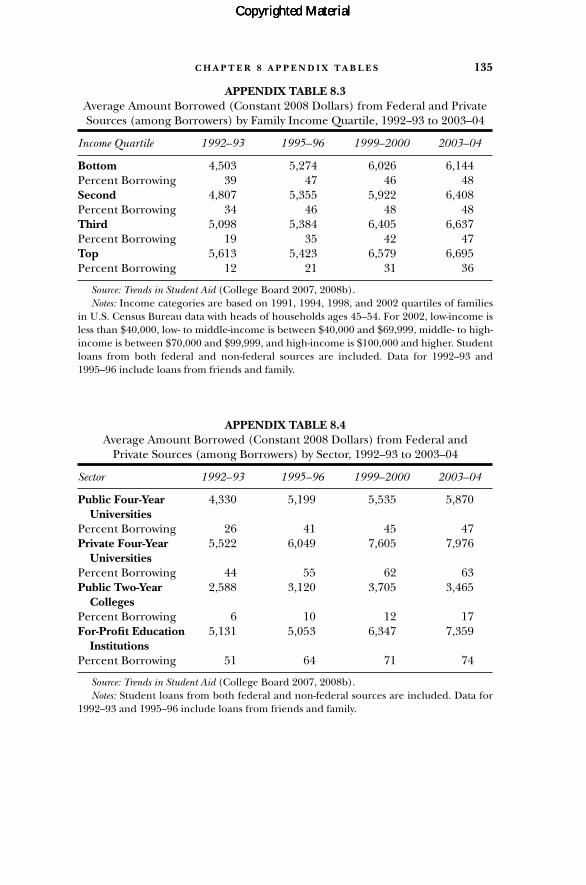
C H A P T E R 8 A P P E N D I X T A B L E S 135
APPENDIX TABLE 8.3Average Amount Borrowed (Constant 2008 Dollars) from Federal and PrivateSources (among Borrowers) by Family Income Quartile, 1992–93 to 2003–04
Income Quartile 1992–93 1995–96 1999–2000 2003–04
Bottom 4,503 5,274 6,026 6,144Percent Borrowing 39 47 46 48Second 4,807 5,355 5,922 6,408Percent Borrowing 34 46 48 48Third 5,098 5,384 6,405 6,637Percent Borrowing 19 35 42 47Top 5,613 5,423 6,579 6,695Percent Borrowing 12 21 31 36
Source: Trends in Student Aid (College Board 2007, 2008b).Notes: Income categories are based on 1991, 1994, 1998, and 2002 quartiles of families
in U.S. Census Bureau data with heads of households ages 45–54. For 2002, low-income isless than $40,000, low- to middle-income is between $40,000 and $69,999, middle- to high-income is between $70,000 and $99,999, and high-income is $100,000 and higher. Studentloans from both federal and non-federal sources are included. Data for 1992–93 and1995–96 include loans from friends and family.
APPENDIX TABLE 8.4Average Amount Borrowed (Constant 2008 Dollars) from Federal and
Private Sources (among Borrowers) by Sector, 1992–93 to 2003–04
Sector 1992–93 1995–96 1999–2000 2003–04
Public Four-Year 4,330 5,199 5,535 5,870Universities
Percent Borrowing 26 41 45 47Private Four-Year 5,522 6,049 7,605 7,976
UniversitiesPercent Borrowing 44 55 62 63Public Two-Year 2,588 3,120 3,705 3,465
CollegesPercent Borrowing 6 10 12 17For-Profit Education 5,131 5,053 6,347 7,359
InstitutionsPercent Borrowing 51 64 71 74
Source: Trends in Student Aid (College Board 2007, 2008b).Notes: Student loans from both federal and non-federal sources are included. Data for
1992–93 and 1995–96 include loans from friends and family.
Copyrighted MaterialCopyrighted MaterialCopyrighted Material

AP
PE
ND
IX T
AB
LE
9.1
aA
vera
ge F
inan
cial
Aid
Pac
kage
s (1
999
Dol
lars
) by
Rac
e/E
thn
icit
y an
d Fa
mily
In
com
e,
1999
En
teri
ng
Coh
ort,
Flag
ship
s an
d St
ate
Syst
em S
EL
As
Tota
l Gra
nts
All
Rac
es/
Inco
me
Qua
rtile
Ethn
iciti
esW
hite
Bla
ckH
ispa
nic
Asi
anO
ther
Rac
es
Bot
tom
Qua
rtile
6,53
95,
705
7,66
07,
801
7,23
06,
433
Perc
ent R
ecei
vin
g G
ran
ts92
9095
9692
95Se
cond
Qua
rtile
4,34
83,
919
5,71
05,
667
5,12
34,
101
Perc
ent R
ecei
vin
g G
ran
ts81
7989
8781
87T
hird
Qua
rtile
2,93
72,
749
4,00
23,
922
3,44
02,
383
Perc
ent R
ecei
vin
g G
ran
ts55
5470
6747
74T
op Q
uart
ile2,
783
2,60
24,
450
3,88
33,
176
1,60
8Pe
rcen
t Rec
eivi
ng
Gra
nts
3535
5151
2465
Tota
l Loa
ns
All
Rac
es/
Inco
me
Qua
rtile
Ethn
iciti
esW
hite
Bla
ckH
ispa
nic
Asi
anO
ther
Rac
es
Bot
tom
Qua
rtile
3,30
23,
516
3,17
12,
983
2,97
62,
506
Perc
ent B
orro
win
g60
6161
6456
81Se
cond
Qua
rtile
4,14
44,
288
3,95
83,
473
3,64
42,
884
Perc
ent B
orro
win
g61
6264
6254
75T
hird
Qua
rtile
5,02
85,
057
5,12
24,
809
4,76
63,
530
Perc
ent B
orro
win
g48
4956
5039
68T
op Q
uart
ile5,
331
5,33
95,
378
4,94
65,
335
2,56
6Pe
rcen
t Bor
row
ing
2323
3626
1856
Copyrighted MaterialCopyrighted MaterialCopyrighted Material
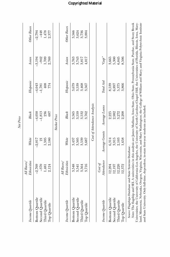
Net
Pri
ce
All
Rac
es/
Inco
me
Qua
rtile
Ethn
iciti
esW
hite
Bla
ckH
ispa
nic
Asi
anO
ther
Rac
es
Bot
tom
Qua
rtile
–2,7
69–2
,017
–4,0
50–4
,043
–3,1
94–2
,794
Seco
nd
Qua
rtile
–370
21–1
,813
–1,7
81–9
42–4
48T
hir
d Q
uart
ile1,
481
1,59
523
640
81,
709
1,47
8To
p Q
uart
ile2,
124
2,18
069
777
42,
769
2,37
7
Stic
ker
Pric
e
All
Rac
es/
Inco
me
Qua
rtile
Ethn
iciti
esW
hite
Bla
ckH
ispa
nic
Asi
anO
ther
Rac
es
Bot
tom
Qua
rtile
3,54
83,
437
3,56
53,
679
3,76
33,
566
Seco
nd
Qua
rtile
3,54
13,
505
3,55
93,
539
3,74
33,
624
Th
ird
Qua
rtile
3,56
43,
539
3,53
23,
468
3,81
73,
736
Top
Qua
rtile
3,71
63,
687
3,76
23,
567
4,01
73,
884
Cos
t of A
ttend
ance
Ana
lysi
s
Cos
t of
Inco
me
Qua
rtile
Atte
ndan
ceA
vera
ge G
rant
sA
vera
ge L
oans
Tota
l Aid
“Gap
”
Bot
tom
Qua
rtile
12,2
046,
314
2,22
58,
539
3,66
5Se
con
d Q
uart
ile12
,197
3,91
52,
982
6,89
75,
300
Th
ird
Qua
rtile
12,2
202,
103
3,27
25,
375
6,84
5To
p Q
uart
ile12
,372
1,65
82,
208
3,86
68,
506
Sour
ce:F
lags
hip
s D
atab
ase
and
Stat
e Sy
stem
s D
atab
ase.
Not
es:T
he
flag
ship
an
d SE
L A
un
iver
siti
es in
this
an
alys
is a
re J
ames
Mad
ison
, Iow
a St
ate,
Oh
io S
tate
, Pen
nsy
lvan
ia S
tate
, Pur
due,
an
d St
ony
Bro
okU
niv
ersi
ties
; th
e U
niv
ersi
ty o
f C
alif
orn
ia–L
os A
nge
les,
th
e U
niv
ersi
ty o
f N
orth
Car
olin
a–C
hap
el H
ill, t
he
Un
iver
siti
es o
f Fl
orid
a, I
llin
ois,
Iow
a, M
ary-
lan
d, M
inn
esot
a, N
ebra
ska,
Ore
gon
, Vir
gin
ia, W
isco
nsi
n, a
nd
Mar
y W
ash
ingt
on; t
he
Col
lege
of
Will
iam
an
d M
ary;
an
d V
irgi
nia
Pol
ytec
hn
ic I
nst
itut
ean
d St
ate
Un
iver
sity
. On
ly fu
ll-ti
me,
dep
ende
nt,
in-s
tate
firs
t-yea
r st
uden
ts a
re in
clud
ed.
Copyrighted MaterialCopyrighted MaterialCopyrighted Material
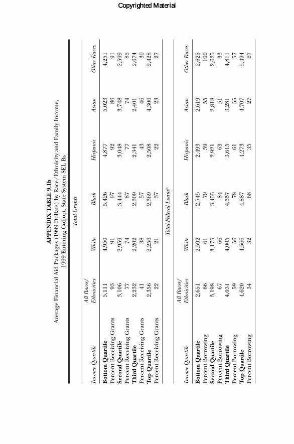
AP
PE
ND
IX T
AB
LE
9.1
bA
vera
ge F
inan
cial
Aid
Pac
kage
s (1
999
Dol
lars
) by
Rac
e/E
thn
icit
y an
d Fa
mily
In
com
e,19
99 E
nte
rin
g C
ohor
t, St
ate
Syst
em S
EL
Bs
Tota
l Gra
nts
All
Rac
es/
Inco
me
Qua
rtile
Ethn
iciti
esW
hite
Bla
ckH
ispa
nic
Asi
anO
ther
Rac
es
Bot
tom
Qua
rtile
5,11
14,
950
5,42
64,
877
5,02
34,
251
Perc
ent R
ecei
vin
g G
ran
ts93
9197
9286
91Se
cond
Qua
rtile
3,10
62,
959
3,44
43,
048
3,74
82,
599
Perc
ent R
ecei
vin
g G
ran
ts77
7487
7774
85T
hird
Qua
rtile
2,23
22,
202
2,30
92,
341
2,40
12,
674
Perc
ent R
ecei
vin
g G
ran
ts41
3857
4346
30T
op Q
uart
ile2,
356
2,25
62,
369
2,50
84,
306
2,42
8Pe
rcen
t Rec
eivi
ng
Gra
nts
2221
3722
2327
Tota
l Fed
eral
Loa
nsa
All
Rac
es/
Inco
me
Qua
rtile
Ethn
iciti
esW
hite
Bla
ckH
ispa
nic
Asi
anO
ther
Rac
es
Bot
tom
Qua
rtile
2,65
12,
592
2,74
52,
493
2,61
92,
625
Perc
ent B
orro
win
g66
6179
5955
100
Seco
nd Q
uart
ile3,
198
3,17
53,
455
2,92
12,
818
2,62
5Pe
rcen
t Bor
row
ing
6766
8463
5133
Thi
rd Q
uart
ile4,
031
4,00
54,
557
3,61
53,
281
4,81
1Pe
rcen
t Bor
row
ing
5956
7861
5557
Top
Qua
rtile
4,62
04,
566
4,88
74,
273
4,70
75,
494
Perc
ent B
orro
win
g34
3268
3527
67
Copyrighted MaterialCopyrighted MaterialCopyrighted Material

Net
Pri
ce
All
Rac
es/
Inco
me
Qua
rtile
Ethn
iciti
esW
hite
Bla
ckH
ispa
nic
Asi
anO
ther
Rac
es
Bot
tom
Qua
rtile
–2,2
13–2
,100
–2,6
12–1
,676
–1,5
67–2
,141
Seco
nd
Qua
rtile
–347
–254
–693
130
–338
–624
Th
ird
Qua
rtile
1,28
31,
248
1,19
81,
755
1,89
028
3To
p Q
uart
ile1,
660
1,63
61,
740
2,14
91,
773
671
Stic
ker
Pric
e
All
Rac
es/
Inco
me
Qua
rtile
Ethn
iciti
esW
hite
Bla
ckH
ispa
nic
Asi
anO
ther
Rac
es
Bot
tom
Qua
rtile
2,81
52,
753
2,78
43,
101
3,23
32,
106
Seco
nd
Qua
rtile
2,56
52,
512
2,58
82,
893
3,09
01,
954
Th
ird
Qua
rtile
2,65
42,
596
2,83
13,
075
3,24
92,
183
Top
Qua
rtile
2,68
32,
634
2,83
53,
148
3,38
72,
254
Sour
ce:S
tate
Sys
tem
s D
atab
ase.
Not
es:B
ased
on
dat
a fr
om A
ppal
ach
ian
an
d E
ast C
arol
ina
Un
iver
siti
es; t
he
Un
iver
sity
of N
orth
Car
olin
a at
Ch
arlo
tte,
Gre
ensb
oro,
Wilm
ingt
on, a
nd
Pem
brok
e; C
hri
stop
her
New
port
, Geo
rge
Mas
on, L
ongw
ood,
Old
Dom
inio
n, R
adfo
rd, a
nd
Vir
gin
ia C
omm
onw
ealt
h U
niv
ersi
ties
; th
e U
niv
ersi
ty o
f Vir
-gi
nia
Col
lege
–Wis
e; a
nd
Vir
gin
ia M
ilita
ry A
cade
my.
On
ly fu
ll-ti
me,
dep
ende
nt,
in-s
tate
fres
hm
en a
re in
clud
ed.
aE
xcep
t “To
tal F
eder
al L
oan
s,”
wh
ich
is b
ased
on
ly o
n th
e ei
ght V
irgi
nia
inst
itut
ion
s. S
ee C
hap
ter
9, n
ote
8.
Copyrighted MaterialCopyrighted MaterialCopyrighted Material
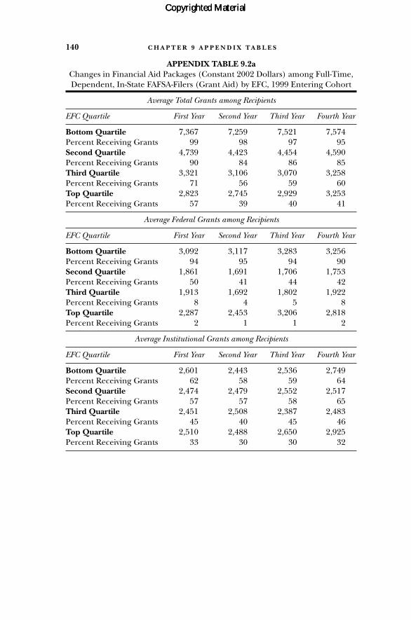
140 C H A P T E R 9 A P P E N D I X T A B L E S
APPENDIX TABLE 9.2aChanges in Financial Aid Packages (Constant 2002 Dollars) among Full-Time,Dependent, In-State FAFSA-Filers (Grant Aid) by EFC, 1999 Entering Cohort
Average Total Grants among Recipients
EFC Quartile First Year Second Year Third Year Fourth Year
Bottom Quartile 7,367 7,259 7,521 7,574Percent Receiving Grants 99 98 97 95Second Quartile 4,739 4,423 4,454 4,590Percent Receiving Grants 90 84 86 85Third Quartile 3,321 3,106 3,070 3,258Percent Receiving Grants 71 56 59 60Top Quartile 2,823 2,745 2,929 3,253Percent Receiving Grants 57 39 40 41
Average Federal Grants among Recipients
EFC Quartile First Year Second Year Third Year Fourth Year
Bottom Quartile 3,092 3,117 3,283 3,256Percent Receiving Grants 94 95 94 90Second Quartile 1,861 1,691 1,706 1,753Percent Receiving Grants 50 41 44 42Third Quartile 1,913 1,692 1,802 1,922Percent Receiving Grants 8 4 5 8Top Quartile 2,287 2,453 3,206 2,818Percent Receiving Grants 2 1 1 2
Average Institutional Grants among Recipients
EFC Quartile First Year Second Year Third Year Fourth Year
Bottom Quartile 2,601 2,443 2,536 2,749Percent Receiving Grants 62 58 59 64Second Quartile 2,474 2,479 2,552 2,517Percent Receiving Grants 57 57 58 65Third Quartile 2,451 2,508 2,387 2,483Percent Receiving Grants 45 40 45 46Top Quartile 2,510 2,488 2,650 2,925Percent Receiving Grants 33 30 30 32
Copyrighted MaterialCopyrighted MaterialCopyrighted Material
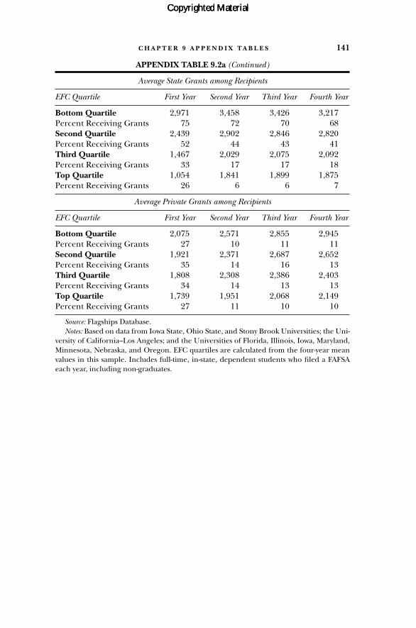
C H A P T E R 9 A P P E N D I X T A B L E S 141
APPENDIX TABLE 9.2a (Continued)
Average State Grants among Recipients
EFC Quartile First Year Second Year Third Year Fourth Year
Bottom Quartile 2,971 3,458 3,426 3,217Percent Receiving Grants 75 72 70 68Second Quartile 2,439 2,902 2,846 2,820Percent Receiving Grants 52 44 43 41Third Quartile 1,467 2,029 2,075 2,092Percent Receiving Grants 33 17 17 18Top Quartile 1,054 1,841 1,899 1,875Percent Receiving Grants 26 6 6 7
Average Private Grants among Recipients
EFC Quartile First Year Second Year Third Year Fourth Year
Bottom Quartile 2,075 2,571 2,855 2,945Percent Receiving Grants 27 10 11 11Second Quartile 1,921 2,371 2,687 2,652Percent Receiving Grants 35 14 16 13Third Quartile 1,808 2,308 2,386 2,403Percent Receiving Grants 34 14 13 13Top Quartile 1,739 1,951 2,068 2,149Percent Receiving Grants 27 11 10 10
Source: Flagships Database.Notes: Based on data from Iowa State, Ohio State, and Stony Brook Universities; the Uni-
versity of California–Los Angeles; and the Universities of Florida, Illinois, Iowa, Maryland,Minnesota, Nebraska, and Oregon. EFC quartiles are calculated from the four-year meanvalues in this sample. Includes full-time, in-state, dependent students who filed a FAFSAeach year, including non-graduates.
Copyrighted MaterialCopyrighted MaterialCopyrighted Material

142 C H A P T E R 9 A P P E N D I X T A B L E S
APPENDIX TABLE 9.2bChanges in Financial Aid Packages (Constant 2002 Dollars) among Full-Time,Dependent, In-State FAFSA-Filers (Loan Aid) by EFC, 1999 Entering Cohort
Average Total Loans among Borrowers
EFC Quartile First Year Second Year Third Year Fourth Year
Bottom Quartile 3,617 4,009 4,674 5,173Percent Borrowing 69 71 72 71Second Quartile 4,825 5,104 5,883 6,290Percent Borrowing 72 75 75 74Third Quartile 5,722 5,978 6,799 7,146Percent Borrowing 74 78 80 79Top Quartile 6,553 6,886 7,661 7,967Percent Borrowing 72 75 78 78
Average Federal Loans among Borrowers
EFC Quartile First Year Second Year Third Year Fourth Year
Bottom Quartile 3,460 3,806 4,490 4,977Percent Borrowing 69 71 72 71Second Quartile 4,357 4,555 5,443 5,718Percent Borrowing 72 74 75 74Third Quartile 5,124 5,219 6,165 6,406Percent Borrowing 74 77 79 78Top Quartile 6,047 6,289 7,068 7,300Percent Borrowing 72 74 78 78
Average Institutional Loans among Borrowers
EFC Quartile First Year Second Year Third Year Fourth Year
Bottom Quartile 1,801 2,049 2,603 1,573Percent Borrowing 0 0 0 0Second Quartile 1,602 1,760 1,647 2,150Percent Borrowing 3 2 1 1Third Quartile 1,436 1,912 1,609 2,165Percent Borrowing 2 2 1 1Top Quartile 1,445 2,696 3,797 1,737Percent Borrowing 1 0 0 0
Copyrighted MaterialCopyrighted MaterialCopyrighted Material
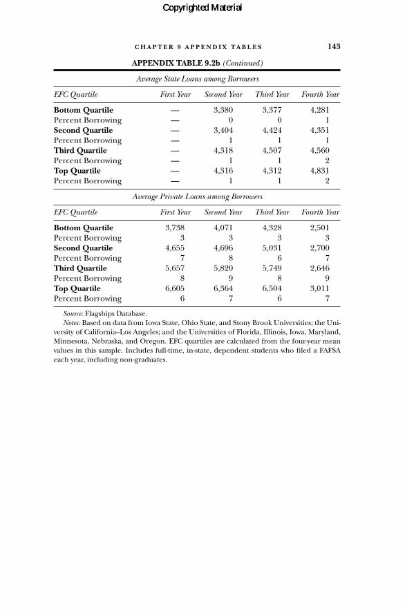
C H A P T E R 9 A P P E N D I X T A B L E S 143
APPENDIX TABLE 9.2b (Continued)
Average State Loans among Borrowers
EFC Quartile First Year Second Year Third Year Fourth Year
Bottom Quartile — 3,380 3,377 4,281Percent Borrowing — 0 0 1Second Quartile — 3,404 4,424 4,351Percent Borrowing — 1 1 1Third Quartile — 4,318 4,507 4,560Percent Borrowing — 1 1 2Top Quartile — 4,316 4,312 4,831Percent Borrowing — 1 1 2
Average Private Loans among Borrowers
EFC Quartile First Year Second Year Third Year Fourth Year
Bottom Quartile 3,738 4,071 4,328 2,501Percent Borrowing 3 3 3 3Second Quartile 4,655 4,696 5,031 2,700Percent Borrowing 7 8 6 7Third Quartile 5,657 5,820 5,749 2,646Percent Borrowing 8 9 8 9Top Quartile 6,605 6,364 6,504 3,011Percent Borrowing 6 7 6 7
Source: Flagships Database.Notes: Based on data from Iowa State, Ohio State, and Stony Brook Universities; the Uni-
versity of California–Los Angeles; and the Universities of Florida, Illinois, Iowa, Maryland,Minnesota, Nebraska, and Oregon. EFC quartiles are calculated from the four-year meanvalues in this sample. Includes full-time, in-state, dependent students who filed a FAFSAeach year, including non-graduates.
Copyrighted MaterialCopyrighted MaterialCopyrighted Material

AP
PE
ND
IX T
AB
LE
9.2
cC
han
ges
in F
amily
In
com
e, T
uiti
on, a
nd
EFC
(C
onst
ant 2
002
Dol
lars
) am
ong
Full-
Tim
e,
Dep
ende
nt,
In-S
tate
FA
FSA
-File
rs, 1
999
En
teri
ng
Coh
ort
Ave
rage
Fam
ily I
ncom
eA
vera
ge E
FC
EFC
Fi
rst
Seco
ndT
hird
Four
thEF
CFi
rst
Seco
ndT
hird
Four
thQ
uart
ileYe
arYe
arYe
arYe
arQ
uart
ileYe
arYe
arYe
arYe
ar
Bot
tom
Qua
rtile
22,8
6020
,289
20,3
0820
,996
Bot
tom
Qua
rtile
826
649
720
791
Seco
nd
Qua
rtile
45,4
9943
,473
44,5
2145
,287
Seco
nd
Qua
rtile
4,22
63,
566
3,71
53,
936
Th
ird
Qua
rtile
66,9
3467
,032
68,7
5868
,370
Th
ird
Qua
rtile
9,00
68,
597
8,86
18,
776
Top
Qua
rtile
101,
638
103,
809
106,
997
105,
592
Top
Qua
rtile
21,0
5422
,655
22,6
3920
,965
Ave
rage
Tui
tion
Ave
rage
Net
Tui
tion
EFC
Fi
rst
Seco
ndT
hird
Four
thEF
CFi
rst
Seco
ndT
hird
Four
thQ
uart
ileYe
arYe
arYe
arYe
arQ
uart
ileYe
arYe
arYe
arYe
ar
Bot
tom
Qua
rtile
3,59
54,
032
4,34
14,
776
Bot
tom
Qua
rtile
–3,7
14–3
,098
–2,9
37–2
,423
Seco
nd
Qua
rtile
3,51
63,
981
4,35
74,
862
Seco
nd
Qua
rtile
–740
284
524
973
Th
ird
Qua
rtile
3,56
53,
989
4,41
04,
935
Th
ird
Qua
rtile
1,21
12,
258
2,58
62,
965
Top
Qua
rtile
3,65
44,
169
4,58
15,
093
Top
Qua
rtile
2,05
03,
086
3,40
93,
749
Sour
ce:F
lags
hip
s D
atab
ase.
Not
es:B
ased
on
dat
a fr
om I
owa
Stat
e, O
hio
Sta
te, a
nd
Ston
y B
rook
Un
iver
siti
es; t
he
Un
iver
sity
of
Cal
ifor
nia
–Los
An
gele
s; a
nd
the
Un
iver
siti
es o
fFl
orid
a, I
llin
ois,
Iow
a, M
aryl
and,
Min
nes
ota,
Neb
rask
a, a
nd
Ore
gon
. EFC
qua
rtile
s ar
e ca
lcul
ated
fro
m t
he
four
-yea
r m
ean
val
ues
in t
his
sam
ple.
In
-cl
udes
full-
tim
e, in
-sta
te, d
epen
den
t stu
den
ts w
ho
file
d a
FAFS
A e
ach
yea
r, in
clud
ing
non
-gra
duat
es.
Copyrighted MaterialCopyrighted MaterialCopyrighted Material

APPENDIX TABLE 9.3aRegression of Four-Year Adjusted Graduation Rates on Net Price
(1999 Dollars) among Freshmen at Flagship Universities by Family Income, 1999 Entering Cohort
Income Quartile Average Net Price ($1,000s) R-Squared
Bottom Quartile –0.045 0.25[0.019]*
Second Quartile –0.031 0.11[0.023]
Third Quartile –0.002 0.00[0.022]
Top Quartile 0.008 0.01[0.019]
Source: Flagships Database.Note: Standard errors in brackets. OLS regression coefficients indicate the increase in
four-year graduation rates associated with a $1,000 decrease in net price for the listed in-come quartile. For example, the first cell on the left implies that, for bottom-quartile stu-dents, a $1,000 lower net price is associated with an increase of 4.5 percentage points in thefour-year graduation rate.
* Significant at the .05 level.** Significant at the .01 level.
APPENDIX TABLE 9.3bRegression of Six-Year Adjusted Graduation Rates on Net Price
(1999 Dollars) among Freshmen at Flagship Universities by Family Income, 1999 Entering Cohort
Income Quartile Average Net Price ($1,000s) R-squared
Bottom Quartile –0.030 0.30[0.012]*
Second Quartile –0.033 0.34[0.012]*
Third Quartile –0.003 0.01[0.011]
Top Quartile 0.000 0.00[0.010]
Source: Flagships Database.Note: Standard errors appear in brackets. OLS regression coefficients indicate the in-
crease in six-year graduation rates associated with a $1,000 decrease in net price for the listedincome quartile. For example, the first cell on the left implies that, for bottom-quartile stu-dents, a $1,000 lower net price is associated with an increase of 3.0 percentage points in thesix-year graduation rate.
* Significant at the .05 level.** Significant at the .01 level.
C H A P T E R 9 A P P E N D I X T A B L E S 145
Copyrighted MaterialCopyrighted MaterialCopyrighted Material

146 C H A P T E R 1 0 A P P E N D I X T A B L E S
APPENDIX TABLE 10.1aRegressions of Adjusted Six-Year Graduation Rates on Institutional
Characteristics, 1999 Entering Cohort
Flagships and State System SEL As
Selectivity Index 0.080 0.089[0.014]** [0.018]**
Educational and General 0.001 –0.002Expenditures per FTE [0.001] [0.001](Thousands of Dollars)
FTE Enrollment 0.001 0.001(Thousands of Students) [0.002] [0.002]
Observations 28 28 28 28R-squared 0.38 0.04 0.04 0.41
State System SEL Bs
Selectivity Index 0.110 0.116[0.043]* [0.044]*
General and Educational 0.001 0.001Expenditures per FTE [0.007] [0.006](Thousands of Dollars)
FTE Enrollment (in –0.002 –0.004Thousands of Students) [0.004] [0.004]
Observations 28 28 28 28R-squared 0.19 0.00 0.02 0.23
Source: Flagships Database, State Systems Database, and Integrated Postsecondary Edu-cation Data System (IPEDS).
Notes: Robust standard errors appear in brackets. The dependent variable is the adjustedsix-year graduation rate. Institutional characteristics are from the 2001 IPEDS data. Rutgersis excluded due to missing IPEDS data. Replacing educational and general expenditureswith instructional expenditures yielded qualitatively similar results.
* Significant at the .05 level.** Significant at the .01 level.
Copyrighted MaterialCopyrighted MaterialCopyrighted Material

C H A P T E R 1 0 A P P E N D I X T A B L E S 147
APPENDIX TABLE 10.1bRegressions of Adjusted Six-Year Graduation Rates on Institutional
Characteristics, 1999 Entering Cohort
Flagships and State System SEL As
Selectivity Index 0.085 0.059[0.015]** [0.012]**
Percentage of Freshmen in 0.039 0.030 Campus Housing [0.011]** [0.008]**(One Unit = 10 PercentagePoints)
Observations 28 28 28R-squared 0.41 0.46 0.63
State System SEL Bs
Selectivity Index 0.081 0.029[0.043] [0.035]
Percentage of Freshmen in 0.027 0.025Campus Housing [0.007]** [0.007]**(One Unit = 10 Percentage Points)
Observations 25 25 25R-squared 0.12 0.36 0.37
Source: Flagships Database, State Systems Database, and College Board Annual Survey ofColleges.
Notes: Robust standard errors appear in brackets. The dependent variable is the adjustedsix-year graduation rate. The percentage of the freshmen class in campus housing is fromthe College Board’s Annual Survey of Colleges. The following institutions are dropped dueto missing data: the University of Cincinnati, the University of North Carolina–Chapel Hill,Virginia Tech, and Cleveland State, Penn State, and Shawnee State Universities.
* Significant at the .05 level.** Significant at the .01 level.
Copyrighted MaterialCopyrighted MaterialCopyrighted Material

148 C H A P T E R 1 0 A P P E N D I X T A B L E S
APPENDIX TABLE 10.1cGraduation Rates by Living in a Residence Hall in the First Semester,
1999 Entering Cohort
Flagships and State System SEL As
Six-Year Four-YearGraduation Rates Graduation Rates
Lived in a Residence 0.117 0.080 0.091 0.046Hall (0/1) [0.039]** [0.021]** [0.052] [0.027]
Controls? No Yes No Yes
Observations 58,685 58,685 58,685 58,685
State System SEL Bs
Six-Year Four-YearGraduation Rates Graduation Rates
Lived in a Residence 0.070 0.071 0.095 0.065Hall (0/1) [0.027]** [0.019]** [0.020]** [0.009]**
Controls? No Yes No Yes
Observations 16,157 16,157 16,157 16,157
Source: Flagships Database and State Systems Database.Notes: Robust standard errors adjusted for clustering within universities appear in brack-
ets. Controls include high school GPA, SAT/ACT scores, race/ethnicity, gender, state resi-dency status, and university attended. Due to missing data on whether students lived in aresidence hall, the following universities are excluded: the University of California–Berkeley and –Los Angeles, the University of Maryland–Baltimore County, the Universityof Mary Washington, Miami University of Ohio, the University of Texas–Austin, and the Uni-versities of Florida, Minnesota, Nebraska, Oregon, and Washington, as well as all state sys-tem SEL Bs in Maryland and Ohio.
* Significant at the .05 level.** Significant at the .01 level.
Copyrighted MaterialCopyrighted MaterialCopyrighted Material

C H A P T E R 1 0 A P P E N D I X T A B L E S 149
APPENDIX TABLE 10.2Graduation Rates, Public and Private Institutions, Raw and
Adjusted (Compared to Public SEL I Flagships), 1999 Entering Cohort (Publics) and 1995 Entering Cohort (Privates)
Six-Year Four-YearGraduation Rates Graduation Rates
Raw Adjusted Raw Adjusted
Private Ivy League 0.070 0.051 0.206 0.174Universities [0.021]** [0.019]** [0.046]** [0.043]**
Private Liberal Arts –0.009 –0.022 0.145 0.115Colleges [0.023] [0.021] [0.048]** [0.045]*
Observations 38,014 38,014 38,014 38,014
Source: Flagships Database and Expanded College and Beyond Database.Notes: Robust standard errors adjusted for clustering within universities appear in brack-
ets. Adjusted differences control for SAT/ACT scores, race/ethnicity, and gender. Coeffi-cients indicate the predicted difference (from a probit model) in graduation rates betweenthe listed group and the reference group (SEL I flagships), holding control variables attheir means.
* Significant at the .05 level.** Significant at the .01 level.
APPENDIX TABLE 10.3Graduation Rates, Virginia Public and Private Institutions, Raw and Adjusted
(Compared to SEL A Public Universities), 1999 Entering Cohort
Six-Year Four-YearGraduation Rates Graduation Rates
Raw Adjusted Raw Adjusted
SEL A Private 0.012 0.000 0.153 0.127Universities [0.000]** [0.008] [0.000]** [0.005]**
SEL B Public –0.274 –0.152 –0.326 –0.159Universities [0.000]** [0.024]** [0.000]** [0.019]**
SEL B Private –0.283 –0.153 –0.192 –0.035Universities [0.000]** [0.027]** [0.000]** [0.026]
Observations 20,257 20,257 20,257 20,257
Source: State Systems Database.Notes: Robust standard errors adjusted for clustering within universities appear in brack-
ets. Adjusted differences control for high school GPA, SAT/ACT scores, race/ethnicity, gen-der, state residency status, and family income quartile. Coefficients indicate the predicteddifference (from a probit model) in graduation rates between the listed group and the ref-erence group (SEL A public universities), holding control variables at their means.
* Significant at the .05 level.** Significant at the .01 level.
Copyrighted MaterialCopyrighted MaterialCopyrighted Material
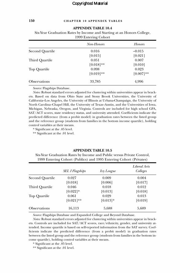
APPENDIX TABLE 10.4Six-Year Graduation Rates by Income and Starting at an Honors College,
1999 Entering Cohort
Non-Honors Honors
Second Quartile 0.016 –0.015[0.015] [0.021]
Third Quartile 0.051 0.007[0.018]** [0.010]
Top Quartile 0.098 0.023[0.019]** [0.007]**
Observations 33,785 4,996
Source: Flagships Database.Notes: Robust standard errors adjusted for clustering within universities appear in brack-
ets. Based on data from Ohio State and Stony Brook Universities, the University of California–Los Angeles, the University of Illinois at Urbana-Champaign, the University ofNorth Carolina–Chapel Hill, the University of Texas–Austin, and the Universities of Iowa,Michigan, Nebraska, Oregon, and Virginia. Controls are included for high school GPA,SAT/ACT scores, state residency status, and university attended. Coefficients indicate thepredicted difference (from a probit model) in graduation rates between the listed groupand the reference group (students from families in the bottom income quartile), holdingcontrol variables at their means.
* Significant at the .05 level.** Significant at the .01 level.
APPENDIX TABLE 10.5Six-Year Graduation Rates by Income and Public versus Private Control,
1999 Entering Cohort (Publics) and 1995 Entering Cohort (Privates)
Liberal Arts SEL I Flagships Ivy League Colleges
Second Quartile 0.027 0.009 0.004[0.018] [0.006] [0.017]
Third Quartile 0.046 0.018 0.012[0.022]* [0.013] [0.018]
Top Quartile 0.061 0.029 0.013[0.021]** [0.013]* [0.019]
Observations 16,113 5,688 5,609
Source: Flagships Database and Expanded College and Beyond Database.Notes: Robust standard errors adjusted for clustering within universities appear in brack-
ets. Controls are included for SAT/ACT scores, race/ethnicity, gender, and university at-tended. Income quartile is based on self-reported information from the SAT survey. Coef-ficients indicate the predicted difference (from a probit model) in graduation ratesbetween the listed group and the reference group (students from families in the bottom in-come quartile), holding control variables at their means.
* Significant at the .05 level.** Significant at the .01 level.
150 C H A P T E R 1 0 A P P E N D I X T A B L E S
Copyrighted MaterialCopyrighted MaterialCopyrighted Material
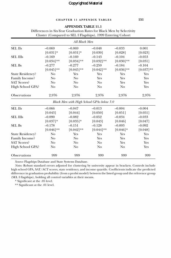
C H A P T E R 1 1 A P P E N D I X T A B L E S 151
APPENDIX TABLE 11.1Differences in Six-Year Graduation Rates for Black Men by Selectivity
Cluster (Compared to SEL I Flagships), 1999 Entering Cohort
All Black Men
SEL IIs –0.069 –0.069 –0.048 –0.033 0.001[0.031]* [0.031]* [0.030] [0.028] [0.023]
SEL IIIs –0.169 –0.169 –0.143 –0.104 –0.053[0.034]** [0.034]** [0.032]** [0.030]** [0.031]
SEL Bs –0.277 –0.277 –0.259 –0.184 –0.104[0.045]** [0.045]** [0.042]** [0.036]** [0.037]**
State Residency? No Yes Yes Yes YesFamily Income? No No Yes Yes YesSAT Scores? No No No Yes YesHigh School GPA? No No No No Yes
Observations 2,976 2,976 2,976 2,976 2,976
Black Men with High School GPAs below 3.0
SEL IIs –0.066 –0.047 –0.013 –0.004 –0.004[0.043] [0.044] [0.050] [0.051] [0.051]
SEL IIIs –0.090 –0.082 –0.052 –0.034 –0.033[0.037]* [0.035]* [0.043] [0.046] [0.047]
SEL Bs –0.178 –0.151 –0.128 –0.093 –0.092[0.046]** [0.042]** [0.044]** [0.046]* [0.048]
State Residency? No Yes Yes Yes YesFamily Income? No No Yes Yes YesSAT Scores? No No No Yes YesHigh School GPA? No No No No Yes
Observations 2,999 2,999 2,999 2,999 2,999
Source: Flagships Database and State Systems Database.Notes: Robust standard errors adjusted for clustering by university appear in brackets. Controls include
high school GPA, SAT/ACT scores, state residency, and income quartile. Coefficients indicate the predicteddifference in graduation probability (from a probit model) between the listed group and the reference group(SEL I flagships), holding all control variables at their means.
* Significant at the .05 level.** Significant at the .01 level.
Copyrighted MaterialCopyrighted MaterialCopyrighted Material

152 C H A P T E R 1 1 A P P E N D I X T A B L E S
APPENDIX TABLE 11.2Differences in Six-Year Graduation Rates for Hispanics by Selectivity
Cluster (Compared to SEL I Flagships), 1999 Entering Cohort
All Hispanics
SEL IIs –0.074 –0.075 –0.074 –0.078 –0.069 –0.052[0.030]* [0.030]* [0.029]* [0.027]** [0.026]** [0.025]*
SEL IIIs –0.194 –0.192 –0.191 –0.185 –0.158 –0.098[0.034]** [0.034]** [0.035]** [0.034]** [0.035]** [0.030]**
SEL Bs –0.324 –0.326 –0.333 –0.335 –0.284 –0.199[0.033]** [0.033]** [0.032]** [0.031]** [0.033]** [0.031]**
State Residency? No Yes Yes Yes Yes YesGender? No No Yes Yes Yes YesFamily Income? No No No Yes Yes YesSAT Scores? No No No No Yes YesHigh School GPA? No No No No No Yes
Observations 4,572 4,572 4,572 4,572 4,572 4,572
Hispanics with High School GPAs below 3.0
SEL IIs –0.105 –0.109 –0.096 –0.079 –0.071 –0.069[0.065] [0.069] [0.063] [0.066] [0.069] [0.081]
SEL IIIs –0.121 –0.121 –0.113 –0.094 –0.077 –0.064[0.071] [0.069] [0.066] [0.071] [0.078] [0.087]
SEL Bs –0.239 –0.244 –0.243 –0.231 –0.213 –0.162[0.071]** [0.073]** [0.067]** [0.070]** [0.081]** [0.092]
State Residency? No Yes Yes Yes Yes YesGender? No No Yes Yes Yes YesFamily Income? No No No Yes Yes YesSAT Scores? No No No No Yes YesHigh School GPA? No No No No No Yes
Observations 2,447 2,447 2,447 2,447 2,447 2,447
Source: Flagships Database and State Systems Database.Notes: Robust standard errors adjusted for clustering by university appear in brackets. Controls include
high school GPA, SAT/ACT scores, state residency, and income quartile. Coefficients indicate the predicteddifference in graduation probability (from a probit model) between the listed group and the reference group(SEL I flagships), holding all control variables at their means.
* Significant at the .05 level.** Significant at the .01 level.
Copyrighted MaterialCopyrighted MaterialCopyrighted Material