Chapter 1 Introduction - Princeton Universityassets.press.princeton.edu/chapters/s8535.pdf ·...

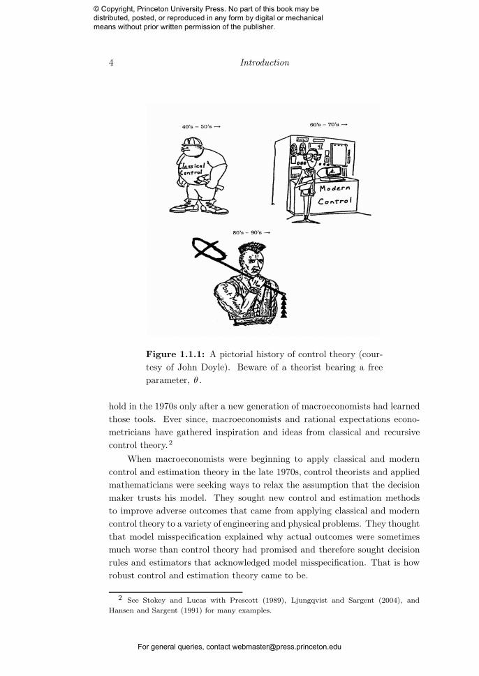
Chapter 1 Introduction

Knowledge would be fatal, it is the uncertainty that charms one. A mist makes things beautiful. — Oscar Wilde, The Picture of Dorian Gray, 1891

1.1. Generations of control theory

Figure 1.1.1 reproduces John Doyle’s cartoon about developments in optimal control theory since World War II.1 Two scientists in the upper panels use

different mathematical methods to devise control laws and estimators. The

person on the left uses classical methods (Euler equations, z -transforms, lag

operators) and the one on the right uses modern recursive methods (Bellman

equations, Kalman filters). The scientists in the top panels completely trust their models of the transition dynamics. The, shall we say, gentleman in the

lower panel shares the objectives of his predecessors from the 50s, 60s, and

70s, but regards his model as an approximation to an unknown and unspecified model that he thinks actually generates the data. He seeks decision

rules and estimators that work over a nondenumerable set of models near his approximating model. The H∞ in his postmodern tattoo and the θ on his

staff are alternative ways to express doubts about his approximating model by measuring the discrepancy of the true data generating mechanism from his approximating model. As we shall learn in later chapters, the parameter θ is interpretable as a penalty on a measure of discrepancy (entropy) between his approximating model and the model that actually generates the data. The

H∞ refers to the limit of his objective function as the penalty parameter θ approaches a “break down point” that bounds the set of alternative models against which the decision maker can attain a robust decision rule.

1.2. Control theory and rational expectations

Classical and modern control theory supplied perfect tools for applying Muth’s (1961) concept of rational expectations to a variety of problems in dynamic

economics. A significant reason that rational expectations initially diffused

slowly after Muth’s (1961) paper is that in 1961 few economists knew the

tools lampooned in the top panel of figure 1.1.1. Rational expectations took

1 John Doyle consented to let us reproduce this drawing, which appears in Zhou, Doyle, and Glover (1996). We changed Doyle’s notation by making θ (Doyle’s μ ) the free param

eter carried by the post-modern control theorist.

– 3 –

© Copyright, Princeton University Press. No part of this book may be distributed, posted, or reproduced in any form by digital or mechanical means without prior written permission of the publisher.

For general queries, contact [email protected]

4 Introduction

Figure 1.1.1: A pictorial history of control theory (courtesy of John Doyle). Beware of a theorist bearing a free

parameter, θ .

hold in the 1970s only after a new generation of macroeconomists had learned

those tools. Ever since, macroeconomists and rational expectations econometricians have gathered inspiration and ideas from classical and recursive

control theory.2

When macroeconomists were beginning to apply classical and modern

control and estimation theory in the late 1970s, control theorists and applied

mathematicians were seeking ways to relax the assumption that the decision

maker trusts his model. They sought new control and estimation methods to improve adverse outcomes that came from applying classical and modern

control theory to a variety of engineering and physical problems. They thought that model misspecification explained why actual outcomes were sometimes much worse than control theory had promised and therefore sought decision

rules and estimators that acknowledged model misspecification. That is how

robust control and estimation theory came to be.

2 See Stokey and Lucas with Prescott (1989), Ljungqvist and Sargent (2004), and Hansen and Sargent (1991) for many examples.



Misspecification and rational expectations 5

1.3. Misspecification and rational expectations

To say that model misspecification is as much of a problem in economics as it is in physics and engineering is an understatement. This book borrows, adapts, and extends tools from the literature on robust control and estimation to model decision makers who regard their models as approximations. We assume that a decision maker has created an approximating model by a

specification search that we do not model. The decision maker believes that data will come from3 an unknown member of a set of unspecified models near his approximating model.4 Concern about model misspecification induces a

decision maker to want decision rules that work over that set of nearby models.

If they lived inside rational expectations models, decision makers would

not have to worry about model misspecification. They should trust their model because subjective and objective probability distributions (i.e., models) coincide. Rational expectations theorizing removes agents’ personal models

as elements of the model.5

Although the artificial agents within a rational expectations model trust the model, a model’s author often doubts it, especially when calibrating it or after performing specification tests. There are several good reasons for

wanting to extend rational expectations models to acknowledge fear of model misspecification.6 First, doing so accepts Muth’s (1961) idea of putting econometricians and the agents being modeled on the same footing: because econometricians face specification doubts, the agents inside the model might too.7

Second, in various contexts, rational expectations models underpredict prices

3 Or, in the case of the robust filtering problems posed in chapter 17, have come from. 4 We say “unspecified” because of how these models are formed as statistical perturba

tions to the decision maker’s approximating model. 5 In a rational expectations model, each agent’s model (i.e., his subjective joint probabil

ity distribution over exogenous and endogenous variables) is determined by the equilibrium. It is not something to be specified by the model builder. Its early advocates in econometrics emphasized the empirical power that followed from the fact that the rational expectations hypothesis eliminates all free parameters associated with people’s beliefs. For example, see Hansen and Sargent (1980) and Sargent (1981).

6 In chapter 16, we explore several mappings, the fixed points of which restrict a robust decision maker’s approximating model. As is usually the case with rational expectations models, we are silent about the process by which an agent arrives at an approximating model. A qualification to the claim that rational expectations models do not describe the process by which agents form their models comes from the literature on adaptive learning. There, agents who use recursive least squares learning schemes eventually come to know enough to behave as they should in a self-confirming equilibrium. Early examples of such work are Bray (1982), Marcet and Sargent (1989), and Woodford (1990). See Evans and Honkapohja (2001) for new results.

7 This argument might offend someone with a preference against justifying modeling assumptions on behavioral grounds.



6 Introduction

of risk from asset market data. For example, relative to standard rational expectations models, actual asset markets seem to assign prices to macroeconomic risks that are too high. The equity premium puzzle is one manifestation

of this mispricing.8 Agents’ caution in responding to concerns about model misspecification can raise prices assigned to macroeconomic risks and lead to

reinterpreting them as compensation for bearing model uncertainty instead of risks with known probability distributions. This reason for studying robust decisions is positive and is to be judged by how it helps explain market data. A third reason for studying the robustness of decision rules to model misspecification is normative. A long tradition dating back to Friedman (1953), Bailey

(1971), Brainard (1967), and Sims (1971, 1972) advocates framing macroeconomic policy rules and interpreting econometric findings in light of doubts about model specification, though how those doubts have been formalized in

practice has varied.9

1.4. Our extensions of robust control theory

Among ways we adapt and extend robust control theory so that it can be

applied to economic problems, six important ones are discounting; a reinterpretation of the “worst-case shock process”; extensions to several multi-agent settings; stochastic interpretations of perturbations to models; a way of calibrating plausible fears of model misspecification as measured by the parameter θ in figure 1.1.1; and formulations of robust estimation and filtering problems.

1.4.1. Discounting

Most presentations of robustness in control theory treat undiscounted problems, and the few formulations of discounting that do appear differ from

the way economists would set things up.10 In this book, we formulate discounted problems that preserve the recursive structure of decision problems that macroeconomists and other applied economists use so widely.

8 A related finding is that rational expectations models impute low costs to business cycles. See Hansen, Sargent, and Tallarini (1999), Tallarini (2000), and Alvarez and Jer

mann (2004). Barillas, Hansen, and Sargent (2007) argue that Tallarini’s and Alvarez and Jermann’s measures of the costs of reducing aggregate fluctuations are flawed if what they measure as a market price of risk is instead interpreted as a market price of model uncertainty.

9 We suspect that his doubts about having a properly specified macroeconomic model explains why, when he formulated comprehensive proposals for the conduct of monetary and fiscal policy, Friedman (1953, 1959) did not use a formal Bayesian expected utility framework, like the one he had used in Friedman and Savage (1948).

10 Compare the formulations in Whittle (1990) and Hansen and Sargent (1995).



Our extensions of robust control theory 7

1.4.2. Representation of worst-case shock

As we shall see, in existing formulations of robust control theory, shocks that represent misspecification are allowed to feed back on endogenous state variables that are influenced by the decision maker, an outcome that in some

contexts appears to confront the decision maker with peculiar incentives to

manipulate future values of some of those shocks by adjusting his current decisions. Some economists11 have questioned the plausibility of the notion

that the decision maker is concerned about any misspecifications that can

be represented in terms of shocks that feed back on state variables under his partial control. In chapter 7, we use the “Big K , little k trick” from the

literature on recursive competitive equilibria to reformulate misspecification

perturbations to an approximating model as exogenous processes that cannot be influenced by the decision maker. As we illustrate in the analysis of the

permanent income model of chapter 10, this reinterpretation of the worst-case

shock process is useful in a variety of economic models.

1.4.3. Multiple agent settings

In formulations from the control theory literature, the decision maker’s model of the state transition dynamics is a primitive part of (i.e., an exogenous input into) the statement of the problem. In multi-agent dynamic economic problems, it is not. Instead, parts of the decision maker’s transition law governing

endogenous state variables, such as aggregate capital stocks, are affected by

other agents’ choices and therefore are equilibrium outcomes. In this book, we

describe ways of formulating the decision maker’s approximating model when

he and possibly other decision makers are concerned about model misspecification, perhaps to differing extents. We impose a common approximating model on all decision makers, but allow them to express different degrees of mistrust of that model and to have different objectives. As we explain in chapters 12, 15, and 16, this is a methodologically conservative approach that adapts the

concept of a Nash equilibrium to incorporate concerns about robustness. The

hypothesis of a common approximating model preserves much of the discipline of rational expectations, while the hypothesis that agents have different interests and different concerns about robustness implies a precise sense in

which ex post they behave as if they had different models. We thereby attain

a disciplined way of modeling apparent heterogeneity of beliefs.12

11 For example, Christopher Sims expressed this view to us. 12 Brock and deFontnouvelle (2000) describe a related approach to modeling heterogene

ity of beliefs.



8 Introduction

1.4.4. Explicitly stochastic interpretations

Much of this book is about linear-quadratic problems for which a convenient certainty equivalence result described in chapter 2 permits easy transitions between nonstochastic and stochastic versions of a problem. Chapter 3 describes the relationship between stochastic and nonstochastic setups.

1.4.5. Calibrating fear of misspecification

Rational expectations models presume that decision makers know the correct model, a probability distribution over sequences of outcomes. One way to justify this assumption is to appeal to adaptive theories of learning that endow

agents with very long histories of data and allow a Law of Large Numbers to

do its work.13 But after observing a short time series, a statistical learning

process will typically leave agents undecided among members of a set of models, perhaps indexed by parameters that the data have not yet pinned down

well. This observation is the starting point for the way that we use detection error probabilities to discipline the amount of model uncertainty that a

decision maker fears after having studied a data set of length T .

1.4.6. Robust filtering and estimation

Chapter 17 describes a formulation of some robust filtering problems that closely resemble problems in the robust control literature. This formulation

is interesting in its own right, both economically and mathematically. For one thing, it has the useful property of being the dual of a robust control problem. However, as we discuss in detail in chapter 17, this problem builds in a peculiar form of commitment to model distortions that had been chosen

earlier but that one may not want to consider when making current decisions. For that reason, in chapter 18, we describe a class of robust filtering and

estimation problems without commitment to those prior distortions. Here

the decision maker carries along the density of the hidden states given the

past signal history computed under the approximating model, then considers hypothetical changes in this density and in the state and signal dynamics

looking forward.

13 For example, see work summarized by Fudenberg and Levine (1998), Evans and Honkapohja (2001), and Sargent (1999a). The justification is incomplete because economies where agents use adaptive learning schemes typically converge to self-confirming equilibria, not necessarily to full rational expectations equilibria. They may fail to converge to rational expectations equilibria because histories can contain an insufficient number of observations about off-equilibrium-path events for a Law of Large Numbers to be capable of eradicating erroneous beliefs. See Cho and Sargent (2007) for a brief introduction to self-confirming equilibria and Sargent (1999a) for a macroeconomic application.



Entropy in specification analysis 9

1.5. Robust control theory, shock serial correlations, and rational expectations

Ordinary optimal control theory assumes that decision makers know a

transition law linking the motion of state variables to controls. The optimization problem associates a distinct decision rule with each specification

of shock processes. Many aspects of rational expectations models stem from

this association.14 For example, the Lucas critique (1976) is an application of the finding that, under rational expectations, decision rules are functionals of the serial correlations of shocks. Rational expectations econometrics achieves parameter identification by exploiting the structure of the function that maps shock serial correlation properties to decision rules.15

Robust control theory alters the mapping from shock temporal properties

to decision rules by treating the decision maker’s model as an approximation

and seeking a single rule to use for a set of vaguely specified alternative models expressed in terms of distortions to the shock processes in the approximating

model. Because they are allowed to feed back arbitrarily on the history of the

states, such distortions can represent misspecified dynamics. As emphasized by Hansen and Sargent (1980, 1981, 1991), the economet

ric content of the rational expectations hypothesis is a set of cross-equation

restrictions that cause decision rules to be functions of parameters that characterize the stochastic processes impinging on agents’ constraints. A concern

for model misspecification alters these cross-equation restrictions by inspiring the robust decision maker to act as if he had beliefs that seem to twist or slant probabilities in ways designed to make his decision rule less fragile

to misspecification. Formulas presented in chapters 2 and 7 imply that the

Hansen-Sargent (1980, 1981) formulas for those cross-equation restrictions

also describe the behavior of the robust decision maker, provided that we use

appropriately slanted laws of motion in the Hansen-Sargent (1980) forecasting

formulas. This finding shows how robust control theory adds a concern about misspecification in a way that preserves the econometric discipline imposed

by rational expectations econometrics.

1.6. Entropy in specification analysis

The statistical and econometric literatures on model misspecification supply

tools for measuring discrepancies between models and for thinking about decision making in the presence of model misspecification.

14 Stokey and Lucas with Prescott (1989) is a standard reference on using control theory to construct dynamic models in macroeconomics.

15 See Hansen and Sargent (1980, 1981, 1991).



∫

∫ ( )

∫

10 Introduction

Where y ∗ denotes next period’s state vector, let the data truly come

from a Markov process with one step transition density f(y ∗|y) that we assume has invariant distribution μ(y). Let the econometrician’s model be

fα(y ∗|y) where α ∈ A and A is a compact set of values for a parameter

vector α . If there is no α ∈ A such that fα = f , we say that the econometrician’s model is misspecified. Assume that the econometrician estimates α by maximum likelihood. Under some regularity conditions, the maximum

likelihood estimator α̂o converges in large samples to16

plim α̂o = argminα∈A I (fα, f) (y) dμ (y) (1.6.1)

where I(fα, f)(y) is the conditional relative entropy of model f with respect to model fα , defined as the expected value of the logarithm of the likelihood

ratio evaluated with respect to the true conditional density f(y ∗|y)

∗ I (fα, f) (y) = log f

f

α

((y

y

∗∗||y

y

))

f (y ∗ |y) dy . (1.6.2)

It can be shown that I(fα, f)(y) ≥ 0. Figure 1.6.1 depicts how the

probability limit α̂o of the estimator of the parameters of a misspecified model makes I(fα, f) = I(fα, f)(y)dμ(y) as small as possible. When the model is misspecified, the minimized value of I(fα, f) is positive.

A I(fαo , f)�

�

fαo

f

Figure 1.6.1: Econometric specification analysis. Suppose that the data generating mechanism is f and that the

econometrician fits a parametric class of models fα ∈ A to

the data and that f /∈ A . Maximum likelihood estimates of α eventually select the misspecified model fαo that is closest to f as measured by entropy I(fα, f).

Sims (1993) and Hansen and Sargent (1993) have used this framework to

deduce the consequences of various types of misspecification for estimates of

16 Versions of this result occur in White (1982, 1994), Vuong (1989), Sims (1993), Hansen and Sargent (1993), and Gelman, Carlin, Stern, and Rubin (1995).



∑

Acknowledging misspecification 11

parameters of dynamic stochastic models.17 For example, they studied the

consequences of using seasonally adjusted data to estimate models populated

by decision makers who actually base their decisions on seasonally unadjusted

data.

1.7. Acknowledging misspecification

To study decision making in the presence of model misspecification, we turn

the analysis of section 1.6 on its head by taking fαo as a given approximating model and surrounding it with a set of unknown possible data generating

processes, one unknown element of which is the true process f . See figure

1.7.1. Because he doesn’t know f , a decision maker bases his decisions on

the only explicitly specified model available, namely, the misspecified fαo . We are silent about the process through which the decision maker discovered

his approximating model fαo (y ∗|y).18 We also take for granted the decision

maker’s parameter estimates αo . 19 We impute some doubts about his model to the decision maker. In particular, the decision maker suspects that the

data are actually generated by another model f(y ∗|y) with relative entropy

I(fαo , f)(y). The decision maker thinks that his model is a good approximation in the sense that I(fαo , f)(y) is not too large, and wants to make

decisions that will be good when f � fαo . We endow the decision maker =

with a discount factor β and construct the following intertemporal measure

of model misspecification:20

∞I (fαo , f) = Ef βtI (fαo , f) (yt)

t=0

where Ef is the mathematical expectation evaluated with respect to the distribution f . Our decision maker confronts model misspecification by seeking a decision rule that will work well across a set of models for which

I(fαo , f) ≤ η0 , where η0 measures the set of models F surrounding his approximating model fα . Figure 1.7.1 portrays the decision maker’s view of the world. The decision maker wants a single decision rule that is reliable for

all models f in the set displayed in figure 1.7.1.21 This book describes how he

17 Also see Vuong (1989). 18 See Kreps (1988, chapter 11) for an interesting discussion of the problem of model

discovery. 19 In chapter 9, we entertain the hypothesis that the decision maker has estimated his

model by maximum likelihood using a data set of length T and use Bayesian detection error probabilities to guide the choice of a set of models against which he wants to be robust.

20 Hansen and Sargent (2005b, 2007a) provide an extensive discussion of reasons for adopting this measure of model misspecification.

21 ‘Reliable’ means good enough, but not necessary optimal, for each member of a set of



12 Introduction

can form such a robust decision rule by solving a Bellman equation that tells him how to maximize his intertemporal objective over decision rules when a

hypothetical malevolent nature minimizes that same objective by choosing a

model f . 22 That is, we use a max-min decision rule. Positing a malevolent nature is just a device that the decision maker uses to perform a systematic

analysis of the fragility of alternative decision rules and to construct a lower bound on the performance that can be attained by using them. A decision

maker who is concerned about robustness naturally seeks to construct bounds on the performance of potential decision rules, and the malevolent agent helps

the decision maker do that.

η

�

�

fαo

f

I(fαo , f) ≤ η

Figure 1.7.1: Robust decision making: A decision maker with model fαo suspects that the data are actually generated by a nearby model f , where I(fαo , f) ≤ η .

1.8. Why entropy?

To assess the robustness of a decision rule to misspecification of an approximating model requires a way to measure just how good an approximation

that model is. In this book, we use the relative entropy to measure discrepancies between models. Of course, relative entropy is not the only way we

models. The Lucas critique, or dynamic programming, tells us that it is impossible to find a single decision rule that is optimal for all f in this set. Note how the one-to-one mapping from transition laws f to decision rules that is emphasized in the Lucas critique depends on the decision maker knowing the model f . We shall provide a Bayesian interpretation of a robust decision rule by noting that, ex post , the max-min decision rule is optimal for some model within the set of models.

22 See Milnor (1951, 1954) for an early formal use of the fiction of a malevolent agent.



( ( ))

13 Why entropy?

could measure discrepancies between alternative probability distributions.23

But in using relative entropy, we follow a substantial body of work in applied

mathematics that reaps benefits from entropy in terms of tractability and

interpretability. In particular, using entropy to measure model discrepancies enables us to appeal to the following outcomes:

1. In the general nonlinear case, using entropy to measure model discrepancies means that concerns about model misspecification can be represented

in terms of a continuation value function that emerges as the indirect utility function after minimizing the decision maker’s continuation value with

respect to the transition density, subject to a penalty on the size of conditional entropy. That indirect utility function implies a tractable “risk-sensitivity” adjustment to continuation values in Bellman equations. In

particular, we can represent a concern about robustness by replacing

EtV (xt+1) in a Bellman equation with −θ log Et exp −V (θxt+1) , where

θ > θ > 0 is a parameter that measures the decision maker’s concern

about robustness to misspecification. (We shall relate the lower bound

θ to H∞ control theory in chapter 8.) The simple log Et exp form of this adjustment follows from the decision to measure model discrepancy

in terms of entropy.

2. In problems with quadratic objective functions and linear transition laws, using relative entropy to measure model misspecification leads to a simple adjustment to the ordinary linear-quadratic dynamic programming

problem. Suppose that the transition law for the state vector in the

approximating model is xt+1 = Axt + But + Cεt+1 , where εt+1 is an

i.i.d. Gaussian vector process with mean 0 and identity covariance. Using relative entropy to measure discrepancies in transition laws implies a worst-case model that perturbs the distribution of εt+1 by enhancing

its covariance matrix and appending a mean vector wt+1 that depends on date t information. Value functions remain quadratic and the distribution associated with the perturbed model remains normal. Because a

form of certainty equivalence prevails,24 it is sufficient to keep track of the mean distortion when solving the control problem. This mean distortion contributes .5wt+1 ·wt+1 to the relative entropy discrepancy between

the approximating model and the alternative model. As a consequence, a term θwt

′ +1wt+1 is appended to the one-period return function when

computing the robust control and a worst-case conditional mean.

23 Bergemann and Schlag (2005) use Prohorov distance rather than entropy to define the set of probability models against which decision makers seek robustness.

24 See page 33.



14 Introduction

3. As we shall see in chapter 9, entropy connects to a statistical theory for

discriminating one model from another. The theory of large deviations

mentioned in chapter 3 links statistical discrimination to a risk-sensitivity

adjustment.25

1.9. Why max-min?

We answer this question by posing three other questions.

1. What does it mean for a decision rule to be robust? A robust decision

rule performs well under the variety of probability models depicted in

figure 1.7.1. How might one go about investigating the implications of alternative models for payoffs under a given decision rule? A good way

to do this is to compute a lower bound on value functions by assessing

the worst performance of a given decision rule over a range of alternative

models. This makes max-min a useful tool for searching for a robust decision rule.

2. Instead of max-min, why not simply ask the decision maker to put a prior

distribution over the set of alternative models depicted in figure 1.7.1?

Such a prior would, in effect, have us form a new model – a so-called

hypermodel – and thereby eliminate concerns about the misspecification

of that model. Forming a hypermodel would allow the decision maker to

proceed with business as usual, albeit with what may be a more complex

model and a computationally more demanding control problem. We agree

that this “model averaging” approach is a good way to address some well-structured forms of model uncertainty. Indeed, in chapter 18 we shall use

model averaging and Bayesian updating when we study problems that call for combined estimation and control. But the set of alternative models can be so vast that it is beyond the capacity of a decision maker to conjure

up a unique well behaved prior. And even when he can, a decision maker might also want decisions to be robust to whatever prior he could imagine

over this set of models.

More is at issue than the choice of the prior distribution to assign to distinct well specified models. The specification errors that we fear might be more complex than can be represented with a simple model averaging approach. It is reasonable to take the view that each of the distinct models being averaged is itself an approximation. The decision maker might lack precise ideas about how to describe the alternative specifications that worry him and about how to form prior distributions over

25 Anderson, Hansen, and Sargent (2003) extensively exploit these connections.



Is max-min too cautious? 15

them. Perhaps he can’t articulate the misspecifications that he fears, or perhaps the set of alternative models is too big to comprehend.26

Our answer to this second question naturally leads to a reconsideration

of the standard justification for being a Bayesian.

3. “Why be a Bayesian?” Savage (1954) gave an authoritative answer by

describing axioms that imply that a rational person can express all of his

uncertainty in terms of a unique prior. However, Schmeidler (1989) and

Gilboa and Schmeidler (1989) altered one of Savage’s axioms to produce

a model of what it means to be a rational decision maker that differs

from Savage’s Bayesian model. Gilboa and Schmeidler’s rational decision

maker has multiple priors and behaves as a max-min expected utility

decision maker: the decision maker maximizes and assumes that nature

chooses a probability to minimize his expected utility. We are free to

appeal to Gilboa and Schmeidler’s axioms to rationalize the form of maxmin expected utility decision making embedded in the robust control theories that we study in this book.27

1.10. Is max-min too cautious?

Our doubts are traitors, And make us lose the good we oft might win, By

fearing to attempt. — William Shakespeare, Measure for Measure, act 1 scene 4

Our use of the detection error probabilities of chapter 9 to restrict the penalty

parameter θ in figure 1.1.1 protects us against the objection that the maxmin expected utility theory embedded in robust control theory is too cautious because, by acting as if he believed the worst-case model, the decision maker puts too much weight on a “very unlikely” scenario.28 We choose θ so that the entropy ball that surrounds the decision maker’s approximating model in

26 See Sims (1971) and Diaconis and Freedman (1986) for arguments that forming an appropriate prior is difficult when the space of submodels and the dimensions of parameter spaces are very large.

27 Hansen and Sargent (2001) and Hansen, Sargent, Turmuhambetova, and Williams (2006) describe how stochastic formulations of robust control “constraint problems” can be viewed in terms of Gilboa and Schmeidler’s max-min expected utility model. Interest

ing theoretical work on model ambiguity not explicitly connected to robust control theory includes Dow and Werlang (1994), Ghirardato and Marinacci (2002), Ghirardato, Mac

cheroni, and Marinacci (2004), Ghirardato, Maccheroni, Marinacci, and Siniscalchi (2003), and Rigotti and Shannon (2003, 2005), and Strzalecki (2007).

28 Bewley (1986, 1987, 1988), Dubra, Maccheroni, and Ok (2004), Rigotti and Shannon (2005), and Lopomo, Rigotti, and Shannon (2004) use an alternative to the max-min ex

pected utility model but still one in which the decision maker experiences ambiguity about models. In their settings, incomplete preferences are expressed in terms of model ambiguity



16 Introduction

figure 1.7.1 has the property that the perturbed models on and inside the ball are difficult to distinguish statistically from the approximating model with

the amount of data at hand. This way of calibrating θ makes the likelihood

function for the decision maker’s worst-case model fit the available data almost as well as his approximating model. Moreover, by inspecting the implied

worst-case model, we can evaluate whether the decision maker is focusing on

scenarios that appear to be too extreme.

1.11. Aren’t you just picking a plausible prior?

By interchanging the order in which we maximize and minimize, chapter 7 describes an ex post Bayesian interpretation of a robust decision rule.29 Friendly

critics have responded to this finding by recommending that we view robust control as simply a way to select a plausible prior in an otherwise standard

Bayesian analysis.30 Furthermore, one can regard our chapter 9 detection

error probability calculations as a way to guarantee that the prior is plausible

in light of the historical data record at the disposal of the decision maker. We have no objection to this argument in principle, but warn the reader

that issues closely related to the Lucas (1976) critique mean that it has to be

handled with care, as in any subjectivist approach. Imagine a policy intervention that alters a component of a decision maker’s approximating model for, e.g., a tax rate, while leaving other components unaltered. In general, all equations of the decision maker’s worst-case transition law that emerge

from the max-min decision process will vary with such interventions. The dependence of other parts of the decision maker’s worst-case model on subcomponents of the transition law for the approximating model that embody the

policy experiment reflects the context-specific nature of the decision maker’s

worst-case model. Therefore, parts of the ex post worst-case “prior” that describe the evolution of variables not directly affected by the policy experiment will depend on the policy experiment. The sense in which robust control is just a way to pick a plausible prior is subtle.

Another challenge related to the Lucas critique pertains when we apply

robust control without availing ourselves of the ex post Bayesian interpreta

and there is a status quo allocation that plays a special role in shaping how the decision maker ranks outcomes. Some advocates of this incomplete preferences approach say that they like it partly because it avoids what they say is an undue pessimism that characterizes the max-min expected utility model. See Fudenberg and Levine (1995) for how max-min can be used to attain an interesting convergence result for adaptive learning.

29 We introduce this argument because it provides a sense in which our robust decision rules are admissible in the statistical decision theoretic sense of being undominated.

30 Christopher A. Sims has made this argument on several occasions.



Why not learn the correct specification? 17

tion. Throughout this book, whenever we consider changes in the economic

environment, we imitate rational expectations policy analysis by imputing

common approximating models, one before the policy change, the other after, to all agents in the model and the econometrician (e.g., see chapter 14). It is natural to doubt whether decision makers would fully trust their statistical models after such policy changes.

1.12. Why not learn the correct specification?

For much of this book, but not all, we attribute an enduring fear of misspecification to our decision maker. Wouldn’t it be more realistic to assume that the

decision maker learns to detect and discard bad specifications as data accrue?

One good answer to this question is related to some of the points made

in section 1.9. In chapter 9, we suggest calibrating the free parameter θ borne by the “gentleman” in the bottom panel of figure 1.1.1 so that, even

with nondogmatic priors, it would take long time series to distinguish among

the alternative specifications about which the decision maker is concerned. Because our decision maker discounts the future, he cannot avoid facing up

to his model specification doubts simply by waiting for enough data.31 Thus, one answer is that, relative to his discount factor, it would take a long time

for him to learn not to fear model misspecification. However, we agree that it is wise to think hard about what types of

misspecification fears you can expect learning to dispel in a timely way, and

which types you cannot. But what are good ways to learn when you distrust your model? Chapters 17 and 18 are devoted to these issues.32 We present alternative formulations of robust estimation and filtering problems and suggest ways to learn in the context of distrusted approximating models. Our approach allows us to distinguish types of model misspecification fears that a decision maker can eventually escape by learning from types that he

cannot.33

31 As we shall see, one reason that it takes a very long data set to discriminate between the models that concern the decision maker is that often they closely approximate each other at high frequencies and differ mostly at very low frequencies. Chapter 8 studies robustness from the viewpoint of the frequency domain.

32 Also see Hansen and Sargent (2005b, 2007a, 2007b). 33 Epstein and Schneider (2006) also make this distinction. In the empirical model of

Hansen and Sargent (2007b), a representative consumer’s learning within the sample period reduces his doubts about the distribution of some unknown parameters, but does little to diminish his doubts about the distribution over difficult to distinguish submodels, one of which confronts him with long-run risk in the growth rate of consumption.



18 Introduction

1.13. Is the set of perturbed models too limited?

Parts of this book are devoted to analyzing situations in which the decision maker’s approximating model and the statistical perturbations to it that bother him all take the form of the stochastic linear evolution

xt+1 = Axt + But + C (εt+1 + wt+1) (1.13.1)

where xt is a state vector, ut a control vector, εt+1 an i.i.d. Gaussian shock

with mean 0 and covariance I , and wt+1 is a vector of perturbations to the

mean of εt+1 . Under the approximating model, wt+1 = 0, whereas under perturbed models, wt+1 is allowed to be nonzero and to feed back on the

history of past xt ’s. Some critics have voiced the complaint that this class of perturbations ex

cludes types of misspecified dynamics that ought to concern a decision maker, such as unknown parameter values, misspecfication of higher moments of the

εt+1 distribution, and various kinds of “structured uncertainty.” We think

that this complaint is misplaced for the following reasons:

1. For the problems with quadratic objective functions and approximating

models like (1.13.1) with wt+1 = 0, restricting ourselves to perturbations of the form (1.13.1) turns out not to be as restrictive as it might at first seem. In chapters 3 and 7, we permit a much wider class of alternative

models that we formulate as absolutely continuous perturbations to the

transition density of state variables. We show that when the decision

maker’s objective function is quadratic and his approximating model is linear with Gaussian εt+1 , then he chooses a worst-case model that is of the form (1.13.1) with a C that is usually only slightly larger and a wt+1

that is a linear function of xt . We shall explain why he makes little or no error by ignoring possible misspecification of the volatility matrix C .

2. In section 19.2 of chapter 19, we show how more structured kinds of uncertainty can be accommodated by slightly reinterpreting the decision

maker’s objective function.

3. When the approximating model is a linear state evolution equation with

Gaussian disturbances and the objective function is quadratic, worst case

distributions are also jointly Gaussian. However, making the approximating model be non-Gaussian and non-linear or making the objective function be not quadratic leads to non-Gaussian worst-case joint probability

distributions, as chapter 3 indicates. Fortunately, by extending the methods of chapters 17 and 18, as Hansen and Sargent (2005, 2007a) do, we

know how to model robust decision makers who learn about non-linear



Other lessons 19

models with non-Gaussian shock distributions while making decisions. The biggest hurdles in carrying out quantitative analyses like these are

computational. Most of the problems studied in this book are designed

to be easy computationally by staying within a linear-quadratic-Gaussian

setting. But numerical methods allow us to tackle analogous problems

outside the LQG setting.34

1.14. Is robust control theory positive or normative?

Robust control and estimation theory has both normative and positive economic applications. In some contexts, we take our answer to question (2) in

the preceding section to justify a positive statement about how people actually

behave. For example, we use this interpretation when we apply robust control and estimation theory to study asset pricing puzzles by constructing a robust representative consumer whose marginal evaluations determine market prices of risk (see Hansen, Sargent, and Tallarini (1999), Hansen, Sargent, and Wang

(2002), and chapter 13). Monetary policy authorities and other decision makers find themselves

in situations where their desire to be cautious with respect to fears of model misspecification would inspire them to use robust control and estimation techniques.35 Normative uses of robust control theory occur often in engineering.

1.15. Other lessons

Our research program of refining typical rational expectations models to attribute specification doubts to the agents inside of them has broadened our own understanding of rational expectations models themselves. Struggling

with the ideas in this book has taught us much about the structure of recursive models of economic equilibria,36 the relationship between control and

estimation problems, and Bayesian interpretations of decision rules in dynamic rational expectations models. We shall use the macroeconomist’s Big

K , little k trick with a vengeance. The 1950s-1960s control and estimation theories lampooned in the top

panel of figure 1.1.1 have contributed enormously to the task of constructing

dynamic equilibrium models in macroeconomics and other areas of applied

economic dynamics. We expect that the robust control theories represented

34 See Cogley, Colacito, Hansen, and Sargent (2007) for an example. 35 Blinder (1998) expresses doubts about model misspecification that he had when he

was vice chairman of the Federal Reserve System and how he coped with them. 36 For example, see chapter 12.



20 Introduction

in the bottom panel of that figure will also bring many benefits that we cannot anticipate.

1.16. Topics and organization

This monograph displays alternative ways to express and respond to a decision maker’s doubts about model specification. We study both control and

estimation (or filtering) problems, and both single- and multiple-agent settings. As already mentioned, we adapt and extend results from the robust control literature in two important ways. First, unlike the control literature, which focuses on undiscounted problems, we formulate discounted problems. Incorporating discounting involves substantial work, especially in chapter 8, and requires paying special attention to initial conditions. Second, we analyze

three types of economic environments with multiple decision makers who are

concerned about model misspecification: (1) a competitive equilibrium with

complete markets in history-date contingent claims and a representative agent who fears model misspecification (chapters 12 and 13); (2) a Markov perfect equilibrium of a dynamic game with multiple decision makers who fear model misspecification (chapter 15); and (3) a Stackelberg or Ramsey problem in

which the leader fears model misspecification (chapter 16). Thinking about model misspecification in these environments requires that we introduce an

equilibrium concept that extends rational expectations. We stay mostly, but not exclusively, within a linear-quadratic framework, in which a pervasive certainty equivalence principle allows a nonstochastic presentation of most of the

control and filtering theory.

This book is organized as follows. Chapter 2 summarizes a set of practical results at a relatively nontechnical level. A message of this chapter

is that although sophisticated arguments from chapters 7 and 8 are needed

fully to justify the techniques of robust control, the techniques themselves are as easy to apply as the ordinary dynamic programming techniques that are now widely used throughout macroeconomics and applied general equilibrium theory. Chapter 2 uses linear-quadratic dynamic problems to convey

this message, but the message applies more generally, as we shall illustrate in

chapter 3. Chapter 3 tells how the key ideas about robustness generalize to

models that are not linear quadratic.

Chapters 4 and 5 are about optimal control and filtering when the decision maker trusts his model. These chapters contain a variety of useful results for characterizing the linear dynamic systems that are widely used in macroeconomics. Chapter 4 sets forth important principles by summarizing results about the classic optimal linear regulator problem. This chapter builds on



21 Topics and organization

the survey by Anderson, Hansen, McGrattan, and Sargent (1996) and culminates in a description of invariant subspace methods for solving linear optimal control and filtering problems and also for solving dynamic linear equilibrium

models. Later chapters apply these methods to various problems: to compute

robust decision rules as solutions of two-player zero-sum games; to compute

robust filters via another two-player zero-sum game; and to compute equilibria of robust Stackelberg or Ramsey problems in macroeconomics. Chapter 5

emphasizes that the Kalman filter is the dual (in a sense familiar to economists from their use of Lagrange multipliers) of the basic linear-quadratic dynamic

programming problem of chapter 4 and sets the stage for a related duality

result for a robust filtering problem to be presented in chapter 17.

The remaining chapters are about making wise decisions when a decision

maker distrusts his model. Within a one-period setting, chapter 6 introduces two-player zero-sum games as a way to induce robust decisions. Although

the forms of model misspecifications considered in this chapter are very simple relative to those considered in subsequent chapters, the static setting of chapter 6 is a good one for addressing some important conceptual issues. In

particular, in this chapter we state multiplier and constraint problems, two

different two-player zero-sum games that induce robust decision rules. We use

the Lagrange multiplier theorem to connect the problems.

Chapters 7 and 8 extend and modify results in the control literature to formulate robust control problems with discounted quadratic objective functions

and linear transition laws. Chapter 7 represents things in the time domain, while chapter 8 works in the frequency domain. Incorporating discounting

requires carefully restating the control problems used to induce robust decision rules. Chapters 7 and 8 describe two ways to alter the discounted linear

quadratic optimal control problem in a way to induce robust decision rules: (1) to form one of several two-player zero-sum games in which nature chooses

from a set of models in a way that makes the decision maker want robust decision rules; and (2) to adjust the continuation value function in the dynamic

program in a way that encodes the decision maker’s preference for a robust rule. The continuation value that works comes from the minimization piece

of one of the two-player zero-sum games in (1). In category (1), we present a detailed account of several two-player zero-sum games with different timing

protocols, each of which induces a robust decision rule. As an extension of category (2), we present three specifications of preferences that express concerns

about model misspecification. Two of them are expressed in the frequency

domain: the H∞ and entropy criteria. The entropy objective function summarizes model specification doubts with a single parameter. That parameter relates to a Lagrange multiplier in a two-player zero-sum constraint game, and



22 Introduction

also to the risk-sensitivity parameter of Jacobson (1973) and Whittle (1990), as modified for discounting by Hansen and Sargent (1995).

Chapters 7 and 8 show how robustness is induced by using max-min

strategies: the decision maker maximizes while nature minimizes over a set of models that are close to the approximating model. There are alternative

timing protocols in terms of which a two-player zero-sum game can be cast. A main finding of chapter 7 is that zero-sum games that make a variety of different timing protocols share outcomes and representations of equilibrium

strategies. This important result lets us use recursive methods to compute

our robust rules and also facilitates computing equilibria in multiple-agent economics.

Arthur Goldberger and Robert E. Lucas, Jr., warned applied economists to beware of theorists bearing free parameters (see figure 1.1.1). Relative to

settings in which decision makers completely trust their models, the multiplier and constraint problems of chapters 7 and 8 each bring one new free parameter that expresses a concern about model misspecification, θ for the multiplier problem and η for the constraint problem. Each of these parameters measures

sets of models near the approximating model against which the decision maker

seeks a robust rule. Chapter 9 proposes a way to calibrate these parameters

by using the statistical theory for discriminating models.37 We apply this theory in chapters 10 and 14.

Chapter 10 uses the permanent income model of consumption as a laboratory for illustrating some of the concepts from chapters 7 and 8. Because he

prefers smooth consumption paths, the permanent income consumer’s savings are designed to attenuate the effects of income fluctuations on his consumption. A robust consumer engages in a kind of precautionary savings because

he suspects error in the specification of the income process. We will also use

the model of chapter 10 as a laboratory for asset pricing in chapter 13. But first, chapters 11 and 12 describe how to decentralize the solution of a planning problem with a competitive equilibrium. Chapter 11 sets out a class of dynamic economies and describes two decentralizations, one with trading of history-date contingent commodities once and for all at time zero, another

with sequential trading of one-period Arrow securities. In that sequential setting, we give a recursive representation of equilibrium prices. Chapter 11

describes a setting where the representative agent has no concern about model misspecification, while chapter 12 extends the characterizations of chapter 11

to situations where the representative decision maker fears model misspecification.

Chapter 13 builds on the chapter 12 results to show how fear of model

37 See Anderson, Hansen, and Sargent (2003).



Topics and organization 23

misspecification affects asset pricing. We show how, from the vantage point of the approximating model, a concern for robustness induces a multiplicative

adjustment to the stochastic discount factor. The adjustment measures the

representative consumer’s fear that the approximating model is misspecified. The adjustment for robustness resembles ones that financial economists use

to construct risk neutral probability measures for pricing assets. We describe

the basic theory within a class of linear quadratic general equilibrium models and then a calibrated version of the permanent income model of chapter 10. A remarkable observational equivalence result identifies a locus of pairs of discount factors and robustness multipliers, all of which imply identical real allocations.38 Nevertheless, prices of risky assets vary substantially across

these pairs. In chapter 14, we revisit some quantitative findings of Tallarini (2000) and reinterpret asset pricing patterns that he imputed to very high risk

aversion in terms of a plausible fear of model misspecification. We measure

a plausible fear of misspecification by using the detection error probabilities introduced in chapter 9.

Chapters 15 and 16 describe two more settings with multiple decision

makers and introduce an equilibrium concept that extends rational expectations in what we think is a natural way. In a rational expectations equilibrium, all decision makers completely trust a common model. Important aspects of that common model, those governing endogenous state variables, are equilibrium outcomes. The source of the powerful cross-equation restrictions that are the hallmark of rational expectations econometrics is that decision makers share a common model and that this model governs the data.39 To preserve

that empirical power in an equilibrium with multiple decision makers who fear model misspecification, we impose that all decision makers share a common

approximating model.40 The model components that describe endogenous state variables are equilibrium outcomes that depend on agents’ robust decision making processes, i.e., on the solutions to their max-min problems.

Chapter 15 describes how to implement this equilibrium concept in the

context of a two-player dynamic game in which the players share a common

38 This result establishes a precise sense in which, so far as real quantities are concerned, increased fear of model misspecficiation acts just like reduced discounting of the future, so that its effects on real quantities can be offset by increasing the rate at which future payoffs are discounted.

39 The restriction that they share a common model is the feature that makes free pa

rameters governing expectations disappear. This is what legitimizes a law of large numbers that underlies rational expectations econometrics.

40 In the empirical applications of Hansen, Sargent, and Tallarini (1999) and Anderson, Hansen, and Sargent (2003), we also maintain the second aspect of rational expectations modeling, namely, that the decision makers’ approximating model actually does generate the data.



24 Introduction

approximating model and each player makes robust decisions by solving a two-player zero-sum game, taking the approximating model as given. We show

how to compute the approximating model by solving pairs of robust versions of the Bellman equations and first-order conditions for the two decision makers. While the equilibrium imposes a common approximating model, the worst-case models of the two decision makers differ because their objectives differ. In this sense, the model produces endogenous ex post heterogeneity of beliefs.

In chapter 16, we alter the timing protocol to study a control problem, called a Ramsey problem, where a leader wants optimally to control followers who are forecasting the leader’s controls. We describe how to compute a

robust Stackelberg policy when the Stackelberg leader can commit to a rule. We accomplish that by using a robust version of the optimal linear regulator

or else one of the invariant subspace methods of chapter 4. Chapter 17 extends the analysis of filtering from chapter 5 by describing

a robust filtering problem that is dual to the control problem of chapter 7.41

This recursive filtering problem requires that a time t decision maker must respect distortions to the distribution of the hidden state that he inherits from past decision makers. As a consequence, in this problem, bygones are

not bygones:42 the decision makers concerns about past returns affect his

estimate of the current value of a hidden state vector. Chapter 18 uses a different criterion than chapter 17 and finds a different

robust filter. We think that the chapter 18 filter is the appropriate one for many problems and give some examples. The different filters that emerge from

chapters 17 and 18 illustrate how robust decision rules are ‘context specific’ in the sense that they depend on the common objective function in the two-player zero-sum game that is used to induce a robust decision rule. This theme will run through this book.

Chapter 19 concludes by confronting some of the confining aspects of our work, some criticisms that we have heard, and opportunities for further progress.

41 We originally found this problem by stating and solving a conjugate problem of a kind familiar to economists through duality theory. By faithfully following where duality leads, we discovered a filtering problem that is peculiar (but not necessarily uninteresting) from an economic standpoint. A sketch of this argument is presented in appendix A of chapter 17.

42 But see the epigraph from William Stanley Jevons quoted at the start of chapter 18.



Chapter 1 Introduction - Princeton Universityassets.press.princeton.edu/chapters/s8535.pdf ·...

Documents

Transcript of Chapter 1 Introduction - Princeton Universityassets.press.princeton.edu/chapters/s8535.pdf ·...