Cross-ownership, R&D Spillovers, and Antitrust...

Cross-ownership, R&D Spillovers, and Antitrust

Policy�

Ángel L. Lópezy Xavier Vivesz

May 2016

Abstract

This paper considers cost-reducing R&D investment with spillovers in a Cournot

oligopoly with minority shareholdings. We �nd that, with high market concen-

tration and su¢ ciently convex demand, there is no scope for cross-ownership to

improve welfare regardless of spillover levels. Otherwise, there is scope for cross-

ownership provided that spillovers are su¢ ciently large. The socially optimal degree

of cross-ownership increases with the number of �rms, with the elasticity of demand

and of the innovation function, and with the extent of spillover e¤ects. In terms of

consumer surplus standard, the scope for cross-ownership is greatly reduced even

under low market concentration.

JEL classi�cation numbers: D43, L13, O32Keywords: competition policy; partial merger; collusion; innovation; minority sharehold-ings; modi�ed HHI

�We thank Ramon Faulí-Oller for his insightful initial contributions to this paper. For helpful com-ments we thank Isabel Busom, Luis Cabral, Guillermo Caruana, Ricardo Flores-Fillol, Richard Gilbert,Gerard Llobet, Peter Neary, Patrick Rey, Yossi Spiegel, and Javier Suarez. We have received constructivesuggestions from seminar participants at IESE (PPSRC), Universität Mannheim, Università di Bologna,Universitat de Barcelona, CEMFI, Paris School of Economics, and Universitat Rovira i Virgili as well asfrom conference participants at CRESSE 2012, �Industrial Organization and Spatial Economics�(HSE,Saint Petersburg), 5th Barcelona IO Workshop (Universitat Pompeu Fabra), EEA2013 (University ofGothenburg), Barcelona GSE Winter Workshop 2013 (IAE-CSIC), CEPR Applied IO Workshop 2014,Searle Antitrust Conference 2014, EARIE 2014, XXIX Jornadas de Economía Industrial (BarcelonaGSE), the ES Boston Meeting 2015, the Barcelona GSE Summer Forum 2015, the World Congress of theEconometric Society 2015, and SAEe 2015. Financial support from the Spanish Ministry of Science andInnovation under ECO2011-29533, from the Spanish Ministry of Economy and Competitiveness underECO2015-63711-P, and from AGAUR under SGR 1326 (GRC), is gratefully acknowledged.

yLópez: Departament d�Economia Aplicada, Universitat Autònoma de Barcelona, and Public-PrivateSector Research Center, IESE Business School. E-mail address: [email protected]

zVives: IESE Business School.

1

1 Introduction

In many industries, minority shareholdings are prevalent in the form of cross-shareholding

agreements among �rms or common ownership by investment funds. The tendency of such

arrangements to reduce price competition has been documented in the airline and banking

industries (Azar et al. 2015, 2016), and it has raised antitrust concerns. However, cross-

ownership arrangements (COAs) may have a bene�cial e¤ect on investment provided

there are positive spillovers across �rms. The reason is that COAs help to internalize the

spillover externality, which is especially important for highly innovative industries. To

what extent, and by what means, should antitrust authorities limit the �partial�mergers

that result from cross-ownership in innovative industries? In this paper we provide a wel-

fare analysis of COAs� when �rms compete in quantities and invest in cost reduction� in

the presence of spillovers; we also derive some implications for competition policy. The

analysis may help elucidate whether the documented increase in cross-ownership arrange-

ments has outrun its social value.

We consider a general symmetric model of cross-ownership; this model allows for

a range of corporate control and for distinguishing between stock acquisitions made by

investors and those made by other �rms. In our benchmark model, we consider simultane-

ous R&D and output decisions. That approach aids tractability while helping to capture

the imperfect observability of �rms�R&D investment levels.1 We test the robustness of

results by way of a two-stage speci�cation. The model subsumes earlier contributions to

the literature that were based on linear or constant elasticity of demand and on spe-

ci�c innovation functions (Dasgupta and Stiglitz 1980; Spence 1984; d�Aspremont and

Jacquemin 1988; Kamien et al. 1992). Perhaps the work closest to ours in spirit is the

paper by Leahy and Neary (1997).

Our paper seeks to answer the following questions: How do R&D and output levels

vary with minority shareholdings? What are the key determinants of the socially optimal

extent of cross-ownership? How is that optimal level a¤ected by structural parameters

(demand and cost conditions, industry technological opportunity, extent of spillovers) and

by the competition authority�s objective (to maximize total or rather consumer surplus)?

The main results can be summarized as follows. If demand is not too convex, then

1Simultaneous models� in the presence or absence of R&D spillovers� are analyzed by, among others,Dasgupta and Stiglitz (1980), Hartwick (1984), Levin and Reiss (1988), Ziss (1994), Leahy and Neary(1997), Cabral (2000), and Vives (2008).

2

increasing the partial ownership interest in rivals will increase (resp. decrease) both R&D

and output when spillovers are high (resp. low); for intermediate levels of spillovers,

an increase in such ownership interest will increase R&D but reduce output. These are

testable predictions. We identify the key determinants of a welfare-optimal degree of

cross-ownership: the curvature of demand, the degree of market concentration, and the

extent of spillovers. A su¢ cient (but not necessary) condition for the absence of minority

shareholdings to be optimal� from either the total surplus (TS) or consumer surplus (CS)

perspective, and for any extent of spillover� is that the relative degree of convexity of

demand be greater than the inverse of the Her�ndahl�Hirschman index (HHI). Otherwise,

the range of spillovers is typically partitioned into three regions: one optimally with no

cross-ownership for low levels of spillovers; one optimally with positive cross-ownership

(by TS and CS standards) for high levels of spillovers; and one optimally with positive

cross-ownership (by the TS standard only) in an intermediate region. We remark that the

consumer surplus standard is always more stringent than the total surplus standard. We

also �nd that, if the e¤ectiveness of R&D is independent of the degree of cross-ownership,

then under the CS standard there is a �bang bang� solution: either independent own-

ership or cartelization is optimal. Numerical results reveal that the (TS-based) socially

optimal extent of cross-ownership is increasing in the number of �rms, in the elasticity of

demand and of the innovation function, and in the level of spillover e¤ects. Qualitatively

similar results hold for the CS-based optimal extent, except that the scope for minority

shareholdings is much reduced.

The context analyzed here is of more than theoretical interest. Minority sharehold-

ings are widespread in many industries (e.g., automobiles, airlines, �nancial, energy, and

steel) and have attracted increasing antitrust attention (see EC 2013). There is grow-

ing interest among competition authorities in assessing the competitive e¤ects of partial

stock acquisitions. This increased attention stems mainly from two factors: (i) the rapid

growth of private equity investment �rms, which often hold partial ownership interests

in competing �rms (Wilkinson and White 2007); and (ii) some notorious cases, such as

Ryanair�s acquisition of Aer Lingus�s stock and the Renault�Nissan alliance (under which

Renault owns 44.3% of Nissan even as Nissan owns 15% of Renault).2 These factors have

2As Gino (2000) delineates, four other cases that have attracted considerable interest are as follows:(i) a $150 million investment by Microsoft in the nonvoting stock of Apple in 1997; (ii) the purchase byNorthwest Airlines (fourth-largest US airline) of 14% of the common stock of Continental Airlines (the

3

triggered a debate in Europe over the possibly anticompetitive e¤ects of partial owner-

ship. Yet the European Commission (EC) is not authorized to examine the acquisition of

minority shareholdings,3 and it has proposed extending the scope of its merger regulations

so that it can intervene in cases involving minority shareholdings among competitors or

in a vertical relationship (EC 2014).4 In Canada and the United States, cross-ownership

is scrutinized under prevailing merger control rules. More speci�cally, minority share-

holdings in the latter country are often examined with reference to the Clayton Act and

the Hart�Scott�Rodino Act.5 However, there is an exception to antitrust scrutiny if the

participation is �solely for investment� purposes, although it is subject to interpreta-

tion whether institutional investors can hold as much as 15% without needing to notify.

These US provisions are important because common ownership by investment funds is

widespread in many sectors.6

The extant literature, most of which focuses on the potential bene�ts of cooperative

R&D or on how innovation is a¤ected by mergers, has largely ignored the topic of how

innovation is a¤ected by minority shareholdings� despite clear evidence that antitrust

policy attends closely to innovation. During the period 2008�2014, 36% of the mergers

challenged by the US Department of Justice or the US Federal Trade Commission were

characterized as harmful to innovation; of the challenged mergers, 76% were in high�

R&D intensity industries. The anticompetitive e¤ects of minority shareholdings tend to

be weaker than those of a merger; at the same time, minority shareholdings seldom

yield the e¢ ciencies (e.g., rationalization, fewer duplicated costs) that may arise from a

�fth-largest) while agreeing to limit its voting power (however, an antitrust suit forced Northwest to sellback nearly half of its purchased stake); (iii) the purchase by TCI (largest US cable operator) of a 9%stake in Time Warner (the second-largest); (iv) the acquisition by Gillette of more than a �fth of thenonvoting stock (and more than a tenth of the debt) of Wilkinson Sword, one of its main competitors.

3In some European countries (e.g., Austria, Germany, the United Kingdom), national merger controlrules give competition authorities the scope to examine minority shareholdings. Currently, the EC canconsider the e¤ects on competition only of (pre-existing) minority shareholdings in the context of ananticipatedOK? merger (and in which the merging �rms each have stakes in a third �rm).

4The European Commission (EC 2014) has proposed a �targeted transparency�system under whichthe EC and its member states must be noti�ed of potentially harmful acquisitions. Included in this cat-egory would be acquisitions of a minority shareholding� in a competitor or vertically related company�when either the acquired shareholding amounts to 20% or ranges between 5% and 20% but allows theacquirer �a de-facto blocking minority, a seat on the board of directors, or access to commercially sensitiveinformation of the target" (p. 13).

5Section 7 of the Clayton Act prohibits acquisitions (of any part) of a company�s stock that �may�substantially lessen competition either by (a) enabling the acquirer to manipulate, directly or indirectly,prices or output or by (b) reducing its own incentives to compete. Although there is no clearly establishedthreshold, acquisitions of less than 25%� but of at least 15%� have been adjudged to be in violation(Salop and O�Brien 2000).

6See Azar et al. (2015, 2016).

4

merger. The commonly held view is that, overall, minority shareholdings tend to lessen

competition. Nonetheless, the evidence of spillover-induced underinvestment in R&D

suggests that cross-ownership could be bene�cial.7

The paper proceeds as follows. We review the literature in Section 2. In Section 3, we

describe the di¤erent types of minority shareholdings that can be analyzed via our model,

which is presented in Section 4. That section characterizes the equilibrium responses of

output and R&D in response to a change in the degree of cross-ownership. In Section 5, we

examine the socially optimal degree of cross-ownership and then illustrate the results with

three leading speci�cations from the literature: the d�Aspremont�Jacquemin and Kamien�

Muller�Zang models, and a constant elasticity model as in Dasgupta and Stiglitz (1980).

Section 6 extends our model to allow for strategic R&D commitments in a two-stage

game. Section 7 explores an alternative interpretation of our model when cooperation in

R&D extends to the product market; with regard to this case there is empirical evidence,

antitrust case study evidence, and also experimental evidence. We conclude in Section 8.

Unless noted otherwise, all proofs are given in Appendix A. Appendix B provides details

on our analysis of the three model speci�cations considered. Note that we o¤er application

software (available on the Web), which the reader can use to conduct simulations with

the models.

2 Review of the literature

Previous literature has analyzed the anticompetitive e¤ects of cross-ownership (Bresna-

han and Salop 1986; Reynolds and Snapp 1986). These researchers show that the pres-

ence of partial ownership interests in a Cournot industry may result in less output and

higher prices (even if those interests are relatively small). This is because the compet-

itive decisions of one �rm� with stakes in a competitor�s pro�t� will take those stakes

into account by reducing output (or raising the price) so as to increase that competitor�s

pro�t and hence its own �nancial pro�t. Azar et al. (2015) document the substantial

common ownership interests of institutional investors (e.g., BlackRock, Vanguard, State

Street, Fidelity) in competing technology �rms (Apple, Microsoft), pharmacies (CVS,

7For example, Bloom et al. (2013) report underinvestment in R&D (because of spillovers) in a panelof US �rms from 1981 to 2001. These authors �nd that (i) the e¤ects of technology spillovers are muchgreater than those of product market spillovers and (ii) the socially optimal level of R&D is 2�3 timesas high as the observed level of R&D.

5

Walgreens), and banks (JP Morgan Chase, Bank of America, Citigroup). In that study

of how passive investments by institutional investors a¤ect market outcomes in the US

airline industry, the authors �nd that ticket prices are about 10% higher on the average

route than they would be with no cross-ownership (or if strategy decisions were made

without regard to the investors�minority shareholdings). Similar results are obtained for

the banking industry (Azar et al. 2016).

There is an extensive literature on the e¤ects of cooperation and competition in R&D

with spillovers, starting from the seminal articles of Brander and Spencer (1984), Spence

(1984), Katz (1986), and d�Aspremont and Jacquemin (1988, 1990). Leahy and Neary

(1997) present a general analysis of the e¤ects of strategic behavior and cooperative R&D

in the presence of price and output competition; they also study optimal public policy

toward R&D in the form of subsidies.8 One of this literature�s primary objectives is to

examine underprovision of R&D and the welfare e¤ects of moving from a noncooperative

to a cooperative regime in R&D. For example, d�Aspremont and Jacquemin (1988, 1990)

show that, when spillovers are high enough, R&D cooperation (with subsequent competi-

tion at the output stage) leads to increased output, innovation, and welfare. Cooperative

R&D enables �rms to internalize their externalities and thus preserves the incentives to

invest in R&D.

We shall identify the conditions under which minority shareholdings may increase total

surplus, and even consumer surplus, in industries where R&D investment is important

and spillovers are signi�cant. Farrell and Shapiro (1990) show that passive �nancial

stakes may be welfare increasing in asymmetric oligopolies; here we demonstrate the

possibility in a symmetric oligopoly. There is some evidence that common ownership

improves e¢ ciency. He and Huang (2014), using data on US public �rms from 1980 to

2010, estimate the e¤ect of common ownership on market performance and report that

�rms increase their market share (up to 3.2%) through common ownership.9

The results that we derive complement those in the extant literature. For instance,

Leahy and Neary (1997) �nd that R&D cooperation leads both to more output and

8Suzumura (1992) extends the analysis to multiple �rms and general demand and cost functionsin Cournot competition. Ziss (1994) does likewise but also considers product di¤erentiation and pricecompetition. Kamien et al. (1992) analyze the e¤ects of R&D cartelization and joint research ventures.For a survey, see Gilbert (2006).

9This result is consistent with Giannetti and Laeven (2009), who show that stock acquisitions bypension funds enhance �rm valuation.

6

to more R&D when spillovers are positive. Yet we show that, when there are minority

shareholdings, this result holds only when spillovers are high enough. We also identify

conditions under which a cartelized Research Joint Venture (RJV) is optimal, generalizing

Kamien et al. (1992) and �nding that this result depends on the innovation function

having little curvature.

3 Minority shareholdings

We may consider two types of acquisitions: when investors acquire �rms�shares, called

common ownership or (partial) cross-ownership by investors; and when �rms acquire

other �rms� shares, called cross-ownership by �rms. We discuss two cases of cross-

ownership by investors (common ownership) and one case of cross-ownership by �rms. In

each case we show that, when the stakes are symmetric, the �rm-i manager�s problem is

to maximize

�i = �i + �Xk 6=i

�k; (1)

where the value of � depends on the type of ownership and corresponds to what Edge-

worth (1881) termed the coe¢ cient of �e¤ective sympathy�among �rms. The analysis is

developed in Appendix A.

3.1 Cross-ownership by investors (common ownership)

In this situation, �rms�stakes are held only by investors� for example, large institutional

investors such as pension or mutual funds, which now have stakes in nearly three fourths

of all publicly traded US �rms. Consider an industry with n �rms and n investors;10

we let i and j index (respectively) investors and �rms. The share of �rm j owned by

investor i is �ij, and the parameter � ij corresponds captures the extent of i�s control over

�rm j (Salop and O�Brien 2000). The total (portfolio) pro�t of owner i is �i =P

k �ik�k,

where �k are the pro�ts of portfolio �rm k. The manager of �rm j takes into account

10We make this assumption solely to simplify notation. In fact, we need only that the total numberof investors, say I, be no less than the total number of �rms (n). Then the expressions that follow for�SFI and �PC hold if we replace n with I. However, this assumption also has the bene�t of facilitatingcomparisons with the case of cross-ownership by �rms.

7

shareholders�incentives (through the control weights � ij) and maximizes

�j = �j +nXk 6=j

�jk�k;

where

�jk �Pn

i=1 � ij�ikPni=1 � ij�ij

:

We next discuss two important cases: silent �nancial interests (a.k.a. passive invest-

ments) and proportional control.11

Silent Financial Interest (SFI). In this case, each owner (i.e., the majority or domi-

nant shareholder) i retains full control of the acquiring �rm and is entitled to a share of

the acquired �rm�s pro�ts� but exerts no in�uence over the latter�s decisions. If i owns j,

then (i) � ij = 1 and � ik = 0 for k 6= j and (ii) �rm i maximizesPn

k=1 �ik�k. We consider

the symmetric case, in which each investor i receives a share � in the acquired �rms;

hence �ij = 1� (n�1)� and �ik = � for k 6= j. Then �SFI � �=(1� (n�1)�). The upper

bound of cross-ownership is � = 1=n, in which case �SFI = 1 and n identical �rms will

maximize total joint pro�t.

Proportional Control (PC). Under proportional control, the �rm�s manager accounts

for shareholders�own-�rm interests in other �rms in proportion to their respective stakes.

Suppose that each investor acquires a share � of those other �rms. Then, to compute

�jk for a given k 6= j, we �rst note that if i is the majority shareholder of j then

� ij = 1� (n � 1)� and �ik = �. Yet if instead i + 1 were the majority shareholder of k,

then that investor has control over j equal to �(i+1)j = � and receives an own-�rm pro�t

share of �(i+1)k = 1 � (n � 1)�. Finally, there are n � 2 investors who are minority

shareholders of j and k; for these investors, the combination of their pro�t shares (and

control) is equal to �. Thus we obtain

�PC � 2[1� (n� 1)�]�+ (n� 2)�2[1� (n� 1)�]2 + (n� 1)�2 :

As with any silent �nancial interest, here �PC = 1 when � = 1=n. If � < 1=n, then � is

increasing in both n and �.

11Other governance structures are total control, partial control, �duciary obligation, Coasian jointcontrol, and one-way control. For a discussion of these structures, see Salop and O�Brien (2000).

8

3.2 Cross-ownership by �rms

In this situation, �rms may acquire their rivals�stock in the form of passive investments

with no control rights (e.g., nonvoting shares; see Gilo et al. 2006). This setting features

a complex, chain-e¤ect interaction between the pro�ts of �rms. Here �jk denotes �rm j�s

ownership stake in �rm k, and the strategy decisions are made by the controlling share-

holder; thus the pro�t of �rm j is given by �j = �j +P

k 6=j �jk�k. We can derive the

pro�t of each �rm by solving for a �xed point of a matrix equation. In the symmetric

case, �jk = �kj = � for all j 6= k and �jj = 0 for all j. It can be shown that �rm j will

maximize �j + �P

k 6=j �k, where �PCO � �=[1� (n� 2)�] (we use PCO to index partial

cross-ownership). It follows that the upper bound of cross-ownership is � = 1=(n� 1), in

which case �PCO tends to 1 as � approaches 1=(n� 1). Just as in the two previous cases,

� is increasing in the number of �rms and in the �rms�stakes.

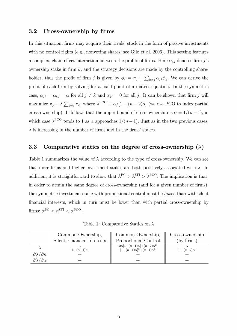
3.3 Comparative statics on the degree of cross-ownership (�)

Table 1 summarizes the value of � according to the type of cross-ownership. We can see

that more �rms and higher investment stakes are both positively associated with �. In

addition, it is straightforward to show that �PC > �SFI > �PCO. The implication is that,

in order to attain the same degree of cross-ownership (and for a given number of �rms),

the symmetric investment stake with proportional control must be lower than with silent

�nancial interests, which in turn must be lower than with partial cross-ownership by

�rms: �PC < �SFI < �PCO.

Table 1: Comparative Statics on �

Common Ownership,Silent Financial Interests

Common Ownership,Proportional Control

Cross-ownership(by �rms)

� �1�(n�1)�

2�[1�(n�1)�]+(n�2)�2[1�(n�1)�]2+(n�1)�2

�1�(n�2)�

@�=@n + + +@�=@� + + +

9

4 Framework and equilibrium

We consider an industry consisting of n � 2 identical �rms, where each �rm i = 1; : : : ; n

chooses simultaneously their R&D intensity (xi) and production quantity (qi). Firms

produce a homogeneous good characterized by a smooth inverse demand function f(Q),

where Q =P

i qi. We make the following three assumptions.

A.1. f(Q) is twice continuously di¤erentiable, where (i) f 0(Q) < 0 for all Q � 0 such

that f(Q) > 0 and (ii) the elasticity of the slope of the inverse demand function,

�(Q) � Qf 00(Q)

f 0(Q);

is constant and equal to �.

The parameter � is the curvature (relative degree of concavity) of the inverse demand

function, so demand is concave for � > 0 and is convex for � < 0. Furthermore, demand

is log-concave for 1 + � > 0 and is log-convex for 1 + � < 0. If 1 + � = 0, then demand is

both log-concave and log-convex.12 Assumption A.1 is always satis�ed by inverse demand

functions that are linear or constantly elastic. In particular, the family of inverse demand

functions for which �(Q) is constant can be represented as

f(Q) =

8><>:a� bQ�+1 if � 6= �1;

a� b logQ if � = �1;

here a is a nonnegative constant and b > 0 (resp., b < 0) if � � �1 (resp., � < �1).

A.2. The marginal production cost or innovation function of �rm i, or ci, is independent

of output and is decreasing in both own and rivals�R&D as follows: ci = c(xi+�P

j 6=i xj),

where c0 < 0, c00 � 0, and 0 � � � 1 for i 6= j.

A.3. The cost of investment is given by the function �(xi), where �(0) = 0, �0 > 0, and

�00 � 0.12We remark that � is also related to the marginal consumer surplus from increasing output� that is,

to MS = �f 0(Q)Q. After setting �MS as the elasticity of the inverse marginal consumer surplus function(so that �MS = MS=(MS

0Q)), Weyl and Fabinger (2013) argue that �MS measures the curvature of thelogarithm of demand. Under A.1, we can write 1=�MS = 1 + �.

10

The parameter � represents the spillover level of the R&D activity. Since we focus on

symmetric �rms, we assume symmetric spillover levels; moreover, R&D outcomes are

imperfectly appropriable to an extent that varies between 0 and 1.13

Firm i�s pro�t is given by

�i = f(Q)qi � c

�xi + �

Xj 6=i

xj

�qi � �(xi);

and the objective function for �rm i is �i = �i+�P

k 6=i �k (i.e., equation (1)). The model

represents distinct scenarios depending on the values of � and �. When � 2 (0; 1) and

� 2 [0; 1), �rms compete in the presence of partial ownership interests and the R&D

outcomes are again imperfectly appropriable. When � 2 (0; 1) and � = 1, �rms form

a Research Joint Venture under which all R&D outcomes are fully shared among RJV

members and the duplication of R&D e¤orts is avoided. When � = � = 1, �rms form a

�cartelized�RJV. If � = 0 then there are no minority interests.

For markets with cross-shareholdings, a modi�ed HHI is proposed by Bresnahan and

Salop (1986). This index corresponds to the market share�weighted Lerner index in a

Cournot market, and we writeMHHI =�P

i siLi��. Here si and Li are (respectively) the

market share and Lerner index of �rm i; the term � denotes the demand price elasticity).14

In our case it is easy to see that, for a given common marginal cost, (p� c)=p = MHHI=�

at a symmetric Cournot equilibrium; here MHHI = �=n for � = 1 + �(n � 1), which is

monotone in �. When � = 0 we have the standard HHI for a symmetric solution, 1=n,

and if � = 1 then the modi�ed HHI is equal to 1.

Now we consider symmetric solutions. Let B = 1+�(n�1); then Bx is the �e¤ective�

investment that lowers costs for a �rm. Let � = 1 + �(n � 1)�. Then �c0(Bx)q� is

the marginal e¤ect of invesment by a �rm on its internalized pro�t �i. A symmetric

interior equilibrium (Q� = nq�; x�) must solve the �rst-order necessary conditions for the

13The intensity of the spillover e¤ects is heterogeneous across industries, which could be due to anegative relationship between spillovers and patent protection levels. That is, industries with low patentprotection tend to have higher spillover levels than do industries with high patent protection (Griliches1990).14Azar et al. (2015) use the MHHI (in terms of control and share rights) to measure anticompetitive

incentives stemming from �nancial interests in the US airline industry. These authors �nd that, in year2013, the market concentration generated by such �nancial interests was more than 10 times greaterthan the HHI changes above which mergers are likely to generate antitrust concerns.

11

maximization of �i:

f(Q�)� c(Bx�)

f(Q�)=MHHI�(Q�)

; (2)

�c0(Bx�)Q��

n= �0(x�): (3)

Here �(Q�) = �f(Q�)=(Q�f 0(Q�)) is the elasticity of demand. Equation (2) is the mod-

i�ed Cournot�Lerner pricing formula; expression (3) equates the marginal bene�t and

marginal cost of invesment by a �rm with its internalized pro�t �i. Note that both MHHI

and � are increasing in � and therefore respectively exert pressure to reduce output (or

increase prices and margins) and to increase investment.

Let second-order derivatives and cross-derivatives be de�ned, at symmetric solutions,

by @zz�i � @2�i=@z2i , @zi;j�i � @2�i=@zi@zj, @hz�i � @2�i=@h@zi (with h = �, �, and

z = q; x), and @xq�i � @2�i=@xi@qi (i 6= j; i; j = 1; 2; : : : ; n).15 We assume that the

following stability conditions hold:

�q � @qq�i + (n� 1)@qi;j�i < 0;

�x � @xx�i + (n� 1)@xi;j�i < 0;

and

� � �q�x � (@xq�i)2�B > 0: (4)

Together these conditions imply that (2) and (3) both have a unique solution. It is note-

worthy that �x < 0 requires that at least one of c00 and �00 be positive (see Table 7 in

Appendix A). If �(Q�; x�) > 0 then we say that the equilibrium is regular ; the ratio-

nale for this terminology will become clear in the comparative statics analysis to follow.

In particular, we assume that there is a unique regular symmetric interior equilibrium

(Q�; x�). The focus of our paper is on characterizing that equilibrium.

4.1 Model speci�cation examples

We will consider the well-known R&D model speci�cations� with linear (and there-

fore log-concave) demand� of d�Aspremont�Jacquemin (AJ) and Kamien�Muller�Zang

(KMZ); we also consider a constant elasticity (CE) model with log-convex demand that

15See Table 7 in Appendix A for the full expressions of these variables.

12

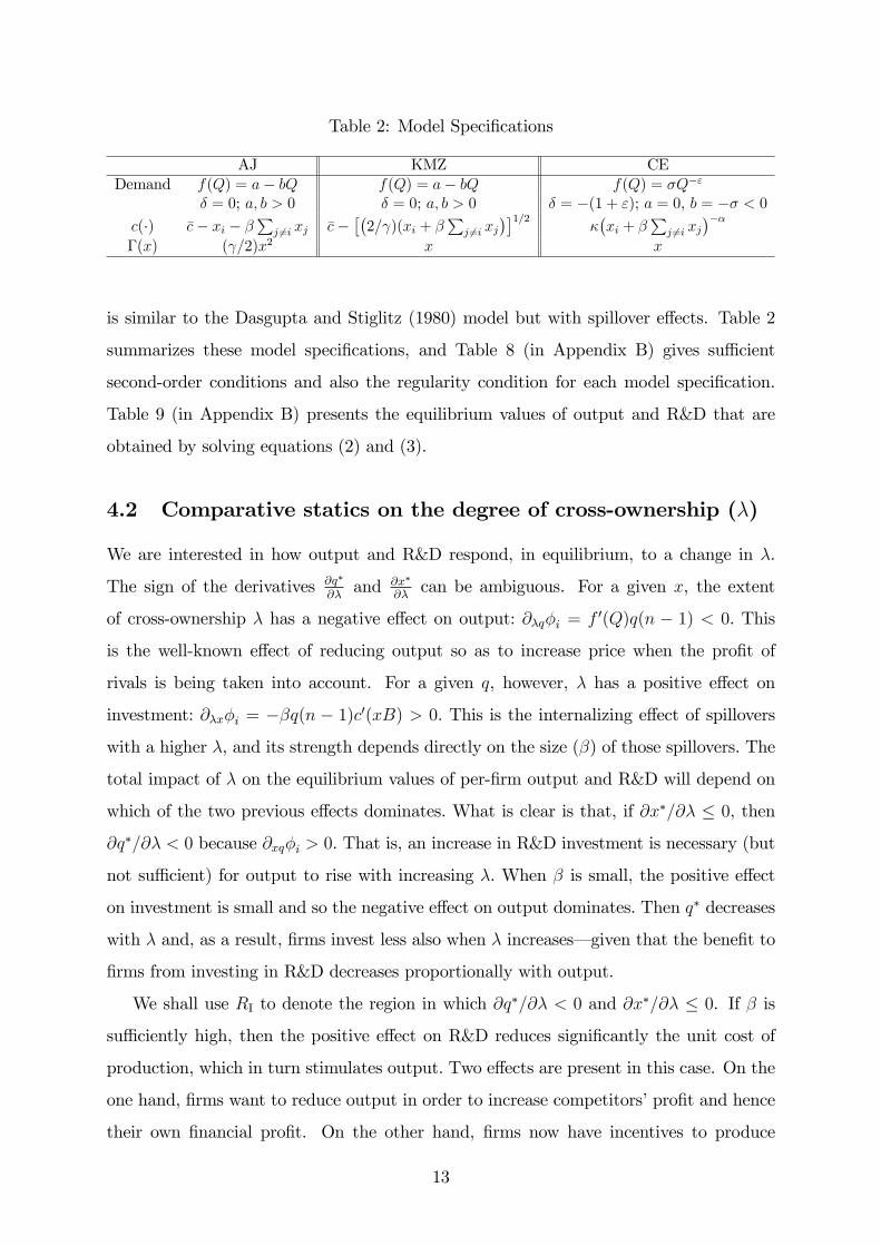
Table 2: Model Speci�cations

AJ KMZ CEDemand f(Q) = a� bQ f(Q) = a� bQ f(Q) = �Q�"

� = 0; a; b > 0 � = 0; a; b > 0 � = �(1 + "); a = 0, b = �� < 0c(�) �c� xi � �

Pj 6=i xj �c�

��2= )(xi + �

Pj 6=i xj

��1=2��xi + �

Pj 6=i xj

��(x) ( =2)x2 x x

is similar to the Dasgupta and Stiglitz (1980) model but with spillover e¤ects. Table 2

summarizes these model speci�cations, and Table 8 (in Appendix B) gives su¢ cient

second-order conditions and also the regularity condition for each model speci�cation.

Table 9 (in Appendix B) presents the equilibrium values of output and R&D that are

obtained by solving equations (2) and (3).

4.2 Comparative statics on the degree of cross-ownership (�)

We are interested in how output and R&D respond, in equilibrium, to a change in �.

The sign of the derivatives @q�

@�and @x�

@�can be ambiguous. For a given x, the extent

of cross-ownership � has a negative e¤ect on output: @�q�i = f 0(Q)q(n � 1) < 0. This

is the well-known e¤ect of reducing output so as to increase price when the pro�t of

rivals is being taken into account. For a given q, however, � has a positive e¤ect on

investment: @�x�i = ��q(n � 1)c0(xB) > 0. This is the internalizing e¤ect of spillovers

with a higher �, and its strength depends directly on the size (�) of those spillovers. The

total impact of � on the equilibrium values of per-�rm output and R&D will depend on

which of the two previous e¤ects dominates. What is clear is that, if @x�=@� � 0, then

@q�=@� < 0 because @xq�i > 0. That is, an increase in R&D investment is necessary (but

not su¢ cient) for output to rise with increasing �. When � is small, the positive e¤ect

on investment is small and so the negative e¤ect on output dominates. Then q� decreases

with � and, as a result, �rms invest less also when � increases� given that the bene�t to

�rms from investing in R&D decreases proportionally with output.

We shall use RI to denote the region in which @q�=@� < 0 and @x�=@� � 0. If � is

su¢ ciently high, then the positive e¤ect on R&D reduces signi�cantly the unit cost of

production, which in turn stimulates output. Two e¤ects are present in this case. On the

one hand, �rms want to reduce output in order to increase competitors�pro�t and hence

their own �nancial pro�t. On the other hand, �rms now have incentives to produce

13

more because they are more e¢ cient. If the �rst e¤ect dominates, then @q�=@� < 0

and @x�=@� > 0 (we label this region RII). But if the second e¤ect dominates, then

@q�=@� > 0 and @x�=@� > 0 (region RIII). Which of these two cases arises in equilibrium

will depend on the extent of the spillovers. We �nd that, whereas RI always exists, regions

RII and RIII might not exist.

We next derive the conditions and threshold values (in terms of �) that de�ne the

boundaries of the regions characterizing the signs of @x�=@� (Lemma 1) and @q�=@�

(Lemma 2).

LEMMA 1 At equilibrium,

sign

�@x�

@�

�= signf�(1 + n+ ��)� 1g:

COROLLARY 1 For any �xed � and for any � 2 [0; 1]; only RI exists (with @x�=@� � 0)

if and only if demand is convex enough� that is, i¤ � � �n=�.16 This statement holds

for any � in the interval [0; 1] provided that � � �n.

We can interpret the critical spillover threshold for � in terms of the cost pass-through

coe¢ cient (i.e., the rate at which the price changes with marginal cost). This threshold is

equal to the industry-wide per-�rm cost pass-through coe¢ cient (P 0(c)=n) multiplied by

the internalized cost-reducing e¤ect of a unit increase in R&D expenditures by a �rm (�);

formally, we have sign�@x�

@�

= signf��P 0(c)�=ng. Note that the threshold is decreasing

in the pass-through coe¢ cient because �rms are less interested in reducing costs when

doing so translates, in e¤ect, into lower prices.17

A consequence of Lemma 1 is that the threshold for spillovers to induce @x�=@� � 0 is

decreasing (resp. increasing) in � when demand is concave (resp. convex)� that is, when

� > 0 (resp. � < 0). So for � > 0, if @x�=@� > 0 for some � then that inequality must

hold also for larger values of �. Analogously: for � < 0, if @x�=@� < 0 for some � then

that inequality holds also for larger values of �.

If demand is extremely convex, then increases in cross-ownership are so restrictive

of output that they induce @x�=@� < 0, in which case only RI exists for any �. And

16When � > �(n+1)=�, there exists a positive threshold of spillover above which @x�=@� > 0; however,that threshold exceeds unity unless � > �n=�.17Let P (c) � f(nq�(c)); then P 0(c) = f 0(nq�)n

�dq�

dc

�= n

�(1+�)+n . Since the stability condition �q < 0holds when �(1 + �) + n > 0, it follows that P 0(c) > 0. Furthermore, the pass-through increases withthe number of �rms when demand is log-concave (� > �1). See, for example, Weyl and Fabinger (2013).

14

since MHHI = �=n, the applicable condition is that � � �(MHHI)�1. Corollary 1

implies that the degree of demand convexity required for only RI to exist is decreasing

in the concentration measured by MHHI; in other words, the condition is less restrictive

in markets that are more concentrated. The corollary implies also that RII can exist

only when quantities are strategic substitutes. Indeed, if quantities are instead strategic

complements (i.e.., if @qi;j�i > 0, which holds when � < �n(1+�)=�), then the condition

� < �n=� also holds and only RI exists. When � is such that �n(1 + �)=� < � < �n=�,

quantities are strategic substitutes (as e.g. when demand is log-concave) but again only

RI exists. If � > �n=�, then quantities are strategic substitutes and so RII exists (see

Figure 8 in Appendix A).

As regards the comparative statics on output, totally di¤erentiating the �rst-order

condition (FOC) with respect to � yields

sign

�@q�

@�

�= sign

�@�q�i + (@xq�i)B

@x�

@�

�; (5)

here B = 1+�(n� 1) captures the e¤ect, on each �rm�s marginal cost, of a unit increase

in R&D by all �rms. At equilibrium, the impact on output of a higher degree of cross-

ownership depends directly on its e¤ect on marginal pro�t with respect to output (@�q�i)

and indirectly through its e¤ect on the R&D e¤ort of each �rm at equilibrium. Recall

that, since @xq�i > 0, it follows that if @x�=@� � 0 then @q�=@� < 0 (RI). By Lemma 1

we know that, if spillovers are su¢ ciently high, then @x�=@� > 0; however, the sign of

@q�=@� can be negative (RII) or positive (RIII).

We derive an inverse measure of R&D e¤ectiveness in terms of the model�s basic

elasticities. This measure H is a function of � and provides the appropriate threshold

for the positive e¤ect of minority shareholdings on R&D investments to dominate its

negative e¤ect on output. Let �(Bx�) � �c00(Bx�)Bx�=c0(Bx�) � 0 be the elasticity of

the slope of the innovation function (i.e., the relative convexity of c(�)) evaluated at the

e¤ective R&D, Bx�; and let y(x�) � �00(x�)x�=�0(x�) � 0 be the elasticity of the slope

of the investment cost function. Our regularity assumptions imply that either c00 > 0

or �00 > 0 (or both). If �00(x�) > 0, let �(Q�; x�) � ��(c0(Bx�))2=(f 0(Q�)�00(x�)) > 0

measure the relative e¤ectiveness of R&D,18 weighted by �. Then H can be written as

18As de�ned by Leahy and Neary (1997, Sec. V, p. 654).

15

H =1

�(Q�; x�)

�1 +

�(Bx�)

y(x�)

�;

evaluated at the equilibrium (Q�; x�) for � > 0. Note that lim�!0H =1.

LEMMA 2 Let B = 1 + �(n� 1). At equilibrium,

sign

�@q�

@�

�= signfB �Hg: (6)

Just as it does for �, the term H provides the appropriate threshold for B, or the

e¤ect (on each �rm�s marginal cost) of a unit increase in R&D by all �rms. Therefore, if

B > H then the positive e¤ect of minority shareholdings on R&D investments dominates

its negative e¤ect on output. At equilibrium, a higher degree of cross-ownership increases

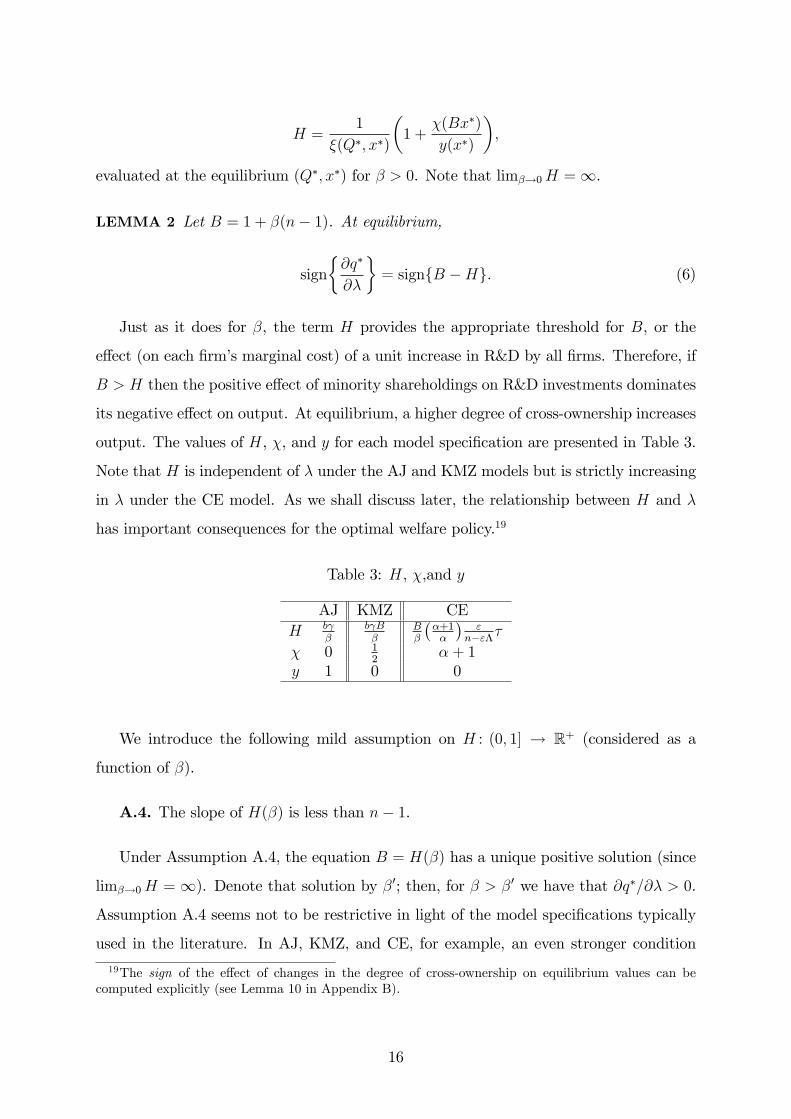
output. The values of H, �, and y for each model speci�cation are presented in Table 3.

Note that H is independent of � under the AJ and KMZ models but is strictly increasing

in � under the CE model. As we shall discuss later, the relationship between H and �

has important consequences for the optimal welfare policy.19

Table 3: H, �,and y

AJ KMZ CEH b

�b B�

B�

��+1�

�"

n�"��

� 0 12

�+ 1y 1 0 0

We introduce the following mild assumption on H : (0; 1] ! R+ (considered as a

function of �).

A.4. The slope of H(�) is less than n� 1.

Under Assumption A.4, the equation B = H(�) has a unique positive solution (since

lim�!0H = 1). Denote that solution by �0; then, for � > �0 we have that @q�=@� > 0.

Assumption A.4 seems not to be restrictive in light of the model speci�cations typically

used in the literature. In AJ, KMZ, and CE, for example, an even stronger condition

19The sign of the e¤ect of changes in the degree of cross-ownership on equilibrium values can becomputed explicitly (see Lemma 10 in Appendix B).

16

holds� namely, that H(�)=B is strictly decreasing in �. Assumption A.4 does not guar-

antee that �0 < 1, so RIII may fail to exist. We have that �0 < 1 if n > H(1). Our next

corollary states the results formally.

COROLLARY 2 Under A.4, if n > H(1) then region RIII exists when � > �0 with �0 < 1

(where �0 is the unique positive solution to B �H(�) = 0).

Using Lemmas 1 and 2� and observing that � > �n=� implies that 1+n+�� > 0� we

obtain the following result.

PROPOSITION 1 Let � = 1 + �(n � 1). Under assumptions A.1�A.3, if demand is

su¢ ciently convex (� � �n=�) then only region RI exists. Otherwise, assume A.4 and

let �0 be the unique positive solution of B = H(�). Then the following statements hold :

(i) if � � 1=(1 + n+ ��); then @x�

@�� 0 and @q�

@�< 0 (RI);

(ii) if 1=(1 + n+ ��) < � � �0; then @q�

@�� 0 and @x�

@�> 0 (RII);

(iii) if � > �0; then @q�

@�> 0 and @x�

@�> 0 (RIII).

This proposition implies that, for demand that is convex enough, the equilibrium is

always in RI. Otherwise, the equilibrium is in RI for only a low level of spillovers. It

is instructive to compare these results with those reported by Leahy and Neary (1997,

Prop. 3), in which there are no minority shareholdings and where R&D cooperation leads

to more R&D and output (as in our RIII) whenever spillovers are positive. Yet in our case,

RIII obtains only when spillovers are su¢ ciently high. Thus the �output cooperation�

induced by minority shareholdings requires su¢ ciently high spillovers in order to increase

R&D and output.

Finally, we are interested in analyzing the e¤ect of � on each �rm�s pro�t. We have

that

signf��0(�)g = sign�� c0(Bx�)

@x�

@�+ f 0(Q�)

@q�

@�

�: (7)

Given that @x�=@� > 0 and @q�=@� < 0 in RII, we can use (7) to show that� in this

region� ��0(�) > 0. The sign of the e¤ect of � on �� is less clear in RI (since in that

region, @x�=@� < 0 and @q�=@� < 0) and in RIII (where @x�=@� > 0 and @q�=@� > 0).

Nevertheless, in Appendix B we prove the following result.

17

PROPOSITION 2 At the symmetric equilibrium, the pro�t per �rm (��) increases with �.

According to this proposition, the positive e¤ect on price dominates the negative e¤ect

on R&D in RI, and conversely in RIII, so that pro�ts in both regions rise with the extent

of cross-ownership. Hence �rms are incentivized to acquire (minority) shareholdings in

the industry� provided the agreements they enter are binding ones, because that feature

allows them to increase pro�ts.20 Before proceeding with the welfare analysis, we examine

the e¤ect of � on equilibrium values.

4.3 Comparative statics on spillovers (�)

A su¢ cient (but not necessary) condition for increases in � to raise per-�rm R&D and

output is that @�x�i > 0. It is not di¢ cult to see that signf@�x�ig = signf�B=��(Bx�)g;

here � is the elasticity of the slope of the innovation function, which is nonnegative. For

a positive �, we have @�x�i > 0 when the curvature (relative convexity) of the innovation

function is su¢ ciently low. The term �B=� increases with �, so it su¢ ces that � < �

(since B=� = 1 for � = 0). Our next proposition follows.

PROPOSITION 3 If the curvature � of the innovation function is su¢ ciently low (� <

� would be low enough); then @q�=@� > 0 and @x�=@� > 0.

We can view the following results as corollaries. In AJ (where � = 0), stronger spillover

e¤ects raise the equilibrium values of output and R&D; in KMZ (where � = 1=2), the

same dynamic is observed when cross-ownership induces a high enough � (� > 1=2) and

always in the case of a cartel (for which � = 1). In the CE model, � = � + 1 > 1.

In this case, some tedious algebra shows that, for any positive �, (i) @q�=@� > 0 (with

@q�=@� = 0 when � = 0) and (ii) x� increases (resp. decreases) with � for high (resp.

low) values of �.

20Farrell and Shapiro (1990), Flath (1991), and Reitman (1994) show that unilateral incentives toimplement passive ownership structures may be lacking in Cournot competition with constant marginalcosts. However, Gilo et al. (2006) show that cross-ownership arrangements facilitate tacit collusion (inthe symmetric case) when the stakes are su¢ ciently high. For a di¤erentiated product market with two�rms, Karle et al. (2011) analyze the incentives of an investor to acquire a controlling or noncontrollingstake in a competitor.

18

5 Welfare analysis

Welfare in equilibrium is given by the sum of consumer surplus and industry pro�ts:

W (�) =

Z Q�

0

f(Q) dQ� c(Bx�)Q� � n�(x�):

We are interested in studying the e¤ect of � on welfare. Using the equilibrium condi-

tions (2) and (3), we can write

W 0(�) =

�� f 0(Q�)@q

�

@�� (1� �)�(n� 1)c0(Bx�)@x

�

@�

�Q�: (8)

An increase in cross-ownership alters equilibrium values of quantities and R&D invest-

ments, and each additional unit of output and R&D has social value equal to (respectively)

�(�f 0(Q�))Q� and (1� �)�(n� 1)(�c0(Bx�))Q�. Here Proposition 1 is useful. In RI we

have that W 0(�) < 0 because @x�=@� � 0 and @q�=@� < 0; in RIII, W 0(�) > 0 because

@x�=@� > 0 and @q�=@� > 0. In RII, however, the e¤ect of � on welfare is positive or

negative according as whether the positive e¤ect of minority shareholdings on R&D does

or does not dominate its negative e¤ect on output level. Moreover, from

signfCS0(�)g = sign�@q�

@�

�(9)

it follows that the e¤ect of � on consumer surplus is positive (i.e., CS0(�) > 0) only in

RIII. So even as consumers su¤er from a higher degree of cross-ownership RI and RII, it

bene�ts them in RIII. One consequence is that optimal antitrust policy will tend to be

stricter under the CS standard.

5.1 Socially optimal degree of cross-ownership

Let �oCS and �oTS denote the optimal degree of cross-ownership under the (respectively)

consumer surplus and total surplus standard. Let �0(�) denote the dependence of �0

on �. Then it is easy to see that H is increasing in � if and only if �0(�) is also increasing

in �. Recall that H is weakly increasing in � under the all three model speci�cations:

in AJ and KMZ, H is independent of �; in the CE model, H is strictly increasing in �.

19

Furthermore, in these three speci�cationsW (�) is single peaked:21 a mild additional con-

dition is required in KMZ (as we discuss later). In the CE model, numerical simulations

show that� for the parameter range in which the second-order condition (SOC) and the

regularity condition are satis�ed�W (�) is strictly concave.

We know from Proposition 1 that if demand is convex enough then only RI exists, in

which case no cross-ownership is optimal regardless of spillover levels. Otherwise (and

under some mild assumptions): if spillovers � are low enough then cross-ownership is

also not optimal; and if spillovers are high enough then the degree of cross-ownership

should be positive in terms of both total surplus and consumer surplus (i.e., �oTS > 0 and

�oCS > 0). For intermediate values of � we have that �oTS > �oCS = 0. It follows that more

cross-ownership should be allowed under the total surplus standard (i.e., �oTS � �oCS).

These results are stated formally in our next proposition.

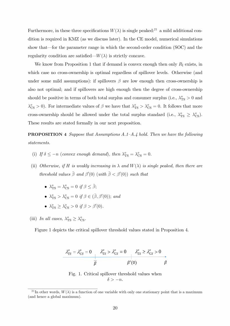
PROPOSITION 4 Suppose that Assumptions A.1�A.4 hold. Then we have the following

statements.

(i) If � � �n (convex enough demand); then �oTS = �oCS = 0.

(ii) Otherwise, if H is weakly increasing in � and W (�) is single peaked, then there are

threshold values �� and �0(0) (with �� < �0(0)) such that

� �oTS = �oCS = 0 if � � ��;

� �oTS > �oCS = 0 if � 2 (��; �0(0)); and

� �oTS � �oCS > 0 if � > �0(0).

(iii) In all cases, �oTS � �oCS.

Figure 1 depicts the critical spillover threshold values stated in Proposition 4.

Fig. 1. Critical spillover threshold values when� > �n.

21In other words, W (�) is a function of one variable with only one stationary point that is a maximum(and hence a global maximum).

20

Remark 1. We have that �� < 1 if n+(n�1)(�+n) > H(1) (see Lemma 6 in Appendix A).

If �� 1 then �oTS = �oCS = 0 for all � � 1.

Remark 2. Our single-peakedness assumption on W (�) ensures that �� is the minimum

threshold above which total surplus increases with � (i.e., for which � � �� implies

�oTS = 0).

Remark 3. The assumption that H is weakly increasing in � ensures that � < �0(0)

implies �oCS = 0 and that �oTS � �oCS. In the particular case where � = �0(0) we have that

�oTS � �oCS � 0 (see the proof of Proposition 4 in Appendix A).

If we relax the assumptions that W (�) be single peaked and that H be monotonic in �,

then we can provide a weaker characterization of the regions where cross-ownership is

socially optimal (Proposition 5) and can also characterize the extreme solution regions

where �oCS = 0 or �oCS = �oTS = 1 (Proposition 6).

PROPOSITION 5 Let A.1�A.4 hold. If � > �(1+n)=n; then there exist threshold values

� < �� < �0(0) (where � = inff1=(1 + n + ��) : � 2 [0; 1]g) such that : (i) �oCS = �oTS = 0

for � � �; (ii) �oTS > 0 for � > ��; and (iii) �oCS > 0 for � > �0(0).

From Proposition 1 it now follows that, when � � �, only RI exists because � >

�(1 + n)=n implies that 1 + n + �� > 0 and � > �n. The threshold � depends on the

sign of �. If demand is concave (� > 0), then � = 1=(1 + n(1 + �)); if demand is convex

(� < 0), then � = 1=(1 + n + �). In both cases, � decreases with n (and tends to 0

with n).22 Parts (ii) and (iii) follow as in Proposition 4: part (ii) because if � > �� then

W 0(0) > 0 and so �oTS > 0; and part (iii) because if � > �0(0) then @q�=@�j�=0 > 0 and

�oCS > 0. (See Appendix B for details.)

PROPOSITION 6 Under A.1�A.4, the following statements hold :

(i) � � �0min implies �oCS = 0; and

(ii) � > �0max implies �oCS = �oTS = 1 provided that �

0max � 1.

22In AJ and KMZ, demand is linear; hence � = 1=(1 + n). Under CE, � < 0 when " > �1 and so� = 1=(n� "); in contrast, � = 1=(1� n") when " < �1.

21

This proposition is proved by noting that �0(�) is a continuous function on [0; 1] and

so achieves a maximum (�0max) and a minimum (�0min) within that interval. If � � �0min,

then @q�=@� < 0 for all � > 0 and so �oCS = 0; if � > �0max, then @q�=@� > 0 for all �.

Since @q�=@� > 0 implies @x�=@� > 0 by equation (5), it follows that W 0(�) > 0 for all

� by equation (8). Therefore, �oCS = �oTS = 1 provided that �0max � 1.

We can now make the following claims. (a) If H is strictly decreasing in �, then �0(�)

also is: �0min = �0(1) and �0max = �0(0). (b) If H is strictly increasing in �, then �0(�)

also is: �0min = �0(0) and �0max = �0(1). (c) If H is independent of �, then �0 also is:

�0min = �0max = �0.

Proposition 6 determines when the monopoly outcome (� = 1) is optimal in terms of

both consumer and total surplus (in those cases, we are in RIII and welfare is increasing

in �). In AJ and KMZ, the term H is independent of �; thus case (c) applies and, as a

result, the consumer surplus solution is bang-bang under either model speci�cation. In

both speci�cations it is clear that if �oCS > 0 then necessarily �oTS = �oCS = 1. In the

CE model, however, H and �0 are strictly increasing in � and so case (b) applies; hence

solutions of the form �oTS > �oCS > 0 are possible.23

The scope for a Research Joint Venture.

An RJV can be understood as a situation where spillovers are fully internalized (i.e.,

� = 1). If the RJV is �cartelized� then also � = 1. This arrangement can be optimal

only if RIII exists for � large (with �0max � 1) and if @q�=@� > 0 and @x�=@� > 0 (which,

by Proposition 3, requires that � < 1). Our next corollary states the result.

COROLLARY 3 Again assume that A.1�A.4 hold. If �0max � 1 and if the innovation

function�s curvature is not too large (� < 1); then a cartelized RJV (� = � = 1) is optimal

in terms of consumer surplus and welfare.

The assumptions of the corollary are ful�lled in the AJ and KMZ models, where

b < n and b < 1 are needed (respectively) to ensure that �0AJ and �0KMZ are less

than unity; recall that � = 0 in AJ and � = 1=2 in KMZ. In CE, � = 1 is never socially

optimal because �0CE(1) < 1 only if " < �=(1+2�)� which would contradict the regularity

condition (see Table 8 in Appendix B).

23In the proof of Proposition 4 we show that, in the CE case, CS is globally concave in � whenB > H(�)j�=0. Letting �� denote the unique value for � such that @q�=@� = 0, we have that ��CS = 1when �� > 1; hence ��CS = minf��; 1g, which yields ��TS > ��CS > 0.

22

Under some di¤erent conditions, an RJV with no cross-ownership (� = 0 and � =

1) can be socially optimal in all three models (see Proposition 7 in Appendix B). To

determine when an RJV with no cross-ownership is socially optimal, we use that� when

W (�) is single peaked� �� is the minimum threshold above which allowing some cross-

ownership increases welfare (Proposition 4), so no cross-ownership is optimal if �� 1.

Satisfying that inequality requires b � n2 in AJ, b � n in KMZ, and a more involved

condition in CE. In contrast with the AJ model, in both KMZ and CE we �nd that if

� = 0 then greater R&D spillovers reduce R&D expenditures (@x�=@� < 0) while having

no e¤ect on output (@q�=@� = 0). Although R&D expenditures are lower with higher �,

the production costs of all �rms are also lower. In both cases, the greater R&D spillover�s

negative e¤ect on R&D expenditures is dominated by its positive e¤ect on the innovation

function; as a result, � = 1 is also socially optimal.

5.2 Comparative statics by model

We are interested in the comparative statics of the regions determining the scope for

cross-ownership as described in Proposition 4. We are also interested in the comparative

statics on �oCS and �oTS in the speci�ed models.

Comparative statics on �0. Table 4 summarizes the comparative static results on

�0(0) in the models with respect to basic parameters. The threshold �0(0) is weakly

decreasing in n and is strictly decreasing in demand elasticity; however, the e¤ect of the

innovation function�s elasticity is ambiguous. In terms of consumer surplus, in AJ it is

optimal to suppress minority shareholdings for any level of spillovers when �rm entry is

insu¢ cient� that is, when n < b (since then �0AJ > 1); in CE, suppression is optimal

when n < "(2�+ 1)=� (since �0CE > 1 for n < "(2�+ 1)�=�).24

Table 10 (in Appendix B) reports the spillover thresholds for AJ, KMZ and CE

models. To obtain some further insights into the comparative statics on the spillover

threshold �� and on the socially optimal degree of cross-ownership, we conducted some

numerical simulations.25 The results are described next.24In AJ, @H=@n = 0 and so increasing the number of �rms reduces the �0 threshold (@�0AJ=@n < 0);

in KMZ, however, �rm entry has no e¤ect on �0 (@�0KMZ=@n = 0). In the CE model, the direction ofthe e¤ect of entry on the �0 threshold depends on the value of �. In particular, �0CE decreases (resp.increases) with n when � is low (resp. high).25Values for parameters are chosen so that the regularity condition and the SOCs are satis�ed.

23

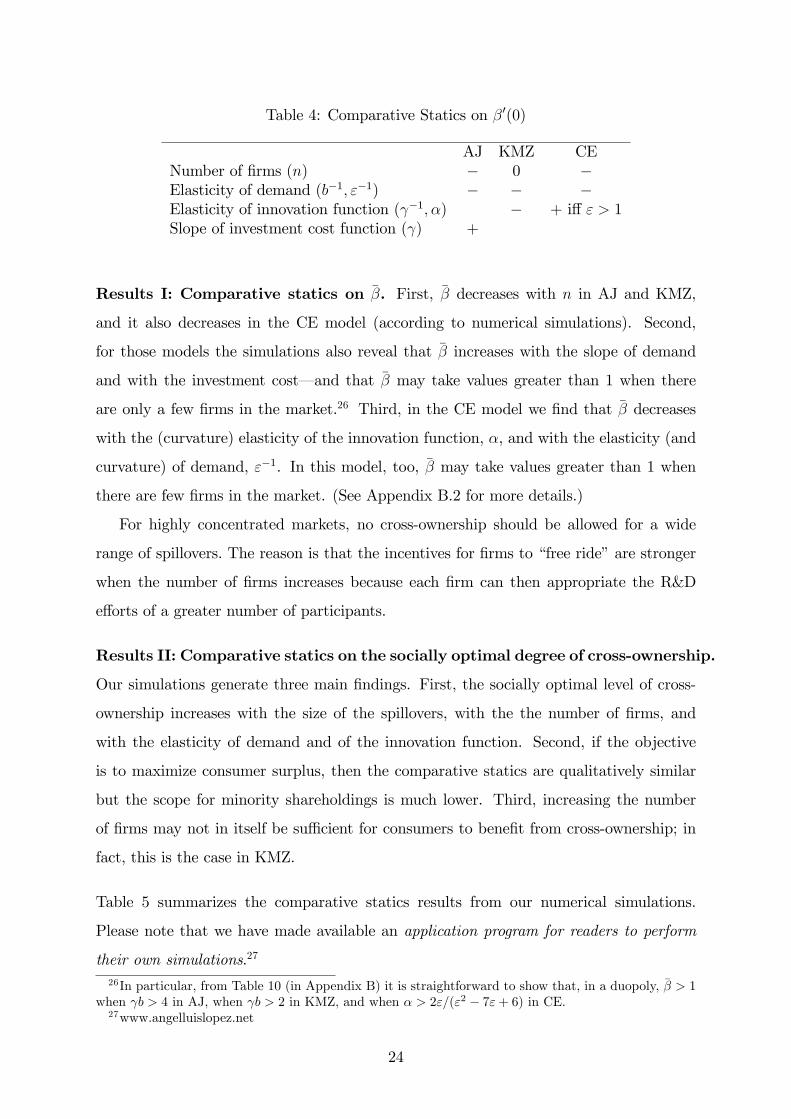
Table 4: Comparative Statics on �0(0)

AJ KMZ CENumber of �rms (n) � 0 �Elasticity of demand (b�1; "�1) � � �Elasticity of innovation function ( �1; �) � + i¤ " > 1Slope of investment cost function ( ) +

Results I: Comparative statics on ��. First, �� decreases with n in AJ and KMZ,

and it also decreases in the CE model (according to numerical simulations). Second,

for those models the simulations also reveal that �� increases with the slope of demand

and with the investment cost� and that �� may take values greater than 1 when there

are only a few �rms in the market.26 Third, in the CE model we �nd that �� decreases

with the (curvature) elasticity of the innovation function, �, and with the elasticity (and

curvature) of demand, "�1. In this model, too, �� may take values greater than 1 when

there are few �rms in the market. (See Appendix B.2 for more details.)

For highly concentrated markets, no cross-ownership should be allowed for a wide

range of spillovers. The reason is that the incentives for �rms to �free ride�are stronger

when the number of �rms increases because each �rm can then appropriate the R&D

e¤orts of a greater number of participants.

Results II: Comparative statics on the socially optimal degree of cross-ownership.

Our simulations generate three main �ndings. First, the socially optimal level of cross-

ownership increases with the size of the spillovers, with the the number of �rms, and

with the elasticity of demand and of the innovation function. Second, if the objective

is to maximize consumer surplus, then the comparative statics are qualitatively similar

but the scope for minority shareholdings is much lower. Third, increasing the number

of �rms may not in itself be su¢ cient for consumers to bene�t from cross-ownership; in

fact, this is the case in KMZ.

Table 5 summarizes the comparative statics results from our numerical simulations.

Please note that we have made available an application program for readers to perform

their own simulations.27

26In particular, from Table 10 (in Appendix B) it is straightforward to show that, in a duopoly, �� > 1when b > 4 in AJ, when b > 2 in KMZ, and when � > 2"=("2 � 7"+ 6) in CE.27www.angelluislopez.net

24

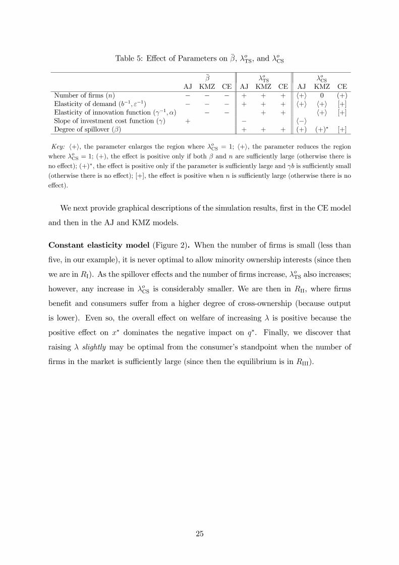
Table 5: E¤ect of Parameters on ��, �oTS, and �oCS

�� oTS �oCSAJ KMZ CE AJ KMZ CE AJ KMZ CE

Number of �rms (n) � � � + + + h+i 0 (+)Elasticity of demand (b�1; "�1) � � � + + + h+i h+i [+]Elasticity of innovation function ( �1; �) � � + + h+i [+]Slope of investment cost function ( ) + � h�iDegree of spillover (�) + + + (+) (+)� [+]

Key: h+i, the parameter enlarges the region where �oCS = 1; h+i, the parameter reduces the regionwhere �oCS = 1; (+), the e¤ect is positive only if both � and n are su¢ ciently large (otherwise there is

no e¤ect); (+)�, the e¤ect is positive only if the parameter is su¢ ciently large and b is su¢ ciently small

(otherwise there is no e¤ect); [+], the e¤ect is positive when n is su¢ ciently large (otherwise there is no

e¤ect).

We next provide graphical descriptions of the simulation results, �rst in the CE model

and then in the AJ and KMZ models.

Constant elasticity model (Figure 2). When the number of �rms is small (less than

�ve, in our example), it is never optimal to allow minority ownership interests (since then

we are in RI). As the spillover e¤ects and the number of �rms increase, �oTS also increases;

however, any increase in �oCS is considerably smaller. We are then in RII, where �rms

bene�t and consumers su¤er from a higher degree of cross-ownership (because output

is lower). Even so, the overall e¤ect on welfare of increasing � is positive because the

positive e¤ect on x� dominates the negative impact on q�. Finally, we discover that

raising � slightly may be optimal from the consumer�s standpoint when the number of

�rms in the market is su¢ ciently large (since then the equilibrium is in RIII).

25

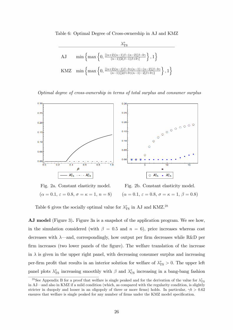
Table 6: Optimal Degree of Cross-ownership in AJ and KMZ

�oTS

AJ minnmax

n0; [(n+2)(n�1)��(n�2)]��b

(n�1)[2(��1)�+b ]

o; 1o

KMZ minnmax

n0; [(n+2)(n�1)��b (n�1)�(n�2)]��b

(n�1)f[2�+b (n�1)�2]�+b g

o; 1o

Optimal degree of cross-ownership in terms of total surplus and consumer surplus

Fig. 2a. Constant elasticity model.

(� = 0:1, " = 0:8, � = � = 1, n = 8)

Fig. 2b. Constant elasticity model.

(� = 0:1, " = 0:8, � = � = 1, � = 0:8)

Table 6 gives the socially optimal value for �oTS in AJ and KMZ.28

AJ model (Figure 3). Figure 3a is a snapshot of the application program. We see how,

in the simulation considered (with � = 0:5 and n = 6), price increases whereas cost

decreases with �� and, correspondingly, how output per �rm decreases while R&D per

�rm increases (two lower panels of the �gure). The welfare translation of the increase

in � is given in the upper right panel, with decreasing consumer surplus and increasing

per-�rm pro�t that results in an interior solution for welfare of �oTS > 0. The upper left

panel plots �oTS increasing smoothly with � and �oCS increasing in a bang-bang fashion

28See Appendix B for a proof that welfare is single peaked and for the derivation of the value for ��TSin AJ� and also in KMZ if a mild condition (which, as compared with the regularity condition, is slightlystricter in duopoly and looser in an oligopoly of three or more �rms) holds. In particular, b > 0:62ensures that welfare is single peaked for any number of �rms under the KMZ model speci�cation.

26

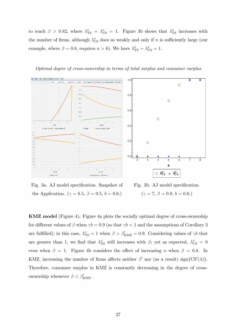
to reach � > 0:82, where �oTS = �oCS = 1. Figure 3b shows that �oTS increases with

the number of �rms, although �oCS does so weakly and only if n is su¢ ciently large (our

example, where � = 0:8, requires n > 6). We have �oTS = �oCS = 1.


Fig. 3a. AJ model speci�cation. Snapshot of

the Application. ( = 8:5, � = 0:5, b = 0:6.)

Fig. 3b. AJ model speci�cation.

( = 7, � = 0:8, b = 0:6.)

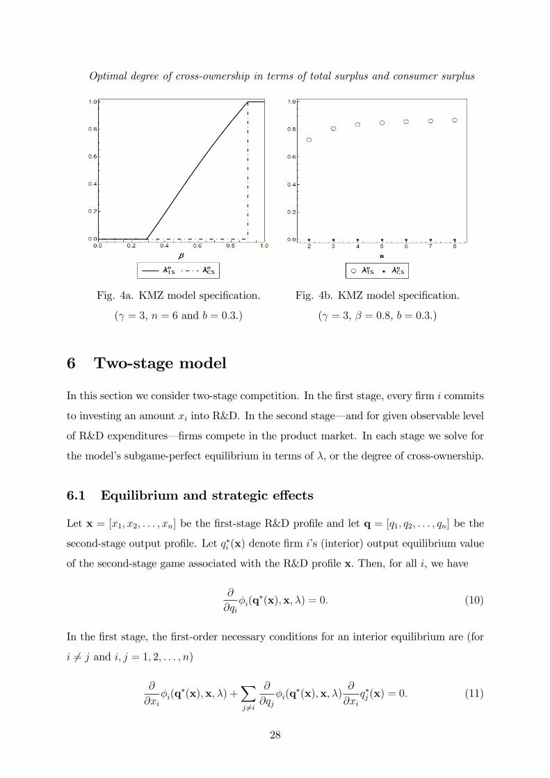
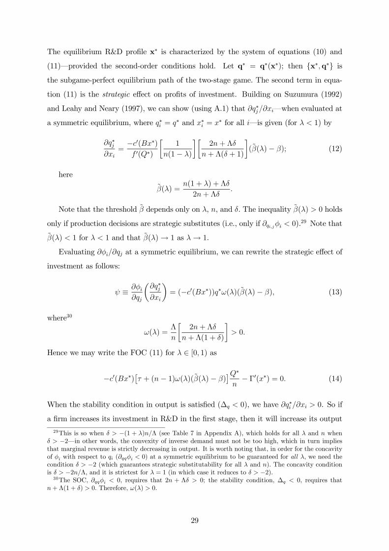
KMZ model (Figure 4). Figure 4a plots the socially optimal degree of cross-ownership

for di¤erent values of � when b = 0:9 (so that b < 1 and the assumptions of Corollary 3

are ful�lled); in this case, �oTS = 1 when � > �0KMZ = 0:9. Considering values of b that

are greater than 1, we �nd that �oTS still increases with �; yet as expected, �oCS = 0

even when � = 1. Figure 4b considers the e¤ect of increasing n when � = 0:8. In

KMZ, increasing the number of �rms a¤ects neither �0 nor (as a result) signfCS0(�)g.

Therefore, consumer surplus in KMZ is constantly decreasing in the degree of cross-

ownership whenever � < �0KMZ.

27


Fig. 4a. KMZ model speci�cation.

( = 3, n = 6 and b = 0:3.)

Fig. 4b. KMZ model speci�cation.

( = 3, � = 0:8, b = 0:3.)

6 Two-stage model

In this section we consider two-stage competition. In the �rst stage, every �rm i commits

to investing an amount xi into R&D. In the second stage� and for given observable level

of R&D expenditures� �rms compete in the product market. In each stage we solve for

the model�s subgame-perfect equilibrium in terms of �, or the degree of cross-ownership.

6.1 Equilibrium and strategic e¤ects

Let x = [x1; x2; : : : ; xn] be the �rst-stage R&D pro�le and let q = [q1; q2; : : : ; qn] be the

second-stage output pro�le. Let q�i (x) denote �rm i�s (interior) output equilibrium value

of the second-stage game associated with the R&D pro�le x. Then, for all i, we have

@

@qi�i(q

�(x);x; �) = 0: (10)

In the �rst stage, the �rst-order necessary conditions for an interior equilibrium are (for

i 6= j and i; j = 1; 2; : : : ; n)

@

@xi�i(q

�(x);x; �) +Xj 6=i

@

@qj�i(q

�(x);x; �)@

@xiq�j (x) = 0: (11)

28

The equilibrium R&D pro�le x� is characterized by the system of equations (10) and

(11)� provided the second-order conditions hold. Let q� = q�(x�); then fx�;q�g is

the subgame-perfect equilibrium path of the two-stage game. The second term in equa-

tion (11) is the strategic e¤ect on pro�ts of investment. Building on Suzumura (1992)

and Leahy and Neary (1997), we can show (using A.1) that @q�j=@xi� when evaluated at

a symmetric equilibrium, where q�i = q� and x�i = x� for all i� is given (for � < 1) by

@q�j@xi

=�c0(Bx�)f 0(Q�)

�1

n(1� �)

��2n+ ��

n+ �(� + 1)

�(~�(�)� �); (12)

here

~�(�) =n(1 + �) + ��

2n+ ��:

Note that the threshold ~� depends only on �, n, and �. The inequality ~�(�) > 0 holds

only if production decisions are strategic substitutes (i.e., only if @qi;j�i < 0).29 Note that

~�(�) < 1 for � < 1 and that ~�(�)! 1 as �! 1.

Evaluating @�i=@qj at a symmetric equilibrium, we can rewrite the strategic e¤ect of

investment as follows:

� @�i@qj

�@q�j@xi

�= (�c0(Bx�))q�!(�)(~�(�)� �); (13)

where30

!(�) =�

n

�2n+ ��

n+ �(1 + �)

�> 0:

Hence we may write the FOC (11) for � 2 [0; 1) as

�c0(Bx�)�� + (n� 1)!(�)(~�(�)� �)

�Q�n� �0(x�) = 0: (14)

When the stability condition in output is satis�ed (�q < 0), we have @q�i =@xi > 0. So if

a �rm increases its investment in R&D in the �rst stage, then it will increase its output

29This is so when � > �(1 + �)n=� (see Table 7 in Appendix A), which holds for all � and n when� > �2� in other words, the convexity of inverse demand must not be too high, which in turn impliesthat marginal revenue is strictly decreasing in output. It is worth noting that, in order for the concavityof �i with respect to qi (@qq�i < 0) at a symmetric equilibrium to be guaranteed for all �, we need thecondition � > �2 (which guarantees strategic substitutability for all � and n). The concavity conditionis � > �2n=�, and it is strictest for � = 1 (in which case it reduces to � > �2).30The SOC, @qq�i < 0, requires that 2n + �� > 0; the stability condition, �q < 0, requires that

n+ �(1 + �) > 0. Therefore, !(�) > 0.

29

in the second stage. At the same time, by equation (12) we have that

sign

�@q�j@xi

�= signf� � ~�(�)g

and that @q�j=@xi > 0 when quantities are strategic complements (since then ~� < 0). In

the case of strategic substitutes, @q�j=@xi > 0 only if � > ~�(�). When a �rm increases the

amount invested in R&D, it exerts two opposite e¤ects on the output decision of rival

�rms. There is a positive e¤ect because rival �rms become more e¢ cient owing to the

presence of spillovers. Yet there is also a negative e¤ect because the reaction of rivals

to �rm i�s higher quantity is to reduce their own output via competing in the market

for strategic substitutes. If spillover e¤ects are strong enough that � > ~�(�), then the

positive e¤ect outweighs the negative e¤ect; this outcome implies that @q�j=@xi > 0.

We can also conduct comparative statics on the threshold value ~�(�). Under Assump-

tion A.1 and from the expression for ~�, it is straightforward to show the following result.

This lemma highlights the crucial role played by demand curvature.

LEMMA 3 For � < 1; the threshold ~�: decreases (resp. increases) with the number of

�rms if demand is concave (resp. convex); increases with the degree of cross-ownership

(@~�=@� > 0) if � > �2; and increases with the curvature of the inverse demand function �

(i.e., @~�=@� > 0).

Since @�i=@qj < 0, it follows that the sign of the strategic e¤ect is opposite to the

sign of @q�j=@xi; that is,

signf g = �sign�@q�j@xi

�= signf~�(�)� �g:

Thus the strategic e¤ect is positive if production decisions are substitutes and if � is

below the threshold ~�. In this case, there are incentives to overinvest because increasing

investment reduces the rival�s output. Then, as shown by Leahy and Neary (1997, Prop. 1)

for � = 0, equations (10) and (14) together imply that output and R&D are higher in

the two-stage model than in the static model.31 It is intuitive that, if � < ~�, then each

31This result is derived under assumptions yielding a unique equilibrium and such that the two models�respective pro�t functions satisfy the Seade stability condition with respect to R&D� namely, that themarginal pro�t of each �rm with respect to R&D must decrease with a uniform increase in R&D by all�rms.

30

�rm expects a higher �rst-stage investment in R&D to reduce the second-stage output of

rival �rms. The implication is that � (@�i=@qj)(@q�j=@xi) > 0 and so each �rm is led

to increase their �rst-stage R&D investments, which in turn boosts output in the second

stage (@q�i =@xi > 0). Observe that ~�(1) = 1: if there is no RJV (� < 1) then, for high

levels of cross-ownership, the strategic e¤ect is always positive (� < ~�). In contrast, if �

exceeds ~� then the strategic e¤ect is negative; hence both output and R&D are lower in

the two-stage model than in the static model.

6.2 Comparative statics on cross-ownership

Next we analyze how the degree of cross-ownership a¤ects the decisions on output and

R&D that are made in equilibrium. By using (13) and by totally di¤erentiating the system

formed by (10) and (11) before evaluating it at a symmetric equilibrium, we can solve

both for @q�=@� and for @x�=@� under regularity conditions. Let s(�) = !(�)�~�(�)� �

�.

We obtain the following result.

LEMMA 4 In the two-stage model :

sign

�@x�

@�

�= sign

�(� + s0(�))P 0(c)�1n� [� + (n� 1)s(�)]

; (15)

sign

�@q�

@�

�= sign

�(� + s0(�))B � �H(�)

: (16)

Moreover, if @x�=@� � 0 then @q�=@� < 0.

So once again we �nd that allowing for some additional degree of cross-ownership

will increase output only if it also boosts R&D. In particular, from (15) we obtain that

@x�=@� > 0 if and only if � > �2S (see the proof of this lemma for more on �2S).

We are now in a position to derive the threshold values of spillovers that determine the

sign of the e¤ect, at equilibrium, of � on R&D and output. In this we assume that there

is a unique positive �, denoted �2S0, that solves the equation (� + s0(�))B = �H(�).32

32To streamline the discussion, here we shall refer simply to the left-hand side (LHS, (� + s0(�))B)and the right-hand side (RHS, �H(�)) of this equation. RHS is a constant in AJ (see Table 3), but itincreases with � in KMZ and CE. Numerical simulations show that LHS is also increasing in � and thatit takes a lower value (than RHS) at � = 0. In AJ there exists a unique �2S

0< 1 when n is su¢ ciently

large� or when and b are su¢ ciently low� and � is su¢ ciently large. In KMZ, RHS increases moreslowly than LHS when and b are smaller whereas LHS increases more rapidly for higher values of �.It follows that, for high � and su¢ ciently low and b, there exists a unique �2S

0that is nearly (but still

less than) 1. In CE, RHS increases faster than LHS and there seems to be no solution, in which caseregion RIII does not exist.

31

Then we have @q�=@� � 0 for � 2 [0; �2S0] and @q�=@� > 0 for � 2 (�2S0; 1]. Therefore:

RI (where @x�=@� � 0 and @q�=@� < 0) occurs when � � �2S; RII (where @q�=@� � 0

and @x�=@� > 0) occurs for � 2 (�2S; �2S0]; and RIII (where @q�=@� > 0 and @x�=@� > 0)

occurs when � > �2S0.

These results extend Proposition 1 to the two-stage model. A direct application of

(15) and (16) allows us to derive the threshold values for each of the model speci�cations

considered in the paper (see Appendix B.2).

Our �ndings are comparable to those of Leahy and Neary (1997, Prop. 3). Those

authors show that if cooperation does not extend to output (i.e, with collusion only at

the R&D level) then the result is reduced output and R&D� unless spillovers are high

enough, in which case �rms increase both output and R&D. These two results correspond

to regions RI and RIII, respectively. In addition, we identify region RII: where cooperation

driven by minority shareholdings leads to less output and more R&D. Another di¤erence

is that, in Leahy and Neary�s model, the spillover threshold above which cooperation

leads to more output and R&D lies strictly between 0 and 1. In contrast, here (as in

the simultaneous choice case) there is no guarantee that RIII exists; that is, �2S0 may lie

above 1.

In the proof of Lemma 7 (see Appendix A) we show that, in the two-stage model,

W 0(�) =

�� f 0(Q�)@q

�

@�

��(1� �)� � !(�)(~�(�)� �)

�(n� 1)c0(Bx�)@x

�

@�

�Q�:

Hence the strategic e¤ect of investment, !(�)(~�(�) � �), plays an important role in de-

termining the impact of cross-ownership on welfare. When the strategic e¤ect is negative

(� > ~�(�)), the two-stage model behaves like the simultaneous model: W 0(�) < 0 in RI,

W 0(�) > 0 in RIII, and W 0(�) either positive or negative (depending on the extent of

spillovers) in RII. Yet when the strategic e¤ect is positive and spillovers are su¢ ciently

low (though not necessarily close to zero), W 0(�) < 0 in RII and W 0(�) can be positive

or negative in RI and in RIII. A consequence of some interest is that, in RIII� where

@x�=@� > 0 and @q�=@� > 0, so consumer surplus increases with � (indeed, � = 1 is

32

optimal for consumers)� total surplus can be decreasing in � for su¢ ciently high �.33

Then, in stark contrast to the simultaneous model and owing to the strategic e¤ect of

investment, for some spillover values it may be that �oCS = 1 > �oTS > 0. We illustrate

this case under the AJ and KMZ model speci�cations in the simulations that follow (see

Figure 6a and Figure 7).34 Similarly as in the simultaneous case, there is a threshold

value ��2S for which �oTS > 0 if � > ��2S; the condition under which ��2S < 1 is given by

Lemma 7 (in Appendix A). If the condition holds thenW 0(0)j�=1 > 0, in which case there

exists a su¢ ciently large spillover value for which some degree of cross-ownership is wel-

fare enhancing. (In Appendix B.2 we derive ��2S for the model speci�cations considered

in this paper.)

6.3 Simulations

This section presents our simulations of the three considered models.35 These simulations

con�rm the qualitative results obtained in the static model, but with two caveats: (i) in

the two-stage model, the socially optimal level of cross-ownership tends to be higher

when spillovers are high; and (ii) in some cases the consumer surplus standard may

call for more cooperation than does the total surplus standard (i.e., �oCS > �oTS > 0).

Result (i) indicates that the strictness of antitrust policy (in terms of limiting cross-

ownership) should be moderated in the two-stage model when spillovers are high. The

reason underlying both results is the strategic e¤ect. When � is high, the strategic e¤ect

is negative and so there are incentives to underinvest; then it pays to increase � in order

to stimulate investment and output (result (i)). We have already observed that result (ii)

may obtain when the strategic e¤ect is positive (which happens for intermediate levels of �

when � is large, since ~�(�)! 1 as �! 1 and so ~�(�) > �); the resulting overinvestment

increases output (and is good for consumer surplus) but comes at the cost of reducing

�rms�pro�ts, reducing total surplus, and �overshooting�marginal cost reductions.

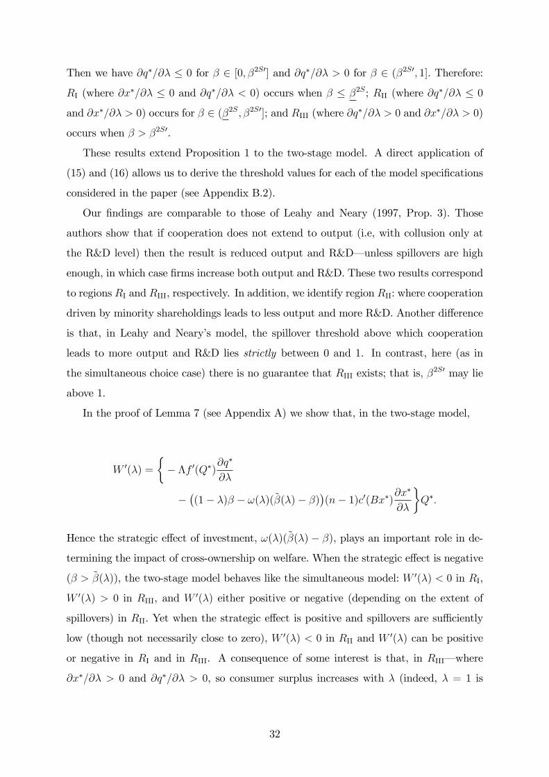
Constant elasticity model. As in the simultaneous case, we observe here that if n

is small then the equilibrium is in RI, which implies that no cross-ownership is socially

optimal. Yet as � and n increase, �oTS also increases. This result is consistent with the

33For � < 1, we have (1� �)� � !(�)(~�(�)� �)j�=1 = �(1� �) < 0.34In CE, as in the simultaneous model, ��CS is usually zero or very close to zero.35Appendix B provides complementary results, explanations, and �gures.

33

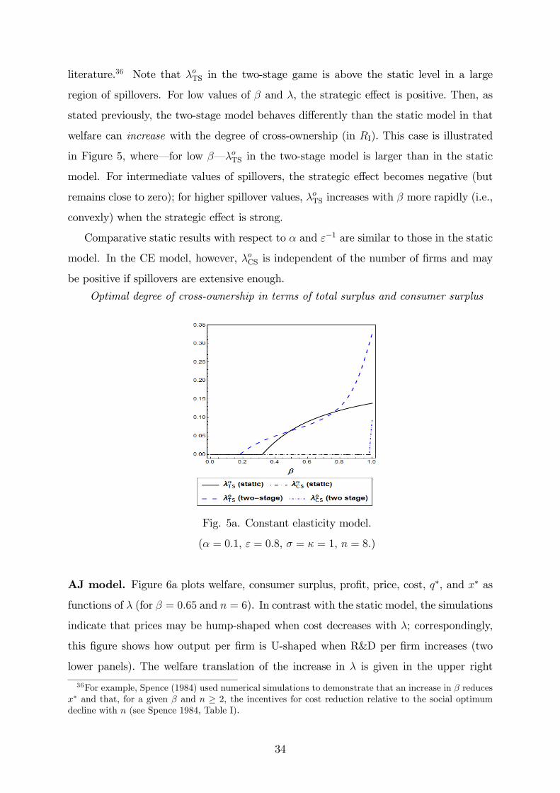
literature.36 Note that �oTS in the two-stage game is above the static level in a large

region of spillovers. For low values of � and �, the strategic e¤ect is positive. Then, as

stated previously, the two-stage model behaves di¤erently than the static model in that

welfare can increase with the degree of cross-ownership (in RI). This case is illustrated

in Figure 5, where� for low �� oTS in the two-stage model is larger than in the static

model. For intermediate values of spillovers, the strategic e¤ect becomes negative (but

remains close to zero); for higher spillover values, �oTS increases with � more rapidly (i.e.,

convexly) when the strategic e¤ect is strong.

Comparative static results with respect to � and "�1 are similar to those in the static

model. In the CE model, however, �oCS is independent of the number of �rms and may

be positive if spillovers are extensive enough.


Fig. 5a. Constant elasticity model.

(� = 0:1, " = 0:8, � = � = 1, n = 8.)

AJ model. Figure 6a plots welfare, consumer surplus, pro�t, price, cost, q�, and x� as

functions of � (for � = 0:65 and n = 6). In contrast with the static model, the simulations

indicate that prices may be hump-shaped when cost decreases with �; correspondingly,

this �gure shows how output per �rm is U-shaped when R&D per �rm increases (two

lower panels). The welfare translation of the increase in � is given in the upper right

36For example, Spence (1984) used numerical simulations to demonstrate that an increase in � reducesx� and that, for a given � and n � 2, the incentives for cost reduction relative to the social optimumdecline with n (see Spence 1984, Table I).

34

panel; it shows U-shaped consumer surplus and increasing pro�t per �rm, with the result

of an interior solution for welfare that features a large value of �oTS > 0. The upper

left panel shows how, for an intermediate range of spillovers, �oCS = 1 > �oTS > 0. This

relation is corroborated in Figure 6b, which also con�rms that in the two-stage model it

is socially desirable to induce more cooperation under the TS standard and also under

the CS standard.


Fig. 6a. AJ model speci�cation. Snapshot of

the Application. (a = 700, c = 500, = 7,

n = 6 and b = 0:6.)

Fig 6b. AJ model speci�cation.

(a = 700, c = 500, = 7, n = 6 and

b = 0:6.)

Satisfying the expression �oCS = 1 > �oTS > 0 becomes possible when the strategic

e¤ect is positive and strong enough. Then there is overinvestment in R&D during the

�rst stage, which boosts output in the second stage. The strategic e¤ect becomes positive

for intermediate values of � when � is a su¢ ciently high. For an intermediate level of

spillovers, total surplus is not maximized with full cooperation because that would entail

too much production (reducing �rms�pro�ts). In Figure 6a we see that output increases

with increasing � and also how fast R&D per �rm increases with �. Only when the

35

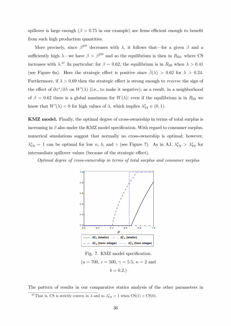
spillover is large enough (� > 0:75 in our example) are �rms e¢ cient enough to bene�t

from such high production quantities.

More precisely, since �2S0 decreases with �, it follows that� for a given � and a

su¢ ciently high �� we have � > �2S0 and so the equilibrium is then in RIII, where CS

increases with �.37 In particular: for � = 0:62, the equilibrium is in RIII when � > 0:41

(see Figure 6a). Here the strategic e¤ect is positive since ~�(�) > 0:62 for � > 0:24.

Furthermore, if � > 0:69 then the strategic e¤ect is strong enough to reverse the sign of

the e¤ect of @x�=@� on W 0(�) (i.e., to make it negative); as a result, in a neighborhood

of � = 0:62 there is a global maximum for W (�): even if the equilibrium is in RIII we

know that W 0(�) < 0 for high values of �, which implies �oTS 2 (0; 1).

KMZ model. Finally, the optimal degree of cross-ownership in terms of total surplus is

increasing in � also under the KMZmodel speci�cation. With regard to consumer surplus,

numerical simulations suggest that normally no cross-ownership is optimal; however,

�oCS = 1 can be optimal for low n, b, and (see Figure 7). As in AJ, �oCS > �oTS for

intermediate spillover values (because of the strategic e¤ect).


Fig. 7. KMZ model speci�cation.

(a = 700, c = 500, = 5:5, n = 2 and

b = 0:2.)

The pattern of results in our comparative statics analysis of the other parameters in

37That is, CS is strictly convex in � and so ��CS = 1 when CS(1) > CS(0).

36

AJ, KMZ, and CE is similar to that for the one-stage game (see Table 5). The only

exceptions we have found are as follow. In AJ: although decreasing b enlarges the region

where �oCS = 1 is optimal (as in the static case), �oCS can be lower than 1 (for a su¢ ciently

low b) when spillovers are su¢ ciently high. In KMZ: although �oCS is independent of n in

the static case, in the two-stage game it can decrease with n when there are few �rms in

the market.

7 Alternative interpretation: R&D cooperation ex-

tending to the product market

The �sympathy coe¢ cient�� can be viewed also as a measure of the intensity of com-

petition; for example, a low � may be the result of �rms� limited scope for collusion

owing to a low discount factor. Note that this parameter has an empirical counterpart

in the estimation of market power because it corresponds to a constant elasticity of con-

jectural variation, which can be used to estimate the degree of industry cooperation.38

Intermediate degrees of cooperation may arise from the strictness of antitrust policy: in

terms of limiting not only cross-shareholdings but also collusion in the product market.

The latter scenario is relevant given the long-standing suspicion that R&D cooperation

facilitates coordination in the product market. This outcome may re�ect the existence

of ancillary restraints (or of other channels through which cooperative R&D may lead to

coordination in the product market)39 or the existence of multimarket contacts.40 There

is also growing evidence that R&D cooperation facilitates product market cooperation

from empirical studies (Duso et al. 2010; Goeree and Helland 2010), from experiments

38Michel (2016) estimates the degree of pro�t internalization after ownership changes in di¤erentiatedproduct industries. He allows each �rm�s objective function to depend on other �rms�pro�ts by incor-porating the parameter �ij , which is the extent to which brand i accounts for brand j�s pro�ts whensetting the optimal brand-i price.39As when, for example, an RJV stipulates downstream market division for any patents that may

result from the venture or when there are collateral agreements that impose cross-licensing of old patents(or a per-unit output royalty for using new patents)� since these circumstances reduce the incentivesof �rms to increase their output (Grossman and Shapiro 1986; Brodley 1990). The various channelsthrough which cooperative R&D may facilitate coordination in the product market are analyzed byMartin (1995), van Wegberg (1995), Greenlee and Cassiman (1999), Cabral (2000), Lambertini et al.(2002), and Miyagiwa (2009). Rey and Tirole (2013) examine how both independent marketing and jointmarketing alliances (e.g., patent pools) can lead to tacit collusion.40See the related evidence in Parker and Röller (1997) for mobile telephony and in Vonortas (2000)

for US RJVs.

37

(Suetens 2008),41 and from antitrust cases.42

Our analysis therefore extends the traditional framework in two directions: no sep-

aration between coordination in R&D and output, whether because of cross-ownership

or because R&D cooperation naturally extends to product market cooperation; and the

presence of intermediate degrees of cooperation in response to the strictness of competi-

tion policy. Antitrust authorities a¤ect the parameter � by limiting cross-shareholdings;

we can also interpret � as a measure of the intensity with which collusion is scrutinized.43

From a policy perspective, our results highlight the tension between a CS standard as

proclaimed by many competition authorities and the fact that R&D cooperation is widely

allowed (and even encouraged) by those same public authorities. Whenever cooperation

in R&D extends to competition in the product market, policy must in general be much

stricter if the aim is to increase consumer surplus.

8 Concluding remarks

In the context of a general symmetric oligopoly Cournot model with cost-reducing R&D

investment, spillovers, and symmetric partial ownership interests, we have identi�ed tight

conditions� in terms of the curvature of demand, market concentration, and the extent

of spillovers� under which cross-ownership is welfare enchancing. We also �nd that the

socially optimal degree of cross-ownership is positively associated with the number of

�rms, with the elasticity of demand and of the innovation function, and with the extent

of spillovers. Yet if the objective is to maximize consumer surplus then (i) the scope for

partial ownership interests is greatly reduced and (ii) �rm entry need not induce, at the

welfare optimum, a higher degree of cross-ownership. We say that an antitrust policy

is strict to the extent that it limits minority shareholdings, and (alternatively) when it

is increasingly activated as cooperation in R&D extends to cooperation in output. The

41Suetens (2008) uses a two-stage duopoloy model to con�rm that cooperation in reducing R&Dcosts facilitates price collusion. Agents engage in cooperative R&D projects more than once, and theyinteract repeatedly in the product market. For both small and large spillovers this author �nds thatcooperativeness in the pricing stage is generally higher when subjects can make binding R&D agreementsthan in the baseline treatments without the possibility of such agreements.42Goeree and Helland (2010) gather a number of cases in the petroleum industry, the computer indus-

try, the market for semiconductor memory, and the telecommunications sector.43Besanko and Spulber (1989) show that, if collusive behavior is unobservable and if production costs

are private information, then the antitrust authority may optimally induce some intermediate degree ofcollusion among �rms.

38

competition-reducing e¤ect of cross-ownership justi�es policy intervention, as forcefully

underscored by the empirical work of Azar et al. (2015, 2016). However, some degree

of cross-ownership may actually be welfare enhancing, and may even increase consumer

surplus, for an industry that exhibits su¢ ciently large R&D spillovers. In the extreme, it

may be socially optimal to form a cartelized RJV when the curvature of the innovation

function is not too large. This paper stipulates precise conditions that can be checked to

see� in industries with signi�cant R&D spillovers� whether cross-ownership is (or is not)

still improving social welfare.

We extend the �simultaneous action�(static) model of R&D investment to a strategic

commitment (two-stage) model and �nd that our results are (with some caveats) robust

to this extension. It turns out that, when spillovers are above a given threshold, �rms

invest less in R&D and produce less in the two-stage than in the static model; hence the

strategic e¤ect of investment becomes negative. In this case, the social gains� from a

higher degree of cross-ownership that induces �rms to invest and approach more nearly

the socially optimal production levels� are even greater. We also characterize how these

gains are a¤ected by the number of �rms, the extent of cross-ownership, and the curvature

of the inverse demand function. Numerical simulations corroborate that, when spillovers

are high, an antitrust policy should be less strict in the two-stage model than in the static

model. In this case, it need no longer be true that the consumer surplus standard calls for

reduced cross-ownership: cooperation may be needed to induce the investment required

for high output, despite that level of investment possibly being excessive from the total

surplus standpoint.

9 Appendix A

9.1 Minority shareholdings

9.1.1 Common-ownership

Letting �ij be the ownership share of �rm j owned by owner/investor i, the total (portfo-

lio) pro�t of owner i is: �i =P

k �ik�k, where �k are the pro�ts of portfolio �rm k. Since

each �rm takes into account its shareholders�incentives through the control weights � ij,

�rm j maximizes a weighted average of its shareholders�portfolio pro�ts:

39

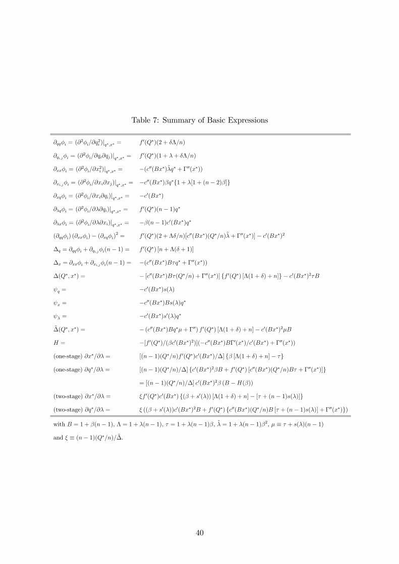
Table 7: Summary of Basic Expressions

@qq�i = (@2�i=@q2i )jq�;x� = f 0(Q�)(2 + ��=n)

@qi;j�i = (@2�i=@qi@qj)jq�;x� = f 0(Q�)(1 + �+ ��=n)

@xx�i = (@2�i=@x2i )jq�;x� = �(c00(Bx�)~�q� + �00(x�))

@xi;j�i = (@2�i=@xi@xj)jq�;x� = �c00(Bx�)�q�f1 + �[1 + (n� 2)�]g

@xq�i = (@2�i=@xi@qi)jq�;x� = �c0(Bx�)

@�q�i = (@2�i=@�@qi)jq�;x� = f 0(Q�)(n� 1)q�

@�x�i = (@2�i=@�@xi)jq�;x� = ��(n� 1)c0(Bx�)q�

(@qq�i) (@xx�i)� (@xq�i)2 = f 0(Q�)(2 + ��=n)[c00(Bx�)(Q�=n)~�+ �00(x�)]� c0(Bx�)2

�q = @qq�i + @qi;j�i(n� 1) = f 0(Q�) [n+ �(� + 1)]

�x = @xx�i + @xi;j�i(n� 1) = �(c00(Bx�)B�q� + �00(x�))

�(Q�; x�) = � [c00(Bx�)B�(Q�=n) + �00(x�)] ff 0(Q�) [�(1 + �) + n]g � c0(Bx�)2�B

q = �c0(Bx�)s(�)

x = �c00(Bx�)Bs(�)q�

� = �c0(Bx�)s0(�)q�

~�(Q�; x�) = � (c00(Bx�)Bq��+ �00) f 0(Q�) [�(1 + �) + n]� c0(Bx�)2�B

H = �[f 0(Q�)=(�c0(Bx�)2)](�c00(Bx�)B�0(x�)=c0(Bx�) + �00(x�))

(one-stage) @x�=@� = [(n� 1)(Q�=n)f 0(Q�)c0(Bx�)=�] f� [�(1 + �) + n]� �g

(one-stage) @q�=@� = [(n� 1)(Q�=n)=�] fc0(Bx�)2�B + f 0(Q�) [c00(Bx�)(Q�=n)B� + �00(x�)]g

= [(n� 1)(Q�=n)=�] c0(Bx�)2� (B �H(�))

(two-stage) @x�=@� = �f 0(Q�)c0(Bx�) f(� + s0(�)) [�(1 + �) + n]� [� + (n� 1)s(�)]g

(two-stage) @q�=@� = � ((� + s0(�))c0(Bx�)2B + f 0(Q�) fc00(Bx�)(Q�=n)B [� + (n� 1)s(�)] + �00(x�)g)

with B = 1 + �(n� 1), � = 1 + �(n� 1), � = 1 + �(n� 1)�, ~� = 1 + �(n� 1)�2, � � � + s(�)(n� 1)

and � � (n� 1)(Q�=n)= ~�.

40

nXi=1

� ij�i =

nXi=1

� ij

nXk=1

�ik�k:

A variety of governance structures may be considered by assigning di¤erent values to the

control rights. Note that the above expression is equivalent to

nXi=1

� ij�ij�j +

nXi=1

� ij

nXk 6=j

�ik�k;

and dividing byPn

i=1 � ij�ij we obtain �j +Pn

i=1 � ijPn

k 6=j �ik�k=Pn

i=1 � ij�ij, or, equiva-

lently,

�j +

nXk 6=j

Pni=1 � ij�ikPni=1 � ij�ij

�k:

Thus, the model of common-ownership with control weights can be re-written in the form

of maximizing �j = �j +Pn

k 6=j �jk�k, where �jk �Pn

i=1 � ij�ik=Pn

i=1 � ij�ij.

9.1.2 Cross-ownership by �rms

The pro�t of �rm j is given by �j = �j+P

k 6=j �jk�k, where �jk is the �rm j�s ownership

stake in �rm k. One can derive the pro�t for each �rm by denoting � = (�1; :::; �n)0 and

� = (�1; :::; �n)0, and solving the equation: � = � +A�, where A is the n � n matrix

with the ownership stakes with 0�s in the diagonal and �jk o¤-diagonal. Thus, � = ��,

where � = (I �A)�1 is the inverse of the Leontief matrix; its coe¢ cients �jk represent

the e¤ective or imputed stake in �rm k�s pro�ts received by a "real" equity holder with

a 1% direct stake in �rm j.44 We examine the symmetric case: �jk = �kj = � for all

j 6= k, and �jj = 0 for all j. The general formula for the coe¢ cients of matrix � when

stakes are symmetric is, for � < 1=(n � 1), �jj = 1�(n�2)�[1�(n�1)�](�+1) and �jk =

�[1�(n�1)�](�+1)

for all j and all j 6= k (see Lemma 8 in Appendix B.1).

Hence, the pro�t of �rm j with symmetric stakes is given by

�j =1� (n� 2)�

[1� (n� 1)�] (�+ 1)�j +�

[1� (n� 1)�] (�+ 1)Xk 6=j

�k:

Maximizing the above expression is equivalent to maximizing �j + �P

k 6=j �k, where

44Gilo et al. (2006, Lemma 1, p.85) also show that �jj � 1 for all j, and 0 � �jk < �jj for all j andall k 6= j.

41

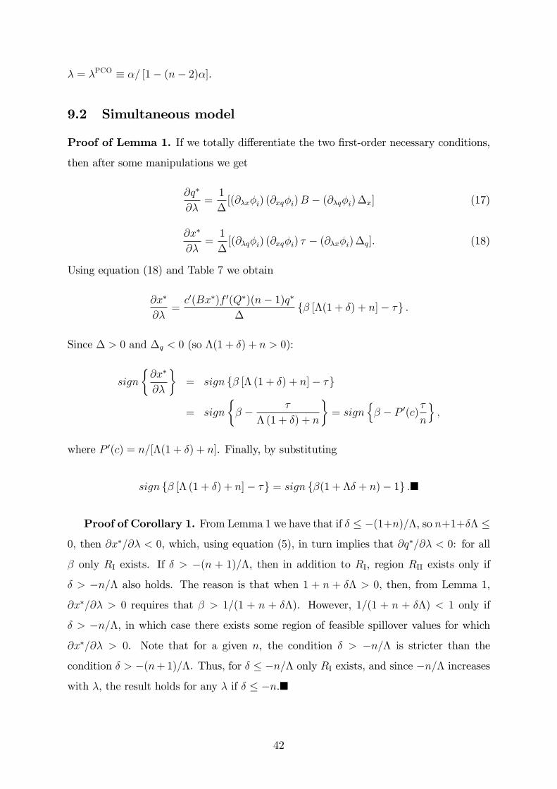
� = �PCO � �= [1� (n� 2)�].

9.2 Simultaneous model

Proof of Lemma 1. If we totally di¤erentiate the two �rst-order necessary conditions,

then after some manipulations we get

@q�

@�=1

�[(@�x�i) (@xq�i)B � (@�q�i)�x] (17)

@x�

@�=1

�[(@�q�i) (@xq�i) � � (@�x�i)�q]: (18)

Using equation (18) and Table 7 we obtain

@x�

@�=c0(Bx�)f 0(Q�)(n� 1)q�

�f� [�(1 + �) + n]� �g :

Since � > 0 and �q < 0 (so �(1 + �) + n > 0):

sign

�@x�

@�

�= sign f� [� (1 + �) + n]� �g

= sign

��

� (1 + �) + n

�= sign

n� � P 0(c)

�

n

o;

where P 0(c) = n=[�(1 + �) + n]. Finally, by substituting

sign f� [� (1 + �) + n]� �g = sign f�(1 + �� + n)� 1g :�

Proof of Corollary 1. From Lemma 1 we have that if � � �(1+n)=�, so n+1+��

0, then @x�=@� < 0, which, using equation (5), in turn implies that @q�=@� < 0: for all

� only RI exists. If � > �(n + 1)=�, then in addition to RI, region RII exists only if

� > �n=� also holds. The reason is that when 1 + n + �� > 0, then, from Lemma 1,

@x�=@� > 0 requires that � > 1=(1 + n + ��). However, 1=(1 + n + ��) < 1 only if

� > �n=�, in which case there exists some region of feasible spillover values for which

@x�=@� > 0. Note that for a given n, the condition � > �n=� is stricter than the

condition � > �(n+1)=�. Thus, for � � �n=� only RI exists, and since �n=� increases

with �, the result holds for any � if � � �n.�

42

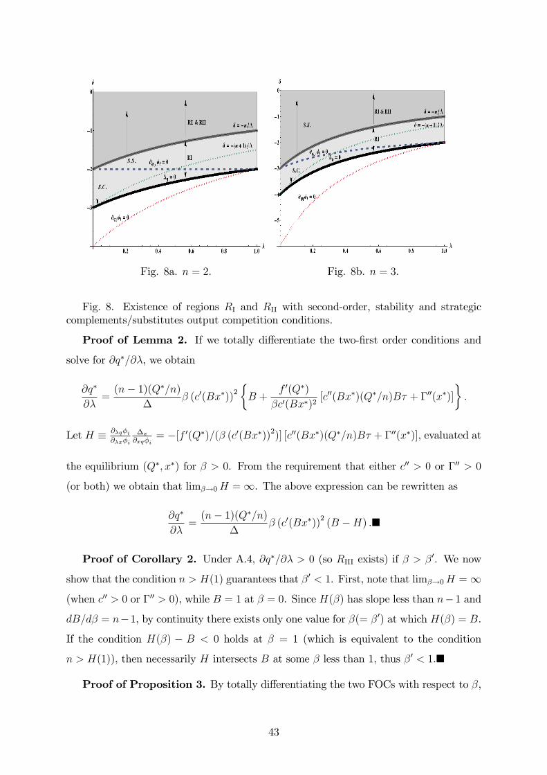
Fig. 8a. n = 2. Fig. 8b. n = 3.

Fig. 8. Existence of regions RI and RII with second-order, stability and strategiccomplements/substitutes output competition conditions.

Proof of Lemma 2. If we totally di¤erentiate the two-�rst order conditions and

solve for @q�=@�, we obtain

@q�

@�=(n� 1)(Q�=n)

�� (c0(Bx�))

2

�B +

f 0(Q�)

�c0(Bx�)2[c00(Bx�)(Q�=n)B� + �00(x�)]

�:

Let H � @�q�i@�x�i

�x@xq�i

= �[f 0(Q�)=(� (c0(Bx�))2)] [c00(Bx�)(Q�=n)B� + �00(x�)], evaluated at

the equilibrium (Q�; x�) for � > 0. From the requirement that either c00 > 0 or �00 > 0

(or both) we obtain that lim�!0H =1. The above expression can be rewritten as

@q�

@�=(n� 1)(Q�=n)

�� (c0(Bx�))

2(B �H) :�

Proof of Corollary 2. Under A.4, @q�=@� > 0 (so RIII exists) if � > �0. We now

show that the condition n > H(1) guarantees that �0 < 1. First, note that lim�!0H =1

(when c00 > 0 or �00 > 0), while B = 1 at � = 0. Since H(�) has slope less than n� 1 and

dB=d� = n�1, by continuity there exists only one value for �(= �0) at which H(�) = B.

If the condition H(�) � B < 0 holds at � = 1 (which is equivalent to the condition

n > H(1)), then necessarily H intersects B at some � less than 1, thus �0 < 1.�

Proof of Proposition 3. By totally di¤erentiating the two FOCs with respect to �,

43

we obtain@q�

@�=1

�[(@�x�i) (@xq�i)B � (@�q�i)�x] (19)

@x�

@�=1

�[(@�q�i) (@xq�i) � � (@�x�i)�q]: (20)

Since @xq�i > 0 and @�q�i > 0, � > 0; �x < 0 and �q < 0, the sign of the impact of �

on output and R&D in equilibrium depends on the sign of @�x�i. It can be shown that

@�x�i = �c0(Bx�)(n� 1)q�

B�

��B

�� (Bx�)

�(21)

and the result follows.�

Proof of Proposition 4. To prove Proposition 4 a few preliminary lemmata (as-

suming A.1-A.4) are useful.

LEMMA 5 Suppose that � > �n, then W 0(�) > 0 if � > �̂ (�) where �̂ is the unique

positive solution to the equation

H(�)�B = [(n� �)=�] [(n+ 1 + ��)� � 1]. (22)

Proof. We �rst derive the condition that determines the spillover threshold value �̂

above which welfare is increasing in the degree of cross-ownership. By inserting @q�=@�

and @x�=@� (given in Table 7) into (8) we obtain:

W 0(�) = ��f 0(Q�)(n� 1)q�

�c0(Bx�)2�(B �H(�))Q�

�(1� �)�(n� 1)c0(Bx�)(n� 1)q�

�f 0(Q�)c0(Bx�) f� [�(1 + �) + n]� �gQ�;

which can be rewritten as:

W 0(�) = #w (� (B �H(�)) + (1� �)(n� 1) f� [�(1 + �) + n]� �g) ;

where #w � [(n� 1)q�=�]c0(Bx�)2(�f 0(Q�))�Q� is positive. Note that (1� �)(n� 1) =

n� �, thus for � > 0, W 0(�) > 0 if

H(�)�B <n� ��

[(n+ 1 + ��)� � 1] : (23)

44

Note that lim�!0H =1 and (by Assumption A.4) the left-hand side of (23) is decreasing

in �. The right-hand side of (23) is increasing in � (since n+ 1+ �� > 0 holds when RII

and RIII exist) and �nite at � = 0. Thus, there exists a unique positive threshold �̂ that

solves the equation (22), and for any � > �̂ condition (23) holds, that is, W 0(�) > 0.�

LEMMA 6 We have that �̂(�) < �0(�) for all �, which implies that �� < �0(0) where

�� = �̂(0). Futhermore, �� < 1 if

n+ (n� 1)(� + n)�H(1) > 0: (24)

Proof. We �rst show that �0(�) > �̂(�) for any �, and as a result �0(0) > �� = �̂(0).

Suppose that for a given �, �̂ > �0, then from (6) we have that for � 2 (�0; �̂) it holds

that @q�=@� > 0. Thus, from equation (5) it also holds that @x�=@� > 0, which implies

from equation (8) that W 0(�) > 0. However, from equation (22) we have that W 0(�) < 0

for � < �̂, a contradiction. Suppose now that �̂ = �0, then we can pick � such that

� = �̂ = �0, and as a result H �Bj�=�0 = 0, thus from equation (22) we have that

�̂ = �0 = 1=(n+1+��), which implies that @x�=@� = 0 (see Table 7), and from equation

(5) this in turn implies that @q�=@� < 0. However, at � = �0, B �H = 0, so @q�=@� = 0

(see Table 7), a contradiction.

The proof of Lemma 5 shows thatW 0(�) > 0 for some � if the spillover is larger than

the threshold value �̂ (�), where �̂ is the unique positive solution to the equation (22).

Furthermore, �̂ < 1 if condition (23) evaluated at � = 1 holds since lim�!0H(�) = 1

and H(�) � B decreases with � (by Assumption A.4), while the right-hand side of (23)

increases with � (for � < 1) and takes �nite value at � = 0. Therefore, by evaluating (23)

also at � = 0 we obtain the condition that ensures that �� < 1, n+(n�1)(�+n)�H(1) >

0.�

We turn now to prove successively each of the statements of Proposition 4.

i) The result follows from Proposition 1: if �� HHI�1, then only RI exists, where

@x�=@� < 0 and @q�=@� < 0, and thus CS 0(�) < 0 and W 0(�) < 0 for all �.

ii) Next we consider the case in which �� < n:

ii.1) �oTS = �oCS = 0 if � � ��. First, we have to show that there does not exist � < ��

such that W 0(�) > 0 for some positive �. However, this follows trivially from

45

the assumption that W (�) is single peaked: since for any � < ��, W 0(0) < 0,

we have that W 0(�) < 0 for all positive �, otherwise there would exist another

stationary point that is a (local) minimum, a contradiction. Similarly, if � = ��,

then W 0(0) = 0, and the assumption that W (�) is single peaked guarantees that

W 0(�) < 0 for any positive �. In addition, if � � ��, then �oCS = 0: from Lemma 6

we know that �0(�) > �� = �̂(0) for all �; since � is assumed to be equal to or lower

than ��, it follows that CS 0(�) < 0 for all �, thus �oCS = 0.

ii.2) �oTS > �oCS = 0 if � 2��; �0 (0)

�. Noting again that �� = �̂(0), the result that

�oTS > 0 when � > �� follows immediately from Lemma 5. In addition, � < �0(0)

yields �oCS = 0: when H is weakly increasing in �, �0(�) also is, and consequently if

� < �0(0), then � < �0(�) for all �, i.e., @q�=@� < 0 for all �, thus �oCS = 0.

ii.3) We �rst show that �oTS > 0 and �oCS > 0 if � > �0 (0). From Lemma 6 it follows

that � > �0(0) > ��, which yields �oTS > 0. From Lemma 2 we know that if for some

given �, � > �0(�), then @q�=@� > 0. Hence if � > �0(0), we have that @q�=@� > 0

at � = 0, which using (9) implies that CS 0(0) > 0, and therefore �oCS > 0

Next we show that �oTS � �oCS when H is weakly increasing in �. Note that B > H

(since @q�=@� > 0) at � = 0. When H is weakly increasing in �, we may face the

following three cases:

� There does not exist some � < 1 at which H = B; as a result @q�=@� > 0 and, by

(5), @x�=@� > 0 for all �, which from equation (8) yields W 0(�) > 0 for all �; thus

�oTS = �oCS = 1.

� There exists an interval subset L of the continuum of values of � in (0; 1] at which

H = B but (a) H never crosses B, so there is no � at which H > B, or (b)

there exists some � above which H > B. In both cases, in the region of values

for � where H = B we have @q�=@� = 0 (or, equivalently, CS 0(�) = 0), while

@x�=@� > 0, consequently W 0(�) > 0. It follows that if H never crosses B or does

it for some � > 1, then �oTS = 1, while any � 2 L is optimal in terms of CS (even

if L is a singleton) since @q�=@� > 0 for any � lower than the lower bound of L,

thus �oTS � �oCS; by the same token, if H > B for some � < 1, then any � 2 L is

optimal in terms of CS (even if L is a singleton), while �oTS is larger or equal than

the upper bound of L, thus �oTS � �oCS.

46

iii) In ii.1) �oTS = �oCS = 0, in ii.2) �oTS > �oCS = 0, and in ii.3) �oTS � �oCS > 0.

Therefore, in the three cases �oTS � �oCS.

For the sake of completeness, next we consider the particular case where � = �0(0).

� Case � = �0(0). If H (as a function of �) is increasing at some value of �, then �0

also is. Thus, for any larger value of �, � < �0(�), which implies that @q�=@� < 0;

as a result, any smaller value of �, where � = �0, and therefore @q�=@� = 0, is

optimal in terms of consumer surplus. Similarly, when H (and therefore �0) is

independent of � for all �, we have that @q�=@� = 0 for all � since � = �0. Hence

CS is independent of �, and any � is optimal in terms of CS. In both cases, for

all � where H = B we have @x�=@� > 0, since @q�=@� = 0, which implies that

W 0(�) > 0. Therefore, �oTS � �oCS � 0.�

9.3 Two-stage model

Proof of Lemma 4. Using (13), by totally di¤erentiating the system formed by (10;

11) in a symmetric equilibrium, and solving for @q�=@� and @x�=@�, we obtain

@q�

@�=1~�f[@�x�i + (n� 1) �] (@xq�i)B � @�q�i [�x + x(n� 1)]g (25)

@x�

@�=1~�

�@�q�i

�@xq�i� + (n� 1) q

�� [@�x�i + (n� 1) �] �q

; (26)

where z � @ =@z with z = q; x; �, and

~�(Q�; x�) = �q [�x + x(n� 1)]� @xq�i�@xq�i� + q(n� 1)

�B;

which is assumed to be strictly positive.45 By rewriting equation (26) as follows

@x�

@�= �f 0(Q�)c0(Bx�) f(� + s0(�)) [�(1 + �) + n]� [� + (n� 1)s(�)]g ; (27)

where � � (n � 1)(Q�=n)= ~� and s(�) = !(�)(~�(�) � �), we get that sign f@x�=@�g is

given by (15). Let us now turn to the impact of � on output in equilibrium. Equation

45We show in Appendix B.2.2 that ~�(Q�; x�) > 0 is also a necessary condition for having a positiveoutput at equilibrium in AJ.

47

(25) can be rewritten as follows

@q�

@�= �

�(� + s0(�))c0(Bx�)2B + f 0(Q�) fc00(Bx�)(Q�=n)B [� + (n� 1)s(�)] + �00(x�)g

�:

(28)

By inserting the �rst-order necessary condition (11) evaluated at the symmetric equi-

librium into the above expression, after some manipulations we get that sign f@q�=@�g

is given by (16). Finally, note that the �rst-order condition with respect to output is

identical to the one associated to the static case. Therefore, by totally di¤erentiating the

FOC with respect to output and solving for @q�=@�, we obtain again equation (5), which

implies that if @x�=@� � 0, then @q�=@� < 0. From (15), we obtain that @x�=@� > 0 if

and only if

� > �2S � 1� (!0(�)~�(�) + !(�)~�0(�))P 0(c)�1n+ !(�)(n� 1)~�(�)

(1 + n+ ��) + (n� 1)!(�)� P 0(c)�1n!0(�):�

LEMMA 7 Under assumptions A.1.-A.4, in the two-stage model, there is a su¢ ciently

large spillover value (��2S < 1) for which allowing some cross-ownership is socially optimal

(�oTS > 0) if

(1+s0(0))n+(1�s(0))(n�1)((1+s0(0))(1+ �+n)� [1 + (n� 1)s(0)]�H(1) > 0: (29)

Proof. See Appendix B.1.�

48

References

[1] Azar, J., Raina, S., Schmalz, M.C., 2016. Ultimate Ownership and Bank Competi-

tion. Working paper.

[2] Azar, J., Schmalz, M.C., Tecu, I., 2015. Anti-competitive e¤ects of common owner-

ship. Ross School of Business Working Paper. No 1235.

[3] Besanko, D., Spulber, D.F., 1989. Antitrust enforcement under asymmetric informa-

tion. Economic Journal 99: 408-25.

[4] Bloom, N., Schankerman, M., Van Reenen, J., 2013. Identifying technology spillovers

and product market rivalry. Econometrica 81: 1347-1393.

[5] Brander, J.A., Spencer, B.J., 1984. Strategic commitment with R&D: the symmetric

case. Bell Journal of Economics 14: 225-235.

[6] Bresnahan, T.F., Salop, S.C., 1986. Quantifying the competitive e¤ects of production

joint ventures. International Journal of Industrial Organization 4: 155-175.

[7] Brodley, J., 1990. Antitrust law and innovation cooperation. Journal of Economic

Perspectives 4: 97-112.

[8] Cabral, L., 2000. R&D cooperation and product market competition. International

Journal of Industrial Organization 18: 1033-1047.

[9] Dasgupta, P., Stiglitz, J., 1980. Industrial structure and the nature of innovative

activity. Economic Journal 90, 266-93.

[10] d�Aspremont, C., Jacquemin, A., 1988. Cooperative and noncooperative R&D in

duopoly with spillovers. The American Economic Review 78: 1133-1137.

[11] d�Aspremont, C., Jacquemin, A., 1990. Erratum. The American Economic Review

80: 641-642.

[12] Duso, T., Röller L-H., Seldeslachts, J., 2010. Collusion through joint R&D: An

empirical assessment. Tinbergen Institute Discussion Paper. TI 2010-112/1.

[13] Edgeworth, F. Y., 1881, Mathematical Physics: An Essay on the Application of

Mathematics to the Moral Sciencies, (Kegan Paul, London).

49

[14] European Commission [EC], 2013. Commission Sta¤ Working Document: Towards

more e¤ective EU merger control. Brussels, 25.6.2013 SWD(2013) 239 �nal.

[15] European Commission [EC], 2014. White Paper: Towards more e¤ective EU merger

control. Brussels, 9.7.2014. COM(2014) 449 �nal.

[16] Farrell, J., Shapiro, C., 1990. Asset ownership and market structure in oligopoly.

RAND Journal of Economics 21: 275�292.

[17] Flath, D., 1991. When is it rational for �rms to acquire silent interests in rivals?,

International Journal of Industrial Organization, Vol. 9, pp. 573�584.

[18] Giannetti, M., Laeven, L., 2009. Pension Reform, Ownership Structure, and Cor-

porate Governance: Evidence from a Natural Experiment. The Review of Financial

Studies 22: 4091-4127.

[19] Gilbert, R., 2006. Looking for Mr. Schumpeter: Where are we in the competition-

innovation debate?, in Adam B. Ja¤e, Josh Lerner and Scott Stern (eds), Innovation

Policy and the Economy 6: 159-215. The MIT Press.

[20] Gilo D., 2000. The Anticompetitive E¤ect of Passive Investment, Michigan Law

Review 99: 1�47.

[21] Gilo, D., Moshe, Y., Spiegel, Y., 2006. Partial cross ownership and tacit collusion.

RAND Journal of Economics 37: 81-99.

[22] Goeree, M., Helland E., 2010. Do research joint ventures serve a collusive function?.

Working Paper 448, Institute for Empirical Research in Economics, University of

Zurich.

[23] Greenlee, P., Cassiman, B., 1999. Product market objectives and the formation of

research joint ventures. Managerial and Decision Economics 20: 115-130.

[24] Griliches, Z., 1990. Patent Statistics as Economic Indicators: A Survey. Journal of

Economic Literature 28: 1661-1707.

[25] Grossman, M., Shapiro, C., 1986. Research joint ventures: An antitrust analysis.

Journal of Law, Economics, & Organization 2: 315-337.

50

[26] Hartwick, J.M., 1984. Optimal R&D levels when �rm j bene�ts from �rm i�s inventive

activity. Economics Letters 16: 165-170.

[27] He, J.J., Huang, J., 2014. Product market competition in a world of cross ownership:

Evidence from institutional blockholdings. Available at SSRN.

[28] Kamien, M., Muller, E., Zang, I., 1992. Research joint ventures and R&D cartels.

The American Economic Review 82: 1293-1306.

[29] Karle, H., Klein, T.J., Stahl, K., 2011. Ownership and Control in a Competitive

Industry. ZEW Discussion Paper No. 11-071.

[30] Katz, M.L., 1986. An analysis of cooperative research and development. The Rand

Journal of Economics 17: 527-543.

[31] Lambertini, L., Poddar, S., Sasaki, D., 2002. Research joint ventures, product dif-

ferentiation and price collusion. International Journal of Industrial Organization 20:

829-854.

[32] Leahy, D., Neary, P., 1997. Public policy towards R&D in oligopolistic industries.

The American Economic Review 87: 642-662.

[33] Levin, R.C., Reiss, P.C., 1988. Cost-reducing and demand-creating R&D with

spillovers. Rand Journal of Economics 19: 538-556.

[34] Martin, S., 1995. R&D joint ventures and tacit product market collusion. European

Journal of Political Economy 11: 733-741.

[35] Michel, C., 2016. Identi�cation and Estimation of Intra-Firm and Industry Compe-

tition via Ownership Change. Mimeo.

Miyagiwa, K., 2009. Collusion and research joint ventures. The Journal of Industrial

Economics 57: 768-784.

[36] Parker, P. M. and Röller, L.-H., 1997. Collusive conduct in duopolies : Multimar-

ket contact and cross-ownership in the mobile telephone industry. Rand Journal of


[37] Reitman, D., 1994. Partial ownership arrangements and the potential for collusion.

The Journal of Industrial Economics 42: 313�322.

51

[38] Rey, P., Tirole, J., 2013. Cooperation vs. collusion: How essentiality shapes co-

opetition. Mimeo.

[39] Reynolds, R.J., Snapp, B.R., 1986. The Competitive E¤ects of partial equity interests

and joint ventures. International Journal of Industrial Organization 4: 141-153.

[40] Salop, S.C., O�Brien, D.P., 2000. Competitive E¤ects of Partial Ownership: Finan-

cial Interest and Corporate Control. Antitrust Law Journal 67: 559-614.

[41] Spence, M., 1984. Cost reduction, competition and industry performance. Econo-

metrica 52: 101-121.

[42] Suetens, S., 2008. Does R&D cooperation facilitate price collusion? An experiment.

Journal of Economic Behavior & Organization 66: 822-836.

[43] Suzumura, K., 1992. Cooperative and noncooperative R&D in an oligopoly with

spillovers. The American Economic Review 82: 1307-1320.

[44] van Wegberg, M., 1995. Can R&D alliances facilitate the formation of a cartel?

The example of the European IT industry. Research Memorandum 004, Maastricht

University, METEOR.

[45] Vives, X., 1999. Oligopoly Pricing: Old Ideas and New Tools, (MIT Press, Boston).

[46] Vives, X., 2008. Innovation and competitive pressure. The Journal of Industrial


[47] Vonortas, N.S., 2000. Multimarket contact and inter-�rm cooperation in R&D. Jour-

nal of Evolutionary Economics 10: 243-271.

[48] Weyl, E.G., Fabinger, M., 2013. Pass-through as an economic tool: Principles of

incidence under imperfect competition. Journal of Political Economy 121: 528-583.

[49] Wilkinson, L.A., White, J.L., 2007. Private equity: Antitrust concerns with partial

acquisitions. Antitrust 21: 28-34.

[50] Ziss, S., 1994. Strategic R&D with spillovers, collusion and welfare. The Journal of

Industrial Economics 42: 375-393.

52

Cross-ownership, R&D Spillovers, and Antitrust...

Documents

Transcript of Cross-ownership, R&D Spillovers, and Antitrust...