Cropping Systems for Groundwater Security in India: Groundwater Responses to Agricultural Land
204
1 CROPPING SYSTEMS FOR GROUNDWATER SECURITY IN INDIA: GROUNDWATER RESPONSES TO AGRICULTURAL LAND MANAGEMENT By DANIEL R. DOURTE A DISSERTATION PRESENTED TO THE GRADUATE SCHOOL OF THE UNIVERSITY OF FLORIDA IN PARTIAL FULFILLMENT OF THE REQUIREMENTS FOR THE DEGREE OF DOCTOR OF PHILOSOPHY UNIVERSITY OF FLORIDA 2011
Transcript of Cropping Systems for Groundwater Security in India: Groundwater Responses to Agricultural Land

1
CROPPING SYSTEMS FOR GROUNDWATER SECURITY IN INDIA: GROUNDWATER RESPONSES TO AGRICULTURAL LAND MANAGEMENT
By
DANIEL R. DOURTE
A DISSERTATION PRESENTED TO THE GRADUATE SCHOOL OF THE UNIVERSITY OF FLORIDA IN PARTIAL FULFILLMENT
OF THE REQUIREMENTS FOR THE DEGREE OF DOCTOR OF PHILOSOPHY
UNIVERSITY OF FLORIDA
2011

2
© 2011 Daniel R. Dourte

3
ACKNOWLEDGMENTS
I am deeply indebted to my advisor, Dr. Dorota Haman, for her substantial support
and her consistent commitment to my research, education, and professional
development. I am very grateful for the help and wise counsel I have received from
each person on my supervisory committee. I sincerely thank you: Dr. Rafael Muñoz-
Carpena, Dr. Sanjay Shukla, Dr. Jim Jones, Dr. Louis Motz, and Dr. Laila Racevskis.

4
TABLE OF CONTENTS page
ACKNOWLEDGMENTS................................................................................................. 3
LIST OF TABLES........................................................................................................... 7
LIST OF FIGURES ...................................................................................................... 10
LIST OF ABBREVIATIONS .......................................................................................... 13
ABSTRACT.................................................................................................................. 16
CHAPTER
1 PROJECT OVERVIEW, GROUNDWATER MANAGEMENT, AND REASONS FOR GROUNDWATER DEPLETION .................................................................... 18
Introduction to Study Area ..................................................................................... 18
Climate of Wargal ............................................................................................ 19
Groundwater System of Wargal ...................................................................... 19
Goals of the Research ........................................................................................... 22
Hypotheses ..................................................................................................... 23
Objectives ....................................................................................................... 23
Groundwater in India: Evidence for and Causes of Depletion ................................ 24
Wargal Regional Groundwater Monitoring ....................................................... 24
Northwest India Large Region Groundwater Decline ....................................... 24
Groundwater Balance and Agricultural Management ...................................... 25
Historical Data: Rice Cropland Extent, Groundwater Irrigated Area, Rainfall ... 27
Water Balance Simulation Methods and the Soil and Water Assessment Tool ...... 30
Soil and Water Assessment Tool Overview ..................................................... 30
Summary of Water Balance Simulation Methods............................................. 32
Hydrology in Ungauged Basins ....................................................................... 38
Factors Influencing Groundwater Recharge: Literature Review ............................. 39
Rationale and Significance of a Groundwater Recharge Literature Review ..... 39
Land Surface Environmental Factors and Groundwater Recharge .................. 41
Land use and land cover ........................................................................... 43
Topography .............................................................................................. 45
Soil properties ........................................................................................... 47
Quantifying Groundwater Recharge ................................................................ 48
Discussion and Conclusions on Factors Influencing Groundwater Recharge .. 49
Options for Managing Groundwater in Agricultural Systems .................................. 50
Contributions of this Research ............................................................................... 51
2 RAINFALL INTENSITY-DURATION-FREQUENCY RELATIONSHIPS FOR ANDHRA PRADESH, INDIA: CHANGING RAINFALL PATTERNS AND IMPLICATIONS FOR GROUNDWATER RECHARGE .......................................... 63

5
Rainfall Characterization and Water Resource Management ................................. 63
Groundwater Resources in India ........................................................................... 64
Objectives: Precipitation Characterization and Groundwater in India ..................... 65
Rainfall Characterization........................................................................................ 67
Overview of IDF Analysis ................................................................................ 67
Methods for Rainfall IDF Development for Andhra Pradesh ............................ 68
Exploration of Trends in Occurrence of Rainfall Events of High and Low Intensity ....................................................................................................... 70
Results and Discussion: IDF Curves and Event Intensity Trends ........................... 71
Discussion: Precipitation Characterization and Groundwater in India .................... 72
Conclusions on Rainfall Intensity Trends and Groundwater Recharge................... 73
3 IMPORTANCE OF SURFACE STORAGE PONDING DEPTH FOR PREDICTING INFILTRATION AND RUNOFF IN WATER CONSERVATION TILLAGE SYSTEMS .............................................................................................. 79
Modeling Infiltration and Tillage: Implications for Groundwater Recharge .............. 79
Infiltration, Surface Storage, and Changing Precipitation Character ................ 79
Green-Ampt Infiltration and Depression Storage ............................................. 81
Groundwater Recharge and Tillage Management: Modeling Implications ....... 83
Methods for Analyzing the Importance of Surface Storage Depth .......................... 87
Site Description ............................................................................................... 87
Local Sensitivity Analysis ................................................................................ 88
Global Sensitivity Analysis .............................................................................. 88
Parameters for Green-Ampt Infiltration Sensitivity Analysis ............................. 90
Development and Selection of Design Storms for the Analysis ....................... 93
Results and discussion of GAML Infiltration Sensitivity Analyses........................... 93
Representative Design Storm for the Analysis ................................................ 93
Tillage and MDS: GAML solution form ............................................................ 94
Local sensitivity analysis ................................................................................. 95
Global Sensitivity Analysis .............................................................................. 96
Conclusions on the Importance of Surface Storage Depth for Tillage Parameterization ................................................................................................ 97
4 EVALUATION OF AGRICULTURAL MANAGEMENT ALTERNATIVES FOR SUSTAINABLE GROUNDWATER IN INDIA: SIMULATED WATER BALANCE RESULTS ............................................................................................................ 106
Overview of Water Balance Simulation ................................................................ 106
Groundwater Management in India ............................................................... 106
Goals of Simulated Water Balance Experiments ........................................... 108
Water Balance Simulation Methods ..................................................................... 108
SWAT Preparation ........................................................................................ 108
Describing agricultural management ....................................................... 109
SWAT process modifications .................................................................. 110
SWAT Calibration and Evaluation ................................................................. 111
Parameter sensitivity and uncertainty analysis ........................................ 114

6
Reservoir volume .................................................................................... 118
Groundwater recharge ............................................................................ 120
Results: SWAT Calibration, Evaluation, and Parameter Sensitivity ...................... 122
Uncertainty of Model Predictions ................................................................... 123
Groundwater Balance.................................................................................... 123
Results: Evaluation of Management Alternatives for Sustainable Groundwater ... 125
Significance of Tillage and MDS .................................................................... 126
Changing Extent and Irrigation Management of Rice Croplands ................... 128
Alternatives to Rice: Irrigated and Rainfed Crops .......................................... 129
Conclusions on Agricultural Management and Groundwater Supply in India ....... 130
5 SOCIAL AND ECONOMIC ASSESSMENT OF GROUNDWATER MANAGEMENT ................................................................................................... 149
Groundwater and Indian Agricultural Economics ................................................. 149
Fieldwork on the Socioeconomics of Agricultural Management ........................... 150
Sustainability: Definitions .............................................................................. 151
Methods for Learning about Wargal Agricultural Management ...................... 152
Social and Biophysical Analysis Connections ................................................ 154
Results of Household Survey Fieldwork ........................................................ 154
Main concerns ........................................................................................ 155
Changes in groundwater and climate ...................................................... 156
Management and decision making.......................................................... 159
Valuing Groundwater ........................................................................................... 162
Economics of Alternative Agricultural Management ............................................. 163
Discussion and Summary of Fieldwork on the Socioeconomics of Agricultural Management .................................................................................................... 165
6 LIMITATIONS, APPLICATIONS, AND CONCLUSIONS OF THE WARGAL STUDY OF GROUNDWATER DEPLETION AND AGRICULTURAL MANAGMENT ..................................................................................................... 174
Limitations ........................................................................................................... 174
Applications ......................................................................................................... 175
Conclusions ......................................................................................................... 176
APPENDIX
A SWAT CODE MODIFICATIONS .......................................................................... 180
B INTERVIEW QUESTIONS FOR WARGAL FARMERS ........................................ 187
LIST OF REFERENCES ............................................................................................ 189
BIOGRAPHICAL SKETCH ......................................................................................... 204

7
LIST OF TABLES
Table page 1-1 Areas (ha) of cropland for three-crop rotation in Wargal .................................... 58
1-2 Climate and hydrologic monitoring systems: observation numbers, frequency, purpose ............................................................................................................. 60
1-3 Sources and factors included in analysis by Gogu and Dassargues; adapted from Gogu and Dassargues 2000 ...................................................................... 60
1-4 Summary of methods for quantifying groundwater recharge.............................. 61
1-5 Summary of the 9 recharge studies highlighting dominant factors ..................... 62
2-1 Annual maximum series rainfall intensity generated from hourly rainfall data from Hyderabad, Andhra Pradesh, India. Annual and Kharif season (June-September) total rainfall and rain days. ............................................................. 75
2-2 Parameters for Weibull CDF: F(I) = 1 - exp(-(I/α))β, where I is rainfall intensity, and parameters for IDF function: ................ 75
2-3 Rainfall intensity values from Weibull cumulative distribution functions (CDFs): hourly data 1993-2008 for Hyderabad .................................................. 76
2-4 Rainfall intensity (mm/hr) from Kothyari and Garde general formula fitted to recent intensity data (1993-2008) for Hyderabad1. RMSE calculated based on CDF intensities. ............................................................................................ 77
2-5 Rainfall intensity (mm/hr) from Kothyari and Garde original formula fitted to older intensity data (1950-1980) for southern zone of India1. RMSE calculated based on CDF intensities. ................................................................ 77
2-6 Differences (mm/hour) in predicted rainfall intensity values between Kothyari and Garde IDF formula using 1992 parameters1 and using updated parameters fitted from this study2 ...................................................................... 78
3-1 Parameter values needed for Green-Ampt model: minimum, maximum, mean values and estimated probability distributions. Initial water content (θi), saturated water content (θs), effective hydraulic conductivity (Kse), wetting front suction (ψf), and maximum depression storage depth (MDS) for conventional tillage (CT) and tied-ridge tillage (TR). ........................................ 100
3-2 IDF data (1993 – 2008 hourly rainfall), Weibull distribution used, values in the table are rainfall intensities in mm/hour ........................................................... 101

8
3-3 4-hour design storms of 2, 5, 10-year return period used for rainfall input in GAML sensitivity analysis; 20 min time step .................................................... 102
3-4 GAML predicted runoff (RO) and infiltration (F) depths of conventional (CT) and tied-ridge (TR) tillage for 2 year, 4-hour storm; standard and complete GAML solutions. Min, mean, and max MDS were 0, 5, 10 mm for CT and 15, 32.5, 50 mm for TR. ........................................................................................ 102
3-5 First order sensitivity indexes (Si) for output F of the 5 GAML parameters for tied-ridge (TR) and conventional tillage (CT) for both GAML solution forms, complete and standard. ................................................................................... 104
4-1 Descriptions of 25 alternative management scenarios with abbreviations used ................................................................................................................ 135
4-2 Maximum surface area and volume of the six reservoirs (tanks) in Wargal watershed ....................................................................................................... 138
4-3 Specific yield, natural recharge, and total recharge from DWTF method and total recharge from SWAT simulations in 2009 and 2010 ................................ 138
4-4 Nash-Sutcliffe Efficiency (NSE), percent bias (PBIAS), and ratio of the root mean square error to the standard deviation of measured data (RSR) ............ 139
4-5 Parameter name, t-statistic, p-value, and range of the 13 parameters estimated during SWAT calibration ................................................................. 140
4-6 Summary of selected water balance components for existing and alternative agricultural management, sorted by groundwater balance (GW balance = recharge – irrigation). GW ∆h is predicted groundwater level change, mm, given specific yield of 0.013 from DWTF method. Simulations using generated weather 2000-2009, 792 mm rainfall. ............................................. 141
4-7 Summary of selected water balance components for existing and alternative agricultural management, sorted by groundwater balance (GW balance = recharge – irrigation). GW ∆h is predicted groundwater level change, mm, given specific yield of 0.013 from DWTF method. Simulations using observed weather 2009, 667 mm rainfall. ........................................................ 142
4-8 Sensitivity of annual surface runoff and groundwater recharge to MDS at the basin scale: mm change in depth of recharge and runoff (from existing tillage, MDS = 0) per mm MDS ................................................................................... 146
4-9 Sensitivity of annual surface runoff and groundwater recharge in rainfed croplands (corn and cotton) in kharif season to MDS: mm change in depth of recharge and runoff (from existing tillage, MDS = 0) per mm MDS .................. 146

9
5-1 Concerns of community members ranked (for women) in order of decreasing frequency of reporting ..................................................................................... 168
5-2 Ways of observing groundwater depletion ....................................................... 168
5-3 Perceived causes of local groundwater depletion ............................................ 168
5-4 Suggested reasons for recent reductions in local rainfall amounts .................. 169
5-5 Information used to decide about crop selection: ranked (greatest to least – women’s column) percentages of responses ................................................... 169
5-6 Information used to decide about irrigation management: ranked (greatest to least – women’s column) percentages of responses ....................................... 169
5-7 Decision category and associated most important responses ......................... 171
5-8 Percentages of responses concerning who is responsible for irrigation pump control ............................................................................................................. 172
5-9 Percentages of responses concerning who is responsible for purchase farm inputs (seed and fertilizer) ............................................................................... 172
5-10 Literature review of yield increase for selected crops in response to tied-ridge tillage; methods are measured yield (obs) or simulated yield (sim) .................. 172
5-11 Yields of crops commonly grown in Wargal based on household surveys and state agency data. Sample size indicates number of households that responded to surveys about yield data. Value ($/kg) based on 2009-2010 government of India minimum support prices (MSP) ....................................... 173
5-12 Groundwater balances (mm) and estimated values (USD) of the selected top seven management scenarios (Chapter 4) ...................................................... 173

10
LIST OF FIGURES
Figure page 1-1 Study area location in Wargal mandal, eastern Medak district, northwestern
Andhra Pradesh ................................................................................................ 53
1-2 Groundwater system diagram of Wargal (adapted from Dewandel et al., 2006 and Marechal et al., 2006). t is layer thickness, values are approximate. Water table height fluctuates between 15 and 35 m below surface. .................. 54
1-3 Water balance diagram showing connections between unsaturated and saturated zone water balances. I is irrigation, P is precipitation, SS is surface storage, Inf is infiltration, ET is evapotranspiration, RO is runoff, UF is unsaturated flow, CR is capillary rise, R is groundwater recharge, DP is deep percolation, SF is saturated flow. ....................................................................... 55
1-4 Total annual harvested areas of rice in India and Andhra Pradesh, 1961-2001 .................................................................................................................. 56
1-5 Area equipped for mechanized irrigation from groundwater source in India: 1961, 1971, 1981, 1986, 1993; population of India each year from 1961 to 2007. ................................................................................................................. 56
1-6 Annual rainfall in Telangana region (1960 – 2008): slight declining trend observed (about 3 mm/year reduction in annual rainfall if trend is assumed linear) ................................................................................................................ 57
1-7 Annual rainfall trends (1960 – 2008) in the 3-state region of the GRACE study of Rodell et al., 2009 ................................................................................ 57
1-8 Watershed boundary, reservoir locations (large dots), and digital elevation model of Wargal watershed, 2.2 m resolution .................................................... 58
1-9 Variogram plot of % clay in layer 1 of Wargal soil: used to evaluate spatial autocorrelation of soil properties and for kriging to generate continuous map of soil data ......................................................................................................... 59
2-1 Intensity duration frequency curves for 1, 2, 4, 8, and 24 hour durations developed from hourly rainfall data from 1993 – 2008 from Hyderabad, India ... 76
2-2 Annual counts of high (I ≥ 50 mm/day) and light intensity (5 < I < 50 mm/day) rainfall events (1974-2008) ................................................................................ 78
3-1 Illustration of infiltration modeled by Green-Ampt equation. θ, θs, θi, are volumetric water content, saturated and initial, respectively, hp is depth of water ponded at the surface, L is distance from surface to the wetting front, ψf is wetting front suction. .................................................................................. 99

11
3-2 Typical furrowed field beside tied-ridged field following rain event (image from Jones and Baumhardt 2003) ..................................................................... 99
3-3 Empirical CDF for annual maximum series (AMS) rainfall intensity for 4 hour storms; Weibull, Gamma, and Gumbel CDF fitted to AMS data using maximum likelihood parameter estimation. ...................................................... 100
3-4 Infiltration (F) and runoff (RO) for a 4-hour 2 year design storm; complete and standard GAML solutions ................................................................................ 101
3-5 Infiltration and runoff % changes from mean MDS values for 2 year, 4-hour storm for both GAML solution types; min, mean, max are values of MDS for conventional (CT: 0, 5, 10 mm) and tied-ridge (TR: 15, 32.5, 50 mm) tillage. .. 103
3-6 Total effect sensitivity indices (outputs are F and RO; their sensitivities to each parameter are equal) for Green-Ampt parameters for tied-ridge and conventional tillage for 4 hour design storm of 2 year return period. ................ 105
4-1 Observed and simulated (for calibration and validation) watershed outlet reservoir volume and rainfall in Wargal watershed; 3/19/2010 to 12/3/2010 .... 137
4-2 Simulated and observed reservoir volumes: 3/19/2010 to 12/3/2010 ............... 137
4-3 Observed roundwater level change and rainfall during wet and dry periods .... 139
4-4 Basin-scale response of groundwater recharge, groundwater balance, and runoff to MDS changes in rainfed croplands in kharif season and in both kharif and rabi seasons. MDS of 15, 32.5 or 50 mm. 30 to 50% less runoff with tillage for 15 mm < MDS < 50 mm; groundwater balance from -11 mm for existing management to 7 mm for 50 mm MDS in rainfed areas in both seasons. .......................................................................................................... 143
4-5 Field-scale response of groundwater recharge and runoff to tillage changes (MDS depth) in rainfed croplands in kharif season. MDS of 15, 32.5 or 50 mm. 54 to 83% less runoff from rainfed croplands with tillage for 15 mm < MDS < 50 mm; groundwater balance from -11 mm for existing management to 6 mm for 50 mm MDS in rainfed areas in both seasons. ............................. 144
4-6 Field-scale response of groundwater recharge and runoff to tillage changes (MDS depth) in rainfed croplands in both kharif and rabi seasons ................... 145
4-7 Irrigation, recharge, ET, and groundwater balance for tied-ridge tillage scenarios: 3 MDS depths in rainfed areas in kharif, rabi, and both seasons .... 147
4-8 Irrigation, recharge, ET, and groundwater balance for selected changes in extent and irrigation management of rice croplands ........................................ 148

12
5-1 Some women take a break for lunch and to participate in discussions for this research .......................................................................................................... 170
5-2 One of six water harvesting structures (tanks) in the Wargal watershed used for increasing groundwater recharge ............................................................... 171

13
LIST OF ABBREVIATIONS
ANGRAU Acharya N.G. Ranga Agricultural University: located in Hyderabad, India; partner university in this research
AQUASTAT This is the global web-based information system on water resources and agriculture, developed by the Land and Water Division of the United Nations FAO
ARS Agricultural Research Service of the USDA
CDF Cumulative distribution function
CGWB Central Groundwater Board of India: a Ministry of Water Resources organization responsible for monitoring and maintaining sustainable groundwater resources in India
CN Curve Number: an empirically-based parameter used in the prediction of CN runoff and infiltration; developed by the Natural Resources Conservation Service (NRCS, formerly SCS) of the USDA
CSIRO9 Commonwealth Scientific and Industrial Research Organization: climate model
CT Conventional Tillage
DEM Digital Elevation Model: a raster-based representation of topography
DRASTIC A groundwater vulnerability mapping method
ET Evapotranspiration: the combination of plant transpiration and evaporation of water from soil, surface water, and vegetation surfaces
FAO Food and Agriculture Organization of the United Nations
FAOSTAT A database of time-series information on food and agriculture: developed and supported by FAO
GAML Green-Ampt Mein Larson: physically based infiltration equations developed by Green and Ampt (1911) and improved by Mein and Larson (1973)
GEV Generalized Extreme Value: a family of probability distributions that includes the Gumbel, Fréchet and Weibull distributions as special cases

14
GIS Geographic Information System: software tools used in the development and analysis of spatial data
GLUE Generalized Likelihood Uncertainty Estimation: a simple, generic numerical method for use in calibration and uncertainty analyses of models of systems
GRACE Gravity Recovery and Climate Experiment: twin orbiting satellite system used for observations about TWS
GSA Global Sensitivity Analysis
HYETOS A computer program used for stochastic disaggregation of rainfall to shorter time scales
IAHS International Association of Hydrological Sciences
ICRISAT International Crops Research Institute for the Semi-Arid Tropics
IDF Intensity, duration, frequency: relationships describing the rainfall pattern of a certain location
IPCC Intergovernmental Panel on Climate Change
LSA Local Sensitivity Analysis
LULC Land use and land cover: describes the natural and human-made landscapes
MDS Maximum depression storage: the greatest area-averaged depth of water that can be stored on the surface of a land area before runoff occurs
MSP Minimum Support Price: an Indian national agriculture policy that sets the lowest prices for selected crops
NASA National Aeronautics and Space Administration of the United States government; responsible for aerospace research
NSE Nash-Sutcliffe Efficiency: a model evaluation quantity
NSS Near surface storage: depth of water stored in surface depressions, comparable to MDS
PBIAS Percent bias: a model evaluation quantity
PUB Predictions in Ungauged Basins: and IAHS initiative to reduce model prediction uncertainty

15
RSR The ratio of the root mean square error in model predictions to the standard deviation of measured data: a model evaluation quantity
SCS Soil Conservation Service of the USDA; now called the Natural Resources Conservation Service (NRCS)
SINTACS A groundwater vulnerability mapping method adapted from DRASTIC for improved performance in Mediterranean areas
SWAT Soil and Water Assessment Tool: a distributed-parameter, landscape-scale, open-source hydrologic model
TAW Total available water: depth of water in soil that is extractable by plants
TR Tied-Ridge tillage
TWS Terrestrial water storage: total amount of water stored in a specified land area during some time
UKHI United Kingdom Meteorological Office High Resolution General Circulation Model: a global climate model
USDA United States Department of Agriculture
WAVES A biophysically based water balance model

16
Abstract of Dissertation Presented to the Graduate School of the University of Florida in Partial Fulfillment of the Requirements for the Degree of Doctor of Philosophy
CROPPING SYSTEMS FOR GROUNDWATER SECURITY IN INDIA:
GROUNDWATER RESPONSES TO AGRICULTURAL LAND MANAGEMENT
By
Daniel R. Dourte
May 2011
Chair: Dorota Z. Haman Major: Agricultural and Biological Engineering
The total annual groundwater withdrawals in India (251 billion km3) are the highest
of any nation. Depletion of groundwater resources is increasingly common in much of
India, and farmers bear significant costs and greater vulnerability resulting from the loss
or reduction of a reliable irrigation source. Three hypotheses were tested: (1) current
rice cropland extent and management practices are depleting groundwater supplies, (2)
tillage for water harvesting can significantly increase groundwater recharge in rainfed
croplands, and (3) there are combinations of tillage, crop selection, and irrigation that
are likely to increase groundwater recharge and reduce groundwater withdrawals. In
order to test these hypotheses, there was the objective to evaluate improvements to the
Green-Ampt infiltration routines of a hydrologic model, the Soil and Water Assessment
Tool (SWAT), through the addition of a dynamic surface storage depth used for tillage
parameterization. Also, the final objective was to assess the social and economic
impacts of alternative agricultural land management. SWAT was used for simulating
the groundwater balance (recharge – irrigation pumping) of a 512 ha watershed to
examine a variety of possible agricultural management options for groundwater

17
sustainability. The best options for groundwater sustainability were evaluated based on
predictions of groundwater recharge and withdrawals, evapotranspiration, and
estimated household incomes. Reductions in rice cropland areas significantly improved
the groundwater balance of the study area; water harvesting tillage simulated in all
rainfed areas increased groundwater recharge by about 30 mm/year. Surface storage
depth was shown to be the most important parameter for infiltration prediction in
agricultural systems having 1.5 to 5.0 cm of surface storage capacity; surface storage
depth was still important for infiltration prediction in systems having 0 to 1.0 cm of
surface storage capacity. The vast extent of rice cropland areas and their highly
negative groundwater balance suggest that irrigation from groundwater resources has
caused much of the observed groundwater decline in India. Sensitivity analyses
suggest that the addition of a variable surface storage depth head to the Green-Ampt
infiltration routine can reduce uncertainty in infiltration simulations. Evidence of rainfall
characterized by storms of greater intensity suggests that surface storage of runoff will
become increasingly important for maintaining or improving current levels of
groundwater recharge. Estimates of the economic impacts of selected management
scenarios show promise that moderate management changes to improve the
groundwater balance can still maintain or increase total watershed-scale income.

18
CHAPTER 1 PROJECT OVERVIEW, GROUNDWATER MANAGEMENT, AND REASONS FOR
GROUNDWATER DEPLETION
Introduction to Study Area
There is general agreement that water scarcity in India is severe (Alcamo et al.,
2000; Yang et al., 2003). Total (761 km3) and agricultural (688 km3) water withdrawals
for India in are the highest in the world (AQUASTAT, 2010). Groundwater in India is a
highly important resource for irrigation and household use, and its extensive use is
resulting in widespread groundwater depletion (Shah et al., 2003; CGWB, 2007; Rodell
et al., 2009). More than half of the irrigation requirements of India are met from
groundwater (CGWB, 2002; Shah et al., 2003), and the number of mechanized
borewells in India has increased from less than 1 million in 1960 to 26-28 million in 2002
(Mukherji and Shah, 2005).
India is characterized by substantial diversity in climate zones and landscapes.
One of the highest annual rainfall averages occurs in Cherrapunji in northeastern India:
11,430 mm. Western Rajasthan of northwestern India averages only 37 mm of annual
rainfall; the national average annual rainfall is 1083 mm/year. India is the second most
populous and seventh largest country in the world (1.18 billion people, 328 Mha of total
area and 180 Mha agricultural area; FAOSTAT, 2010).
The study area being considered here is in the Wargal mandal (a mandal is a
local organizational unit, similar to a county) of Medak district, Andhra Pradesh, in the
southern, central part of India. This area was selected by Indian collaborators from
Acharya N.G. Ranga Agricultural University (ANGRAU) in Hyderabad, Andhra Pradesh.
Figure 1-1 illustrates the location of the study area. This 512 ha watershed was
selected for analysis because of its relative proximity to ANGRAU and because it is

19
illustrative of the common regional problem of groundwater decline, making farming
systems increasingly vulnerable. There are 157 households with landholdings in
Wargal; 198 borewells are found in Wargal.
Climate of Wargal
The annual average rainfall in Wargal is 780 mm; about 80% of rainfall is received
from June-September from the southwest monsoon system. Average annual Potential
evapotranspiration (PET) in Wargal is between 1600 and 2000 mm/year (UNEP, 1992).
PET is the amount of water that would be evaporated and transpired from a landscape
that had no soil moisture deficit. The year is divided into three seasons: kharif season is
the rainy season and most important growing season from June-September, rabi is the
season from October-February, summer is the very hot, dry season from March-May.
Groundwater System of Wargal
Groundwater in the Wargal study area occurs, based on field observations
(CGWB, 2007) and the work of Marechal et al. (2006), under largely unconfined
conditions in consolidated formations (fractured granite; transmissivity: 100 to 150
m2/day; specific yield: 0.010 to 0.015). The study by Marechal et al. (2006), in a
watershed nearby the Wargal area, characterizes the hydrogeology as being Archean
granite overlain by a clayey-sandy regolith layer. This is consistent with the general
hydrogeological characterization developed by Dewandel et al. (2006) for hard-rock
aquifers in India. The fissured granite layer, 20-35 m thickness, is typically where
borewell casings are screened for groundwater withdrawal; this layer also is responsible
for much of the horizontal flow (Dewandel et al., 2006). The water table is 15-30 m
below the ground surface, and there is very little interaction with surface water. The

20
diagram of Figure 1-2 (adapted from Marechal et al., 2006) describes the aquifer
system of Wargal.
There are sometimes increased water quality problems as groundwater levels
become reduced; this is often to due naturally occurring arsenic and fluoride in the
geology and soils of a region (Khan, 1994, concerning arsenic in Bangladesh; Subba
Rao and Devadas, 2003, concerning fluoride in India). The concentrations of fluoride
and arsenic in groundwater are sometimes greater deeper in an aquifer, and more
water is withdrawn from deeper in the system as water levels decline. There have been
anecdotal reports of some people in Wargal showing mild symptoms of fluoride
contamination (Reddy, 2009), and the study of Subba Rao and Devadas (2003) in a
district in western Andhra Pradesh documents a number of cases of fluoride-
contaminated groundwater.
The Wargal watershed is located in the northwestern Andhra Pradesh district of
Medak; groundwater resources for the Medak district (in 2005) were a total renewable
groundwater volume of 813.19 Mm3 and a net annual draft 704.07 Mm3, leaving a
balance of 109.12 Mm3 of groundwater or a stage of ground water development of 87%
(CGWB, 2007); these values were developed from large-region simple water balance
estimates and limited data on borewell withdrawals. A decade of monitoring
groundwater levels in borewells in Medak district (1996-2005) showed pre-monsoon
groundwater decline of 1.1 to 5.2 m. and post-monsoon decline of 0.2 to 6.6 m during
the 10 year period (CGWB, 2007). The monitoring consists of 26 wells being manually
measured four times each year for depth to groundwater.

21
Artificial recharge of groundwater is an ancient and widespread practice in India.
More than half a million artificial recharge structures (ponds and reservoirs from
excavation and small dam construction) are scattered throughout the country
(Sakthivadivel, 2007). There are six small reservoirs developed for groundwater
recharge in Wargal. In-field water harvesting through tillage practices has received little
attention relative to the groundwater recharge schemes outside of cropland areas. In-
field water harvesting (or water harvesting tillage) research in India has been mostly
concerned with residue management and runoff comparisons between conventionally
tilled and no-till systems (Rao et al., 1998; Bhattacharyya et al., 2006). The
groundwater crisis can be addressed at both the supply and demand sides through
water harvesting tillage: decreasing the runoff of rainfall from cropland areas reduces
required irrigation withdrawals and also increases recharge of groundwater as stored
water percolates beyond plant root zones.
Conservation tillage is any tillage practice that reduces soil and water loss from a
cropland area. Water harvesting tillage, a type of conservation tillage, describes the
formation during primary cultivation of soil surface geometries that allow for potentially
substantial surface storage of rainfall or applied water. Soil surface microtopography
has a significant impact on infiltration (Darboux and Huang, 2005), and in agricultural
areas is largely influenced by tillage management. Numerous demonstrations of crop
yield and soil moisture improvements have been demonstrated in response to water
harvesting tillage (Twomlow and Breneau, 2000; Wiyo, 2000; Guzha, 2004;
Tesfahunegn and Wortmann, 2008). However, the hydrologic benefits of water
harvesting tillage at large spatial and time scales have received comparatively little

22
research. An objective of this research was to demonstrate the groundwater recharge
responses to increases in rainfed croplands under water harvesting tillage and changes
in crop selection and irrigation management. Additionally, the study produced estimates
of long term groundwater decline under present management practices. This analysis
was completed using an established water balance model: the Soil and Water
Assessment Tool (SWAT), described by Arnold et al. (1998), Gassman et al. (2007),
and Krysanova and Arnold (2008).
Goals of the Research
Agricultural water use makes up 80% of India’s total freshwater withdrawals, and
more than half of the irrigation requirements of India are met by groundwater (CGWB,
2002; Shah et al., 2003); therefore, irrigation from groundwater can be credited with
significant responsibility for the food grain self-sufficiency achieved by India in the last
three decades. Throughout Asia, irrigation from groundwater has become a major
contributor to agricultural improvements in recent decades. The extensive survey of
Shah et al. (2006) collected data from 2,629 well-owners from 278 villages in India,
Pakistan, Nepal, and Bangladesh for the purpose of assessing the significance of
irrigation from groundwater in the agricultural economies of South Asia. Their data
prompted the finding that for most farmers, irrigation from groundwater “has become the
fulcrum of their survival strategy” (Shah et al., 2006). Some investigators have
suggested that the groundwater socio-ecology in Asia, and particularly in India, is at a
critical point (Mukherji and Shah 2005; Shah et al., 2003). While from a resource-
management perspective, groundwater depletion could be said to be self-regulating;
meaning, as groundwater is depleted, extraction becomes more expensive and
groundwater withdrawals are reduced. There is little evidence that this self-regulation is

23
happening in South Asia (Shah et al., 2006), and if it does, there are still severe
consequences for households that lose the ability to irrigate from groundwater sources.
The progression of groundwater use in agriculture has been organized into four
stages (Shah et al., 2003): (1) expansion of borewell installations, (2) groundwater-
based agrarian boom, (3) onset of groundwater depletion concerns, and (4) collapse of
groundwater-based systems. Data from the Wargal study area (perceptions of farmers,
numbers of failed borewells, and district-scale ground water level monitoring) suggest
that the study area is in stage three of the four stages: onset of groundwater depletion
concerns. Broadly, the goal of this research is to find the best agricultural management
solutions for reducing groundwater pumping and increasing groundwater recharge. The
hypotheses being tested:
Hypotheses
The following hypotheses were tested in this research:
Current rice cropland extent and management practices are depleting groundwater supplies
Tillage for water harvesting can significantly increase groundwater recharge in rainfed croplands
There are combinations of tillage, crop selection, and irrigation that can improve groundwater recharge and reduce groundwater pumping while remaining sufficiently productive for household economies
Objectives
Assess groundwater sustainability of agricultural management scenarios (selected combinations of crop selection, irrigation management, and tillage) at a watershed scale
Evaluate improvements to a hydrologic model, Soil and Water Assessment Tool for simulating groundwater balance under various cropping systems

24
Combine biophysical and social analyses to improve the relevance and likelihood of implementation of proposed agricultural management solutions to groundwater depletion
These objectives were designed to test the three hypotheses about rice cropland
extent, tillage for water harvesting, and combinations of management alternatives.
Groundwater in India: Evidence for and Causes of Depletion
Wargal Regional Groundwater Monitoring
The groundwater of Wargal mandal was estimated at 98% stage of development
in 2004, meaning that annual groundwater withdrawals were nearly equal to annual
groundwater recharge (1018 ha-m consumed of 1040 ha-m recharged, CGWB, 2007).
Recharge estimates were based on topographic, geologic, soils, and weather data.
Withdrawals estimates are based on total number of wells in the district (115,718 total,
mostly borewells) and average daily operation time and flow rate. India’s Central
Groundwater Board (CGWB) observed a 2 – 4 m decline in water level in 26
observation wells in Medak district during the 10 years from 1996 to 2005, suggesting
an approximate annual decline of 20 cm (CGWB, 2007). This decade of monitoring
and the water balance simulations of Chapter 4 give some evidence that the
groundwater of Wargal mandal is actually beyond a 100% stage of development,
meaning withdrawals are exceeding recharge.
Northwest India Large Region Groundwater Decline
A recent groundwater depletion study that has received much attention is the
remote sensing analysis of Rodell et al. (2009). The study area was northwestern India,
the states of Haryana, Punjab, and Rajasthan, which is distant from the study area
being considered here. However, the analysis is illustrative of regional groundwater
decline reports that are common in the literature. In this case, the nature of the

25
observations required that the study area be very large. The NASA Gravity Recovery
and Climate Experiment (GRACE) satellites were employed to measure changes in
terrestrial water storage (TWS). The GRACE system is different from typical remote
sensing systems in that it does not use any sensing of electromagnetic waves (thermal,
visible, or microwave), rather it uses changes in distance between the pair of GRACE
satellites as they orbit the earth to estimate TWS changes. The changes in distance
result from accelerations of the satellites in response to changes in the gravity field of
Earth. The gravity field is altered by terrestrial landscapes, biomass, buildings, and
water. Information about topography, land use/land cover, vegetation, and surface
water allows the effects of these to be accounted for, leaving groundwater to explain the
remaining variation in gravity field. During the study period from August 2002 to
October 2008, 109 km3 of groundwater loss was estimated; that is the equivalent of
about 4 cm each year over the three-state area. Rainfall was considered to be normal
during the period.
Groundwater Balance and Agricultural Management
The groundwater balance is connected to the overall water balance at the land
surface. In this project, where it is proposed that agricultural groundwater withdrawals
are reducing groundwater storage volumes, a convincing connection should be shown
between groundwater pumping and groundwater level decline. Before looking at the
relevant regional and national data, it is helpful to consider the simple water balances:
In the unsaturated zone and at the soil surface:
∆SW = P + I – ET – RO – ∆SS – DP + ∆UF (1-1)
where ∆SW is change in soil water, P is precipitation, I is irrigation, ET is
evapotranspiration, RO is runoff, ∆SS is a storage pool representing the increase or

26
decrease in surface storage in small or large depressions, DP is deep percolation, ∆UF
is the net change in subsurface flow into and from the system.
In the saturated zone (groundwater system):
∆S = R – I – CR + ∆SF (1-2)
where ∆S is change in groundwater storage, R is recharge (approx. = DP), I is irrigation
pumped from groundwater, CR is capillary rise, ∆SF is the net change in flow into and
from the groundwater system.
The water balances are diagrammed in Figure 1-3. The diagram includes
infiltration (Inf) as a water balance component in the unsaturated zone; Inf is an indirect
flow, but it is the only component crossing the boundary at the surface. Inf can be
expressed as: Inf = P + I – RO – ET – ∆SS. In the analysis of Wargal watershed, the
boundaries of both zones are assumed to be the boundaries of the study area.
All of the above quantities are manageable (except P) either directly or indirectly.
If the goal is to improve or maintain S (groundwater storage), observing the diagram of
Figure 1-3 indicates that irrigation and recharge remain as the manageable quantities in
the groundwater balance, irrigation managed directly and recharge managed indirectly
through management of SS, ET, and I. Irrigation and recharge appear in the surface
water balance as I and DP. Therefore, the data presented about population, irrigated
area, rice cropland, and others should be associated either with I or DP as these are the
quantities at the surface that are directly influencing the groundwater balance. The
widespread reports of groundwater decline in India suggest that it is safe to assume that
changes in SF and CR are not responsible for the observed large regional groundwater
decline. There are large regions of northwestern and peninsular India where

27
groundwater depletion is well documented (Foster and Chilton, 2003), and if depletion in
these regions was caused by excessive groundwater withdrawals from neighboring
areas, that would just mean that there is even more greater groundwater decline in
those neighboring regions.
Historical Data: Rice Cropland Extent, Groundwater Irrigated Area, Rainfall
This section presents evidence from the literature and from national and state-
level data suggesting that rice cropland management and extent has resulted in the
observed groundwater depletion in India. Indian groundwater depletion is generally
attributed to the large observed increases in irrigation from groundwater that have
occurred in India during the last 40 years (Rodell et al., 2009; Rao et al., 2001; Shah et
al., 2003). Flooded rice is the dominant crop in India and is typically irrigated heavily to
maintain ponded surface water in fields. From 1961 to 2001, the national harvested rice
area of India increased from 35 to 45 Mha and average yields jumped from 1500 to
3100 kg/ha (FAOSTAT, 2010). Trends are similar, as shown in Figure 1-4, in the study
area’s state of Andhra Pradesh during this period. Rice exports are small relative to
domestic consumption; therefore, the huge increases in rice production from 1961 to
2007 are largely in response to the increase in India’s population. As expected, the
trends in rice production and population increase are similar: from 1961 to 2007 rice
production increased 277% and population increased 255% (FAOSTAT, 2010).
Yield increases in the aforementioned period (214%: 1961 to 2007) are partly the
result of increases in irrigated area and improvements in irrigation management; plant
variety and nutrient management improvements have also likely contributed to yield
increases. Figure 1-5 shows a nearly fourfold increase in area irrigated from
groundwater resources between 1961 and 1993; also shown is the steady increase in

28
India’s population. To create this expansion in groundwater irrigated area, the number
of mechanized wells and borewells in India increased from less than 1 million in 1960 to
more than 26-28 million in 2002 (Mukherji and Shah, 2005).
These data and figures show clear correlations between population, rice
production, and groundwater irrigation. It could be argued that without a time series of
water balance data, the causes of groundwater depletion cannot be known. This is true;
however, it can reasonably be inferred – from the observed increases in area irrigated
from groundwater, borewell installations, rice area, and from the literature on water
balances of rice systems – that irrigation withdrawals of groundwater are resulting in
depletion of groundwater resources in India.
The other possible explanation for reduced quantity of groundwater resources –
aside from management affecting recharge and/or groundwater withdrawal – is
declining rainfall trends. As mentioned above in the discussion of groundwater and
surface water balances, recharge and irrigation are the manageable quantities of the
groundwater balance. Recharge could be altered in numerous ways by management at
the surface that affects surface storage, runoff, deep percolation, and/or
evapotranspiration. If it is assumed, due to the increases in rice croplands which
reduce runoff and increase surface storage, that the changes over time would not
decrease the potential recharge of a landscape, then groundwater depletion must result
either from a reduction in water reaching the surface (rainfall) or an increase in
groundwater pumping. Increased irrigation from groundwater of course increases water
applied to the surface, but the partitioning of the water – generally about half the
irrigation water leaves the system as evapotranspiration – means the net change in the

29
groundwater balance would be negative. Therefore, it should be examined whether
precipitation changes could explain the observed groundwater depletion.
Long term rainfall trends (annual rainfall depth data from Kothawale et al., 2008)
are considered in Figures 1-6 and 1-7 for the regions of groundwater depletion
mentioned above – 20 cm/year in Medak district, Andhra Pradesh (CGWB, 2007); 4
cm/year in Haryana, Punjab, and Rajasthan (Rodell et al., 2009). Small annual declines
in total rainfall, if trends are assumed linear, suggest rainfall changes have little
connection to groundwater depletion. Linear trends from 1960 were estimated to be: -
1.66, -1.80, -0.98, and 0.22 mm/year in Punjab, East Rajasthan, Haryana, West
Rajasthan, respectively. If a long term average annual decline in rainfall is 3 mm and if
25% of rainfall is assumed to contribute to groundwater recharge, then groundwater
decline associated with rainfall reduction would be at most 0.75 mm. Additionally, if the
linear trends in annual rainfall are considered for the more recent time periods
associated with the studies mentioned, then the rainfall trends become positive: 1.37
mm/year in Telangana (Medak study, 1996 - 2005) and 33, 41, 6, and 26 mm/year for
the states in the northwest (Rodell study, 2002 - 2008). The Medak and GRACE
studies are just two examples of numerous reports of groundwater depletion in India,
and in these two regions, based on the small increases in average annual rainfall totals
during monitoring periods that demonstrated groundwater depletion, it seems unlikely
that changes in rainfall are responsible for groundwater decline as rainfall increased
during the study periods. This suggests that groundwater pumping for irrigation is
indeed the more probable cause of the reported groundwater depletion.

30
Water Balance Simulation Methods and the Soil and Water Assessment Tool
Soil and Water Assessment Tool Overview
The Soil and Water Assessment Tool (SWAT), Arnold et al., 1998; Gassman et al.,
2007; Krysanova and Arnold, 2008), supported by the Agricultural Research Service
(ARS) of the United States Department of Agriculture (USDA), was chosen for modeling
the water balance of the Wargal watershed for the purposes of estimating the
groundwater balance. The model was used to estimate groundwater recharge and to
upscale irrigation withdrawals. The simplified groundwater balance, assuming no net
lateral sub-surface flows, is recharge minus irrigation withdrawals. Hydrologic
simulations have allowed the groundwater balance to be assessed under current and
alternative farm management, and have increased the evidence for the connections
between agricultural management and groundwater depletion.
SWAT is a continuous-time, process-based, distributed-parameter hydrologic
model that is used to estimate water quantity and quality at the landscape scale. The
model is open source and supported releases are freely distributed. Geographic
Information System (GIS) interfaces are available for preparation of landscape data.
Water balance equations are solved for hydrologic response units (HRUs) that are
developed based on combinations of soil type, slope, and land use/management.
Watershed boundaries and subbasins are delineated from topographic data. Rainfall
partitioning into runoff and infiltration is a highly important process description of any
hydrologic model. SWAT has the advantage of allowing for the choice of the
runoff/infiltration representation using the Curve Number (CN; SCS 1972) or Green-
Ampt Mein-Larson (GAML; Green and Ampt, 1911; Mein and Larson, 1973) methods. It
is suggested that it is preferable here to use the GAML method for the purpose of

31
evaluating water harvesting tillage for groundwater recharge increases, as this sub-daily
time step method can respond to tillage management changes better than a daily-time
method given the episodic (high-intensity) nature of rainfall in Wargal. Additionally,
SWAT has been shown to perform well prior to calibration in numerous watersheds
(Rosenthal et al., 1995; Bingner, 1996) making possible the simulation of ungauged or
sparsely instrumented watersheds. However, calibration does generally yield
substantial improvements in water balance predictions and was done in the study area
using a time series of observed reservoir storage volumes.
Modifications have been made to SWAT code to include depression storage in the
GAML infiltration routine for simulation of water harvesting tillage and rice croplands;
see Chapter 3 for details. Literature values were used to parameterize tillage for
maximum depression storage. To summarize, SWAT was chosen as the tool for
hydrologic simulations based on:
Physical basis for most process descriptions; spatial distribution of parameters
Ability to simulate runoff and infiltration using GAML equations with sub-daily precipitation data
Incorporated, adjustable weather generator for long term simulations
Demonstrated performance in ungauged watersheds (Rosenthal et al., 1995; Bingner 1996)
GIS interface allowing for fast development and input of spatial data
Open source code allowing for process modification
Included sensitivity and uncertainty tools
Demonstrated effectiveness at predicting recharge from land/water/atmosphere interactions at the surface: history of using SWAT output (recharge) as input to groundwater models (Kim et al., 2008)

32
Summary of Water Balance Simulation Methods
The methods employed here for the use of simulated water balance experiments
closely follow the hydrologic modeling protocol proposed by Engel et al. (2007) for the
purpose of improving the acceptability of modeling outcomes, remove bias of model
users, developers, and increases the repeatability of model application studies. Briefly,
the procedure of the water balance experiments can be organized into six steps:
1. Collection and processing of landscape data. Spatial data inputs to SWAT
include a digital elevation model (DEM) for topographic representation, a land-use/land-
cover (LULC) dataset for land cover and management description, and a soil map
detailing all required soil properties. A DEM of the study area having 2.2 meter
resolution was prepared using CartoSat-IRSP5 remote sensing stereo images
(purchased from National Remote Sensing Centre, Department of Space, Government
of India); see Figure 1-8. PCI Geomatics Orthoengine was used for image processing
and DEM extraction. SWAT was used to delineate the watershed boundary based on
topography, specifically the raster-based flow direction grid that is developed from the
DEM.
Two options were available for LULC mapping: (1) use only household survey data
to create lumped LULC classes of arbitrary spatial distribution based on reported farm
management practices or (2) use multispectral remote sensing (RS) images of
CartoSat-IRSP6 and supervised classification based on training areas from household
surveys. It was decided to combine these options by using household survey data to
obtain the extent of the major cropping sequences and using those areas to adjust the
unsupervised classification of an RS. Based on household surveys, the agricultural
areas could be simplified to three cropping systems. Based on 2008/2009 surveys of

33
households in the watershed (N = 114), the dominant annual three-crop rotations were:
maize/potato/vegetable, cotton/sunflower/vegetable, and rice/rice/vegetable in seasons
kharif/rabi/summer, respectively. Kharif season is from June to September, rabi season
is from October to February, and summer season is from March to May. The extent of
each crop in each rotation is presented in Table 1-1. Rice and vegetable croplands are
the only irrigated areas. Rice cropland areas were clearly distinguishable on the RS
image, so there is little expected uncertainty in their extent and spatial distribution.
Without an extensive time-series of RS images and abundant groundtruth data, the
rainfed crops of the watershed are remotely indistinguishable. However, the extent of
each crop can be assumed to be reliable because it is based on household surveys; it is
only the spatial distribution of these areas that is uncertain. It is argued that uncertainty
in location of these rainfed cropland areas is tolerable given that there will be some
interannual variability in spatial distribution of rainfed crops based on farmer decisions,
and there are small differences in hydrology (assuming uniform tillage) between these
rainfed crops. Rice cropland areas are more consistent in their extent and spatial
distribution because of the labor required to establish level, bunded fields. It is arguably
the rice areas that are of greatest hydrologic significance due to uniquely large
irrigation, surface storage depth, evapotranspiration, and deep percolation.
Soil mapping was completed using soil data from 39 locations in the study area;
sampling was done in 2 to 5 depth classes (to 1 meter maximum) at each point. Soil
data includes saturated hydraulic conductivity (Ks), % sand/silt/clay, bulk density, and
organic carbon. Two depth classes (0-28 cm and 28-94 cm) were extracted from the
data for consistency at all locations. Weighted and harmonic means were used
34
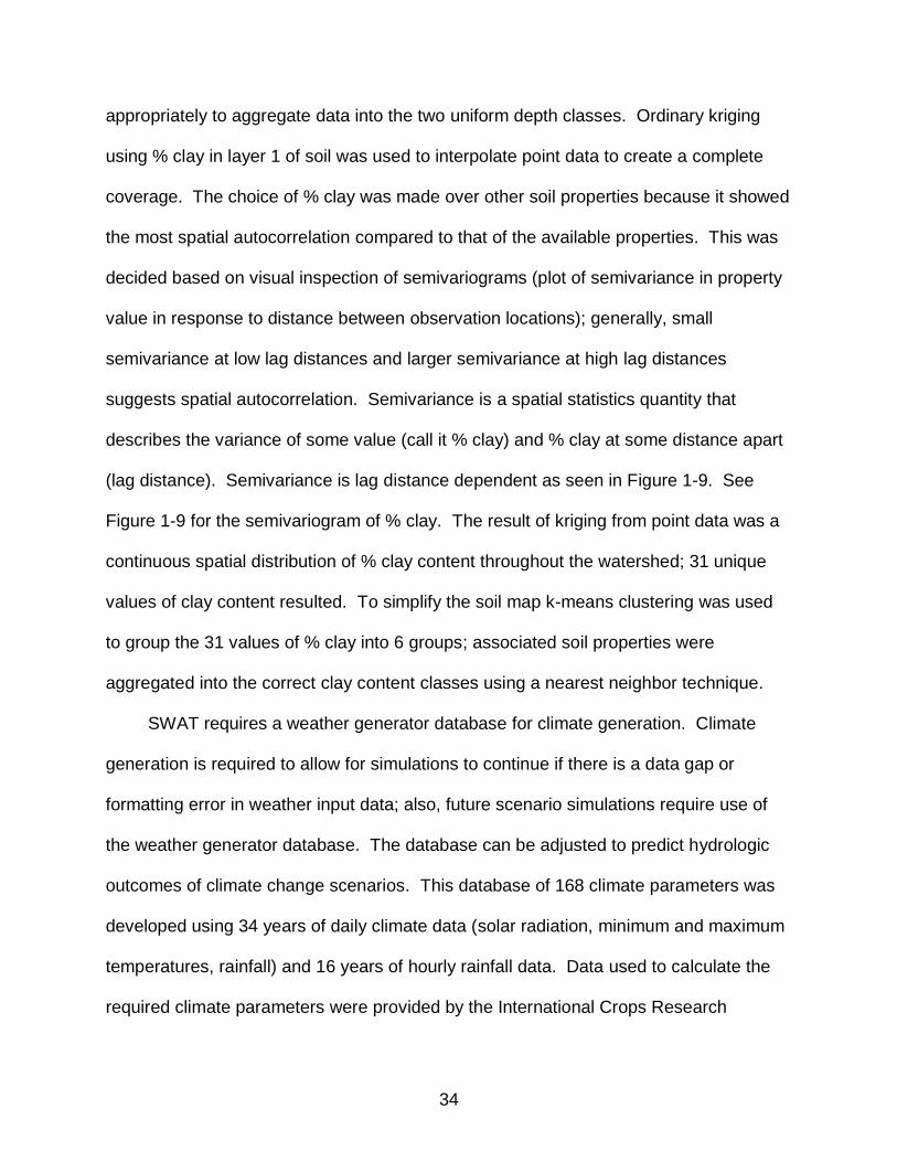
appropriately to aggregate data into the two uniform depth classes. Ordinary kriging
using % clay in layer 1 of soil was used to interpolate point data to create a complete
coverage. The choice of % clay was made over other soil properties because it showed
the most spatial autocorrelation compared to that of the available properties. This was
decided based on visual inspection of semivariograms (plot of semivariance in property
value in response to distance between observation locations); generally, small
semivariance at low lag distances and larger semivariance at high lag distances
suggests spatial autocorrelation. Semivariance is a spatial statistics quantity that
describes the variance of some value (call it % clay) and % clay at some distance apart
(lag distance). Semivariance is lag distance dependent as seen in Figure 1-9. See
Figure 1-9 for the semivariogram of % clay. The result of kriging from point data was a
continuous spatial distribution of % clay content throughout the watershed; 31 unique
values of clay content resulted. To simplify the soil map k-means clustering was used
to group the 31 values of % clay into 6 groups; associated soil properties were
aggregated into the correct clay content classes using a nearest neighbor technique.
SWAT requires a weather generator database for climate generation. Climate
generation is required to allow for simulations to continue if there is a data gap or
formatting error in weather input data; also, future scenario simulations require use of
the weather generator database. The database can be adjusted to predict hydrologic
outcomes of climate change scenarios. This database of 168 climate parameters was
developed using 34 years of daily climate data (solar radiation, minimum and maximum
temperatures, rainfall) and 16 years of hourly rainfall data. Data used to calculate the
required climate parameters were provided by the International Crops Research

35
Institute for the Semi-arid Tropics (ICRISAT; Singh, 2009). This was the nearest (45 km
distant) source of a long record of quality climate data, and inspection of annual
average rainfall totals suggests there is little climate difference between ICRISAT and
Wargal. Temperatures, relative humidity and rainfall were measured in Wargal for input
to SWAT for calibration and validation periods. Weather generator database location
was listed in the Wargal watershed as 17.76472 N, 78.62447 E and elevation of 600 m.
2. Design and installation of hydrologic/climate monitoring systems
Climate data for SWAT input and watershed runoff data for model calibration and
validation are summarized in Table 1-2. Rainfall observations were collected manually
and automatically. Automatic rainfall collection, using a tipping bucket gage that logged
each 0.25 mm of rainfall, allowed for hourly precipitation data for GAML infiltration
simulation in SWAT. Sub-daily data were generated from measured daily rainfall for
wet days by HYETOS, a program for disaggregation of daily rainfall data to hourly data
(Koutsoyiannis and Onof, 2001) for periods when hourly rainfall data were unavailable;
there were 6 months in 2010 – due to maintenance problems with the automated rain
gage – during which HYETOS was required to disaggregate daily rainfall observations
into hourly data. HYETOS uses the Bartlett-Lewis pulse based method to generate
storms from daily data based on 6 monthly parameters developed from a record of
hourly data. Hourly data from nearby ICRISAT (Singh, 2009) were used to calculate the
6 Bartlett-Lewis parameters. Disaggregated rainfall will not match actual hourly data,
but it was the best option available given the instrumentation challenges in the Wargal
watershed. HYETOS disaggregated rainfall has been shown to closely match
observations (Rodriguez-Iturbe et al., 1988; Koutsoyiannis and Onof, 2001). Manual

36
daily rainfall was collected at 15 non-evaporating gages distributed throughout Wargal.
Groundwater levels were monitored in 6 borewells and 3 open wells using an electronic
depth sounder. One of the borewells was monitored continuously with a pressure
transducer.
Six reservoirs are found in the Wargal study area; these are water-harvesting
structures excavated long ago that serve to increase groundwater recharge. The
largest of these reservoirs, Kothakunta, is found at the outlet of the watershed and
creates a generally closed watershed, meaning there is rarely outflow other than
percolation of the tanks. Observations of water in Kothakunta reservoir were the data
used for SWAT calibration and evaluation. The area and depth of water in Kothakunta
reservoir, at the outlet of the study area, was monitored using GPS waypoint data and a
staff gage that was manually read weekly or more frequently during rainy periods. A
GPS was used to weekly mark the perimeter of the flooded area of the reservoir by
walking around the reservoir at the water line and recording waypoints. Topographic
survey data were used to develop the depth to volume and area to volume relationships
required to convert observations to storage volume. Increases in storage volume during
a time interval are interpreted as the outflow of the study area as this reservoir stores all
outflow. Only one reservoir was monitored as a “runoff” gauge due to limited personnel
available for data collection. It was decided that one target for calibration was sufficient
given the small size of the watershed; this is commonly done in hydrologic modeling.
Also, recharge observations allowed an additional evaluation measure to further test the
performance of SWAT.

37
Irrigation pumping could be not be sampled in a large number of fields, but 4
borewells were monitored with flowmeters to record irrigation pumping for a small
sample of the most commonly irrigated crops: rice and vegetables. It is expected that
for farmers with functional borewells there is little variability in irrigation depths for a
given crop due to the management of irrigation that is generally dependent only on
electricity supply. Chapter 4 details the irrigation management setup in SWAT and
presents the irrigation observations used.
3. Setup and initialization of hydrologic model. SWAT setup consisted of input
of formatted landscape data (soils and topography and land use) and weather data.
Cropping system management was parameterized through tillage specification, planting
dates, crop selection, and irrigation management. An initialization period of about a
year and half (using some simulated and some measured weather data) was used to
establish more suitable initial soil moisture and reservoir level conditions.
4. Model calibration and evaluation. This step provided quantitative information
on the uncertainty of simulated water balance components at the watershed scale using
observed reservoir storage volume at the outlet of the watershed as the calibration
target. 13 of the most important parameters – based on expert knowledge and
sensitivity analyses of SWAT in the literature – were adjusted to improve accuracy of
prediction of outflow (Chapter 4). Based on the recommendations of Moriasi et al.
(2007), the 3 quantitative statistics being used for model calibration and evaluation were
the Nash-Sutcliffe efficiency (NSE), percent bias (PBIAS), and the ratio of the root mean
square error to the standard deviation of measured data (RSR).

38
5. Water balance simulations of alternative cropping systems. This step
completed the simulation experiments by estimating the resulting water balance
components of cropland management combinations in Wargal. Alternative farm
management scenarios were created by combining tillage, crop selection, and irrigation
management options, based on accepted water conservation strategies and
participation of community members; these alternative management options are
detailed in Chapter 4. A 10-year simulation using generated weather data was used to
develop water balance predictions for existing management and also for all alternative
management options.
6. Evaluation of alternatives. Groundwater recharge, evapotranspiration (ET),
surface runoff, and irrigation withdrawals were among the outputs used to select
management strategy combinations of greatest potential for groundwater quantity
improvement. Chapter 4 provides details on the comparison of management
alternatives.
Hydrology in Ungauged Basins
The International Association of Hydrological Sciences (IAHS) has launched a
decade-long program (2003-2012) called Predictions in Ungauged Basins, or PUB
(Sivapalan et al., 2003). The central goal of this initiative is to reduce predictive
uncertainty of hydrologic models by improving hydrologic process understanding,
developing ways to generalize hydrology among similar watersheds, and increasing the
available hydrologic and landscape data. This research contributes to the goals of PUB
by improving a hydrologic model through increasing the physical basis of the infiltration
routines with the addition of a parameter which can be expected to have much lower
uncertainty and variability than the other soil properties important for infiltration

39
prediction: effective hydraulic conductivity and wetting front suction. Also, the use of
small surface reservoirs as runoff gages increases the evidence for this being an
effective strategy for acquiring data for model calibration and evaluation in the absence
of streamflow measurements.
Factors Influencing Groundwater Recharge: Literature Review
Of the roughly 35 million km3 of freshwater on Earth, 69% is frozen in glaciers and
permafrost, and of the remaining 31% of global freshwater resources 96% occurs as
groundwater – the rest is divided between surface water and soil moisture
(Shiklomanov, 2000). An important objective of this research is to understand how the
groundwater balance can be managed through reductions in irrigation withdrawals and
increases in recharge through tillage management. The following sections review a
variety of literature on groundwater recharge to assess which factors have the greatest
influence on recharge.
Groundwater recharge is primarily controlled by climate, topography, soil
properties, land use/land cover, and geology (Rushton, 1988; Le Maitre et al., 1999;
Delin et al., 2000; de Vries and Simmers, 2002; Lin et al., 2007). The following review
of literature attempts to select the dominant factor(s) for a given climate/region. The
strength of correlations between groundwater recharge and soil properties, topography,
geology, and land use/ land cover (LULC) are compared, qualitatively, from a review of
research on groundwater recharge estimation and prediction.
Rationale and Significance of a Groundwater Recharge Literature Review
The two main issues having management implications associated with
groundwater recharge are groundwater contamination (quality) and groundwater
depletion or overdraft (quantity) (Lerner et al., 1990). Groundwater is the main source

40
of water for agricultural, municipal, and industrial uses in some parts of the world;
therefore, the quantity and quality of groundwater is of great importance and is the focus
of management efforts. Cities or villages that depend on groundwater for domestic
supplies are vulnerable if groundwater supplies become of insufficient quantity or
quality; water has to be imported or purified to meet domestic supplies. The same is
true for farming systems and industries that depend on groundwater.
Groundwater can be managed by changing water fluxes at the land surface by
altering soil properties (organic or mineral amendments), topography (water harvesting
ponds, tillage), or LULC (impervious area, types of vegetation). Subsurface flows can
also be altered by modifying geology through recharge and discharge structures that
penetrate confining or slow-flowing formations; groundwater withdrawals for agricultural,
municipal, or industrial supply do of course influence subsurface flows. It is sometimes
desirable to increase groundwater recharge to meet increased withdrawal demands,
and it is sometimes the goal to decrease groundwater quantity to prepare for
construction or relieve waterlogging and/or salinity problems in croplands. Managing
anything well requires information about the quantity of interest and the relevant
processes; therefore, it is helpful to know which factors related to groundwater recharge
are the most important to consider. To summarize, the objectives of this review are:
Compare correlations of the four manageable factors – soil properties, topography, geology, LULC – to groundwater recharge
Determine if there is consensus in the literature on the factor that dominates groundwater recharge (locally)
Find methods of recharge measurement/estimation that are most regularly used

41
Land Surface Environmental Factors and Groundwater Recharge
With a focus on the four manageable, environmental factors being considered,
three synthesis papers were selected to evaluate the prevalence of factors considered
for groundwater recharge. Two of the reviews were selected to approach groundwater
recharge from different perspectives. The first perspective is that of vulnerability
assessment, contamination, and water quality (Gogu and Dassargues, 2000); the
second perspective is that of recharge processes, estimation, and quantity (de Vries
and Simmers, 2002). The third review covers an extensive range of study areas and
summarizes recharge rates and controls among them. Qualitative comparisons are
made of these reviews to examine the frequency of consideration of the four factors in
the studies included in each review. Additionally, nine studies of groundwater recharge
relationships to the three most manageable of the four factors (soils, topography, LULC)
were sampled and reviewed for comparison. These papers (published in the last 10
years) were summarized and their methods and outcomes tabulated for comparison.
Groundwater quantity and quality are well connected because the same factors
that make a groundwater system vulnerable to quality degradation can improve
groundwater recharge or quantity; areas of greater groundwater recharge are the areas
that are most vulnerable to contamination. Ten methods of vulnerability assessment
are reviewed by Gogu and Dassargues (2000); references and variables included for
vulnerability assessment are given in Table 1-3.
The outcome of a vulnerability analysis is a quantitative measure (often a map) of
groundwater vulnerability to contamination; however, the measure of vulnerability is just
a number – some type of index – that is relative to other vulnerabilities predicted with
the same method. There is no absolute vulnerability quantification. The most thorough

42
methods are the DRASTIC and SINTACS approaches which both use the following
seven parameters for vulnerability classification: depth to water, net recharge, aquifer
media, soil media, topography, impact of the vadose zone, and hydraulic conductivity.
The review by de Vries and Simmers (2002) suggests climate, geology,
topography, soil condition, and vegetation are the factors determining groundwater
recharge. Geology control of recharge is illustrated by the case of recharge differences
in Botswana between the Kalahari sands and the adjacent Precambrian hard-rock area.
Rainfall in the two areas is similar (300 – 500 mm/year); tracer observations and
modeling estimates show similar recharge in the Kalahari sands (1-10 mm) and hard-
rock areas (10-30 mm). However, spatial distribution of recharge is very different
between the two areas. The hard-rock area shows about 50% of recharge occurring
through preferential flow from fractured rock, creating small (5-10 km2) groundwater
basins that often coincide with morphologic (read: topographic) depressions.
Groundwater recharge in the Kalahari sands is more spatially uniform, having less
variability of soil moisture in the vadose zone and little geologic control of recharge.
A very thorough review of 98 groundwater recharge studies reported in the
literature was completed by Scanlon et al. (2006) focusing on recharge in arid and semi-
arid regions. Their conclusions are summarized in the following three sentences. The
chloride mass balance technique is the most widely used method for estimating
recharge. LULC change is the factor most regularly controlling recharge: in Niger LULC
changes resulted in recharge responses that greatly exceeded those resulting from
climate variability, including severe droughts; in Australia, deforestation has resulted in
recharge increases of 2 orders of magnitude, causing severe groundwater salinity

43
problems due to the flushing of the large amounts of chlorides present in soils. The
authors suggest that high sensitivity of groundwater recharge to LULC means that
recharge can be managed in most cases by LULC changes.
Land use and land cover
Groundwater recharge in arid and semiarid regions is typically small relative to
other water balance components. Rainfall distribution in these areas is characterized by
marked wet and dry periods; the wet periods having storms of significant intensity. The
result of these precipitation patterns is that groundwater recharge is largely episodic (de
Vries and Simmers, 2002). Episodic recharge describes groundwater recharge events
of low frequency and large relative contributions. This type of recharge is highly
sensitive to topography and difficult to manage through vegetation changes (de Vries
and Simmers, 2000; Zhang et al., 1999).
The conversion of native vegetation to annual cropping systems in southeastern
Australia has increased groundwater recharge and caused salinity problems as a result
of rising water tables. To assess the impact of agronomic practices (vegetation type) on
groundwater recharge, Zhang et al. (1999) used a biophysically based water balance
model (WAVES) at two sites in Australia to simulate water balance components in
response to changes in crop rotation and type. Their simulations showed that
perenializing croplands and growing crops having greater rooting depth did decrease
occurrence of small recharge events and overall recharge. Vegetation management
was able to reduce annual recharge amounts by elimination of fallows and increased
root depths. At one location, simulating two different rotations, a change to a deeper
rooting variety (0.5 m depth to 1.0 m depth) resulted in reduction in annual recharge of

44
50%. The main conclusion was the recommendation that fallows be replaced with
vigorously vegetative crops to reduce recharge.
Water flows in the Dill Catchment, Germany were simulated to estimate sensitivity
of flows to vegetation and soil property changes associated with vegetation changes
(Huisman et al., 2004). Water flows considered were total runoff, actual
evapotranspiration, surface runoff and ground water recharge; vegetation scenarios
were pasture (perennial) and cropland (annual): cropland was a common rotation of
summer barley, winter rape, and winter wheat. A quantity called distinction level was
used to compare hydrologic responses to vegetation change. The distinction level
helps compare the sensitivity of the simulated hydrologic fluxes to soil and vegetation
parameter changes relative to the uncertainty in these fluxes due to parameter
uncertainty. The results showed very little sensitivity of hydrologic fluxes to soil
properties (saturated hydraulic conductivity, bulk density, available water content, depth
of top soil layer). For the study area, groundwater recharge was little affected by
changes from cropland to pasture because the opposite effects on runoff and
evapotranspiration. Higher evapotranspiration and lower runoff amounts resulted from
shifts of cropland to pasture (replacing 50% of cropland with pasture – runoff: 596.9 to
536.0 mm/yr; ET: 292.9 to 352.8 mm/yr).
Groundwater recharge and baseflow were estimated for the Upper Mississippi
River basin (Arnold et al., 2000) using the Soil and Water Assessment Tool (SWAT) and
two data analysis methods (recursive filter to separate baseflow from daily flow and
hydrograph recession displacement to estimate groundwater recharge). Groundwater
recharge, runoff, baseflow, and ET were most sensitive to (in order of decreasing

45
sensitivity): Curve Number, soil available water capacity, evaporation compensation
coefficient (adjusts the depth distribution of evapotranspiration from the soil). The
greatest sensitivity to Curve Number is not surprising as this quantity contains
considerable information about land use/land cover.
Topography
It has been shown by Delin et al. (2000) that even small differences in
topography can substantially influence groundwater recharge. Their research site in the
sand plains of central Minnesota was planted in maize under uniform tillage, eliminating
most of the effects on recharge from land use and microtopography differences
between sites. An upland and lowland site were selected, separated by 78 m of
distance and 1.4 m of land surface elevation difference. Three methods for recharge
estimation were used: well hydrograph analysis, unsaturated zone water balance, and
chlorofluorocarbon tracer dating. Mean annual recharge at the site of lower elevation
was greater than recharge at the site of higher elevation by 30% (estimated from
hydrograph analysis), 60% (estimated from water balance), and 80% (estimated from
chlorofluorocarbon dating). These results from a diversity of methods during a 4 year
study suggest that small differences in topography (1.4 m) can be significant factors in
estimation of groundwater.
The resolution of the representation of topography can significantly impact
predictions of land surface processes (Schoorl et al., 2000). Digital elevation models
(DEMs) of the same terrain using different resolutions can result in result in different
predictions of landscape properties or processes. Computational and sensing costs
currently preclude very high resolution DEMs, but the microtopographic relief that they
represent does influence land surface hydrologic processes. The effect on hydrologic

46
simulations of runoff in response to centimeter-scale representations of a landscape
were considered by Martin et al. (2008); interpolated at resolutions of 0.75 cm, 10 cm,
25 cm, 50 cm, 75 cm and 100 cm for vegetated and bare surfaces of a 20 m x 10 m
slope in British Columbia, Canada. Elevations were obtained from a ground-based
laser scanner. Their results showed marked decreases in mean depression storage
(MDS) for the landscape with increasing DEM grid size. From 0.75 cm resolution to 25
cm resolution, MDS decreases from 2.4 cm to 1 cm, and is negligible at resolutions
above 25 cm. They demonstrate the infiltration/runoff partitioning changes in response
to varying MDS, making clear the implications for groundwater recharge.
The strength of topography as a predictor of groundwater recharge was
quantified by Bakhsh and Kanwar (2008) in their study of landscape attributes and their
correlation to subsurface drainage clusters. Flow data from measurements of
subsurface drainage (pipes below agricultural fields) was used to find the landscape
attributes (soil type, elevation, slope, aspect, curvature, flow length, flow direction, and
flow accumulation) that best explained flow variations. Thirty-six plots in a field each
had their own drainage outlet and subsurface flow was measured from each plot. While
subsurface flow was occurring laterally through drainage pipes, it was essentially deep
drainage or potential groundwater recharge that was being intercepted. Stepwise
discriminant analysis was used to select the attributes that made the biggest
contribution to subsurface flow. Elevation and flow accumulation were both selected as
the attributes that best explained the spatial variability of subsurface flows. Three soil
types were classified for the site; saturated hydraulic conductivity was considerably

47
different among them (35 – 100 mm/hour), but the analysis only selected topographic
variables as having strong correlation with subsurface drainage flows.
Soil properties
Sensitivity analysis of groundwater recharge to numerous soil and vegetation
parameters was completed using a simple one dimensional water balance with weather
and vegetation information for England (Finch, 1998). One-at-a-time sensitivity analysis
was used: all parameters being held at their mean values while the parameter of
interest varies across its specified range. Numerous vegetation parameters were
considered for three vegetation types, and mean annual recharge was estimated at
176.7, 290.5, and 96.4 mm for permanent short vegetation, annual short vegetation,
and forest, respectively. Water balance simulations showed greater sensitivity of
groundwater recharge to soil parameters (available water content, root zone depth)
than to vegetation parameters (leaf area index, canopy height, growing season length).
The simplified water balance model estimates runoff as 10% of rainfall if a rainfall event
is greater than 5 mm; topography and a physically-based description of infiltration/runoff
processes were ignored for the purposes of the study.
A method for estimating groundwater recharge in southern India was tested by
Anuraga et al. (2006) using a soil-water-atmosphere-plant model able to describe land
use and soil types. Soil data for the study area of Bethamangala subwatershed was
simplified into two classes: one sandy loam (Type 1) and one clay (Type 2). Annually,
average recharge for the soils was 212 and 99 mm for the sandy and clayey soils,
respectively; this difference is claimed to be due to the higher evaporative losses from
the clay soil as a result of its higher water holding capacity. Annual water balances for
three cropping intensities were simulated. Type A: Finger millet, potato, and tomato are

48
cropped during kharif, rabi, and summer seasons, respectively: total amount of irrigation
is 410 mm/year. Type B: Finger millet is cropped during kharif season with
supplemental irrigation of 150 mm/year. Type C: Finger millet is cropped during the
kharif season without irrigation. Recharge for sandy and clayey soils, respectively, for
cropping systems were 220 and 90 mm/year for system A, 232 and 124 mm/year for
system B, and 184 and 84 mm/year for system C. This suggests that soil texture
influence on recharge is strong.
A single-layer soil water balance model, developed by Eilers et al. (2007) was
used to estimate groundwater recharge during a 36 year period in semi-arid northeast
Nigeria. The model includes 11 soil and 13 vegetation parameters that are not spatially
distributed. Simplicity and low data requirements of the model are touted as its
strengths, and it is promoted for use in cropland areas for water management purposes.
The simulated water balance was used to find sensitivity of groundwater recharge to
model inputs and parameters. Total available water (TAW), followed by rooting depth
and then by crop coefficient, was found to be the parameter with the greatest effect on
simulated recharge. TAW depends both on soil properties and plant rooting depth.
Near surface storage (NSS) depth was also shown to significantly influence recharge.
Quantifying Groundwater Recharge
Methods for quantifying groundwater recharge can be grouped into 3 categories:
physical, tracer, and numerical modeling (Scanlon et al., 2002). These methods are
used differently in surface-water based studies, unsaturated zone studies, and
saturated zone studies. Table 1-4 summarizes the various methods for measuring and
estimating groundwater recharge. In this study in the Wargal watershed, unsaturated
zone water-balance modeling is used to estimate groundwater recharge using a

49
distributed solution to the water balance equation at the surface and in the unsaturated
zone. Deep drainage, water percolating below the root zone is assumed equivalent to
groundwater recharge. This equivalency assumption is valid based on the limited
surface-water/groundwater connections and the substantial depth to groundwater.
Seepage meters, lysimetry, and tracers all only give point estimates, and sufficient point
estimates to distribute groundwater recharge in the 500 ha study area would be too
costly. The water-table fluctuation method would not be effective because of the
amount of groundwater pumping and number of wells (190); it would not be possible to
have a sufficient number of groundwater wells that were uninfluenced by groundwater
pumping.
Discussion and Conclusions on Factors Influencing Groundwater Recharge
The studies considered in this review span a range of locations and climates,
making it difficult to make a rigorous comparison of correlations (groundwater recharge
to soil properties, topography, geology, LULC). This review can, however, suggest
environmental factors having the greatest correlation to recharge in a certain region.
Table 1-5 summarizes the papers reviewed in this section: giving their location, the
factors considered, and the factor explaining most of the variability in groundwater
recharge. The dominance of simulated water balances in experimental methods is not
uncommon in groundwater recharge studies, and it affirms the use of water balance
simulations in the Wargal study area. Measured water balances are difficult as
determination of boundary conditions of a groundwater system generally requires vast
instrumentation for measurement of surface and subsurface quantities (including
descriptions of geology) both in the study area and in surrounding areas. Tracer mass
balances seem to be the most effective way of estimating local recharge; seepage

50
meters can also provide accurate point estimates of recharge. The prevalence in the
literature of simulation tools for estimating sensitivity of groundwater recharge to
environmental factors supports the use of SWAT in this analysis to estimate
groundwater recharge under current and modified management.
This review and the extensive review by Scanlon et al. (2006) suggest that land
use and land cover has the most control over recharge processes within a given
climate. In 4 of the 9 studies tabulated above, a quantity related to LULC dominates
groundwater recharge control. In 3 of the 9 studies, a topographic quantity was found to
be most influential on groundwater recharge. Of the 6 studies that considered LULC
there were 2 which find a soil property having a greater influence on recharge. For
agricultural areas, the sensitivity of recharge to LULC suggests that cropping system
changes can have significant effects on groundwater recharge.
Options for Managing Groundwater in Agricultural Systems
Recall the water balance discussion in the earlier section, “Groundwater Balance
and Agricultural Management”. Equation 1-1 described the water balance of the
unsaturated zone and at the soil surface: ∆SW = P + I – ET – RO – ∆SS – DP + ∆UF,
where SW is soil water, P is precipitation, I is irrigation, ET is evapotranspiration, RO is
runoff, ∆SS is a storage pool representing the increase or decrease in surface storage
in small or large depressions, DP is deep percolation, ∆UF is the net change in
subsurface flow into and from the system.
Equation 1-2 described the water balance in the saturated zone (groundwater
system): ∆S = R – I – CR + ∆SF, where S is groundwater storage, R is recharge
(approx. = DP), I is irrigation pumped from groundwater, CR is capillary rise, ∆SF is the
net change in flow into and from the groundwater system. As discussed earlier, if the

51
goal is to improve or maintain S (groundwater storage), then it is essentially irrigation
and recharge that remain as the manageable quantities in the groundwater balance.
These quantities appear in the surface water balance as I and DP. Decreasing
irrigation pumping (I) could be done through a variety of possible management changes:
providing supplemental rather than full irrigation, irrigating only at critical phenological
times, changing crop planting date to increase effective rainfall, choosing crops with
lower water requirements, or improving application technology. At the farm-scale,
efforts to increase recharge (DP) include: excavating farm ponds, using zero or reduced
tillage, mulching, and tillage for water harvesting (tied-ridging, contour bunding, and
others). All these techniques can increase groundwater recharge by increasing surface
water storage depth which allows for longer infiltration times of excess rainfall. The
above review of groundwater recharge studies highlights the difficulties associated with
measurement of groundwater recharge and the prevalence of water balance models for
use in simulation of recharge.
Contributions of this Research
There are four major contributions that make this research significant. (1) The
improvement of the GAML infiltration process description in SWAT to include surface
storage depth as a time-varying head and as a storage term at the surface. This allows
for evaluation of water harvesting tillage and enables flooded croplands (rice) to be
simulated with the use of SWAT’s land use update routines (lup.dat), which allow for
dynamic cropland areas to represent management changes and intensive cropping
sequences. This improved infiltration description has a stronger theoretical basis than
the typical GAML formulation used in SWAT and similar hydrologic models, and
sensitivity analyses (Chapter 3) have shown that infiltration predictions are sensitive

52
(rank 2 of 5 parameters) to the parameter describing maximum depression storage in
systems having non-negligible surface storage depth. (2) The use of lup.dat in SWAT
for sequences of multiple crops in a single year, common in semi-arid and tropical
ecosystems, and for implementing cropping system changes is unique in its application
here. Typically this functionality is used for long term (decade-scale) and broad land
use change; for example, conversion of unmanaged forests to annual croplands. Here,
it is used for the first time (according to lead SWAT model developer: Arnold, 2010) to
model these intensive cropping sequences. (3) The use of reservoir storage volumes
for calibration and evaluation of model predictions in a small watershed with little
convergent surface flow is an innovative strategy for data acquisition and model
application in an ungauged basin (Chapter 4; Liebe et al., 2009). Small reservoirs for
irrigation use and groundwater recharge are common in India and in some areas of
Africa; this research demonstrates an effective, inexpensive way to use these surface
water bodies to calibrate and evaluate hydrologic models in watersheds without records
of streamflow. (4) This research quantifies the impact of rice croplands on the
groundwater balance at the landscape scale in a typical semi-arid Indian watershed. In
recent years there has been growing awareness, publicly and in the scientific literature,
that groundwater depletion is becoming a problem in India (CGWB 2007; Rodell et al.,
2009; Shah, 2007), but there is no information on the extent of irrigated croplands
(largely rice) allowable for groundwater sustainability.

53
Figure 1-1. Study area location in Wargal mandal, eastern Medak district, northwestern Andhra Pradesh

54
Figure 1-2. Groundwater system diagram of Wargal (adapted from Dewandel et al., 2006 and Marechal et al., 2006). t is layer thickness, values are approximate. Water table height fluctuates between 15 and 35 m below surface.

55
Figure 1-3. Water balance diagram showing connections between unsaturated and saturated zone water balances. I is irrigation, P is precipitation, SS is surface storage, Inf is infiltration, ET is evapotranspiration, RO is runoff, UF is unsaturated flow, CR is capillary rise, R is groundwater recharge, DP is deep percolation, SF is saturated flow.

56
Figure 1-4. Total annual harvested areas of rice in India and Andhra Pradesh, 1961-
2001
Figure 1-5. Area equipped for mechanized irrigation from groundwater source in India:
1961, 1971, 1981, 1986, 1993; population of India each year from 1961 to 2007.
0
0.5
1
1.5
2
2.5
3
3.5
4
4.5
5
0
5
10
15
20
25
30
35
40
45
50
1960 1970 1980 1990 2000
AP
ric
e a
rea,
Mha
India
ric
e a
rea,
Mha
India rice cropland areaAndhra Pradesh rice cropland …
0.46
1.16
7.30
11.90
17.70
20.60
26.54
0
5
10
15
20
25
30
0
0.2
0.4
0.6
0.8
1
1.2
1.4
1960 1970 1980 1990 2000
Gro
undw
ate
r irrigate
d a
rea,
Mha
Popula
tion o
f In
dia
, bill
ion
population of India
groundwater irrigated area

57
Figure 1-6. Annual rainfall in Telangana region (1960 – 2008): slight declining trend
observed (about 3 mm/year reduction in annual rainfall if trend is assumed linear)
Figure 1-7. Annual rainfall trends (1960 – 2008) in the 3-state region of the GRACE
study of Rodell et al., 2009
y = -2.8424x + 6552.6
0
200
400
600
800
1000
1200
1400
1960 1970 1980 1990 2000 2010
Annual ra
infa
ll depth
, m
m
year
Telangana annual rainfall
0
200
400
600
800
1000
1200
1960 1970 1980 1990 2000 2010
Annual ra
infa
ll depth
, m
m
year
Punjab annual rainfallHaryana annual rainfallE. Rajasthan annual rainfallW. Rajasthan annual rainfall

58
Figure 1-8. Watershed boundary, reservoir locations (large dots), and digital elevation
model of Wargal watershed, 2.2 m resolution
Table 1-1. Areas (ha) of cropland for three-crop rotation in Wargal
kharif
rabi
summer
ha ha ha
maize 65.96 potato 40.96 beans 10.30
cotton 65.14 sunflower 23.36 beans 10.30
rice 92.63 rice 60.60 beans 10.30
range 288.41 range 387.21 range 481.23

59
Figure 1-9. Variogram plot of % clay in layer 1 of Wargal soil: used to evaluate spatial
autocorrelation of soil properties and for kriging to generate continuous map of soil data

60
Table 1-2. Climate and hydrologic monitoring systems: observation numbers, frequency, purpose
Observation Collection method and number of observations
Frequency Purpose
Rainfall continuous, automated (1) and manual (15)
bi-weekly (continuous) and weekly (manual)
input for hydrology model
Weather Parameters (Solar radiation, wind speed, and temperature)
manual (1) daily input for hydrology model
Reservoir depth and area
staff gage: manual reading (1)
weekly (daily during rainy periods)
calibration of hydrology model
Drain flows to tanks water level recorder in flumes: continuous, automated (2)
weekly calibration of hydrology model
Groundwater levels pressure transducer: continuous, automated (1) and sounder: manual (9)
bi-weekly (continuous) and weekly (manual)
calibration of hydrology model
Irrigation pumping flowmeters on borewells: manual reading (4)
weekly input for hydrology model
Table 1-3. Sources and factors included in analysis by Gogu and Dassargues; adapted from Gogu and Dassargues 2000
Reference and model name Parameters
Topography Soils Geology LULC
Albinet and Margat, 1970
• Goossens and Van Damme, 1987
• •
Carter and Palmer, 1987
• • Foster 1987, GOD
•
Aller et al., 1987, DRASTIC • • • Navulur and Engel, SEEPAGE
• •
Civita, 1994, SINTACS • • • •
Van Stempvoort et al., 1993, AVI
• Civita and De Regibus, 1995, ISIS • • • •
Doerfliger and Zwahlen, 1997, EPIK • • • •

61
Table 1-4. Summary of methods for quantifying groundwater recharge
Physical Tracer Numerical Modeling
Surface-water Based Studies
channel water budget, seepage meters
heat, isotopic water balance simulation
Unsaturated Zone Studies
lysimetry, zero-flux plane, Darcy's law
applied, historical, environmental
water balance simulation
Saturated Zone Studies
water-table fluctuation, Darcy's law
historical, environmental
water balance simulation

62
Table 1-5. Summary of the 9 recharge studies highlighting dominant factors
Study area; Reference
Factors: *most important Experimental methods
southern India; Anuraga et al., 2006
soil*, LULC (cropping system) distributed simulation
Upper Mississippi River Basin; Arnold et al., 2000
soil, LULC* distributed simulation
Nashua, Iowa; Bakhsh and Kanwar, 2008
soil, topography (elevation*, slope, aspect, curvature, flow length, flow direction, flow accumulation*)
drain flow measurement
Central Minnesota corn field, Delin et al., 2000
topography(elevation*), soil simulation, tracers, well hydrographs
Wallingford, UK; Finch, 1998
soil, LULC (LAI*, stomatal resistance, rooting depth, AWC)
local simulation
northeast Nigeria; Eilers et al., 2007
soil (total available water*), LULC (rooting depth, Kc)
local simulation
Dill catchment, Germany; Huisman et al., 2004
soil, LULC (cropping system*) distributed simulation
British Colombia, Canada; Martin et al., 2008
topography (DEM resolution*) distributed simulation
Mallee, SE Australia; Zhang et al., 1999
LULC (rooting depth*, fallowing) distributed simulation

63
CHAPTER 2 RAINFALL INTENSITY-DURATION-FREQUENCY RELATIONSHIPS FOR ANDHRA PRADESH, INDIA: CHANGING RAINFALL PATTERNS AND IMPLICATIONS FOR
GROUNDWATER RECHARGE
Rainfall Characterization and Water Resource Management
The development and maintenance of rainfall intensity-duration-frequency (IDF)
relationships is important for a variety of water-related design and management,
including flood control, energy generation, water supply, agricultural drainage, and
others. With growing competition for freshwater resources in much of the world, the role
of updated IDF relationships for application in developing innovative water management
strategies is becoming increasingly important. Improved characterization of rainfall,
through updated IDF relationships, has been shown to improve water resource planning
and management decisions (Karl et al., 1995; Angel and Huff, 1997; Guo, 2006). For
example, a case study of Chicago urban drainage systems showed that drainage
systems designed using updated IDF relationships, using shorter records of more
recent data, performed significantly better than those developed from older rainfall
records (Guo, 2006).
There is mounting evidence from global and regional studies that precipitation
patterns are shifting toward more common higher intensity storms and fewer light and
moderate events (Kunkel et al., 1999; Easterling et al., 2000; Trenberth et al., 2003;
Goswami et al., 2006; Joshi and Rajeevan, 2006). These observed changes in rainfall
characteristics suggest that IDF analyses be regularly updated to include more recent
and shorter records of rainfall time series and exclude older, less-representative data.
The analysis of Trenberth et al. (2003) notes that the Clausius–Clapeyron equation
relating vapor pressure and temperature suggests a 7% increase in atmospheric water

64
content for each ⁰C increase in average annual temperature. As a result of low-level
moisture convergence, local rainfall rates greatly exceed average regional or global
evaporation rates; therefore, rainfall intensities could be expected to increase at a rate
at least as large as 7% / ⁰C. However, this differs from the accepted 1 – 2% / ⁰C
increase in total annual precipitation depths (IPCC, 2001). To reconcile the differences
in these predictions, it follows that low and moderate intensity precipitation events will
be less common, and precipitation would trend toward less frequent, higher intensity
events (Trenberth et al., 2003). This argument is supported by global climate model
predictions (the UKHI and CSIRO9 general circulation models; Hennessy et al. 1997)
and by an investigation of rainfall records for the large region of central India (Goswami
et al., 2006). Of course the spatial distribution of this change in precipitation character
is uncertain, but it would mean greater risk of both dry spells and floods for some
regions even though annual precipitation totals may increase slightly.
The recent rainfall character study (Goswami et al., 2006) of a large central Indian
region used analyses of daily rainfall data from 1803 stations (1951-2000), and found
significant increases in frequency and magnitude of high intensity rain events (>100
mm/day) and significant decreases in frequency of light and moderate events (>5 and
<100 mm/day). The authors observed that these trends are more difficult to notice
based on analyses from individual station data due to the large variability in daily data.
The regional analysis, however, having much larger sample size due to the large
number of stations, is better able to detect long term trends in rainfall intensity.
Groundwater Resources in India
Groundwater in India is a highly important resource for irrigation and household
use, and its extensive use is resulting in widespread groundwater depletion (Chapter 1

65
“Introduction to Study Area”, Shah et al., 2003; CGWB, 2007; Rodell et al., 2009).
There is general agreement that water scarcity in India is severe (Alcamo et al., 2000;
Yang et al., 2003). Total (761 km3) and agricultural (688 km3) water withdrawals for
India are the highest in the world, and nearly 90% of withdrawals are for agricultural use
(AQUASTAT, 2010). More than half of the irrigation requirements of India are met from
groundwater (CGWB, 2002; Shah et al., 2003), and the number of mechanized
borewells in India has increased from less than 1 million in 1960 to more than 20 million
in 2000 (Shah, 2007). Groundwater in India is a highly important resource for irrigation
and household use, and its extensive use is resulting in widespread groundwater
depletion (Shah et al., 2003; CGWB, 2007; Rodell et al., 2009).
A recent groundwater depletion study (Rodell et al., 2009) in the northwestern
Indian states of Haryana, Punjab, and Rajasthan, is illustrative of common regional
groundwater depletion problems in India. Using the Gravity Recovery and Climate
Experiment (GRACE) satellites to measure changes in terrestrial water storage during
the study period from August 2002 to October 2008, 109 km3 of groundwater loss was
estimated, or about 4 cm each year over the three-state area. In the southern state of
Andhra Pradesh, the Central Groundwater Board (CGWB) of India observed a 2 – 4 m
decline in groundwater levels in 26 observation wells in the Medak district during the 10
years from 1996 to 2005, suggesting an approximate annual decline of about 30 cm
(CGWB, 2007).
Objectives: Precipitation Characterization and Groundwater in India
Considering the importance of groundwater resources in India, it is likely that if
rainfall becomes characterized by more common events of high intensity, the result
would be a higher fraction of rainfall contributing to runoff and a reduced fraction

66
available for infiltration and groundwater recharge (de Vries and Simmers, 2002; Gujja
et al., 2009; Gupta et al., 2010, Rangan et al., 2010). This may put the already reduced
strained groundwater resources of India at even greater risk of depletion.
Several states in northwestern and peninsular India are experiencing groundwater
depletion (CGWB, 2007, Rodell et al., 2009). In Andhra Pradesh, for example, depleted
groundwater supply, resulting from irrigation withdrawal expansions, has severe
consequences for farmers that have invested in borewell infrastructure. Farmers bear
substantial costs of groundwater depletion: greater yield variability, costs of failed
borewells, and the expenses to develop new borewells. Updated IDF relationships that
reflect the changes toward more episodic rainfall in Andhra Pradesh serve to emphasize
the importance of surface storage depth as a management option for increasing
infiltration and groundwater recharge in agricultural areas
An area in northern Andhra Pradesh, in the Medak district is studied here as a
case study to demonstrate the advantages of updated IDF relationships for a region in
India that is facing acute water shortages. The objective of this study is to develop
updated IDF relationships for Hyderabad, Andhra Pradesh, India. These updated
rainfall descriptions are then used to demonstrate the changes in precipitation intensity
and the need for regularly updated rainfall characterizations using recently available
sub-daily rainfall records. The updated IDF relationships are compared to earlier
analyses for the region, and the effects of changing rainfall character on groundwater
resources in India are discussed. These IDF curves can be useful tools for numerous
types of water resource management projects in Hyderabad (a major city in India) and
the surrounding region. For example, in a small agricultural watershed near Hyderabad,

67
the causes and solutions of groundwater depletion, a common regional problem, are
being analyzed (Chapter 4), and these new IDF relationships are being used to improve
predictions of infiltration (Chapter 3) and groundwater recharge.
Rainfall Characterization
Overview of IDF Analysis
Generally, the development of IDF curves follows four main steps. First, rainfall
intensity data are organized into an annual maximum series. This is done for each
duration of interest (1 hour, 4 hour, 8 hour, etc.) by finding the maximum rainfall
intensity for the duration specified for each year. Second, a probability distribution is
fitted to the annual maximum series using any choice of statistical techniques
(maximum-likelihood, l-moments, or other). Third, the cumulative distribution function
(CDF) chosen and parameterized in step two is used to calculate rainfall intensities from
the frequencies (1/probability) desired (2 year, 5 year, 10 year, etc.) for each of the
durations being considered. Fourth, the curves can be fitted to a parametric equation;
this final step is optional and is useful if it is desirable to avoid using multiple CDFs for
rainfall IDF prediction or if IDF curves are to be estimated for durations or frequencies
not in the period of record. A common parametric equation form for IDF curves is
(Bernard, 1932):
(2-1)
where ItT is the rainfall intensity of a combination of T (frequency or return period, years)
and t (duration, hours) and empirically calculated constants A1, A2, and A3.
Limited IDF information is available for India. The study of Kothyari and Garde
(1992), using rainfall data (1950-1980) from 80 recording gages grouped geographically

68
based on rainfall characteristics, provided IDF curves for 5 large regions of India:
northern, central, western, eastern, and southern. The Kothyari and Garde (1992) IDF
relationships are the most current national IDF characterizations for India available in
the literature, their IDF relationships will be used for comparison to those developed
here. Their analysis found that the performance of Equation 2-1 (Bernard, 1932) could
be improved by including some rainfall characteristic (Rchar) in the expression. Four
rainfall properties were considered as candidates for inclusion in the equation:
, where ItT is the rainfall intensity of a combination of T (frequency
or return period, years) and t (duration, hours), Rchar is some rainfall characteristic, and
C1, C2, C3, and C4 are constants fitted to IDF data generated from the CDF which was
fitted to observed data. Options considered for Rchar were mean annual rainfall (R),
mean of the maximum monthly rainfall (Rmax), ratio (R/Rmax), and the 24-hr duration,
two-year return period rainfall depth (R242) were used. It was found by comparing
multiple regression correlation coefficients that R242 was most effective at improving IDF
curve fit to observed data, giving the IDF equation of the form (Kothyari and Garde,
1992):
(2-2)
Methods for Rainfall IDF Development for Andhra Pradesh
Two rainfall time series obtained (Singh, 2009) from recording gages at the
International Crops Research Institute for the Semi-arid Tropics (ICRISAT) near
Hyderabad, Andhra Pradesh, India were used to develop IDF relationships for this
study. The first series consisted of 140,256 records of hourly rainfall (16 year period,
1993-2008); this data series was used for development of IDF relationships. The

69
second rainfall time series consisted of 12,784 records of daily rainfall from (35 year
period, 1974-2008); this data was used to analyze long term trends in occurrence of
threshold-based high intensity rainfall events. Sub-daily rainfall records are important in
rainfall IDF analyses for accurate determination of short duration (2, 4, 8 hour) storm
intensities, and hourly rainfall records for India are sparse and are generally only
available since the early 1990’s (Jain et al., 2007). Average annual rainfall in
Hyderabad is 880 mm, and 75% of that rainfall arrives during the rainy season from
June to September called Kharif. The studies of Indian monsoon rainfall variability
(May, 2004) and spatial coherence of tropical rainfall (Moron et al., 2007) suggest that
the IDF relationships developed here, based on rainfall records from a recording station
in Hyderabad are applicable for the Medak district.
Using the hourly rainfall data, annual maximum series (AMS) for all durations
considered were developed by calculating a moving average intensity for each duration
and then finding the maximum average intensity for each duration during a calendar
year. This is step one of IDF curve development. The Weibull probability distribution
was chosen based on graphical and log-likelihood value comparisons of fit to the AMS
data of Weibull, Generalized Extreme Value, Gamma, and Log-Normal probability
distributions. Maximum likelihood estimation of parameters for the Weibull CDF was
completed independently for each of the five durations (1, 2, 4, 8, and 24 hour); see the
resulting parameters α (Weibull scale parameter) and β (Weibull shape parameter) in
Table 2-2 (this is step two). The two-parameter Weibull probability density and
cumulative distribution functions are:
(2-3)

70
(2-4)
where f is probability, F is cumulative probability, I is rainfall intensity, α is Weibull scale
parameter, and β is Weibull shape parameter. The five resulting CDFs were used to
calculate rainfall intensity for the 5 durations at all the frequencies required; in this case
2, 5, 10, 15, 25, 50, 75, and 100 year return periods were considered (step 3). The IDF
data were then fitted to a parametric equation of the form of Equation 2-2 for
comparison to the Kothyari and Garde (1992) equation to examine the change in IDF
relationships for the region in the last 3 decades.
Exploration of Trends in Occurrence of Rainfall Events of High and Low Intensity
Differences in IDF curves between those developed here and those developed
using older rainfall records (Kothyari and Garde, 1992) can give evidence for a change
in character of precipitation for the region near Hyderabad, India. However, trends in
the total annual numbers of threshold-based high and low/moderate intensity rainfall
events for single recording station can add to the available evidence for changing
rainfall characteristics. Days were counted as high intensity (I) event days if I ≥ 50
mm/day; low to moderate days were those having 5 < I < 50 mm/day. These intensity
classes are commonly used to group rainfall days into high and low/moderate classes
(Angel and Huff, 1997; Goswami et al., 2006). For each calendar year, days in each
class were summed. A longer record was used for this trend analysis than was used for
IDF curve development because of the lack of hourly rainfall data availability and the
decision to use a more recent, shorter record for IDF analysis. Hourly rainfall data give
more reliable IDF relationships, especially for short durations, and most of the available
hourly rainfall records in India begin in the early 1990’s (Jain et al., 2007).

71
Results and Discussion: IDF Curves and Event Intensity Trends
Table 2-1 presents the 1, 2, 4, 8, and 24 hour annual maximum rainfall intensities
for the 16 year record (1993-2008) from which IDF curves were developed. Annual and
rainy season (kharif) rainfall totals and number of rain days are also presented. The
IDF curves developed from the inversion of the fitted Weibull CDF at each duration,
using the various probabilities (1/frequency) and solving for intensity, are plotted in
Figure 2-1. These intensities were used to fit coefficients C1, C2, C3, and C4 to
equation 3-2. Fitting was done separately for each duration and then also for all
durations combined (see resulting constants in Table 2-2); coefficients were fitted using
an automated iterative routine with the goal of minimizing the average root mean
squared error (RMSE) between intensities from the CDF and those from Equation 2-2.
Using the coefficients of Kothyari and Garde (1992) listed in Table 2-2, the RMSE
of rainfall intensities from IDF relationships developed using recent data (1993-2008)
and those calculated from the original Kothyari and Garde formula (1950-1980 rainfall
data) was 28.98 mm/hour. Mean difference (intensities from original Kothyari and
Garde formula minus intensities from newly parameterized Weibull CDF) was -25.43
mm/hour (Table 3-4), and percent difference from the original 1992 formula was greater
than 100% for many return period-duration combinations. This suggests significant
increases in intensity of rainfall events during the last 3 decades for the region near
Hyderabad, India.
Analyzing the daily rainfall data from Hyderabad (1974-2008), noticeable trends
of increasing annual numbers of high intensity rainfall events (I ≥ 50 mm/day) and
decreasing numbers of low and moderate intensity events (5< I <50 mm/day) were
observed (Figure 2-2). These trends have low to moderate statistical significance

72
based on t-tests of the hypothesis of no trend; p-values of 0.27 and 0.082 for slopes of
increasing trend of high intensity events and decreasing trend of low and moderate
events, respectively. The non-parametric Mann-Kendall test of trend significance
showed a significant (α = 0.05) increasing trend for annual numbers of high intensity
rainfall events, but no significant trend for annual numbers of low and moderate intensity
events. The moderate strength of the trends is consistent with the observations of
Goswami et al. (2006) that the high variability of single-gage records makes it difficult to
observe trends of high statistical significance, but the directions of the trends are
consistent with their analysis for all of central India.
Discussion: Precipitation Characterization and Groundwater in India
Changing rainfall characteristics generally have important impacts on the
hydrology of a region. In semi-arid regions, like that of the Hyderabad region, the
annual potential evapotranspiration is much greater than precipitation, runoff generation
is generally Hortonian, and groundwater recharge in these regions depends largely on
high intensity storms and the storage of excess rainfall in surface depressions (de Vries
and Simmers, 2002). Channelized flow is highly seasonal, meaning most groundwater
recharge results from areal infiltration and percolation of surface storage of excess
rainfall. Higher intensity rainfall patterns lead to greater runoff and a lower proportion of
rainfall being infiltrated and available for groundwater recharge. For the agricultural
regions of semi-arid India, groundwater recharge is of major concern: groundwater
depletion is common as a result of substantial irrigation withdrawals. Given the scarcity
and seasonality of surface water resources in the region, increased rainfall variability
makes irrigation from groundwater resources even more important. The evidence
provided by this study suggests rainfall in peninsular India is becoming increasingly

73
characterized by higher intensity events and fewer low and moderate intensity events.
This result has a variety of management applications, but for agricultural areas
dependent on groundwater, one application would be to increase investments in
reservoirs, farm ponds, and water harvesting tillage to increase the infiltration of rainfall.
The value of groundwater resources can be expected to increase when there is more
variable rainfall.
Conclusions on Rainfall Intensity Trends and Groundwater Recharge
Rainfall IDF relationships are useful tools for various hydrologic analyses, and the
updating and maintenance of these relationships is important for decision-making that
requires information about the character of rainfall. The recent evidence of more
common high-intensity rainfall events was extended in this study to illustrate IDF
differences between old and new records and to recommend that IDF relationships be
regularly updated using more recent rainfall records. The newly developed IDF
relationship for the Hyderabad region of southern India, using the formula of Kothyari
and Garde with updated parameters based on 1993-2008 rainfall data, including the 2
year, 24 hour rainfall of 103.2 mm, is
. These new IDF curves
show noticeably greater rainfall intensity patterns – on average 25 mm/hour or 123%
greater for 1 to 24 hour durations – compared to the previously available rainfall
characterization (Kothyari and Garde 1992) for the southern region of India. Based on
this large IDF difference, it is recommended that IDF relationships be regularly updated
to improve decisions and designs that utilize these relationships. These results are
consistent with the growing consensus that precipitation patterns are shifting, especially
in lower latitudes, toward higher intensity rainfall events and a decrease in moderate

74
and low intensity rainfall (Owor et al. 2009; Pall et al. 2006; Trenberth et al. 2003; Allen
and Ingram, 2002). Similar studies of changing IDF relationships using shorter, recent
rainfall records in other regions of India and in other parts of the world could give
increased evidence for changing rainfall characteristics.

75
Table 2-1. Annual maximum series rainfall intensity generated from hourly rainfall data from Hyderabad, Andhra Pradesh, India. Annual and Kharif season (June-September) total rainfall and rain days.
Annual maximum series rainfall intensity, mm/hr Rainfall totals, mm Kharif
1 hour 2 hour 4 hour 8 hour 24 hour Annual Kharif rain days
1993 29.5 17.1 10.0 5.0 2.4 831 588 49
1994 34.8 23.4 14.1 8.9 6.0 848 550 62
1995 54.1 29.9 15.7 7.9 4.0 1266 747 54
1996 50.3 27.8 16.2 11.1 4.7 1063 911 64
1997 29.2 17.8 11.8 7.7 3.9 743 433 48
1998 34.1 21.2 12.0 7.9 2.8 1181 887 64
1999 30.0 16.6 8.7 4.4 1.9 580 455 63
2000 154.9 136.4 105.6 66.0 36.9 2016 1797 66
2001 37.4 20.7 10.5 6.4 2.6 688 514 53
2002 18.5 14.1 7.1 3.8 2.2 623 473 48
2003 50.6 41.2 25.4 12.8 4.3 926 789 66
2004 29.4 26.5 14.3 7.7 3.2 783 546 47
2005 46.7 32.3 18.3 9.3 4.4 1192 850 68
2006 33.8 24.6 17.2 11.9 4.6 889 636 75
2007 30.2 28.4 16.1 8.8 2.9 717 571 77
2008 44.0 25.8 15.6 9.9 7.0 1109 758 65
Table 2-2. Parameters for Weibull CDF: F(I) = 1 - exp(-(I/α))β, where I is rainfall
intensity, and parameters for IDF function:
Weibull CDF parameters IDF function parameters Storm Duration α, scale β, shape C1 C2 C3 C4
1 hour 50.1056 1.6863 7.1068 0.4018 0.2259 0.7100
2 hour 35.2153 1.4214 7.1059 0.4303 0.2614 0.6885
4 hour 21.5984 1.2173 7.1035 0.4264 0.2976 0.6734
8 hour 12.6868 1.1703 7.1025 0.4113 0.3075 0.6686
24 hour 6.0630 1.0670 7.1022 0.4050 0.3318 0.6560
fitted to all 5 durations
7.1052 0.2532 0.4786 0.3889
Kothyari and Garde parameters
7.1000 0.2000 0.7100 0.3300

76
Figure 2-1. Intensity duration frequency curves for 1, 2, 4, 8, and 24 hour durations developed from hourly rainfall data from 1993 – 2008 from Hyderabad, India
Table 2-3. Rainfall intensity values from Weibull cumulative distribution functions (CDFs): hourly data 1993-2008 for Hyderabad
t (hours) T, return period (years)
duration 2 5 10 15 25 50 75 100
1 40.32 66.44 82.16 90.36 100.22 112.51 119.70 123.94
2 27.21 49.22 63.32 70.89 80.15 91.94 98.95 103.12
4 15.98 31.93 42.85 48.89 56.43 66.23 72.17 75.73
8 9.28 19.05 25.87 29.67 34.45 40.70 44.50 46.78
24 4.30 9.47 13.25 15.40 18.13 21.77 24.01 25.37
0
20
40
60
80
100
120
140
0 5 10 15 20 25
Inte
nsity, m
m/h
ou
r
Duration, hours
T= 2 year
T= 5 year
T = 10 year
T = 15 year
T = 25 year
T = 50 year
T = 75 year
T = 100 year

77
Table 2-4. Rainfall intensity (mm/hr) from Kothyari and Garde general formula fitted to recent intensity data (1993-2008) for Hyderabad1. RMSE calculated based on CDF intensities.
t (hours) T, return period (years)
duration 2 5 10 15 25 50 75 100
1 51.40 64.82 77.25 85.60 97.42 116.11 128.66 138.38
2 36.89 46.52 55.44 61.43 69.92 83.33 92.33 99.31
4 26.47 33.39 39.79 44.09 50.18 59.80 66.26 71.27
8 19.00 23.96 28.55 31.64 36.01 42.92 47.56 51.15
24 11.23 14.16 16.88 18.70 21.28 25.37 28.11 30.23
RMSE 6.27
1:
Table 2-5. Rainfall intensity (mm/hr) from Kothyari and Garde original formula fitted to
older intensity data (1950-1980) for southern zone of India1. RMSE calculated based on CDF intensities.
t (hours) T, return period (years)
duration 2 5 10 15 25 50 75 100
1 37.67 45.24 51.97 56.36 62.43 71.71 77.77 82.37
2 23.03 27.66 31.77 34.46 38.16 43.84 47.54 50.35
4 14.08 16.91 19.42 21.06 23.33 26.80 29.06 30.78
8 8.61 10.34 11.87 12.88 14.26 16.38 17.77 18.82
24 3.94 4.74 5.44 5.90 6.54 7.51 8.14 8.63
RMSE 28.98
1:
. RMSE

78
Table 2-6. Differences (mm/hour) in predicted rainfall intensity values between Kothyari and Garde IDF formula using 1992 parameters1 and using updated parameters fitted from this study2
t (hours) T, return period (years) duration 2 5 10 15 25 50 75 100
1 -13.73 -19.58 -25.28 -29.24 -35.00 -44.40 -50.89 -56.01
2 -13.86 -18.86 -23.67 -26.98 -31.75 -39.49 -44.79 -48.95
4 -12.40 -16.48 -20.37 -23.03 -26.85 -33.00 -37.20 -40.49
8 -10.39 -13.62 -16.68 -18.77 -21.75 -26.53 -29.79 -32.33
24 -7.28 -9.42 -11.44 -12.80 -14.75 -17.86 -19.96 -21.61
Mean Difference -25.43
1:
and 2:
Figure 2-2. Annual counts of high (I ≥ 50 mm/day) and light intensity (5 < I < 50 mm/day) rainfall events (1974-2008)
0
10
20
30
40
50
60
0
1
2
3
4
5
6
7
8
9
1970 1975 1980 1985 1990 1995 2000 2005 2010
N(5
<I<
50
mm
/da
y)
N(I
≥5
0 m
m/d
ay)
high intensity events
light intensity events

79
CHAPTER 3 IMPORTANCE OF SURFACE STORAGE PONDING DEPTH FOR PREDICTING INFILTRATION AND RUNOFF IN WATER CONSERVATION TILLAGE SYSTEMS
Modeling Infiltration and Tillage: Implications for Groundwater Recharge
Infiltration, Surface Storage, and Changing Precipitation Character
Infiltration is the quantity of water that enters the soil at the intersection of the soil
surface and the atmosphere. The rate of infiltration is controlled by the rate of water
application (precipitation and irrigation), by the depth of surface water storage, and by
the properties of the soil. In agricultural areas, tillage management arguably has the
greatest influence on infiltration (Blevins et al., 1990; Knapen et al., 2008; Zhang et al.,
2007). Its effects on infiltration result from greater surface roughness, which increases
depression storage, and from lower bulk density, which increases hydraulic conductivity.
Disruption of surface sealing and crusts through tillage also increases infiltration
capacity of a soil. While there is extensive literature on tillage management effects on
surface storage and roughness (Kamphorst et al., 2000; Planchon et al., 2002; Guzha,
2004), there has been comparatively little work done to quantify the importance of
surface storage in simulation of infiltration and runoff. Excess rainfall (total precipitation
minus interception, surface storage, and infiltration) is the amount of water available for
direct runoff; this is generally greater than runoff, which is the amount of that converges
into surface streamflow. For simplicity, excess rainfall is hereafter referred to as runoff
(RO).
In semi-arid regions, potential evapotranspiration is much greater than
precipitation; the ratio of precipitation to potential evapotranspiration for semi-arid zones
is 0.20-0.50 (UNEP, 1992). Annual precipitation for semi-arid zones varies from 300-
800 mm, in areas with summer rains and from 200-500 mm in areas with winter rains
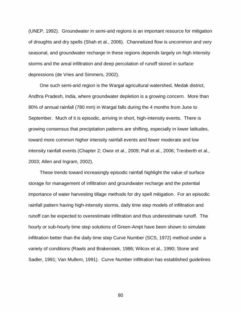
80
(UNEP, 1992). Groundwater in semi-arid regions is an important resource for mitigation
of droughts and dry spells (Shah et al., 2006). Channelized flow is uncommon and very
seasonal, and groundwater recharge in these regions depends largely on high intensity
storms and the areal infiltration and deep percolation of runoff stored in surface
depressions (de Vries and Simmers, 2002).
One such semi-arid region is the Wargal agricultural watershed, Medak district,
Andhra Pradesh, India, where groundwater depletion is a growing concern. More than
80% of annual rainfall (780 mm) in Wargal falls during the 4 months from June to
September. Much of it is episodic, arriving in short, high-intensity events. There is
growing consensus that precipitation patterns are shifting, especially in lower latitudes,
toward more common higher intensity rainfall events and fewer moderate and low
intensity rainfall events (Chapter 2; Owor et al., 2009; Pall et al., 2006; Trenberth et al.,
2003; Allen and Ingram, 2002).
These trends toward increasingly episodic rainfall highlight the value of surface
storage for management of infiltration and groundwater recharge and the potential
importance of water harvesting tillage methods for dry spell mitigation. For an episodic
rainfall pattern having high-intensity storms, daily time step models of infiltration and
runoff can be expected to overestimate infiltration and thus underestimate runoff. The
hourly or sub-hourly time step solutions of Green-Ampt have been shown to simulate
infiltration better than the daily time step Curve Number (SCS, 1972) method under a
variety of conditions (Rawls and Brakensiek, 1986; Wilcox et al., 1990; Stone and
Sadler, 1991; Van Mullem, 1991). Curve Number infiltration has established guidelines

81
for parameterization of tillage management; however, describing tillage for Green-Ampt
infiltration is generally not considered.
Green-Ampt Infiltration and Depression Storage
The Green-Ampt infiltration model (Green and Ampt, 1911) can be described as
an approximate, physically-based model developed from the application of Darcy’s law.
Water is assumed to infiltrate with a distinctly defined wetting front as illustrated in
Figure 3-1. The development of the Green-Ampt equations is a direct application of
Darcy’s Law for deep homogeneous soils with uniform initial water content under
constant, ponded infiltration,
, (3-1)
where q is water flux [L/t], Ks is saturated hydraulic conductivity [L/t], and dH/dz is the
hydraulic head gradient in the direction of flow [L/L]. Adding up heads in Figure 3-1 (dH
= hp + L + ψf), substituting infiltration rate q by dF/dt, where we call F cumulative
infiltration (F = (θs – θi)*L), replacing Ks with Kse (effective hydraulic conductivity,
accounting for air in the soil matrix of unsaturated soils), and substituting the soil
moisture deficit, M, for θs – θi, Darcy’s law then becomes:
or
. (3-2)
Although in reality, 0 < hp(t) < MDS, in the classical use of derivation and use of
the GAML equations, the ponding depth, hp, is assumed negligible and is removed from
the expressions in equation 3-2. Separation of variables and integration results in the
familiar Green-Ampt infiltration equation:
. (3-3)

82
Mein and Larson (1973), Chu (1978) and Skaggs and Khaleel (1982) improved the
applicability of the Green-Ampt equation to allow for calculation under conditions of
variable natural rainfall intensity (with periods of non-ponding and ponding conditions).
The time to ponding, tp, the cumulative infiltration at the time of ponding, Fp, and t’p, the
time to infiltrate Fp if ponding started from the beginning of the rainfall event, were
introduced to allow for the following solution system. For t < tp, f = i (rainfall intensity)
and for t = tp, f = i. Time to ponding can be calculated from tp = Fp/i, where,
. (3-4)
Consideration of the ponding time adjustments finally result into,
. (3-5)
Using this form of the equation, hp appears only in the surface water balance,
calculated after runoff (RO) predicted by GAML, as
dRO = dR – dF – dhp, (3-6)
where dRO [L] is the increment of excess rainfall produced for an incremental rain,
dR [L], dF [L] is the increment in cumulative infiltration for the same time step, and dhp
[L] is the change in surface storage depth for the same period. Equations 3-4, 3-5, and
3-6 will be called the “standard GAML solution” herein. This form of the Green-Ampt
infiltration model now allows for infiltration to be simulated before and after ponding and
if ponding ends and begins again. The MDS=0 solution, shown in the results to illustrate
tillage and MDS importance, represents a negligible hp both as a head and in a surface
water balance. This solution form (MDS=0) is used to predict infiltration and runoff in a
variety of field-scale and landscape-scale hydrologic models, Soil and Water

83
Assessment Tool (SWAT, Arnold et al., 1998; Gassman et al., 2007; Krysanova and
Arnold, 2008) is one example.
It is proposed here that for agricultural systems under some form of water
harvesting tillage, surface storage hp, should be included as a time varying head (0 <
hp(t) < MDS) in the GAML equations in addition to the water balance at the surface (eq.
3-6). To simplify the handling of the time-dependent boundary condition in equation (3-
2) we can assume that hp is constant within each time step but changed for each time
step ( . This simplification is acceptable in water harvesting tillage systems where
dhp for each dt is small relative to the total MDS if the time step is kept sufficiently small.
This allows integration of equation (2) to yield,
. (3-7)
Equations 3-4, 3-6, and 3-7, solved concurrently for each time step will here be
called the “complete GAML solution”. The proposed use of the complete GAML solution
for water conservation tillage systems against the standard formulation is examined by
repeating local and global sensitivity analyses with both forms of the GAML equations:
with hp only included in surface water balance for the conventional Green-Ampt method
(standard GAML) and with hp as a time-varying head in the GAML equation and also in
the surface water balance (complete GAML). Sensitivity analyses were used to
measure the strength of influence of hp on infiltration predictions and to compare GAML
infiltration sensitivity to all the remaining parameters.
Groundwater Recharge and Tillage Management: Modeling Implications
In this chapter, the focus is on improving the performance of infiltration predictions
from the GAML equations through the addition of the typically neglected surface storage

84
depth term, hp; the importance of all five GAML parameters under conventional and
tied-ridge tillage is compared. Conventional tillage describes disking, harrowing,
moldboard plowing, or chisel plowing with no consistent orientation to elevation
contours. Water harvesting tillage is a type of conservation tillage characterized by
significant increases in microrelief or depression storage through the creation of surface
geometries allowing for substantial water storage (i.e. tied-ridge tillage, pit tillage,
contour bunding). Essentially, small basins are formed in croplands which can store
excess rainfall and increase infiltration. The agronomic benefits of water harvesting
tillage are generally realized in the form of increased crop yields resulting from
increased plant available water (Twomlow and Breneau, 2000; Wiyo, 2000; Guzha,
2004; Tesfahunegn and Wortmann, 2008). In addition, increased infiltration can result
in the potential hydrologic benefit of increased groundwater recharge (Foster and
Chilton, 2003), an important benefit in many intensive agricultural areas of the world
where aquifer levels are decreasing (Konikow and Kendy, 2005).
Rainfed agricultural systems, especially those in resource-poor and generally
ungauged watersheds, are increasingly using water harvesting tillage to increase
infiltration depths (Twomlow and Breneau, 2000; Wiyo et al., 2000; Tesfahunegn and
Wortmann, 2008; Derib et al., 2009; Araya and Stroosnijder, 2010), and it may be in
these systems, especially in the tropical regions having vulnerable soils, that alternative
tillage management is the most economical means of increasing production
(Rockström, 2001). Also, irrigated rice croplands, having substantial and well-identified
surface storage depths, are extensive in many typically ungauged watersheds of
Southeast Asia. Including surface storage depth in models using GAML-predicted

85
infiltration is suggested as a possible means of improving model process descriptions
for predictions in ungauged basins (i.e. PUB project, see Sivapalan et al., 2003).
In addition to the growing use of water harvesting tillage in rainfed systems, there
is evidence in the scientific literature and in recent agricultural applications that there is
renewed interest in water harvesting tillage even in humid, irrigated areas (Truman and
Nuti, 2009 and 2010). In Mississippi, USA, for example, water harvesting tillage in the
form of furrow diking (synonymous with tied-ridging) has been approved for cost sharing
under the state’s EQIP (Environmental Quality Incentives Program); for growers
implementing furrow diking, half of the costs are paid by the state. In an analysis of the
hydrology and economics of water harvesting tillage for irrigated cotton in Georgia,
USA, it was found that a grower would recover investment costs for furrow diking tillage
after the first 16 ha-mm of irrigation water savings. This was based on a cost of $1.17 /
ha-mm to pump irrigation water and $18.50 / ha for implementing furrow diking (Truman
and Nuti, 2009). Additionally, furrow diking resulted in a 2.6 times reduction in soil loss
and 25% lower runoff compared to conventional tillage.
There are numerous process-based hydrology and water quality models using
GAML infiltration with fixed or negligible MDS used in a surface water balance and
assuming negligible hp in GAML equations (MDS=0 or standard GAML solution form):
SWMM (Storm Water Management Model; Huber and Dickinson, 1992), PRZM
(Pesticide Root Zone Model; Carsel et al., 1998), WEPP (Water Erosion Prediction
Project; Laflen et al., 1997), SWAT (Soil and Water Assessment Tool; Arnold et al.,
1998), VFSMOD (Vegetative Filter Strip Modeling System, Muñoz-Carpena et al.,
1999), WaSiM-ETH (Water Flow and Balance Simulation Model; Schulla and Jasper,

86
2000), and others. It is argued here that using the complete GAML form in models
using the Green-Ampt method for infiltration prediction, there is no real loss of model
parsimony. If MDS values for various tillage management can be assumed to have less
uncertainty than other infiltration parameters, a reasonable assumption given the
simplicity of measurement, the lower range of values, and the strength of literature
values of MDS (Kamphorst et al., 2000; Planchon et al., 2002; Jones and Baumhardt,
2003; Guzha, 2004), then there may be a reduction in model equifinality concerns,
meaning that a model user may have a better chance of getting the right answer for the
right reasons (Beven, 2006; Gupta et al., 2008; Hughes, 2010).
Parameter estimation completed during GAML model calibration to match
observed data can produce models of similar performance regardless of the solution
form being used. For example in a watershed having extensive areas under water
harvesting tillage, even if the MDS=0 GAML solution is used, streamflow could still be
predicted well after calibration by increasing the values for Kse and/or ψf to achieve the
same runoff reductions that actually result from the MDS of the areas under water
harvesting tillage. The use of additional measured input factors (as opposed to simply
using calibration procedures) is suggested as a way to avoid this problem (Ritter et al.,
2003).
Here it is proposed that including hp (and MDS) in the GAML equations and in a
surface water balance would provide more certain predictions of infiltration and runoff,
compared to MDS=0 and standard GAML solutions, for evaluating hydrologic effects of
water harvesting tillage. The objectives of this chapter were to evaluate the importance
of surface storage depth for Green-Ampt predicted infiltration in agricultural systems

87
under conventional and water harvesting tillage, and to test the proposal that for
systems with water harvesting tillage the surface storage depth could be used to
improve the process description of GAML infiltration.
Methods for Analyzing the Importance of Surface Storage Depth
Site Description
The study area is a 512 ha watershed, called Wargal, in a rural, agricultural region
of northwestern Andhra Pradesh, India (Figure 1-1). Soils in the area are mostly sandy
loam and sandy clay loam with some small areas of clay loam and sandy clay (Soil
Survey Staff, 1999). Rice, maize, cotton, potato, and sunflower are the most commonly
grown crops. Conventional tillage, the typical practice in the area, is either moldboard
or chisel plough drawn by animals and sometimes tractors. Tied-ridge tillage, also
called furrow diking, basin tillage, or reservoir tillage, is the practice of creating earthen
ridges perpendicular to direction of primary tillage (Figure 3-2). Tied-ridging was
selected as the example of water harvesting tillage because it is sometimes used for
potato and other vegetable crops planted late in the rainy season, and equipment is
commercially available for mechanization. The ridges and ties can be created with
hand tools or with a variety of animal-drawn or tractor-drawn implements. Typically,
furrow spacing is 75 to 100 cm with ties every 2 to 6 meters (Jones and Baumhardt,
2003). Ridge and tie heights are approximately 20 cm. Analysis of the surface
geometry suggests a maximum depression storage of 100 mm. Profile measurements
of tied-ridge tilled systems show 50 to 60 mm maximum depression storage (Jones and
Clark, 1987).
Groundwater depletion is a growing concern in the study region as a result of
substantial rice cropland areas, high irrigation withdrawals, density of borewells, and

88
unmetered electrical supply. This is a common scenario in much of India (Rodell et al.,
2009). The broad goal of work in the Wargal watershed is to evaluate combinations of
agricultural management options for improving groundwater recharge and reducing
irrigation withdrawals. These evaluations are being made using a simulated water
balance from the semi-distributed hydrology model, SWAT (Arnold et al., 1998;
Gassman et al., 2007; Krysanova and Arnold, 2008). One of the management options
being investigated for increasing groundwater recharge is to expand the extent of
cropland areas under water harvesting tillage. It is expected that the infiltration
increases from water harvesting tillage would result in groundwater recharge
improvements.
Local Sensitivity Analysis
A simple, local sensitivity analysis (LSA), changing one parameter at a time, was
completed to find the changes in runoff (RO) and infiltration (F) depths obtained for a 4-
hour design storm of 2-year return period in the Wargal area; results from all 3 GAML
solution forms were compared (MDS=0, standard, and complete). Percent changes in F
and RO were calculated based on the difference in RO and F from solutions using
mean MDS for each tillage treatment, conventional (CT) and tied-ridge (TR). Here, only
MDS was varied from its minimum, mean, and maximum values. The purpose of the
local sensitivity analysis was to give a simple, easily interpretable measure of MDS
importance in GAML solutions.
Global Sensitivity Analysis
A global analysis of sensitivity (GSA) was included here to provide a more
complete examination of the importance of MDS in the context of all the GAML
parameters. Additional summaries of GSA methods (Saltelli et al., 2000; Saltelli, 2005;

89
Saltelli et al., 2008) and recent applications to hydro-ecological models (Muñoz-
Carpena et al., 2007; 2010; Muñoz-Carpena and Muller, 2009; Fox et al., 2010; Chu-
Agor et al., 2011) are available.
For a given model input factor Xi, the first-order variance-based global sensitivity
index Si gives the ratio of the output variance if the true value of the input was known to
the total output variance (Y). Formally, a first-order Si is defined as Si = V[ E(Y|Xi) ] /
V(Y), where Xi is a parameter or input of a model, Y is the output of interest, E is
expected value, and V is variance. If a model if perfectly additive, meaning there are no
parameter interactions, then the sum of all Si’s equals 1. This in practice represents a
quantitative measure of how much of the total output variance is explained by the
variation of the single parameter Xi alone (direct effect). First order indexes are used to
select the input factor(s) of the model that would result in the greatest reduction in
variance, V(Y), if the true value of the factor was known; hence they are typically used
to prioritize the importance of model inputs (Saltelli, 2005).
Total-effect global sensitivity indexes, STi are calculated to account for the
presence of interactions (higher order effects). STi gives the ratio of – the expected
amount of variance that would remain if all other input factors were known (fixed) and
only the input factor of interest was varied over its range – to the total output variance
(Y), i.e. STi = E[ V(Y|X-i) ] / V(Y), and are computed similarly to first-order Si. They are
generally used to fix a factor having little influence on V(Y) or to exclude unimportant
input factors during model development (Saltelli, 2005). If a model is non-additive,
meaning there are parameter interactions, then the sum of all STi is greater than 1.

90
A program was developed in Matlab (Mathworks Inc., Natick, MA) for Green-Ampt
infiltration of unsteady rainfall and was used to read in rainfall intensities, GAML
parameters, and solve for cumulative infiltration (F), surface runoff (RO), surface
storage (hpi), and f (infiltration rate). Equation 7, an implicit function in terms of F, was
solved for F using a combination of bisection, secant, and inverse quadratic
interpolation methods (fzero routine in Matlab). hpi was calculated at each time step i
based on rainfall intensity, infiltration rate, previous time step hp-1, and MDS. Variance-
based first-order sensitivity indexes (Si) were obtained for all the GAML parameters for
various storm durations and return periods using the extended Fourier amplitude
sensitivity test (FAST) (Saltelli et al., 1999). These were computed for target outputs
total storm RO and F using the GAML Matlab program linked to the sensitivity and
uncertainty analysis package SimLab 2.2 (Saltelli, 2005) that was used to sample input
parameter sets and for post-processing of outputs to generate sensitivity indexes.
Parameter sets of size 5000 were generated from the ranges and probability
distributions selected for all five Green-Ampt parameters.
Parameters for Green-Ampt Infiltration Sensitivity Analysis
The first step in a good sensitivity analysis is a clear understanding of the
objective; here, the first objective of the sensitivity analysis was to rank the relative
importance of surface storage depth against all other model input factors for two tillage
strategies: conventional (CT) and tied-ridge (TR). The second step is to develop ranges
and probability distributions for all parameters of the model being used. Table 3-1
displays parameter values needed to use the Green-Ampt model for unsteady rainfall at
the Wargal site. Ranges of the Green-Ampt parameters for the study area were based

91
on observations and estimations from literature values; probability distributions were
assigned to each of the parameters based on the range and values found.
Laboratory measurements of saturated hydraulic conductivity were performed on
undisturbed soil cores collected from the experimental site (Figure 1-1) by partners at
Acharya N. G. Ranga Agricultural University (ANGRAU) in variable depth increments
from 0 – 1 m (136 samples from N = 37 locations); there were typically samples from 4
soil layers at each location. Values of saturated hydraulic conductivity (Ks) ranged from
0.131 to 165 mm/hr, based on constant head permeameter Ks measurements. For use
in Green-Ampt, Ks values only in the top soil layer (0 – 30 cm) were used; the geometric
mean Ks in this layer was 31.8 mm/hour. Hydraulic conductivity (K) of soil is dependent
on water content; generally a drier soil has a lower K than a wetter soil. The effective
hydraulic conductivity (Kse) in the Green-Ampt equation accounts for this air entrapment
making Kse < Ks. The recommendation of Bouwer (1966) is to approximate Kse using
Kse = 0.5*Ks; this approximation was used here in the absence of field measurements of
Kse. A log-normal probability distribution was fitted to the Kse data; Weibull, log-normal,
and Generalized Extreme Value (GEV) distributions were compared graphically. The
GEV distribution fit the data most closely, but the log-normal distribution, also a good fit,
was selected because it is what is typically used for Ks distribution (Carsel and Parish,
1988; Meyer et al., 1997) and the GEV distribution is unavailable in the SimLab (Saltelli,
2005) sensitivity/uncertainty analysis package that was used here.
There were no observations of average wetting front suction average (ψf) values
for soils in Wargal watershed. The soil properties tables of Rawls et al. (1983) were
used to estimate ψf based on observed soil texture data. The soil texture used here

92
was sandy loam; it was one of the two dominant textures based on observations and
measured Ks values were more consistent with those associated with sandy loam than
with sandy clay loam. Soil texture analysis for the experiment site was made using the
Bouycous Hydrometer method (Kalra and Maynard, 1991). Without additional data for
determination of a probability distribution, the distribution of ψf was assumed uniform
with parameters given in Table 3-1.
The initial volumetric water content (θi) and saturated volumetric water content (θs)
were obtained like ψf using tabular data for sandy loam soil (Rawls et al., 1983;
Fangmeier et al., 2005). Spatial variability is typically high for these parameters and
temporal variability is high for θi. Literature values based on soil texture were the best
estimates available for the study area.
The maximum surface storage depth (MDS) represents the maximum depth of
surface storage of water over an area. It is the equivalent depth of water stored on the
surface of the entire area if it was covered with an equal depth of water everywhere.
There is not sufficient data in the literature to recommend changes in the other
parameters for different tillage. Tillage is expected to influence infiltration through soil
surface geometry changes, not through changes in soil structure. MDS is changed
because significant differences in this parameter have been found for different kinds of
tillage (Table 3-1). Based on a summary of literature values, MDS will be given a mean
value of 5 mm for conventional tillage. With no data about distribution of MDS
measurements, distribution will be assumed uniform: minimum and maximum MDS of 0
and 10 mm, respectively, for conventional tillage. MDS for tied-ridging will be assigned
a mean of 32.5 based on the assumed uniform distribution and using the minimum

93
value of Guzha et al. (2004) of 15 mm depression storage and a maximum value of 50
mm based on a conservative assessment of surface geometry and the work of Jones
and Clark (1987).
Development and Selection of Design Storms for the Analysis
Hourly data of rainfall from 1993-2008 (16 years; Singh, 2009) from recording
gages at the International Crops Research Institute for the Semi-arid Tropics (ICRISAT)
near Hyderabad, Andhra Pradesh, India (20 km from study area) were used to generate
rainfall intensity-duration-frequency (IDF) curves that were used for synthetic storm
generation of design storms. IDF relationships were developed by fitting a probability
distribution function to the annual maximum series rainfall intensity data (separately for
selected durations: 2, 4, 8, and 24 hours). Parameters for distribution functions were
estimated using maximum likelihood estimation. Three distribution functions commonly
used for rainfall IDF representation, Gumbel, Gamma, and Weibull (Koutsoyiannis et al.,
1998; Mohymont et al., 2004), were compared graphically with the empirical cumulative
distribution functions (CDF) of annual maximum series rainfall for the selected
durations.
Results and discussion of GAML Infiltration Sensitivity Analyses
Representative Design Storm for the Analysis
Plotting the Gumbel, Gamma, and Weibull CDF with the empirical CDF of 4-hour
rainfall annual maximums showed similar fit to the data for Weibull and Gamma
distributions (Figure 3-3). The Weibull distribution function was selected to be used
here based on simplicity of form and frequency of use in the literature (Wilks, 1989; D.
Koutsoyiannis et al., 1998; Madsen et al., 2009). The 16 year hourly rainfall record
could be considered too brief for prediction of intensities and durations of low frequency

94
storms (75 and 100 years; Table 3-2), but the unusually heavy rainfall events of August
2000 (92-year daily high rainfall for Hyderabad; Geological Survey of India, 2001) result
in rainfall IDF relationships that can be considered reliable for low frequency storms. As
only 2, 5, and 10 year storms of 4 hour duration were used here, this record was
deemed adequate for generating design storms of those frequencies.
In the 16 year period of record, there were seventy 4-hour storms, thirty-three 6-
hour storms, and nine 8-hour storms; these were analyzed to determine storm type for
the area using mass distribution curves. Analyses of rainfall mass distribution curves
suggest storms should be described as Type II (SCS, 1986), meaning total depths of
rainfall before and after half of the storm duration are about equal, and peak rainfall
intensity occurs at half the storm duration; this is sometimes referred to as an
intermediate storm. The low number of long duration storms for the record period (nine
8-hour storms) is evidence of the episodic nature of rainfall in the region; storms are
typically short and of high intensity. Therefore, it was decided to consider 4-hour
storms for this analysis given that storms of this duration are much more common than
8-hour or 24-hour storms). The rainfall intensity-duration-frequency (IDF) data used to
develop design storms are presented in Table 3-2. The rainfall intensity data for 4-hour
design storms of the three return periods (2, 5, 10-year return period) that were used for
this analysis are presented in Table 3-3.
Tillage and MDS: GAML solution form
The differences in infiltration and runoff depths between the standard and
complete GAML solutions are demonstrated in Figure 3-4. For the MDS range of
conventional tillage (CT; 0-10 mm), there are small differences in predicted RO and F.
On average across the MDS range for CT, using the complete GAML form, predicted F

95
was 1.2% greater and predicted RO was 2.5% lower than the F and RO predicted using
the standard GAML form. These differences increase substantially for the MDS range
of tied-ridge tillage (TR; 15-50 mm). On average across the MDS range for TR, using
the complete GAML form, predicted F was 5.8% greater and predicted RO was 40.8%
lower than the F and RO predicted using the standard GAML form. This shows that the
solution form should be considered for GAML predictions in agricultural areas with
significant MDS (> 15 mm). Also, Figure 3-4 demonstrates the importance of the MDS
parameter for describing tillage, for either GAML solution form. The global sensitivity
analysis was required to make quantitative comparisons between the importance of
MDS and the other 4 GAML parameters.
Local sensitivity analysis
Results of the local sensitivity analysis (LSA; Table 3-4 and Figure 3-5) illustrate
substantial infiltration and runoff depth differences between CT and TR tillage
treatments, meaning that MDS can be an important parameter for improving
descriptions of tillage management. Under the complete GAML solution with mean
MDS values of 32.5 mm and 5.0 mm for tied-ridge (TR) and conventional tillage (CT),
respectively, total runoff depth was 65% lower for TR than for CT, and predicted total
storm infiltration was 31% greater for TR than for CT. Differences in RO and F within
tillage treatments and between solution forms show that the manner in which hp is
included in GAML solutions is important for tillage treatments with significant MDS (> 15
mm). For TR with mean MDS using the complete GAML solution form, predicted RO
decreased by 31% and F increased by 6% compared to the standard GAML form.
GAML solution form is less important in conventionally tilled areas with low MDS (< 10

96
mm): for CT with mean MDS and the complete GAML solution form, predicted RO
decreased by 3% and F increased by 6% compared to the standard GAML form.
Global Sensitivity Analysis
The first-order sensitivity indices (Si) for each of the GAML parameters for both
tillage treatments and both GAML solution forms are reported in Table 3-5 and Figure 3-
6. Design storms of 4-hour duration (T = 2, 5, and 10 years) were used. The Si of
Table 3-5 show that for a tied-ridged system, MDS is the second most important
parameter for GAML-predicted infiltration, meaning that for tillage with non-negligible
surface storage, the parameter MDS is shown to explain more output variability in F and
RO than all other parameters except Kse; parameters ranked by importance are: Kse,
MDS, ψf, θs, θi. Of the five GAML parameters, Kse and MDS are the two parameters
that are the least likely candidates for elimination from the solution or for fixing at a
constant value for uncertainty analysis. Also, differences in Si of MDS between the two
forms of GAML solutions gives more evidence that it does matter how hp is included in
the GAML equations, as indicated by the percent differences in MDS S i between
complete and standard GAML solutions (Table 3-5). Under tied-ridging, using the
standard GAML solution form resulted in decreases in the S i for MDS of around 23%,
making it of importance comparable to ψf, but MDS remained the second most
important parameter using the standard GAML form. For a conventionally tilled system,
sensitivity of infiltration to MDS is expectedly smaller but is still significant and is greater
than that of θs; parameters ranked by importance are: Kse, ψf, θs, MDS, θi. There were
significant changes in MDS Si between solution forms for simulations using CT, but the
lower overall Si of MDS compared to those under TR, mean that the manner in which H
is included in the GAML solution is of little importance for conventionally tilled systems.

97
Plotting Si for the GAML parameters, Figure 3-6 illustrates the strength of influence
of parameters on the variability of the outputs of interest (RO and F). Given the
parameter ranges and distributions for sandy loam soils and tillage systems typical of
this study area, it is evident that MDS becomes a significantly more important parameter
if there is tillage having surface storage ranging from 15-50 mm. However, in systems
having less surface storage (0-10 mm), MDS is one of the least important parameters.
Figure 3-6 suggests that in studies of infiltration and runoff in conventionally tilled
agricultural systems, most efforts should be directed toward improving estimates of Kse
and ψf. It also suggests that in systems employing some type of tillage to reduce runoff,
most efforts should be directed toward improving estimates of Kse and MDS. The sum
of all Si was about 0.98, meaning that the model is almost perfectly additive; therefore,
any refinement to a parameter will result in direct reductions in output uncertainty.
Conclusions on the Importance of Surface Storage Depth for Tillage Parameterization
One outcome of sensitivity analysis is to guide investigators about which uncertain
input factors contribute the most to the model output uncertainty. This study shows that
Kse and MDS are the most important factors controlling total infiltration (F) and runoff
(RO) in systems having tillage with significant depression storage. As a result, the most
attention and resources spent on parameterization of GAML-predicted infiltration should
focus on the parameters to which infiltration is most sensitive.
Substantial differences in predicted runoff and infiltration depths between
conventional (CT) and tied-ridge tilled (TR) systems were observed; therefore, MDS
was shown to be a useful parameter for describing water harvesting tillage. The results
demonstrated here show small differences in F and RO for CT between the two solution

98
forms, standard and complete, suggesting that the typical simplification of GAML to the
standard form is an adequate solution for GAML predictions under conventionally tilled
systems. However, the marked differences in first order variance-based global
sensitivity indexes Si for F and RO depths between the two solutions for TR suggest
that hp should be included both in the water balance and in the Green-Ampt equations.
The main advantage of the complete GAML solution over the MDS=0 and
standard GAML solutions is that it represents a simple way to describe water-harvesting
tillage (using the MDS parameter and the accompanying time-varying hp) and to reduce
the uncertainty of infiltration and runoff predictions. Thus, hydrologic models equipped
with the complete GAML solution could become useful tools for estimating the
landscape-scale impacts of water-harvesting tillage (of different MDS and areal extent)
on infiltration, evapotranspiration, and groundwater recharge.
Based on the predicted infiltration increases from water harvesting tillage and also
on the growing evidence of changing precipitation character, it could be expected that
surface storage of excess rainfall will become an increasingly important management
concern in agricultural areas and that there may be an increase in extent of agricultural
systems having some form of water harvesting tillage, including tied-ridging, contour
bunding, or pit tillage. Therefore, the advantages of the complete GAML solution
demonstrated here could provide improved predictions of infiltration and runoff for field
and landscape-scale hydrologic models employing standard or MDS=0 GAML solutions.

99
Figure 3-1. Illustration of infiltration modeled by Green-Ampt equation. θ, θs, θi, are volumetric water content, saturated and initial, respectively, hp is depth of water ponded at the surface, L is distance from surface to the wetting front, ψf is wetting front suction.
Figure 3-2. Typical furrowed field beside tied-ridged field following rain event (image from Jones and Baumhardt 2003)

100
Table 3-1. Parameter values needed for Green-Ampt model: minimum, maximum, mean values and estimated probability distributions. Initial water content (θi), saturated water content (θs), effective hydraulic conductivity (Kse), wetting front suction (ψf), and maximum depression storage depth (MDS) for conventional tillage (CT) and tied-ridge tillage (TR).
Parameter Min Max Mean Units Distribution
θi 1 0.1 0.2 0.1 mm/mm uniform
θs 1 0.4 0.6 0.5 mm/mm uniform
ψf 1 26.7 194.0 110.4 mm uniform
Ke 2 1.1 44.1 15.9 mm/hr log-normal (μ = 2.23, σ = 1.03)
MDS (CT) 3 0.0 10.0 5.0 mm uniform
MDS (TR) 4 15.0 50.0 32.5 mm uniform 1 Rawls et al., 1983; Fangmeier et al., 2005 2 laboratory analysis of local soils in Wargal study area
3 Kamphorst et al., 2000; Planchon et al., 2002; Guzha et al., 2004 4 Guzha et al., 2004; Jones and Clark, 1987
Figure 3-3. Empirical CDF for annual maximum series (AMS) rainfall intensity for 4 hour storms; Weibull, Gamma, and Gumbel CDF fitted to AMS data using maximum likelihood parameter estimation.
0
0.2
0.4
0.6
0.8
1
0 20 40 60 80 100 120
Cum
ula
tive p
robabili
ty
Annual maximum series rainfall intensity (4 hour storm; mm/hour)
AMS data CDF
Weibull CDF
Gamma CDF
Gumble CDF

101
Table 3-2. IDF data (1993 – 2008 hourly rainfall), Weibull distribution used, values in the table are rainfall intensities in mm/hour
Duration t,(hours)
T, return period (years)
2 5 10 15 25 50 75 100
1 42.3 62.4 73.6 79.3 85.9 94.0 98.3 101.3
2 29.0 45.8 55.5 60.6 66.6 74.0 78.0 80.8
4 17.3 29.3 36.8 40.7 45.4 51.4 54.7 56.9
8 10.0 17.3 21.9 24.3 27.2 30.9 32.9 34.3
24 4.7 8.6 11.2 12.6 14.2 16.4 17.6 18.5
Figure 3-4. Infiltration (F) and runoff (RO) for a 4-hour 2 year design storm; complete and standard GAML solutions
0
20
40
60
80
100
120
140
160
180
0 5 10 15 20 25 30 35 40 45 50
F, R
O d
epth
s (
mm
)
MDS (mm)
F, complete GAML
F, standard GAML
RO, complete GAML
RO, standard GAML
CT TR

102
Table 3-3. 4-hour design storms of 2, 5, 10-year return period used for rainfall input in GAML sensitivity analysis; 20 min time step
Duration Design storm intensity, mm/hr
hours 2 year 5 year 10 year
0.00 0.0 0.0 0.0
0.33 24.8 29.8 34.2
0.67 27.2 32.7 37.6
1.00 30.5 36.7 42.2
1.33 35.5 42.6 49.0
1.67 43.7 52.6 60.4
2.00 62.6 75.3 86.5
2.33 89.6 107.7 123.8
2.67 50.8 61.0 70.1
3.00 39.0 46.8 53.8
3.33 32.7 39.3 45.2
3.67 28.7 34.5 39.7
4.00 25.9 31.1 35.8
Table 3-4. GAML predicted runoff (RO) and infiltration (F) depths of conventional (CT) and tied-ridge (TR) tillage for 2 year, 4-hour storm; standard and complete GAML solutions. Min, mean, and max MDS were 0, 5, 10 mm for CT and 15, 32.5, 50 mm for TR.
Runoff Infiltration Complete GAML solution
MDS TR CT MDS = 0 TR CT MDS = 0
Min 40.7 59.7 59.7 123.0 104.0 104.0
Mean 18.9 53.3 59.7 144.8 110.3 104.0
Max 0.0 47.0 59.7 163.7 116.7 104.0
Runoff Infiltration Standard GAML solution
MDS TR CT MDS = 0 TR CT MDS = 0
Min 44.7 59.7 59.7 119.0 104.0 104.0
Mean 27.2 54.7 59.7 136.5 109.0 104.0
Max 9.7 49.7 59.7 154.0 114.0 104.0

103
Figure 3-5. Infiltration and runoff % changes from mean MDS values for 2 year, 4-hour storm for both GAML solution types; min, mean, max are values of MDS for conventional (CT: 0, 5, 10 mm) and tied-ridge (TR: 15, 32.5, 50 mm) tillage.
-15
-10
-5
0
5
10
15
min mean max
% C
hange in infiltra
tion f
rom
mean M
DS
infiltra
tion
CT: complete GAML
TR: complete GAML
CT: standard GAML
TR: standard GAML
-150
-100
-50
0
50
100
150
min mean max
% C
hange in r
unoff f
rom
mean M
DS
infiltra
tion
CT: complete GAML
TR: complete GAML
CT: standard GAML
TR: standard GAML

104
Table 3-5. First order sensitivity indexes (Si) for output F of the 5 GAML parameters for tied-ridge (TR) and conventional tillage (CT) for both GAML solution forms, complete and standard.
Tillage type Si of GAML parameters solution form Kse ψf θs θi MDS storm t, T %change
TR 0.8210 0.0343 0.0117 0.0069 0.1105 4 hour, 2 year complete 0.8384 0.0358 0.0115 0.0062 0.0891 4 hour, 5 year GAML 0.8425 0.0375 0.0131 0.0062 0.0815 4 hour, 10 year
TR 0.8273 0.0578 0.0099 0.0053 0.0858 4 hour, 2 year 28.8%
standard 0.8378 0.0571 0.0091 0.0048 0.0685 4 hour, 5 year 30.1%
GAML 0.8390 0.0588 0.0106 0.0049 0.0623 4 hour, 10 year 30.8%
CT 0.8982 0.0588 0.0115 0.0063 0.0115 4 hour, 2 year complete 0.8951 0.0573 0.0106 0.0055 0.0089 4 hour, 5 year GAML 0.8925 0.0581 0.0118 0.0054 0.0081 4 hour, 10 year
CT 0.8965 0.0641 0.0110 0.0060 0.0079 4 hour, 2 year 45.6%
Standard 0.8934 0.0620 0.0101 0.0053 0.0059 4 hour, 5 year 50.8%
GAML 0.8905 0.0627 0.0113 0.0052 0.0054 4 hour, 10 year 50.0% 1 % change in MDS Si is the increase in MDS Si when changing from standard to complete GAML solution
form

105
Figure 3-6. Total effect sensitivity indices (outputs are F and RO; their sensitivities to each parameter are equal) for Green-Ampt parameters for tied-ridge and conventional tillage for 4 hour design storm of 2 year return period.
0
0.2
0.4
0.6
0.8
1F
irst ord
er
sensitiv
ity indic
es
TR: complete GAML
TR: standard GAML
CT: complete GAML
CT: standard GAML
Kse ψf θs θi MDS

106
CHAPTER 4 EVALUATION OF AGRICULTURAL MANAGEMENT ALTERNATIVES FOR
SUSTAINABLE GROUNDWATER IN INDIA: SIMULATED WATER BALANCE RESULTS
Overview of Water Balance Simulation
Groundwater Management in India
There are 170 Mha of cultivated land in India – more than half the total land area
of 328 Mha (FAOSTAT, 2010). Irrigated areas are 45% (77 Mha) of total cultivated area
(AQUASTAT, 2010), and more than half of the irrigation requirements are from
groundwater resources (CGWB, 2002; Shah et al., 2003). Total groundwater
withdrawals of 251 billion km3 are the highest of any nation (AQUASTAT, 2010). The
harvested area of rice croplands in India (44 Mha) and the irrigation diversions for rice
areas are greater than those of all other crops, and rice production at the national scale
is the most valuable agricultural activity – valued at $30 billion/year (FAOSTAT, 2010).
Field-scale water balance experiments in the Wargal study area have shown a
groundwater balance of about -690 mm (1235 mm or irrigation; 542 mm of return flow
recharge) for a rainy-season rice cropping system (Reddy, 2009). All these data should
lead to the conclusion: rice cropland areas in India are extensive, highly important
economically, have large consumptive water use, and depend heavily on groundwater
resources.
For farming households, which make up about half of the population of India
(FAOSTAT, 2010; 2009 population of India), groundwater depletion is concerning
because it is expensive and increases vulnerability. A study of the costs of groundwater
depletion in Andhra Pradesh has shown that increasing groundwater recharge is the
most economical way to manage groundwater depletion (Reddy, 2005). The water

107
balance simulations of this research in the Wargal watershed have served to quantify
the impacts on the groundwater balance of recharge structures (small reservoirs),
current farm management practices, and alternative farm management options. The
costs of groundwater depletion refer to capital losses resulting from borewell
infrastructure being ineffective due to lower groundwater levels, new required
investments to deepen borewells and lower pumps, higher energy costs for
groundwater withdrawal, and the indirect costs of lower net incomes from reduced areas
of flooded rice croplands. It was shown in the study by Reddy (2005) of three villages in
northern Andhra Pradesh that groundwater depletion costs are most damaging to
farmers with smaller land holdings, and disparities in groundwater access and control
generally develop – those having larger land holdings are able to adapt to groundwater
depletion and retain access to groundwater resources.
The options for managing groundwater depletion are numerous, but they can be
simplified into the following categories: increasing surface storage and infiltration of
excess rainfall (to increase groundwater recharge), reducing groundwater withdrawals,
and decreasing evapotranspiration (ET) in rainfed and irrigated croplands. This is
explained in the conceptual model and discussion of surface and groundwater balances
in Chapter 1. The simulated water balance experiments presented in this chapter serve
to examine some of the possible agricultural management options for groundwater
sustainability; the best options for groundwater sustainability are evaluated based on
predictions of groundwater recharge and withdrawals, ET, and estimated household
incomes.

108
Goals of Simulated Water Balance Experiments
In consideration of the significance of groundwater resources in India, there are
three hypotheses being tested in this chapter by simulating the water balance of the
Wargal watershed: (1) current rice cropland extent and management practices are
depleting groundwater supplies, (2) tillage for water harvesting can significantly increase
groundwater recharge in rainfed croplands, and (3) there are combinations of tillage,
crop selection, and irrigation that can improve groundwater recharge and reduce
groundwater withdrawals. The objectives of the simulation experiments:
Assess groundwater sustainability of agricultural management practices (crop selection, irrigation management, tillage) at a watershed scale – quantify the groundwater balance (recharge – irrigation pumping) under current and alternative agricultural management
Evaluate improvements to the Green-Ampt infiltration routines of a hydrologic model (Soil and Water Assessment Tool – SWAT; Arnold et al., 1998; Krysanova and Arnold, 2008) for simulating groundwater balance under various cropping systems
Water Balance Simulation Methods
SWAT Preparation
Preparing SWAT for hydrologic simulations required spatial datasets for soils,
topography, climate, and LULC as described in Chapter 1: “Summary of Water Balance
Simulation Methods.” Detailed management of agricultural areas was described using
planting dates, harvest dates, and irrigation information based on data from the Wargal
area. Code modifications were made (Appendix A) to accommodate a surface storage
depth for parameterization of water harvesting tillage. Agricultural management
alternatives were prepared by developing text files to change cropland areas, irrigation
depths, and tillage-induced MDS.

109
Describing agricultural management
Dates for planting and harvesting were those typical of kharif (June-September,
rainy season), rabi (October-February), and summer seasons (March-May).
Flowmeters on borewells were used to estimate daily irrigation applications for rice in
kharif (N = 6, where N is the number of seasonal flowmeter records) and rabi (N = 5)
seasons and for vegetables in summer (N = 4). Flow volumes were monitored by
research partners from ANGRAU, measured field sizes allowed for conversion to
application depth. Based on flowmeter data, daily irrigation applications in kharif and
rabi seasons for rice were 8 mm/day and were 4 mm/day for vegetables in summer
season. Modeling cropping system sequences (in kharif, rabi, and summer) required
adjusting cropland areas dynamically 3 times each year. This was accomplished in
SWAT using a lup.dat (land-use update) file and 3 text files which described changing
cropland areas that were read-in by SWAT at specified dates each year. The seasonal
cropland area files and lup.dat were also used for describing changed cropland areas
for alternative management options.
To compare the water balance results of alternative agricultural management,
existing management and 25 alternative management scenarios were simulated (Table
4-1) both for observed weather data (2009-2010) and for a 10-year simulation using
generated weather data (2000-2009) from WXGEN (Sharpley and Williams, 1990)
included in SWAT. WXGEN weather data were generated based on a database of 168
climate parameters for the Wargal watershed. Simulations were completed for both
measured and generated weather data because the years of 2009 and 2010, for which
there are observations of weather data, are not necessarily good representations of
average annual rainfall. In 2009, annual rainfall was 667 mm (about 110 mm below

110
normal); in 2010, annual rainfall was 1022 mm (about 240 mm above normal). The use
of simulated weather data also resulted in some dry and some wet years, but the
average annual rainfall during the 10 years (792 mm) was very close to the long term
average in Wargal of 780 mm. Most of the results presented are from the 2000-2009
generated weather dataset because it was decided that the rainfall data of the
generated dataset better represented average conditions. The trends in results were
nearly identical for both weather datasets.
SWAT process modifications
To test the significance of tillage management for increasing groundwater
recharge the GAML infiltration routines of SWAT were modified to allow for
parameterization of tillage using a maximum depression storage (MDS) value – see
Chapter 3 “Green-Ampt Infiltration and Depression Storage” and Equation 3-2. In order
for the modified infiltration routine to work properly, 22 subroutines of SWAT required
alterations (Appendix A). The subroutines requiring the most extensive changes were
those for GAML infiltration (surqgreenampt.f), actual evapotranspiration (etact.f),
irrigation from aquifer (irrsub.f), and tillage description (newtillmix.f and readtill.f). The
infiltration routine was altered to allow for accumulation of surface storage of excess
rainfall which created a time-varying head that influenced infiltration rates (Chapter 3).
After modifications, surface storage accumulated up to the MDS value; additional
excess rainfall became surface runoff. ET routine changes were made in order for
stored surface water in cropland areas to be evaporated; evaporation rates were
dependent on leaf area index as modeled by SWAT. The irrigation routine was
changed so that irrigation applications could be stored on the surface if they were in
excess of infiltration rates and there was a non-zero MDS value. The tillage description

111
routines were changed to add the MDS parameter to the till.dat tillage database and to
create the correct MDS in an area after a tillage operation with non-zero MDS was
completed. These changes have allowed for ponded rice to be simulated more
accurately and in combination with dynamically varying cropland areas; this was not
possible with previous releases of SWAT.
SWAT Calibration and Evaluation
Model calibration is the estimation of parameters of model to improve its
predictions of observed data. Model evaluation is the quantitative assessment of the
performance of a model in predicting observations which were not used for model
development or parameter estimation (calibration). The target for SWAT calibration and
evaluation was a time series of 50 reservoir volumes from 3/19/2010 to 12/3/2010
(Figure 4-1); this was the best available runoff gauge given that there is limited
channelized flow in the watershed. The reservoir at the outlet of the Wargal watershed
creates a generally closed watershed, and the volume of water stored in this reservoir
was considered a good substitute for streamflow data which are typically used to
calibrate and evaluate hydrologic models. This time series of reservoir volumes begins
in a dry portion of the year and extends beyond the rainy kharif season. As discussed
in Chapter 1, these observations were obtained from GPS waypoint data and tank level
gage data to measure flooded area and depth of water, respectively.
The 13 most important parameters of SWAT were varied across a specified range
based on field data and literature values. Varying these 13 parameters required re-
writing 838 text files for input to SWAT; therefore, automated calibration software was
required. SWAT-CUP3 (Abbaspour, 2008), a program developed by the systems
analysis and modeling group of Eawag (Swiss Federal Institute of Aquatic Science and

112
Technology), was used for SWAT calibration, evaluation, and sensitivity and uncertainty
analysis. Generalized likelihood uncertainty estimation (GLUE) was implemented
(Beven and Binley, 1992) in SWAT-CUP3. GLUE requires few assumptions about
parameter distributions and is a simple model-independent method for parameter
estimation. GLUE allows for the non-uniqueness of model realizations, meaning that
numerous parameter sets can result in a model having similar performance. Model
uncertainty comes only from parameter uncertainty under GLUE methodology. There is
flexibility in the choice of performance measure or objective function. Here the Nash-
Sutcliffe efficiency (NSE) was used; it is one of the 3 quantitative model evaluation
techniques recommended in the model evaluation guidelines work of Moriasi et al.
(2007). NSE is expressed by:
NSE =
(4-1)
where Yiobs is the i-th observation for the output of interest, Yi
sim is i-th simulated value,
and Ymean is the mean of all the observations used (n total observations). The range of
NSE is - ∞ to the optimal value of 1. NSE > 0.5 is said to describe satisfactory model
performance (Moriasi et al., 2007).
Model evaluation was by graphical comparison, NSE, percent bias (PBIAS), and
the root mean squared error (RMSE) observations standard deviation ratio (RSR) were
the 4 methods used to evaluate model performance, following the recommendations of
Moriasi et al. (2007). PBIAS and RSR are expressed by:
PBIAS =
(4-2)

113
RSR =
(4-3)
NSE > 0.5, RSR < 0.70, and PBIAS < |25%| can be said to describe satisfactory model
performance (Moriasi et al., 2007) for monthly data of streamflow. These guidelines
should of course be adjusted based on prediction variable (sediment, phosphorus, or
others), observation time step, and measurement uncertainty (Moriasi et al., 2007).
These guidelines are generally more stringent for streamflow predictions than for other
variables (water quality) and model performance is usually worse as observation time
step is reduced (Engel et al., 2007; Yuan et al., 2001); that is, model performance on a
monthly basis can be expected to be greater than that on a weekly or daily basis. The
average observation time step of the reservoir volumes used for model calibration and
evaluation in the Wargal watershed was 5 days (range of 1 to 28 days).
There was one year of reservoir volumes available for use for model calibration
and evaluation; therefore, some strategy was required to be able to use all the data for
both model evaluation and calibration. K-fold cross-validation is one strategy that
allows all the data to be used for parameter estimation and for model evaluation
(Wallach et al., 2006). Cross-validation is similar to the method of splitting a dataset
into 2 parts and using one part for parameter estimation and one part for evaluation of
the model. In cross-validation, an observation or group of observations is removed from
the dataset and parameter estimation proceeds. Since the observations removed were
not used for parameter estimation, the model can be safely evaluated for its ability to
simulate the removed observations. Next, the observation or group of observations is
replaced, and the next observation or group of observations is removed and the model

114
calibrated again. This continues until all data have been removed and replaced. In the
Wargal area, groups of 10 observations from the record of 50 were removed, meaning
5-fold cross-validation was used. The result is 5 different estimates of the parameter
vector which are each used separately to predict the reservoir volume to evaluate the
model. One of the advantages of cross-validation is that all the data are used in the
same way for both model calibration and evaluation (Wallach et al., 2006).
Deciding which parameters to vary (and by how much) is an important part of
model calibration. The literature on calibration of SWAT was used to assist with choices
of parameters for calibration (Bosch et al., 2004; Van Liew et al., 2005 and 2007). A
departure from typical practice was that saturated hydraulic conductivity (Ks) for soils
was varied separately for rice croplands and other areas due to the uniquely low Ks of
puddled rice soils. Puddling describes the tillage of rice fields when they are flooded;
the resulting particle settling in order of particle size (largest to smallest) results in a soil
of very low hydraulic conductivity (Kukal and Aggarwal, 2002; Marechal et al., 2006).
More than 15 GLUE calibration/sensitivity runs (each of N=5000 or N=2500) were
completed using anywhere from 5 to 14 parameters for calibration; these preliminary
calibration efforts were used to decide on the final 13 parameters to calibrate and how
much they should vary. Parameter ranges were carefully selected (based on
observations in Wargal and literature values) to ensure values did not depart from
realistic ranges for the soils and land use of Wargal.
Parameter sensitivity and uncertainty analysis
A complete, global sensitivity analysis of SWAT is not an objective of this work;
this has been done well by others (van Greinsven et al., 2006), but it is important to
have a meaningful ranking of parameters by order of importance. A sensitivity analysis

115
was completed through SWAT-CUP3 to determine parameter sensitivities using the
multiple regression system: (Muleta and Nicklow, 2006; Abbaspour et
al., 2007). This system regresses the Monte Carlo sampled parameters from GLUE
against the predicted reservoir volumes, g. A t-test and accompanying p-value are used
to compare the relative sensitivities of each parameter bi; p-value is the probability that
the absolute value of the regression coefficient βi would be as large or larger if there
was no relationship between that parameter bi and the output, g (Helton and Davis,
2000). A low p-value corresponds to an important parameter (low probability of the
parameter not making significant changes to predicted reservoir volume). The
sensitivities calculated are based on linear approximations of the sensitivity of the model
output to changes in a parameter while all other parameters are changing; therefore, it
is a type of global sensitivity (Muleta and Nicklow, 2006); this method requires a large
number of simulations and is dependent on choice of parameter ranges (Abbasour et
al., 2007).
SWAT-CUP3 (Abbaspour, 2008) uses a flexible format to assist with generation of
parameter sets for calibration and model sensitivity analysis. The following system
defines the range of a parameter:
x__<parname>.<ext>__<hydrogrp>__<soltext>__<landuse>__<subbsn>__<slope>. X
is the type of change applied to the parameter (x = v, a, or r): v__ means the original
parameter value is to be replaced by a value in the specified range, a__ means a value
from the specified range is added to the original parameter value, and r__ means the
original parameter value is multiplied by (1+ a value in the specified range). <parname>
is the SWAT parameter name, <ext> is the SWAT file extension, <hydrogrp> is the soil

116
hydrologic group (A, B, C, D; optional), <soltext> is the soil texture (optional), <landuse>
is the landuse category (in this study it is just crop type, optional), <subbasin> is the
number of the subbasin in the watershed (in this study it is 1 to 6, optional), and <slope>
is the class of slope range (optional). The 13 parameters varied for sensitivity and
uncertainty analyses were, in order of importance based on the step-wise regression-
based global sensitivity analysis described earlier:
SOL_AWC(layer#): available water holding capacity of the soil layer in mm water / mm soil. This was varied in soil layers 1 and 2 for Wargal.
SOL_K(layer#): saturated hydraulic conductivity of the soil layer in mm/hr. This is actually 2 parameters as this was adjusted separately in layer 1 of rice croplands.
RES_K: hydraulic conductivity (mm/hr) of a reservoir bottom.
CN2: the initial SCS curve number for moisture condition II; it is a function of soil permeability, land use, operations, and soil moisture.
EVRSV: reservoir evaporation coefficient (0-1) used to adjust for shading and vegetation cover.
GWQMN: the threshold depth of water (mm) in the shallow aquifer required for baseflow to occur.
EPCO: plant water uptake compensation factor; this is another calibration parameter similar to ESCO. EPCO ranges from 0.01 to 1, and the closer to 1 EPCO is the more plant water uptake is allowed to come from deeper soil layers.
ESCO: soil evaporation compensation factor; this is a calibration parameter that adjusts the depth in the soil profile from which evaporation can occur. ESCO ranges from 0.01 to 1, and values closer to 1 increase the depth at which evaporation from soil can occur.
ALPHA_BF: is an index of the groundwater flow response to recharge changes; it is close to 1 for land with fast baseflow response to recharge and it is around 0.1-0.3 for land with slow baseflow response to recharge.
RCHRG_DP: the fraction of percolation from the root zone which reaches the deep aquifer.
EVLAI: leaf area index at which no evaporation occurs from surface water beneath a canopy; this is used in wetlands and in this study is used for rice croplands.

117
GW_DELAY: the number of days required for water that drains out of the root zone to reach the shallow aquifer where it is stored, becomes baseflow, or becomes recharge to deep aquifer.
It may be surprising to notice that CN2 is the fourth most important parameter
even though Green-Ampt is used to predict runoff and infiltration in place of the SCS
Curve Number method. This is because CN2 is used by SWAT in the equations to
update the Green-Ampt effective hydraulic conductivity (Kse) each day based on soil
moisture; CN2 is adjusted daily for soil moisture. The routine to calculate Kse was
modified to remove CN2, but the subsequent calibration attempts showed that this code
modification resulted in poor model performance; therefore, the original SWAT algorithm
for Kse, which includes CN2, was retained.
An important objective of this research was to evaluate the inclusion of surface
storage term in Green-Ampt infiltration to parameterize water harvesting tillage. The
maximum surface storage term (MDS) was not included in the automated calibration
and sensitivity analysis because the only areas under existing management with non-
negligible MDS were rice croplands, and the depth of MDS (150 mm) in these areas is
not really uncertain. The sensitivity of groundwater recharge and surface runoff to MDS
in SWAT was evaluated after the overall sensitivity analysis by using the calibrated
model with other parameters fixed while varying MDS depth in rainfed croplands in
different seasons. This local sensitivity gives easily understandable information about
the response of recharge and other water balance components at both basin and field
scales to MDS changes.
Uncertainty analysis is a quantitative assessment of model prediction variability for
the purpose of checking that model output behavior is acceptable for the given
variability in model input variable and parameters. In this analysis, the variability in

118
parameters was assumed to be the only source of input variability. The ranges of
values for the 13 input parameters (same as those used for final model calibration) were
developed based on measured data from the study area, on values from the literature,
and on numerous GLUE parameter estimation runs. A graphical evaluation of
uncertainty was used here by plotting the 95% prediction uncertainty range (95 PPU;
Abbasour et al., 2007) together with the observed and simulated reservoir volumes.
Given the ranges of parameters included in parameter estimation, simulated values can
be expected to fall in the 95 PPU with probability 0.95. The 95 PPU was developed by
calculating the 2.5th and 97.5th percentiles of the cumulative distribution for each
simulated point (Abbaspour, 2008). Ideally, all the observations should fall in the 95
PPU and it should be as narrower as possible; though the narrowness depends on the
variability assigned to each input parameter.
Reservoir volume
Before initiation of this project, the Wargal watershed was an ungauged basin,
meaning that there were hydrologic observations of insufficient quantity or quality for
many practical applications (Sivapalan et al., 2003). Some target for model calibration
and evaluation is required; therefore, it was decided to use reservoir volume as an
easily measurable runoff gauge. There are six small reservoirs in the 512 ha Wargal
watershed. These were constructed several decades ago, according to farmers in the
area, by excavating earthen dams (about 2-5 m high) at locations of seasonal surface
flow for the purpose of storing rainfall runoff to increase groundwater recharge. The
maximum storage volumes and surface areas of these reservoirs are listed in Table 4-2.
Reservoir characteristics were determined from a combination of topographic
surveying and GPS tracking. The largest reservoir, called Kothakunta and found in

119
subbasin one, is at the outlet of the watershed and this is the reservoir that was
monitored. Detailed surveying in the reservoir was used to make geometric
simplifications to develop an area-volume relationship. The equation relating reservoir
area to volume that was used here is of the form C = a * Ab, (Sawunyama et al., 2006)
where “C” is volume and “A” is area and “a” and “b” are fitted constants based on
observations. This general form has been shown to perform very well in predicting
reservoir volumes based on measured areas in west and southern African (Sawunyama
et al., 2006; Liebe et al., 2009).
From measurements of reservoir geometry for reservoir number one in Wargal
(this is at the outlet of the watershed), the area-volume relationship developed was V =
0.00857 * A1.428, where volume is in m3 and area is in m2. This is very similar to that
developed by Liebe et al. (2005). Reservoir depth and area were monitored weekly or
sub-weekly. Depth was measured by reading the water level on a graduated staff that
was installed in the reservoir. Area was measured by traversing the reservoir at the
waterline with a handheld differential GPS unit and recording waypoints every few
meters. The waypoint data were processed in a GIS to construct polygons of reservoir
water surface area from which area could be calculated. Area and depth data on
concurrent days were used to develop gauge depth to area relationships of A = 9874.6 *
D1.6005 for A <= 105,000 m2 and A = 7564.9 * D2.0064 for A > 105,000 m2. Two methods
were used for reservoir monitoring because of delays in installation of the level gauge;
during this time, the GPS method was effective but more time consuming. The resulting
time series of reservoir volumes (Figure 4-1) was used, in conjunction with recharge
observations, for calibration and evaluation of SWAT.

120
Groundwater recharge
Reliable groundwater recharge predictions are probably the most important
outcome of hydrologic modeling in the Wargal study area. Irrigation withdrawals are
generally well-known, based on flowmeter data in Wargal and confirmed in the literature
for a nearby watershed (Marechal et al., 2006). Groundwater recharge, however, is
very difficult to measure; it is highly spatially variable due to the variety of land
management in Wargal. Flooded rice croplands, water harvesting reservoirs, rainfed
croplands, and unmanaged rangelands all have very different contributions to
groundwater recharge. While being only a surface water model and not capable of
simulating groundwater flow, SWAT is able to estimate recharge from all these different
areas. Knowing recharge and irrigation withdrawals gives an evaluation of the
simplified groundwater balance (see Chapter 1): groundwater recharge minus irrigation
withdrawals.
It was decided that the best way to evaluate SWAT’s ability to predict groundwater
recharge was to use annual observations of recharge based on changes in groundwater
levels during wet and dry periods. A method for quantifying recharge from water table
changes, called the double water table fluctuation method (DWTF), allows both specific
yield (Sy) and recharge to be estimated (Marechal et al., 2006). The DWTF method is
useful only in areas where there are very clear wet and dry parts of the year, with
negligible natural recharge occurring during dry parts of the year. The water table
fluctuation method (WTF), discussed in Chapter 1 as the leading physical recharge
measurement method, connects changes in groundwater table elevations to aquifer
storage changes; it is only applicable in unconfined aquifers. These quantities are
related by the aquifer characteristic, specific yield, Sy, sometimes called drainable or

121
effective porosity. Sy is the volume of water drained from an aquifer divided by the total
bulk aquifer volume: Sy = Vwd / Vt. The main weakness of the WTF method is that
specific yield is generally not known or it is not known at the required scale; for a large
aquifer, there can be significant spatial variability in Sy. The groundwater balance
equation from Chapter 1 can be written as (Marechal et al., 2006):
R + RF + Qon = ET + IP + Qoff + ΔS (4-2)
where R is natural recharge, RF is return flow recharge, Qon and Qoff are subsurface
flows in and out of the system, ET is evapotranspiration from groundwater, IP is
irrigation pumping, and ΔS is change in groundwater storage. As discussed in Chapter
1, it is proposed that Qon = Qoff because of the similarity of the surrounding landscape
and farming system management and ET from groundwater is negligible because of the
large depth of groundwater (15 m). ΔS can be written in terms of specific yield and
change in groundwater level: ΔS = Sy * Δh. The groundwater balance can then be
written as:
R + RF = IP + Sy * Δh (4-3)
This equation can then be used separately for wet and dry periods; for dry periods, R is
zero and Δh is negative. The dry period can be used to calculate Sy; irrigation pumping
(IP) is known from a sample of flowmeters on borewells and return flow recharge (RF) is
known from upscaling plot scale water balances of irrigated rice and vegetables:
Sy = (RFdry – IPdry) / Δhdry (4-4)
The wet period is then used to calculate natural recharge:
R = IPwet + Sy * Δhwet – RFwet (4-5)

122
Results: SWAT Calibration, Evaluation, and Parameter Sensitivity
SWAT performance in predicting outlet reservoir volumes was very good for the
calibration period (NSE = 0.954) and was satisfactory for the cross-validation period
(NSE = 0.729). Graphical comparisons (Figures 4-1 and 4-2) of simulated and
observed reservoir volumes also show acceptable simulation performance. Good
agreement was found between annual groundwater recharge simulated by SWAT and
recharge observed from DWTF method (Table 4-3). Due to the fewer data available for
parameter estimation for cross-validation, model performance suffers as shown by the
higher PBIAS and RSR values (14.7 and 0.525, respectively; Table 4-4). Cross-
validation model performance can still be called satisfactory based on the Moriasi et al.
(2007) recommendations: NSE > 0.5, RSR < 0.70, and PBIAS < |25%|.
To increase confidence that SWAT was indeed routing runoff (about 40 mm for
whole watershed for the monitoring period) from the watershed to the monitored
reservoir at the outlet of Wargal, some simple water balance calculations were
completed. Direct rainfall input to the reservoir, was about 116,000 m3, based on the
observed reservoir areas and daily rainfall values. Maximum observed reservoir volume
exceeded 350,000 m3; therefore, considering evaporation and percolation of stored
reservoir volume, it can be concluded that the majority of flow to the reservoir is from
surface runoff from the watershed.
The regression-based sensitivity analysis from the GLUE generated parameter
sets found that soil available water content (AWC) and saturated hydraulic conductivity
in rice croplands were the most sensitive parameters. Having p-values less than 0.1,
the 6 most important parameters of the 13 included in parameter estimation and
sensitivity analysis were, in order of importance (Table 4-5): soil available water content

123
in soil layers 1 and 2 (r__SOL_AWC(1,2).sol), saturated hydraulic conductivity of soil in
layer 1 of rice croplands (v__SOL_K(1).sol______RICE), seepage rate of reservoirs
(v__RES_K.res), SCS Curve Number for moisture condition 2 (r__CN2.mgt), reservoir
evaporation coefficient (v__EVRSV.res), and saturated hydraulic conductivity of soil in
layer 1 of all non-rice areas (r__SOL_K(1).sol). The best estimates of all parameters
are given in Table 4-5 also.
Uncertainty of Model Predictions
Uncertainty of model predictions is represented by the 95% prediction uncertainty
(95 PPU), the range of predicted reservoirs between the 2.5 and 97.5 percentiles of all
predicted values as the 13 calibration parameters vary across their ranges. This is
presented graphically in Figure 4-1: 64% of observations are contained by the 95 PPU.
Typically, around 80% of observations can be expected to be contained in the 95 PPU
(Abbaspour et al., 2007), the lower value obtained here (64%) can still be considered as
an acceptable amount of uncertainty given the other measures of model evaluation that
were quite good. The prediction difficulty increases as observation time step decreases
(Moriasi et al., 2007), and it can be expected to be more difficult to be predict a
cumulative output (reservoir volume) than a rate [L3/t]. Therefore, the 64% of
observations captured by the 95 PPU can be considered adequate.
Groundwater Balance
An important criterion used to compare results of different agricultural
management was the groundwater balance: simplified in this case to mean groundwater
recharge minus irrigation withdrawals (subsurface flows into and from the aquifer
system were assumed equal). Recharge observations based on the DWTF are
presented in Table 4-3; these matched well with recharge predictions from SWAT. The

124
distinct wet and dry periods and the large changes in groundwater level observations
are shown by Figure 4-3. Based on the DWTF method described above, specific yield
(Sy) of the aquifer in Wargal was found to be 0.013 based on 2009 and 2010
groundwater levels (Table 4-3). This Sy value is typical of hard-rock aquifers and is
consistent with that found by Marechal et al. (2006), Sy = 0.014, using the DWTF
method in Maheshwaram watershed, very near to the Wargal watershed.
A small Sy means that even very small changes in the groundwater balance (ΔS)
result in very large changes in the depth to the water table (Δh = ΔS / Sy); for example,
under existing management and using generated weather data for 2000-2009, the
average annual groundwater balance was -10.9 mm. This would result in water table
decline of -835 mm for an aquifer having Sy of 0.013. Using measured weather data
the groundwater balances were simulated to be -44.1 mm and 155.4 mm for 2009 and
2010, respectively, under existing management.
The groundwater balance defined as recharge minus irrigation pumping is a useful
quantity for evaluating agricultural management impacts on groundwater supply, as it
considers the subsurface water balance components that are managed more directly.
However, it is a simplification of the actual subsurface water balance in which horizontal
flows would be indirectly managed. For example, in Table 4-6, the management
scenarios with large positive groundwater balances would not really be expected to
realize the large increases in water table height (GW ∆h) shown in the table. These
values would be realistic only if the same management changes were made in the
areas surrounding the watershed. So if the management changes that increased the
groundwater balance were made only in the Wargal watershed, the resulting rise in

125
water table height would be lower than that shown by Table 4-6 due to increased
subsurface flows out of the Wargal groundwater system.
Results: Evaluation of Management Alternatives for Sustainable Groundwater
Detailed results of the effects of tillage and rice cropland management on the
groundwater balance are given in the next 3 sections; the remainder of this paragraph is
a brief summary of these results. SWAT simulations have predicted an average annual
groundwater balance (recharge – irrigation = 535.1 mm – 546.0 mm) of -10.9 mm for
the period from 2000-2009 using generated weather data. For years 2009 and 2010,
SWAT predicted a groundwater balance of -44.1 mm and 155.4 mm, respectively, using
observed weather data. The 6 water harvesting structures have a significant
groundwater recharge impact; the predicted contribution to groundwater recharge was
about 12% of the annual total (2009-2010 annual average: 75 mm recharge from tanks,
602 mm total groundwater recharge). Changing tillage in rainfed areas in kharif (June –
September) season from conventional to tied-ridge (MDS = 15, 32.5, or 50 mm) resulted
in an estimated 2-3.5% increase in basin-scale groundwater recharge. Tied-ridge tillage
in rabi (October – February) season rainfed areas resulted in negligible basin-scale
recharge increase due to the small amount of rainfall (around 20% of the annual rainfall
total) and the reduce extent of rainfed croplands in the rabi season. As expected,
changing the extent and irrigation management of rice croplands resulted in significant
changes in the groundwater balance. The predicted changes in groundwater balances
for alternative management are expectedly small (relative to total recharge and irrigation
depths). Ideally, additional observations to evaluate the uncertainty of SWAT would be
used to improve confidence in the water balance predictions. Without more
observational evidence, the options are (1) to trust the quality of input data, process

126
descriptions of SWAT, and the SWAT evaluations from observed reservoir volumes
(NSE = 0.954) and groundwater recharge or (2) reject the quality of the predictions
based on insufficient observations for evaluation. This is of course the typical quandary
in hydrologic modeling (Kirchner, 2006): the challenge of knowing if a model user is
getting the right answers for the right reasons. Given the long history of successful
application of SWAT in a variety of systems (Gassman et al., 2007) and the good
performance (based on guidelines of Moriasi et al., 2007) of SWAT demonstrated in
Wargal, it is recommended that option (1) is chosen here.
Significance of Tillage and MDS
Changing tillage in rainfed areas from conventional to tied-ridge tillage (or another
water-harvesting tillage) through the introduction of a non-negligible surface storage
term (MDS, maximum depression storage), does make significant impacts on the
groundwater balance of the watershed. Here, existing tillage (mouldboard or chisel
plow) is assumed to have negligible MDS (Chapter 3). The rainfed crops in kharif
season are largely corn and cotton: areas of 105.7 and 104.4 ha, respectively, or 20.6%
and 20.4% of the watershed area. The rainfed crops in rabi season are largely potato
and sunflower: areas of 65.6 and 37.4 ha, respectively, or 12.8% and 7.3% of the
watershed area.
Basin-scale sensitivity of groundwater recharge to MDS depth (Figure 4-4) is not
striking based on percent changes in recharge from existing management; groundwater
recharge increased 1.8 to 3.5% compared to recharge under existing management.
However, that amounted to a recharge increase of 9.5 to 18.4 mm/year, and adding a
32.5 mm MDS in rainfed crops in only in kharif season was enough to change the
groundwater balance from negative to positive: -10.9 mm/year to 2.4 mm/year (Table 4-

127
6). For simulations using measured data (2009), adding a 32.5 mm MDS in rainfed
crops only in kharif (rainy) season changed the groundwater balance from -44.1
mm/year to -34.2 mm/year (Table 4-7). Runoff depths at the basin scale are much
smaller (around 30 to 60 mm/year, depending on management scenario) than recharge
depths; therefore, the percent change in basin-scale runoff in response to tillage change
is much greater (Figure 4-4). Compared to existing tillage, runoff is reduced by 48% for
MDS depth of 50 mm in kharif corn and cotton, and runoff is reduced by 31% for MDS
depth of 15 mm in kharif corn and cotton.
The extent of rainfed croplands (around 41% in kharif season and 20% in rabi
season) suggests that in watersheds having a higher proportion of rainfed areas, tillage
or water harvesting would have an even greater impact on the groundwater balance of a
basin. Comparing runoff and groundwater recharge only from rainfed croplands where
MDS changes were simulated gives a more direct assessment of MDS effects on water
balance components. Figures 4-5 and 4-6 show the sensitivities of groundwater
recharge and runoff to MDS depth in rainfed croplands for kharif season only (Figure 4-
5) and for MDS in both kharif and rabi seasons (Figure 4-6). Compared to annual
recharge from corn and cotton areas under existing tillage, groundwater recharge from
these areas increased 14.2, 19.9, and 24.3% for MDS depths of 15, 32.5, and 50 mm,
respectively, in kharif corn and cotton. For MDS depths of 15, 32.5, and 50 mm in both
kharif and rabi rainfed areas, groundwater recharge from these areas increased by 6.7,
9.4, 12.3%, respectively. The increased groundwater recharge in response to changes
in MDS provides evidence that there is greater average soil moisture (deep percolation
and recharge are predicted in SWAT in response to soil water content that exceeds field

128
capacity) resulting from tillage-induced MDS. Changes in ET in response to tillage were
small but noticeable at the basin scale, and ET changes from tied-ridge tilled areas of
kharif crops increased by as much as 5% compared to conventionally tilled rainfed
kharif crops.
Sensitivities of recharge and runoff to MDS have been presented in the form of
percent change in water balance component for different MDS. It was decided to add
an additional local measure of sensitivity: a very basic measure, the simple derivative,
δY / δX, where δY represents a change in some output variable Y and δX represents a
change in some input factor X. Tables 4-8 and 4-9 give sensitivity of annual surface
runoff and groundwater recharge to MDS (δRO / δMDS and δRCHG / δMDS,
respectively) at the basin and field scales in mm change in depth (from existing tillage,
MDS = 0) of recharge or runoff per mm depth of MDS. For MDS from 15 to 50 mm in
kharif rainfed areas, the values of δRCHG / δMDS ranged from 1 to 1.9 in kharif rainfed
croplands and from 0.3 to 0.6 at the whole basin scale. This suggests that in rainfed
croplands having MDS > 15 mm, there is an increase in annual recharge of greater than
1 mm for each mm of MDS. Values for δRO / δMDS ranged from 0.6 to 3.3 for MDS
from 15 to 50 mm in kharif rainfed areas. In summary, results showing sensitivity of
simulated recharge and runoff to tillage management (varying MDS) can be found in
Tables 4-6, 4-7, 4-8, and 4-9, Figures 4-4, 4-5, 4-6, and 4-7.
Changing Extent and Irrigation Management of Rice Croplands
The basin-scale groundwater balance under existing management was simulated
to be -10.9 mm/year (546.0 mm irrigation, 535.1 mm recharge). Using the observed
weather data for 2009 and 2010, the basin-scale groundwater balance under existing
management was simulated to be -44.1 mm/year for 2009 (546.0 mm irrigation, 501.9

129
mm recharge) and 155.4 mm/year for 2010 (546.0 mm irrigation, 701.4 mm recharge).
Comparing the water balance components (irrigation, recharge, ET, and groundwater
balance) in Figures 4-7 and 4-8 (and Table 4-6) shows a much greater difference in
water balance components in response to changes in rice cropland extent and irrigation
management (Figure 4-8) than to changes in MDS from tillage (Figure 4-7). While the
reduction of rice cropland areas by 50 and 75% in kharif and rabi seasons may be
unrealistic, these scenarios do demonstrate the obviously substantial influence that the
extent and management of rice croplands have on the groundwater balance of this
watershed. However, even modest changes in irrigation or extent of rice croplands
resulted in significant changes in the water balance. Decreasing daily irrigation depths
by 25% in kharif season only resulted in a change in the basin-scale groundwater
balance from -10.9 mm to 18 mm (472.9 mm irrigation, 492.9 mm recharge).
Decreasing the extent of rice croplands in both kharif and rabi seasons by 25%
(replacing with corn and cotton in kharif and potato and sunflower in rabi) resulted in the
groundwater balance increasing to 34.3 mm (Table 4-6 and Figure 4-8): 418.3 mm
irrigation, 452.6 mm recharge.
Alternatives to Rice: Irrigated and Rainfed Crops
The yield variability of rainfed crops is one of numerous objections by farmers in
the area to replacing parts of rice croplands with alternative crops (Chapter 5). One of
the ways to weaken this objection is by replacing rice croplands with other irrigated
crops. In some of the alternative management scenarios simulated here, rice croplands
in rabi season were replaced by irrigated corn. Irrigation depths for corn would be lower
(4 mm/day compared to 8 mm/day for rice) and the absence of ponded irrigation water
means ET depths would be lower. Replacing rice with irrigated corn would not

130
necessarily be acceptable for farmers in Wargal, but it is expected that this replacement
would have less yield variability than a rainfed rice replacement crop. Therefore,
irrigated crops replacing rice might be preferred over rainfed crops replacing rice areas.
A 25% reduction in kharif and rabi rice areas, with replacement crops of rainfed corn in
kharif and irrigated corn in rabi (scenario code: red_rice_k-corn,r-irr-corn,25; Table 4-1
and 4-6), seemed a good compromise between the risk of increased yield variability and
the need to address declining groundwater quantity. This scenario produced a
groundwater balance of 18.5 mm (446.4 mm irrigation, 465.0 mm recharge; Table 4-6).
The addition of water harvesting tillage in the rainfed kharif areas (red_rice_k-corn,r-irr-
corn,25: mds33_kharif) improves the groundwater balance of this scenarios to 36.1 mm
(446.4 mm irrigation, 482.5 mm recharge; Table 4-6).
Conclusions on Agricultural Management and Groundwater Supply in India
The objective to improve the widely used distributed hydrologic model, SWAT, was
achieved. The process modifications to SWAT to include the complete representation
of Green-Ampt infiltration by modeling a variable ponding depth, has been shown to be
effective in parameterizing tillage for water harvesting. The changes are supported by
the theoretical basis of Green-Ampt (Chapter 3), and they have resulted in the new
ability of SWAT to use Green-Ampt methods to predict changes in runoff and infiltration
in response to tillage management with varying MDS. This process modification allows
rice croplands to be modeled as typical cropland hydrologic response units (HRUs) in
SWAT; previously rice croplands had to be modeled at potholes, an HRU in which there
was rarely surface runoff and the majority of outflow was by ET and deep percolation.
Rice areas were a special HRU that was parameterized with a maximum conical
storage volume, and this volume parameter meant that dynamically updating rice

131
cropland areas (to model crop rotations) during the year using the lup.dat routine in
SWAT was not possible. With the changes to SWAT, rice area MDS is easily
adjustable, and rice croplands can be correctly and easily included in dynamic landuse
updates. These improvements in SWAT are significant and can be expected to reduce
prediction uncertainty as MDS estimates will likely be more certain than other important
parameters like soil AWC or Ks.
Choosing the best management practices for sustainable groundwater in Wargal,
or a similar watershed, is of course a complicated decision with some required
subjectivity. Understanding the behavior of stakeholders is critical for management
alternatives to be effective. The choice in this study is based on the predicted
groundwater balances and on estimates of the agronomic and economic impacts of the
management scenarios being compared. The results presented here give quantitative
predictions of the groundwater balance (and other water balance components) for a
multitude of management scenarios. The following 7 alternatives were chosen as the
best management options for increasing groundwater supply based on (1) participation
of growers in the area (constraints on labor, preferences for rice cultivation, little interest
in alternative rainfed crops (Chapter 5), (2) the groundwater balance results (Chapter 4),
and (3) consideration of yield variability and risk.
red_rice_irr,k,r,25 (GW balance 38.2 mm/year): Irrigation depths for rice in both kharif and rabi seasons are reduced by 25% (from 8 to 6 mm/day). While there would not likely be any water stress for rice with these reduced irrigation depths, there may be small declines in yield and increases in labor requirements due to the intermittent absence of flooded conditions and the non-aquatic weeds that might result.
red_rice_k-corn,r-irr-corn,25: mds33_kharif (GW balance 36.1 mm/year): The extent of rice croplands is reduced by 25%, being replaced with corn in kharif season and irrigated corn (4 mm/day) in rabi season. Water harvesting tillage

132
(MDS = 32.5 mm) is simulated for kharif rainfed crops. Moderate increases in yield variability can be expected due to the replacement of some areas of irrigated rice with rainfed corn. Yield and returns from irrigated corn in rabi would be comparable to those of rice. Small improvements in kharif rainfed crop yield may result from the water harvesting tillage.
red_rice_k,r,25 (GW balance 36.1 mm/year 34.3 mm/year): The extent of rice croplands is reduced by 25%, being replaced with corn and cotton in kharif season and potato and sunflower in rabi season. Moderate increases in yield variability can be expected due to the replacement of some areas of irrigated rice with rainfed crops.
red_rice_irr,k,25: mds33_kharif (GW balance 31.3 mm/year): Irrigation depths for rice in kharif season only are reduced by 25% (from 8 to 6 mm/day). Water harvesting tillage (MDS = 32.5 mm) is simulated for kharif rainfed crops. Small to negligible declines in yield may result from the irrigation reductions. Small improvements in kharif rainfed crop yield may result from the water harvesting tillage.
red_rice_k-corn,r-irr-corn,25 (GW balance 18.5 mm/year): The extent of rice croplands is reduced by 25%, being replaced with corn in kharif season and irrigated corn (4 mm/day) in rabi season. Moderate increases in yield variability can be expected due to the replacement of some areas of irrigated rice with rainfed corn. Yield and returns from irrigated corn in rabi would be comparable to those of rice.
red_rice_irr,k,25 (GW balance 18.0 mm/year): Irrigation depths for rice in kharif season only are reduced by 25% (from 8 to 6 mm/day). Small to negligible declines in yield may result from the irrigation reductions.
mds50_kharif (GW balance 6.0 mm/year): Water harvesting tillage (MDS = 50.0 mm) is simulated for kharif rainfed crops. Small improvements in kharif rainfed crop yield may result from the water harvesting tillage.
The first hypothesis given at the beginning of Chapter 4, that current rice cropland
extent and management practices are depleting groundwater supplies, can be
considered to have sufficient evidence to be supported based on observed field-scale
water balances of rice croplands (Reddy, 2009), the water balance simulations (Chapter
4, Figure 4-8) of rice croplands and the whole watershed, and the regional data in
Chapter 1. The second hypothesis, that tillage for water harvesting can significantly
increase groundwater recharge in rainfed croplands, is also accepted based on the

133
results of this chapter. A 2-3.5% increase is groundwater recharge at the basin scale
and a 14-24% increase in recharge at the field scale gives sufficient evidence that
tillage for water harvesting can be in important part of agricultural management
strategies for improving groundwater supply. The third hypothesis, that there are
combinations of tillage, crop selection, and irrigation that can improve groundwater
recharge and reduce groundwater withdrawals, is also supported by the evidence from
the water balance simulations. The third hypothesis was likely the easiest to test and is
probably the most obvious result. It hardly requires water balance estimates from a
distributed hydrologic model to know that there are combinations of tillage, crop
selection, and irrigation that can improve the groundwater balance of the watershed, but
the evidence from the simulation experiments does give reliable estimates on the extent
of management changes required (i.e. how much rice cropland area reduction is
needed to change the groundwater balance from negative to positive) and their
quantitative impact on various water balance components.
As discussed in Chapter 1, it is essentially irrigation and recharge that are the
directly manageable quantities in the groundwater balance. Simulations showed that
irrigation changes (from reduced areas of irrigated crops and/or reduced depths of
irrigation of irrigated crops) in rice cropland areas greatly influenced the groundwater
balance of the Wargal area. Reduced irrigation and extent of rice croplands decreased
groundwater recharge (less return-flow recharge from flooded croplands), but the
reduction in irrigation at the basin scale was always greater than the reduction in
recharge, resulting in consistent groundwater balance improvements. This is because
of the lower evapotranspiration that resulted from the irrigation reductions.

134
The other major influence on groundwater recharge explored here was water
harvesting tillage in rainfed croplands. Recharge from rainfed areas was significantly
increased when water harvesting tillage (MDS of 15-50 mm) replaced conventional
tillage. With growing evidence for rainfall patterns to be more commonly characterized
by greater storms of high intensity (and fewer low/moderate intensity storms; Chapter
2), it is strongly recommended that tillage for increasing surface storage of excess
rainfall be considered as an important management option for managing droughts and
dry spells. The increased recharge associated with water harvesting tillage can result in
more reliable groundwater resources for supplemental irrigation during droughts and dry
spells; the increased infiltration associated with water harvesting tillage can result in soil
moisture increases having direct agronomic benefits during droughts and dry spells.

135
Table 4-1. Descriptions of 25 alternative management scenarios with abbreviations used
Management scenario: abbreviation
Description
existing current agricultural management in Wargal watershed
mds50_kharif tillage change: MDS of 50 mm in kharif season corn and cotton
mds33_kharif tillage change: MDS of 32.5 mm in kharif season corn and cotton
mds15_kharif tillage change: MDS of 15 mm in kharif season corn and cotton
mds50_rabi tillage change: MDS of 50 mm in rabi season potato and sunflower
mds33_rabi tillage change: MDS of 32.5 mm in rabi season potato and sunflower
mds15_rabi tillage change: MDS of 15 mm in rabi season potato and sunflower
mds50_k,r tillage change: MDS of 50 mm in kharif and rabi
mds33_k,r tillage change: MDS of 32.5 mm in kharif and rabi
mds15_k,r tillage change: MDS of 15 mm in kharif and rabi
red_rice_k,r,25 reduce rice croplands in kharif and rabi by 25%; replace with equal parts corn and cotton in kharif, potato and sunflower in rabi
red_rice_k,r,50 reduce rice croplands in kharif and rabi by 50%; replace with equal parts corn and cotton in kharif, potato and sunflower in rabi
red_rice_k,r,75 reduce rice croplands in kharif and rabi by 75%; replace with equal parts corn and cotton in kharif, potato and sunflower in rabi
red_rice_k-corn,r-irr-corn,25
reduce rice croplands in kharif and rabi by 25%; replace with rainfed corn in kharif, irrigated corn in rabi
red_rice_k-corn,r-irr-corn,50
reduce rice croplands in kharif and rabi by 50%; replace with rainfed corn in kharif, irrigated corn in rabi

136
Table 4-1. Continued
Management scenario: abbreviation
Description
red_rice_k-irr-corn,r-irr-corn,25
reduce rice croplands in kharif and rabi by 25%; replace with irrigated corn in kharif, irrigated corn in rabi
red_rice_k-irr-corn,r-irr-corn,50
reduce rice croplands in kharif and rabi by 50%; replace with irrigated corn in kharif, irrigated corn in rabi
red_rice_irr,k,25 reduce rice daily irrigation depths by 25% in kharif to 6 mm/day
red_rice_irr,k,50 reduce rice daily irrigation depths by 50% in kharif to 4 mm/day
red_rice_irr,k,r,25 reduce rice daily irrigation depths by 25% in kharif and rabi to 6 mm/day
red_rice_irr,k,r,50 reduce rice daily irrigation depths by 50% in kharif and rabi to 4 mm/day
red_rice_r-irr-corn,25
reduce rice croplands in rabi season only by 25%; replace with irrigated corn in rabi
red_rice_r-irr-corn,50
reduce rice croplands in rabi season only by 50%; replace with irrigated corn in rabi
red_rice_k-corn,r-irr-corn,25: mds33_kharif
reduce rice croplands in kharif and rabi by 25%; replace with rainfed corn in kharif, irrigated corn in rabi; MDS of 32.5 mm in kharif corn and cotton
red_rice_k-irr-corn,r-irr-corn,25: mds33_kharif
reduce rice croplands in kharif and rabi by 25%; replace with irrigated corn in kharif, irrigated corn in rabi; MDS of 32.5 mm in kharif corn and cotton
red_rice_irr,k,25: mds33_kharif
reduce rice daily irrigation depths by 25% in kharif to 6 mm/day; MDS of 32.5 mm in kharif corn and cotton

137
Figure 4-1. Observed and simulated (for calibration and validation) watershed outlet reservoir volume and rainfall in Wargal watershed; 3/19/2010 to 12/3/2010
Figure 4-2. Simulated and observed reservoir volumes: 3/19/2010 to 12/3/2010
0
10
20
30
40
50
60
70
80
90
100
0
50000
100000
150000
200000
250000
300000
350000
400000
3/19/2010 5/19/2010 7/19/2010 9/19/2010 11/19/2010
Daily
rain
fall,
mm
Reserv
oir v
olu
me a
t w
ate
rshed o
utlet,
m3
95 PPU
Rainfall
Observed reservoir volume
Simulated reservoir volume; NSE = 0.95
cross-validation simulation; NSE = 0.73
R² = 0.947
0
50000
100000
150000
200000
250000
300000
350000
400000
0 100000 200000 300000 400000
Sim
ula
ted
re
se
rvo
ir v
olu
me
, m
3
Observed reservoir volume, m3

138
Table 4-2. Maximum surface area and volume of the six reservoirs (tanks) in Wargal watershed
Tank subbasin Area, ha Volume, 104 m3
1 21.40 35.03
2 0.96 0.42
3 0.59 0.21
4 0.77 0.30
5 0.32 0.09
6 0.75 0.29
Table 4-3. Specific yield, natural recharge, and total recharge from DWTF method and total recharge from SWAT simulations in 2009 and 2010
2009 2010
DWTF SWAT DWTF SWAT
Sy 0.0139
0.0123 R, mm 264.2
419.9
R + RF, mm 496.1 501.9 674.7 701.4
Rainfall, mm 667.0 667.0 1022.0 1022.0

139
Figure 4-3. Observed groundwater level change and rainfall during wet and dry periods
Table 4-4. Nash-Sutcliffe Efficiency (NSE), percent bias (PBIAS), and ratio of the root mean square error to the standard deviation of measured data (RSR). Calibration describes the parameter estimation using all observations, and evaluation describes the 5-fold cross-validation.
NSE PBIAS RSR
Calibration 0.954 -3.185 0.215
Evaluation 0.729 14.657 0.520
0
50
100
150
200
250
555
560
565
570
575
580
585
Rain
fall,
mm
Gro
undw
ate
r ele
vation,
m.
above s
ea level Groundwater level, basin average
rainfall

140
Table 4-5. Parameter name, t-statistic, p-value, and range of the 13 parameters estimated during SWAT calibration. r__ indicates that the initial parameter is multiplied by (1+[value in range]); v__ indicates that the initial parameter is replaced by the value in the range.
Sensitivity Range
Parameter Name t-Stat P-Value Min Max Best estimate
Units
r__SOL_AWC(1,2).sol 37.304 0.000 0.25 0.75 0.47 mm/mm
v__SOL_K(1).sol______RICE -18.190 0.000 0.50 1.25 0.99 mm/hr
v__RES_K.res -18.167 0.000 0.50 1.00 0.56 mm/hr
r__CN2.mgt 13.658 0.000 -0.10 -0.05 -0.09 none
v__EVRSV.res -3.775 0.000 0.50 0.95 0.78 none
r__SOL_K(1).sol 3.136 0.002 0.25 0.75 0.26 mm/hr
r__GWQMN.gw 1.570 0.116 950.00 1100.00 1073.78 mm
v__EPCO.bsn -0.932 0.352 0.50 0.95 0.78 none
v__ESCO.bsn -0.900 0.368 0.50 0.95 0.80 none
r__ALPHA_BF.gw -0.801 0.423 0.25 0.50 0.27 days
r__RCHRG_DP.gw -0.548 0.584 0.70 0.80 0.76 none
v__EVLAI.bsn -0.236 0.814 3.50 5.00 3.84 m2/m2
r__GW_DELAY.gw 0.213 0.832 30.00 50.00 30.70 days

141
Table 4-6. Summary of selected water balance components for existing and alternative agricultural management, sorted by groundwater balance (GW balance = recharge – irrigation). GW ∆h is predicted groundwater level change, mm, given specific yield of 0.013 from DWTF method. Simulations using generated weather 2000-2009, 792 mm rainfall.
Average annual values, mm
Management scenario GW ∆h GW balance
Irrigation Recharge ET
red_rice_k,r,75 10335.0 124.0 163.6 287.6 534.1
red_rice_k,r,50 6596.2 79.2 290.9 370.1 553.4
red_rice_irr,k,r,50 6477.1 77.7 290.4 368.1 585.4
red_rice_k-corn,r-irr-corn,50 3712.4 44.5 347.3 391.8 570.9
red_rice_irr,k,r,25 3183.8 38.2 418.0 456.2 591.8
red_rice_k-corn,r-irr-corn,25: mds33_kharif
3008.3 36.1 446.4 482.5 583.0
red_rice_k,r,25 2858.2 34.3 418.3 452.6 572.7
red_rice_irr,k,25: mds33_kharif 2610.4 31.3 474.9 506.3 593.9
red_rice_irr,k,50 2243.9 26.9 404.2 431.1 583.9
red_rice_k-corn,r-irr-corn,25 1543.2 18.5 446.4 465.0 583.0
red_rice_irr,k,25 1499.5 18.0 474.9 492.9 593.9
mds50_k,r 627.9 7.5 546.0 553.5 595.1
mds50_kharif 496.0 6.0 546.0 552.0 593.9
mds33_k,r 281.3 3.4 546.0 549.4 591.4
mds33_kharif 201.7 2.4 546.0 548.4 592.1
mds15_k,r -60.7 -0.7 546.0 545.3 591.3
mds15_kharif -117.5 -1.4 546.0 544.6 592.0
red_rice_r-irr-corn,50 -580.9 -7.0 488.7 481.8 587.1
red_rice_r-irr-corn,25 -603.9 -7.2 517.2 509.9 591.1
mds50_rabi -778.0 -9.3 546.0 536.7 593.3
mds33_rabi -829.6 -10.0 546.0 536.0 591.4
mds15_rabi -852.4 -10.2 546.0 535.8 591.3
existing -909.2 -10.9 546.0 535.1 592.1
red_rice_k-irr-corn,r-irr-corn,25: mds33_kharif
-1508.6 -18.1 548.5 530.4 595.8
red_rice_k-irr-corn,r-irr-corn,50 -2099.1 -25.2 475.9 450.7 587.2
red_rice_k-irr-corn,r-irr-corn,25 -3197.4 -38.4 548.5 510.1 595.9

142
Table 4-7. Summary of selected water balance components for existing and alternative agricultural management, sorted by groundwater balance (GW balance = recharge – irrigation). GW ∆h is predicted groundwater level change, mm, given specific yield of 0.013 from DWTF method. Simulations using observed weather 2009, 667 mm rainfall.
Average annual values, mm
Management scenario GW ∆h GW balance
Irrigation Recharge ET
red_rice_k,r,75 8967.2 107.6 163.6 271.2 493.0
red_rice_k,r,50 4813.1 57.8 290.9 348.7 531.7
red_rice_irr,k,r,50 3250.7 39.0 290.4 329.4 602.2
red_rice_k-corn,r-irr-corn,50 1288.3 15.5 347.3 362.7 558.3
red_rice_k,r,25 601.4 7.2 418.3 425.5 570.5
red_rice_k-corn,r-irr-corn,25: mds33_kharif
162.7 2.0 446.4 448.4 607.2
red_rice_irr,k,50 -210.9 -2.5 404.2 401.7 606.1
red_rice_irr,k,r,25 -331.0 -4.0 418.0 414.1 602.2
red_rice_irr,k,25: mds33_kharif -1023.6 -12.3 474.9 462.7 582.0
red_rice_k-corn,r-irr-corn,25 -1100.4 -13.2 446.4 433.2 584.9
red_rice_irr,k,25 -1848.3 -22.2 474.9 452.8 606.8
mds33_k,r -2843.4 -34.1 546.0 511.9 645.4
mds33_kharif -2851.4 -34.2 546.0 511.8 636.9
mds15_kharif -2854.1 -34.2 546.0 511.8 633.1
mds50_k,r -2879.5 -34.6 546.0 511.4 632.5
mds50_kharif -3052.1 -36.6 546.0 509.4 625.6
mds15_k,r -3404.1 -40.8 546.0 505.2 669.2
red_rice_r-irr-corn,50 -3434.6 -41.2 488.7 447.5 600.3
red_rice_r-irr-corn,25 -3476.2 -41.7 517.2 475.5 605.9
mds50_rabi -3499.9 -42.0 546.0 504.0 616.1
mds33_rabi -3665.7 -44.0 546.0 502.0 617.7
existing -3672.7 -44.1 546.0 501.9 609.3
mds15_rabi -4225.6 -50.7 546.0 495.3 592.1
red_rice_k-irr-corn,r-irr-corn,25: mds33_kharif
-4405.2 -52.9 548.5 495.6 643.6
red_rice_k-irr-corn,r-irr-corn,50 -5806.7 -69.7 475.9 406.2 602.7
red_rice_k-irr-corn,r-irr-corn,25 -6874.0 -82.5 548.5 466.0 620.9

143
Figure 4-4. Basin-scale response of groundwater recharge, groundwater balance, and runoff to MDS changes in rainfed croplands in kharif season and in both kharif and rabi seasons. MDS of 15, 32.5 or 50 mm. 30 to 50% less runoff with tillage for 15 mm < MDS < 50 mm; groundwater balance from -11 mm for existing management to 7 mm for 50 mm MDS in rainfed areas in both seasons.
-60
-50
-40
-30
-20
-10
0
-15
-10
-5
0
5
10
15
20
25
Perc
ent change in r
unoff (
in r
ain
fed c
ropla
nds)
from
exis
ting
(MD
S =
0)
managem
ent
Perc
ent change in g
roudw
ate
r re
charg
e f
rom
exis
ting (
MD
S =
0)
managem
ent;
Basin
-scale
gro
undw
ate
r bala
nce,
mm
Percent change in recharge (basin-scale) in response to MDS managementGroundwater balance: basin-scale, mm
Percent change in runoff (basin-scale) in response to MDS management

144
Figure 4-5. Field-scale response of groundwater recharge and runoff to tillage changes (MDS depth) in rainfed croplands in kharif season. MDS of 15, 32.5 or 50 mm. 54 to 83% less runoff from rainfed croplands with tillage for 15 mm < MDS < 50 mm; groundwater balance from -11 mm for existing management to 6 mm for 50 mm MDS in rainfed areas in both seasons.
-90
-80
-70
-60
-50
-40
-30
-20
-10
0
-15
-10
-5
0
5
10
15
20
25
Perc
ent change in r
unoff (
in r
ain
fed c
ropla
nds)
from
exis
ting
(MD
S =
0)
managem
ent
Perc
ent change in g
roudw
ate
r re
charg
e (
in r
ain
fed c
ropla
nds)
from
exis
ting (
MD
S =
0)
managem
ent;
basin
-scale
gro
undw
ate
r bala
nce,
mm
Percent change in recharge for three MDS depths in kharif
Groundwater balance: basin-scale, mm
Percent change in runoff for three MDS depths in kharif

145
Figure 4-6. Field-scale response of groundwater recharge and runoff to tillage changes (MDS depth) in rainfed croplands in both kharif and rabi seasons
-90
-80
-70
-60
-50
-40
-30
-20
-10
0
-15
-10
-5
0
5
10
15
20
25
Perc
ent change in r
unoff (
in r
ain
fed c
ropla
nds)
from
exis
ting
(MD
S =
0)
managem
ent
Perc
ent change in g
roudw
ate
r re
charg
e (
in r
ain
fed c
ropla
nds)
from
exis
ting (
MD
S =
0)
managem
ent;
basin
-scale
gro
undw
ate
r bala
nce,
mm
Percent change in recharge for three MDS depths in kharif and rabi
Groundwater balance: basin-scale, mm
Percent change in runoff for three MDS depths in kharif and rabi

146
Table 4-8. Sensitivity of annual surface runoff and groundwater recharge to MDS at the basin scale: mm change in depth of recharge and runoff (from existing tillage, MDS = 0) per mm MDS
Management Scenario
MDS depth
Increase in recharge, mm
Increase in recharge per mm MDS
Decrease in runoff, mm
Decrease in runoff per mm MDS
mds50_kharif 50.0 49.9 1.0 76.1 1.5
mds33_kharif 32.5 40.9 1.3 69.0 2.1
mds15_kharif 15.0 29.1 1.9 49.2 3.3
existing 0 0 0 0 0
Table 4-9. Sensitivity of annual surface runoff and groundwater recharge in rainfed croplands (corn and cotton) in kharif season to MDS: mm change in depth of recharge and runoff (from existing tillage, MDS = 0) per mm MDS
Management Scenario
MDS depth
Increase in recharge, mm
Increase in recharge per mm MDS
Decrease in runoff, mm
Decrease in runoff per mm MDS
mds50_kharif 50.0 16.9 0.3 30.1 0.6
mds33_kharif 32.5 13.3 0.4 27.3 0.8
mds15_kharif 15.0 9.5 0.6 19.5 1.3
existing 0 0 0 0 0

147
Figure 4-7. Irrigation, recharge, ET, and groundwater balance for tied-ridge tillage scenarios: 3 MDS depths in rainfed areas in kharif, rabi, and both seasons
-100
0
100
200
300
400
500
600
700D
epth
of
wate
r bala
nce c
om
ponenet,
mm
Management scenarios: tillage changes
Irrigation Recharge ET GW balance

148
Figure 4-8. Irrigation, recharge, ET, and groundwater balance for selected changes in extent and irrigation management of rice croplands
-100
0
100
200
300
400
500
600
700
Depth
of
wate
r bala
nce c
om
ponenet,
mm
Management scenarios: rice extent and irrigation changes
Irrigation Recharge ET GW balance

149
CHAPTER 5 SOCIAL AND ECONOMIC ASSESSMENT OF GROUNDWATER MANAGEMENT
Groundwater and Indian Agricultural Economics
The groundwater irrigated areas of India nearly tripled in extent from 11.9 million
hectares in 1971 to 33.1 million ha in 1999 (Mukherji and Shah, 2005), and it has been
shown through analysis of over 240 districts across India that the productivity ($/ha) of
groundwater irrigated areas are about 35% greater than those of surface water irrigated
areas (Mukherji and Shah, 2005). Throughout Asia, and especially in India, irrigation
from groundwater has become a major contributor to agricultural improvements in
recent decades. However, as discussed in earlier chapters, there are mounting
concerns about groundwater depletion in India (CGWB, 2007; Rodell et al., 2009), and
there are also energy efficiency concerns associated with groundwater depletion that
have resulted from increased groundwater irrigated areas. The decline of groundwater
resources in some regions has decreased net energy ratios in agriculture (energy
output / energy input) as a result of greater pumping and fertilizer inputs (Gurunathan
and Palanisami, 2008). Groundwater scarcity in India is increasingly becoming a
problem for livelihood security, and the research presented in this chapter focuses on
(1) integrating gender, social, and economic analyses and to improve the relevance of
science-based recommendations related to groundwater management regimes in rural
India, (2) estimating the economic consequences of changing agricultural management,
and (3) discussing application possibilities and policy options for alternative agricultural
management.

150
Fieldwork on the Socioeconomics of Agricultural Management
In contribution to the analysis of social and economic effects of agricultural
management changes, fieldwork was done to find the decision making processes
involved in determining farm management practices in the Wargal watershed, including
the nature of information used by stakeholders to decide about farm management. A
thorough analysis required that the differences between decision making by men and
women (involvement, power relations, access to and use of information) be understood.
Fieldwork in the study area aimed to begin this process.
The related biophysical goal in Wargal was to find cropping system management
options that can realize sustainable water resources and that are sufficiently productive.
This was done through simulation experiments using a distributed water balance model.
Watershed-scale analyses of groundwater responses to crop selection, tillage strategy,
and irrigation management helped select the best management practices for improving
groundwater supply for the people of the watershed (Chapter 4). Information from
people of the study area has served three purposes for the biophysical experimentation
aspect of this project:
Validation of problem – confirms that the problem (groundwater depletion) is actually a concern to people in the watershed. Interactions with farmers in the area showed that groundwater depletion was observed by nearly everyone in the area, and this depletion was one of the major concerns of households in the area.
Simulation of appropriate management options – participation from the community to recommend management options (alternative crops, tillage, and irrigation) that they would prefer, that they consider economically viable, and that they expect would reduce irrigation withdrawals. This information increases the relevance of hydrologic simulation experiments. Five weeks of preliminary fieldwork has provided some information on crop preferences, available tillage implements, and typical irrigation practices. This information is being used to choose implementable management scenarios for simulation experiments.

151
Implementation and motivation to change – field trials and actual management changes by farmers in the area are expected to be easier to initiate as a result of the involvement of the community. An improved understanding of how certain farm management decisions are made (what information is used to make them) helps expose possible motivations for changes in decisions about resource management. From interactions with farmers in the area, it was learned that water availability was the most dominant information used in decisions about crop selection.
The interaction of research-generated management recommendations and the
implementation of actual, local management changes is nuanced and requires
significant understanding of local information systems (Roncoli et al., 2002; Shah et al.,
2003). As stated in their study about local rainfall forecasting in rural Africa (Roncoli et
al., 2002), “Evidence shows that local knowledge can and must be integrated with
research-generated information and technology in efforts to improve rural livelihoods.”
For research models generated in the highly developed parts of the world to have
practical transferability to help improve rural livelihoods, their management
recommendations must be able to fit into local knowledge systems.
Sustainability: Definitions
Broadly, this project focuses on sustainable water resource management in India;
in the Wargal watershed, the specific concern is groundwater sustainability. The
definition of sustainability (or security) of a biophysical quantity is generally
straightforward. It is the maintenance of a state or process at a desired level or rate into
the future. The subject of interest in this project is groundwater quantity; so
sustainability can be more narrowly defined as some amount of groundwater (distance
below ground level or aquifer storage volume) to be maintained. This chosen storage
amount is informed by past and current groundwater levels and expert judgment. The
groundwater balance has an obvious dependence on decisions by people, which is why

152
it was decided that an improved understanding of how the people of Wargal make
decisions would contribute to the overall goal of finding ways to sustainably manage
water resources in the area.
Methods for Learning about Wargal Agricultural Management
The plan for fieldwork in the Wargal watershed was focused on meeting the
following objectives:
Explore the perceptions of men and women concerning groundwater resources and changing climate
Identify gender differences in constraints to changing farm management practices (tillage techniques, crop selection, irrigation management), and explore the local farm management decision-making processes
The intention was to meet with members of households having dependence on the
study area for their livelihood sources. It was planned to meet with men and women
both together and separately to discuss their decision-making processes, cropping
system preferences and constraints, responsibility divisions, and perceptions of water
resources and climate change. Meetings with community-level government were
organized to understand the regulation of water and land use management. The local
governing body, Panchayat, consisted of five men who are charged with tax collection,
data acquisition (crop types, yield estimates, crop condition, rainfall, population), and
settling local disputes.
Farmers who participated in interviews were selected partly by partners from
ANGRAU (they knew some farmers who had agreed to metered borewells and other
instrumentation in their fields) and partly by just approaching people who were working
or resting in the fields. Most participants were selected by the latter method.

153
Translators from ICRISAT and ANGRAU (interviews were in Telugu) assisted with
interviews.
The fieldwork tools consisted of informal interviews of open-ended questioning
(Norman et al., 1995). Typically, interviews began with introductions and small talk and
continued with informal discussions about main concerns in the community, changes in
groundwater supply and climate, and how decisions were made and who was
responsible for certain farm operations. Questions were grouped into these three
themes during question preparation, but no mention of the themes was made during
interviews. Questions were not read from a questionnaire; they were asked from
memory in order for interviews to be more conversational. Note takers recorded all
responses. Observations were regularly made of who was doing farm operations
(tillage, weeding, planting, transplanting, controlling borewell pump).
Some respondents were direct owners of the farm we visited and these
respondents were either alone or with family members (both men and women) who
were working on the farm. Hired day laborers also participated in the discussions
summarized here. For much of the results presented below, sample sizes of women
are slightly larger than those of men (these numbers are totals, including responses in
gender-separated and mixed groups). The larger numbers of women reflects the
special efforts made to include women in discussions; also, due to the nature of many of
the field operations for which they were responsible (for example, weeding by hand),
women were more likely to be found working in groups. Interviews generally happened
in groups, but responses were only recorded for people who gave answers. All
members of a group were given the opportunity to respond to each question. Interviews

154
lasted from 10 to 30 minutes. The informality of survey administration and method of
participant selection resulted in some incomplete surveys; not all questions were
answered by all participants. This is a common weakness of informal surveys, making
them less suited to quantitative analysis (Norman et al., 1995).
Social and Biophysical Analysis Connections
During the design of simulation experiments, decisions have to be made by the
user of the water balance model about the types of management practice scenarios to
simulate. It was hypothesized that management scenarios developed from farmer-
generated information would have higher productivity and greater chance of
implementation. This hypothesis could not be tested by survey data collection, but
would require farmers to implement management changes and to evaluate their
effectiveness. Participation of farmers from the study area was expected to result in a
more realistic range of management scenarios (Chapter 4).
Results of Household Survey Fieldwork
Wargal mandal is one of 45 mandals of Medak district, a Telugu language region.
Medak district has a population of 2.8 million, 80% of which is rural. There are about
150 households working in agricultural systems in Wargal. There are about 190 active
borewells; total land area is 512 ha. Cropping systems are dominated by irrigated rice,
which represents 41% and 49% of cropland area in kharif and rabi seasons,
respectively.
Questions are findings from interviews with community members were grouped
into the following three themes: main concerns, changes in groundwater and climate,
and management and decision making. Main concerns were responses about the most
pressing issues in the community. Changes in both groundwater and climate captured

155
responses about direction of changes observed, how they are measured, and what the
causes of the changes are. Management and decision making explores the
information used to make farm management decisions and who is responsible for
selected management activities. These three themes were identified for organizational
purposes during survey development.
Main concerns
One topic of interactions with farmers was their main concerns in the community.
This was approached in a broad, open-ended manner to include information related to
agriculture or other aspects of the livelihood system. Percentages of various responses
are presented in Table 5-1. A few key themes stand out and warrant attention. The
data suggest, based on numbers of responses for each concern mentioned by
participants, that women are more concerned with social livelihood issues like education
and adequate health care for their children, bus routes to town for easier access to
markets, and sufficient, clean water for domestic use. Public transportation (bus route
accessibility) was one of women’s top concerns, suggesting they more regularly use
public transportation. The most prevalent concerns of women tend to coalesce around
their domestic roles of providing care and education for their children and their roles of
going to market. As an example of the sometimes divergent responses of men and
women, 59% of female participants mentioned access to higher education as a leading
concern while 0% of male participants mentioned this. 41% of women and 3% of men
mentioned access to healthcare services as a major concern. Some women did
express concern about lack of groundwater and electricity for powering irrigation pumps.
Men were mostly concerned with issues that directly impact their ability to be successful
farmers and wage earners: such as affordable fertilizer, reliable and inexpensive seed,

156
adequate electric power for running irrigation pumps, and availability of local non-farm
employment. Participants of both genders expressed concern about there being less
groundwater and an increasing rate of failing borewells, and both were concerned with
power shortages that impact the functioning of irrigation pumps.
Generally, there is a discrepancy in the concerns between the men and women we
interviewed. This is evidenced by noticing that four of the five top concerns for women
are not mentioned as concerns by men except for one male respondent who did
mention concern about quality of and access to water for domestic use. However,
women seemed to share several of the most-mentioned concerns of the men. This is
most likely because the overall economic prosperity of the family depends on
agricultural quantities like seed, fertilizer, electricity, and water availability, and those are
things men and women generally discuss together. Some women have also taken out
loans through local women’s self-help groups and this money is often used for farm
inputs so that women have an added stakeholder concern in the success of their family
farm.
It should be noted that these questions were left open; for example, “What are
your main concerns for your life in Wargal?”, so that although men did not respond that
they are concerned with education and health care this does not mean that these issues
are not actual concerns they also have. Rather, their more immediate concerns were
farming related while women’s immediate concerns were socially and family health
related.
Changes in groundwater and climate
Water resource sustainability is an important objective of this work; therefore, it
was decided that the perceptions of farmers about groundwater and climate changes

157
should be explored. Farmers were asked if they had noticed any changes in
groundwater levels in recent years; the question was always open, not assuming any
direction of resource changes. The question was usually asked: “Have you noticed any
changes in the amount of groundwater?” If groundwater depletion was observed,
participants were asked to consider methods of noticing groundwater depletion,
expected causes of groundwater depletion, and expected cause of reduced rainfall.
Tables 5-2, 5-3, and 5-4 summarize their responses.
Table 5-2 summarizes the groundwater sensing or measurement options; without
instrumentation changes in groundwater levels are still noticed by men and women in
the research area. More women cited failed drilling attempts as a method of observing
groundwater decline. This method likely has the most severe economic consequences
for families in the research area. A failed borewell must still be paid for and this usually
is done by taking out a loan but which requires a bountiful harvest so the loan may be
paid back. Only a small percentage of responses indicated that groundwater decline
was not observed; this gives more support (in addition to published groundwater decline
data) to the effort to find farm management options for improving groundwater levels.
Those that responded that they had noticed groundwater decline were asked what they
thought was causing the decline. A few different responses were given and it
sometimes took about one minute for participants to choose a cause. Table 5-3
summarizes the responses concerning cause of groundwater depletion.
A clear majority of research participants, whether female or male, have perceived
a negative change in groundwater quantity. An equal number of both men and women
claim to have noticed this change by visually noting the rate and strength of flow coming

158
from borewell pumps. This shows that both men and women have an interest in
observing flow rate. A clear majority of women have correlated changes in groundwater
because of failed drilling attempts. Similarly, more women associate groundwater
depletion with the proliferation of borewells over the last ten to fifteen years: of the 23
people who were asked about reasons for changes in groundwater, 15 associated this
with more borewells being drilled and 12 of these were women. What is more relevant
is that this recognition of correlation between borewell development and groundwater
depletion shows that there is community knowledge about current farming systems and
management decisions and how these may be contributing to groundwater depletion.
This suggests that growers in the area would be somewhat receptive to farm
management scenarios which show promise of improving groundwater levels.
Lastly, all research participants in the watershed, both men (N = 12) and women
(N = 27), have noticed changes in rainfall. Data from India’s Central Groundwater
Board suggests noticeable rainfall declines in the Wargal study area. These data show
a decline in rainfall from the long term mean (873 mm annually) of about 30% over the
period from 2001- 2006 (CGWB, 2007). When discussing past rainfall and water levels
in the area, a few farmers mentioned that they remember when there used to be
puddles and little ponds all over the fields in the past but in recent years the fields dry
up earlier because there is less rain. Participants who suggested reduced rainfall as a
cause of groundwater decline were asked why rainfall amounts were less than average.
Similar to the responses about cause of groundwater decline, there was little variability
among responses. Shoulder shrugging was common and some suggested such a thing
could not be known. As seen in Table 5-4, local knowledge, sometimes explains

159
changes in rainfall as being associated with the work of the gods and the misdeeds of
people.
Management and decision making
Management of farming systems in the study area is adaptive, considering diverse
information from which decisions are made. Questions were asked of farmers about
what information is used to make decisions about crop selection and irrigation
management (Appendix B). Tables 5-5 and 5-6 present participant responses, and the
associated percentages of total responses, to inquiries about how crop selection and
irrigation management decisions are made.
Agreement in the responses of men and women is illustrated in Table 5-5.
Responses for each question are ranked in the table from highest to lowest frequencies
of occurrence. Both men and women reported that observations of water availability
and conversations within the family and community are the most important sources of
information for decisions about crop selection. One response about information for crop
selection for which there was a noticeable difference between men’s and women’s
responses was about expected produce price. In the sample interviewed (26 women,
20 men), a much higher proportion of men than women indicated that produce price
would be considered for deciding on crop selection and extent. In discussions of timing
and depth of irrigation, fewer women than men gave the response: electricity is on;
therefore, irrigation happens (Table 5-6). That response was the most frequently
occurring response by men. This supply-side management method may be partly the
cause of the local groundwater depletion. Our initial fieldwork suggests that irrigation
management is generally the responsibility of men, but for some growers, women did
have some irrigation responsibility.

160
Considering the biophysical goal of improving groundwater levels in this
watershed, the prevalence of water availability as an important influence on crop
selection decisions suggests that people in the community would be responsive to
management scenarios that are designed to do well under limited water availability.
This suggests that water balance simulations be designed to find management options
that broaden the range of crops under consideration when there is low water availability.
Some tillage techniques which result in greater rainfall infiltration (and greater estimated
yield) could achieve this. However, observations in the field and participation of
community members have revealed that there is limited labor availability and very little
mechanization available for field operations. Therefore, management scenarios for
water balance simulations were designed with consideration of these constraints on
labor and mechanization.
The sources of information used for decision making, based on conversations with
growers (Tables 5-5 and 5-6), can be summarized into the following 6 categories –
ranked in order of decreasing frequency of occurrence:
Decision support information
Water availability
Observation of plants and soil
Family communication
Discussion with neighbors
Expected market price of produce
Personal experience This information is used to shape decisions about crop selection, irrigation, and
fertility management. Decision-making information that could be categorized as water
availability was reported by nearly all farmers involved, suggesting that groundwater
decline and rainfall variability are significant concerns. Water availability is observed by

161
impressions of rainfall of the previous year, water tank levels, soil moisture, plant
appearance, and flow rate (intermittency) of borewells. Figure 5-3 displays a reservoir
(one of six in the study area) after a recent rain. These reservoirs were excavated
decades ago and are maintained to delay runoff of monsoon rains and increase
groundwater recharge.
In areas where agriculture is the dominant livelihood activity, attention to water
availability and other limiting factors is nearly universal among stakeholders (Roncoli et
al., 2002). Tools used to predict risk of agricultural activities typically have some
measure of water availability being the most sensitive input (Kazianga and Udry, 2006),
so it is not surprising that growers indicated that water availability is the most important
factor in decisions about crop selection. Table 5-7 illustrates the consistency between
men and women in the most frequently observed responses concerning farm
management. Table 5-7 lists the responses mentioned by the greatest number of male
and female participants for four farm management questions: what is information used
to decide about (1) crop selection and (2) irrigation management, (3) what is the
preferred rice cropland replacement, and (4) who is responsible for borewell pump
operation. Only in the replacement of rice crop did responses diverge; the men
suggesting growing cotton and the women opting for a cover crop or fallow, which would
require much less labor and management but would provide no direct cash income. In
a report on the changing roles of men and women in response to desertification, Gurung
et al. (2006) suggest that women are more responsible for food crop production and
land conservation and men are typically more responsible for cash crop management.
The limited data presented here is consistent with that finding: women responding to a

162
question about crop selection if there was insufficient irrigation water for rice cultivation
said that they would prefer a cover crop or fallow (which would likely improve
productivity of future plantings of food crops) and men suggested cotton (which would
increase short term household income).
Discussions with farmers provided information about who turns on and off the
borewell pumps used for irrigation withdrawals and who goes to the market to buy
seeds and fertilizer. Tables 5-8 and 5-9 summarize responses to these two questions.
From both and women, only one response was given: “men; women only if man is
unavailable”. This meant that it was the general understanding that men controlled
borewell pumps and were responsible for seed and fertilizer acquisition, but women
would occasionally do these jobs if needed. This arrangement seemed to work well and
appeared satisfactory to all involved. However, some investigators have suggested that
the dominance of men in water control marginalizes women’s water rights (Lambrou
and Piana, 2006; Zwarteveen, 2008). Considering what a productive resource
groundwater is, it may be that women’s limited management experience with it does
afford them less power than men (Pangare, 1998). Women usually reported that they
were afraid of the electrical box where the pump switch (or wire connectors) was
located. Similarly, the purchasing and delivery of seed and fertilizer was typically the
responsibility of the men (Table 5-9), possibly increasing their access to information
about marketing and crop suggestions from vendors.
Valuing Groundwater
Much of consideration of agricultural management alternatives for Wargal is
focused on groundwater sustainability, meaning the assurance of sufficient groundwater
quantity indefinitely. For a more complete analysis of the possible management

163
options, beyond hydrology (Chapter 4) and simple economic estimates (Chapter 5), the
present and future values of groundwater resources should be estimated to assist in
decision-making about groundwater management. While uncertainties in policy, climate
change, and national and global economies make future value estimates highly
uncertain, it is plausible that groundwater in the Wargal area will be much more valuable
in the future. Groundwater valuation must always be based on the context (NRC,
1997), meaning that the value of the service provided by groundwater should be
quantified for each situation. There are both in situ and extractive services provided by
groundwater. In situ services are generally more difficult to quantify in terms of
economic value; these services include subsidence avoidance, saltwater intrusion
prevention, recreational flow maintenance, and provision of water supply buffer.
Extractive services include municipal, industrial, and agricultural supply; these are
usually easier to value. In contexts like that of Wargal, where groundwater services are
almost entirely irrigation of agricultural areas, valuation is based largely on incomes
from sale of irrigated crops. No quantitative estimate of present or future value of the
groundwater resource was made here due to the large uncertainties in aquifer thickness
and irrigated crop values. However, groundwater valuation in Wargal would be an
important extension of the research presented here.
Economics of Alternative Agricultural Management
There are important economic impacts – at the household level and at the regional
and national levels – of changing agricultural management. Household level impacts
are estimated here based on predicted yield changes and expected prices for different
management scenarios. While there are predicted improvements in the groundwater
balance resulting from shifting some rice croplands to rainfed crops, there is likely much

164
greater variability in yield (and income) from rainfed areas. This is a substantial
obstacle for growers and water managers concerned with the future of groundwater
resources in India. There are 3 policy options that could contribute to the
implementation of management changes that show promise for improving the
groundwater balance. One option would be to change the minimum support price
(MSP) structure; lowering the MSP of rice and increasing the MSPs of popularly grown
rainfed crops could lead to the required rice cropland reductions. MSP is an Indian
national agricultural policy to set the lowest prices that producers receive for farm yields.
The MSP system is administered by a variety of commodity-specific, public
organizations. Similarly to the MSP adjustments, if rainfed or less-irrigated grains were
offered as rations, through India’s Public Distribution System, to low-income families
instead of rice (or instead of a portion of the rice), this could increase the demand for
rainfed or less-irrigated grains. A third option may be to subsidize equipment for TR
tillage. Plows that are tractor or animal drawn can create the ridges and ties for water
harvesting tillage in rainfed croplands.
To evaluate the expected economic impacts of selected management alternatives,
estimates of the total watershed-scale value of crop yields were made for existing
management and for the leading 7 management scenarios using average observed
yields, cropland areas, MSPs for 2009-2010 (Tables 5-10 and 5-11). As described in
Chapter 4, the leading 7 management scenarios were selected from the 25 alternatives
based on (1) participation of growers in the area (constraints on labor, preferences for
rice cultivation, little interest in alternative rainfed crops (Chapter 5), (2) the groundwater
balance results (Chapter 4), and (3) consideration of yield variability and risk. A

165
literature review of yield response to tied-ridge (TR) tillage was completed (Table 5-10)
to estimate the expected yield increase in rainfed areas where TR was simulated (MDS:
15-50 mm). Based on the review of 9 studies of yield response to TR, excluding yield
increases greater than 100%, the average increase in yield was 27.4%. To be
conservative in estimates of yield increase in Wargal, a 13% increase was used as the
estimated change in yield for rainfed crops under TR. For simulated scenarios having
25% reduced rice irrigation depths in kharif and rabi seasons, rice yields were estimated
to decrease by 25%. For simulated scenarios having 25% reduced rice irrigation depths
only in rabi season, rice yields were estimated to decrease by 15%. For simulated
scenarios having irrigated corn in rabi season, corn yields were estimated to increase
by 25%. With these estimates of yield changes, the cropland areas from each
management scenario, and the crop values from MSP data, the watershed-scale values
of existing and leading 7 management scenarios were calculated (Table 5-12).
Surprisingly, the mds50_kharif scenario, TR tillage of MDS=50 mm in kharif corn and
cotton, was found to be the most valuable ($351,021), followed closely by existing
management ($342,234). While there is an unknown amount of uncertainty in the
estimates of yield changes, these estimates do seem reasonable and are consistent
with the literature. Water harvesting tillage was shown to have positive impacts both on
the groundwater balance and on the economic yields of the Wargal watershed.
Discussion and Summary of Fieldwork on the Socioeconomics of Agricultural Management
Some investigators have suggested that the groundwater socio-ecology in Asia,
and particularly in India, is at a critical point. The progression of groundwater use in
agriculture has been organized into four stages (Shah et al., 2003): expansion of

166
borewell installations, groundwater-based agrarian boom, onset of groundwater
depletion concerns, and collapse of groundwater-based systems. Observations (from
groundwater level measurements and local household perceptions) in Wargal suggest
that this area is in stage three of the progression: groundwater depletion is an observed
and growing concern. The data from interviews with farmers of Wargal suggests that
farm management decisions in Wargal do consider this, but farmers are understandably
still trying to maximize their groundwater irrigated areas.
For Wargal residents to have sufficient groundwater resources for domestic and
agricultural needs in the future, they will likely need to implement changes in the way
farming systems are managed. The types and extent of changes can begin to be
answered from the results of the water balance simulations experiments (Chapter 4).
Considering this context, the main findings of this initial assessment of social and
gender issues related to farm management decision-making in the area are
summarized:
Groundwater availability is a concern for many people in the study area; of all their concerns in the community it ranks in the middle (for both men of women) in terms of frequency of responses from participants. If the four stages of the progression of groundwater-based agrarian societies are correct, the stage that follows the current one (observation of depleted groundwater) is a rapid decline in productivity and livelihood security. It seems now may be an important time for finding the best ways to increase productivity, yet require the least groundwater-based irrigation.
Households have observed groundwater depletion by noticing more failed drilling attempts and more intermittent, lower pressure flow from borewells. If substantial management changes are achieved which reduce groundwater withdrawals, these means of measurement will be important indicators to farmers of the increased availability of groundwater. Without any preemptive management changes, local methods of groundwater measurement will require management changes to reduce groundwater use, but there would likely be a period of high vulnerability as local people adjust to the very limited availability of groundwater. Data from farmer participation suggests more women than men attribute the cause of

167
groundwater depletion to increased borewells, so it may be that women are more amenable than men to adopt management alternatives which reduce dependence on borewells.
For both men and women, water availability was the information most commonly used to make decisions about crop selection. Concerning irrigation management: a common response was that irrigation timing and depth depended mostly on electricity supply (if power is on, irrigation happens); this supply-side management perspective may be part of the reason for groundwater depletion in the area. It was almost exclusively the responsibility of men to control borewell pumps, but participants indicated that both men and women were involved in deciding when to turn pumps on or off.
Efforts to find combinations of management options that are most promising for
improving groundwater levels, while still maintaining economic viability of farms, have
focused on the improvement and use of water balance simulation tools (Chapter 4).
Water balance simulations have been used to estimate changes in the groundwater
balance (recharge – estimated irrigation withdrawals) in response to changes in rice
cropland extent, tillage, and irrigation management. It is hoped that field trials of the
management options most likely to improve groundwater quantity (based on
simulations) will be initiated. The participation of local farmers in development of
management scenarios has resulted in more relevant and sustainable management
scenarios being considered, and therefore, a greater chance for successful on-farm
implementation of management recommendations.

168
Table 5-1. Concerns of community members ranked (for women) in order of decreasing frequency of reporting
Women Men Women Men
Issues most concerning to participants % of total responses
rank of concern
No local higher education 59 0 1 10 Bus routes are limited into Wargal 55 0 2 10 Limited power for irrigation 41 50 3 2 Water quality for drinking in homes 41 3 3 9 Limited service at healthcare clinic; no staffed doctor
41 3 3 10
Less groundwater, failed bores, water availability
31 28 4 5
Vulnerability due to irregular rains 28 9 4 7 Seed is expensive and not reliable 14 34 5 3 No available non-farm work 14 31 5 4 Lack of affordable fertilizer 10 59 6 1 Labor availability/rising cost of labor 10 22 6 6 Less land, more children 10 0 6 10
Total number of participants 29 32
Table 5-2. Ways of observing groundwater depletion
Women Men
Methods of observing groundwater decline % of total responses
Failed drilling attempts 71 20 Time of continuous flow, pressure of flow visually noted 57 80 Not observed 10 20
Total number of participants 21 15
Table 5-3. Perceived causes of local groundwater depletion
Women Men
Suggested causes of groundwater decline % of total responses
Less rain 58 75 More borewells 83 50
Total number of participants 24 12

169
Table 5-4. Suggested reasons for recent reductions in local rainfall amounts
Women Men
Reasons for observed changes in rainfall % of total responses
gods, more population, people doing bad things 86 63 Less greenery (forest plantations logged; trees around croplands cut) 3 26 Unknown 10 32
Total number of participants 29 12
Table 5-5. Information used to decide about crop selection: ranked (greatest to least – women’s column) percentages of responses
Women Men
Decision information: crop selection % of total responses
Observe water availability 81 80 Talk with family 65 50 Talk with neighbors 38 40 Market price information 8 30 Personal experience 0 45
Total number of participants 26 20
Table 5-6. Information used to decide about irrigation management: ranked (greatest to least – women’s column) percentages of responses
Women Men
Decision information: irrigation timing and depth % of total responses
Observing plants, soil 85 77 Irrigate when power is on; occasional shutoff if sufficient rain 40 62 Rainfall depth and timing 30 23 Keeping 3 inches of water in rice fields 0 15
Total number of participants 20 13

170
Figure 5-1. Some women take a break for lunch and to participate in discussions for
this research

171
Figure 5-2. One of six water harvesting structures (tanks) in the Wargal watershed
used for increasing groundwater recharge
Table 5-7. Decision category and associated most important responses
Decision type or responsibility Dominant response
Women Men
crop selection observe water availability observe water availability
irrigation management observe plants, soil observe plants, soil; irrigation if electricity is on
rice cropland extent 1/8 to 1/4 of cropland 1/8 to 1/4 of cropland rice crop replacement if insufficient water cover crop, fallow cotton pump responsibility men men

172
Table 5-8. Percentages of responses concerning who is responsible for irrigation pump control
Women Men
Responsibility for borewell pump control % of total responses
Men; women only if man is unavailable 100 100 Women 0 0
Total number of participants 19 8
Table 5-9. Percentages of responses concerning who is responsible for purchase farm inputs (seed and fertilizer)
Women Men
Responsibility for purchasing of farm inputs % of total responses
Men; women only if man is unavailable 100 100 Women 0 0
Total number of participants 10 6
Table 5-10. Literature review of yield increase for selected crops in response to tied-ridge tillage; methods are measured yield (obs) or simulated yield (sim)
Crop Location % yield increase Methods Reference
corn Nebraska 12 obs Duley, 1960
sorghum Kansas 17 obs Luebs, 1962
sorghum Kansas 22 obs Musick, 1981
cotton Texas 32 obs Gerard et al., 1983a
sorghum Texas 33 obs Gerard et al., 1984
cotton Texas 36 obs Clark, 1983
sorghum Texas 40 sim Krishna et al., 1987
sorghum Texas 104 obs Gerard et al., 1983b
sorghum Texas 176 obs Jones and Clark, 1987

173
Table 5-11. Yields of crops commonly grown in Wargal based on household surveys and state agency data. Sample size indicates number of households that responded to surveys about yield data. Value ($/kg) based on 2009-2010 government of India minimum support prices (MSP)
Corn Cotton Rice Potato Sunflower Green bean
yield: kg/ha 1936 398 2866 5389 917 2047
sample size 19 5 11 9 3 11
value: $/kg 0.188 0.617 0.213 0.186 0.497 0.448
Table 5-12. Groundwater balances (mm) and estimated values (USD) of the selected top seven management scenarios (Chapter 4)
Annual values, watershed scale
Management scenario GW balance, mm USD, $
red_rice_irr,k,r,25 38.2 304,770
red_rice_k-corn,r-irr-corn,25: mds33_kharif 36.1 339,998
red_rice_k,r,25 34.3 335,593
red_rice_irr,k,25: mds33_kharif 31.3 337,433
red_rice_k-corn,r-irr-corn,25 18.5 329,358
red_rice_irr,k,25 18.0 328,646
mds50_kharif 6.0 351,021
existing -10.9 342,234

174
CHAPTER 6 LIMITATIONS, APPLICATIONS, AND CONCLUSIONS OF THE WARGAL STUDY OF
GROUNDWATER DEPLETION AND AGRICULTURAL MANAGMENT
Limitations
The simplified groundwater balance is one weakness of this study; extending this
research to more explicitly represent groundwater flow in three dimensions would
certainly add valuable information. This would allow changes in water table elevation to
be predicted with more certainty than the one dimensional estimates used here based
on observed specific yield. Increased groundwater monitoring would be required to
model flow across the watershed boundaries, and more certain information on the
hydraulic properties of the aquifer system would need to be observed.
Increased field-scale water balance data would have improved confidence in
SWAT’s predictive abilities. There are a variety of challenges when working in a “new”
watershed having no previous initiatives or instrumentation. It was a limitation of this
research to have few hydrologic observations available to calibrate and evaluate SWAT.
Observations of soil moisture, field-scale runoff, and reservoir areas/volumes of the
other five reservoirs would have added to the quality of the water balance modeling.
The preliminary fieldwork to learn about decision-making and management of
farmers in Wargal was not designed and completed in a way that allowed for any
quantitative or any rigorous qualitative findings. While there was a lot of important
information that was learned (this enriched the project and made the modeled scenarios
more realistic), an improvement in the depth of the socio-economic analysis would add
a lot to this work. A better understanding of: (1) agricultural policy and farmers’ ideas
about changes in policy, (2) the ability/willingness of farmers to change tillage strategy
(detailed cost and labor information), and (3) the preferred alternatives to rice croplands.

175
Applications
This research should add to a growing body of evidence that extent of rice
croplands in some parts of India is beyond what is sustainable for long term supply of
groundwater resources. Agricultural policy changes to reduce support for rice
cultivation or to favor rainfed crops may be required to manage groundwater depletion.
It is not meant to suggest here that there is something inherently unsustainable about
flooded rice cultivation, only that the extent should be carefully managed.
This research provides an improved method of describing tillage management
using an expanded form of Green-Ampt infiltration that includes a time-varying surface
storage depth. This change is supported by the theoretical foundations of Green-Ampt
and by detailed sensitivity analyses (Chapter 3). SWAT was modified to include the
modified infiltration description and was used to simulate management alternatives for
the Wargal area, demonstrating the significance of tillage management in a way that
was previously unavailable in SWAT (and other landscape hydrology models). SWAT is
a very widely used water balance simulation tool, and the modified form developed and
used here can be useful in numerous other applications.
Another application of this research is to increase the consideration of tillage
management for increasing groundwater recharge. Water harvesting tillage is not
effective in all systems, particularly in soils having very low hydraulic conductivity, but
this research has demonstrated that water harvesting tillage can make moderate
increases in groundwater recharge. Surface water storage through tillage may become
a more important management factor, especially given evidence of increasing rainfall
variability, in areas where groundwater depletion is a concern.

176
Conclusions
This research of the Wargal watershed in peninsular India is a case study of the
causes and possible solutions to groundwater depletion in India. In Chapter 1, the
national and state-level data on rice production in India and the field-scale water
balances of rice croplands gave strong indications that the extent and management of
rice croplands is likely a significant contributor to groundwater depletion. Chapter 1 also
highlighted the importance of improving simulation tools for making predictions about
the hydrologic impacts of management changes in ungauged basins.
In Chapter 2, the rainfall IDF analysis, together with the literature on changing
rainfall character, showed that rainfall patterns are likely becoming more episodic in the
Wargal region, leading to a lower proportion of rainfall contributing to infiltration and
recharge. The application being that surface storage will become a more important
management concern for agronomic and groundwater recharge improvements.
The sensitivity analyses of Chapter 3 compared the importance of the 5
parameters used for Green-Ampt infiltration predictions, finding that the parameter
describing tillage-induced surface storage (MDS) was important (2nd only to effective
hydraulic conductivity) for infiltration predictions in areas under water harvesting tillage.
MDS is usually neglected or only included in a surface water balance for Green-Ampt
infiltration, and it was shown in Chapter 3 that MDS should be included both in the water
balance and in the Green-Ampt equations to improve infiltration predictions for areas
having water harvesting tillage.
In Chapter 4, the improved infiltration equations were implemented in SWAT to
evaluate tillage for increasing groundwater recharge in Wargal. It was found that tillage
was indeed effective at increasing recharge, changing the annual groundwater balance

177
from -11 mm (existing management, 535 mm recharge) to 6 mm (MDS=50 mm in kharif
rainfed crops, 552 mm recharge) with water harvesting tillage applied in the rainfed
croplands during kharif/rainy season (41% of the watershed area). For watersheds with
more extensive rainfed areas, this suggests that water harvesting tillage could have
even more significant improvements to the groundwater balance. Also in Chapter 4,
small reductions (25%) in rice cropland irrigation or areal extent shifted the groundwater
balance from negative to positive, increasing the evidence that the extent and
management of rice croplands is a probable contributor to groundwater depletion.
Chapter 5 recounted the participation of growers in Wargal, reporting on the
information used in decision-making, preferred agricultural management, and major
concerns in the community. Groundwater depletion was a common concern of
participants. Estimates of watershed-scale economic yield were made to compare
existing and the most promising alternative management scenarios. These estimates
showed the possible economic gains associated with water-harvesting tillage and the
probable losses associated with reduced rice cropland extent or irrigation.
The participation of farmers from the study area during the early stages of the
design of this research has substantially improved this research. The problem of
groundwater depletion was verified by farmers in Wargal. The management scenarios
for water balance simulations were developed with consideration of farmers’ constraints
(labor, capital) and management preferences (rainfed and irrigated crops that work best
for them). This combination of hydrologic and socio-economic sciences has the
potential to improve the adoptability of management recommendations. The
cooperation of farmers in learning about water resource availability and decision-making

178
for farm management improves the relationship between scientists and stakeholders;
this may mean that farmers would be more open to on-farm trials of alternative
management.
It could be said that groundwater depletion in India is a self-regulating problem:
declining water tables will naturally lead to less groundwater withdrawal as it becomes
more expensive and less predictable to pump groundwater from greater depths. This is
of course true, but without any early management changes there are serious costs
associated with allowing the groundwater resource to reach the stage of self-regulation.
Depleted hard rock aquifers can have serious fluoride and arsenic contamination, and
the loss of a reliable water source for irrigation during droughts and dry spells can lead
to much more vulnerable agricultural systems.
So what is the solution to groundwater depletion in agricultural areas of India?
The silver bullet is an idiomatic expression describing something that is completely
effective at resolving some kind of problem, and as is often the case in any type of
search for the best management practices, there is no silver bullet agricultural
management for groundwater depletion in Wargal. There is no technology or single
management option that is clear leader in reducing or reversing groundwater depletion.
It could be argued that groundwater depletion in Wargal (and in numerous regions like
Wargal) has socio-economic roots; agricultural systems have become established that
depend heavily on irrigation from groundwater sources. Groundwater has supported
booms in the agricultural economies of Asia, and it will continue to be an important
resource for irrigation. However, the risks associated with reduced irrigation from
groundwater (more yield variability) should somehow be compared to the risks of a

179
severely depleted groundwater system (water quality, possible complete loss of
irrigation source).
While groundwater depletion has socio-economic causes and solutions, part of
those solutions will be technological and managerial. It was shown in Chapter 4 that
are several combinations of alternative management options that show promise for
improving groundwater supply. Expanding the use of water harvesting tillage and
reducing rice cropland extent or irrigation depths are two options that considerably
improved the groundwater balance. The required extents of these changes, in order to
make substantial groundwater balance improvements (Chapter 4), can be useful
quantities for evaluating these management options in other regions where groundwater
depletion is a problem.

180
APPENDIX A SWAT CODE MODIFICATIONS
Changes to the following 22 subroutines of SWAT were required to correctly
operationalize the modified GAML infiltration. Please contact the author for the source
code or for details about the code changes. It is expected that the next official SWAT
release will include these modified routines (Arnold, 2010):
surq_greenampt.f
etact.f
irrsub.f
newtillmix.f
readtill.f
surface.f
volq.f
simulate.f
operaten.f
readhru.f
rchday.f
rchmon.f
readmgt.f
subbasin.f
resetlu.f
readlup.f
watbal.f
zero0.f
header.f
allocate_parms.f
modparm.f
parm.mod The complete, modified subroutine for SWAT GAML infiltration is included below.
Other subroutines requiring major changes were those for evapotranspiration (etact.f),
irrigation (irrsub.f), and tillage (newtillmix.f and readtill.f).

181
subroutine surq_greenampt !! ~ ~ ~ PURPOSE ~ ~ ~ !! Predicts daily runoff given breakpoint precipitation and snow melt !! using the Green & Ampt technique !! ~ ~ ~ INCOMING VARIABLES ~ ~ ~ !! name |units |definition !! ~ ~ ~ ~ ~ ~ ~ ~ ~ ~ ~ ~ ~ ~ ~ ~ ~ ~ ~ ~ ~ ~ ~ ~ ~ ~ ~ ~ ~ ~ ~ ~ ~ ~ ~ !! cnday(:) |none |curve number for current day, HRU and at !! |current soil moisture !! idt |minutes |length of time step used to report !! |precipitation data for sub-daily modeling !! ihru |none |HRU number !! iyr |year |year being simulated (eg 1980) !! mds(:) |mm H2O |maximum depression storage for HRU !! nstep |none |max number of time steps per day !! newrti(:) |mm/hr |infiltration rate for last time step from the !! |previous day !! nstep |none |number of rainfall time steps for day !! precipdt(:) |mm H2O |precipitation for the time step during day !! sol_k(1,:) |mm/hr |saturated hydraulic conductivity of 1st soil !! |layer !! sol_por(:,:)|none |total porosity of soil layer expressed as a !! |fraction of the total volume !! sol_sumfc(:)|mm H2O |amount of water held in the soil profile !! |at field capacity !! sol_sw(:) |mm H2O |amount of water stored in soil profile on !! |any given day !! swtrg(:) |none |rainfall event flag: !! | 0: no rainfall event over midnight !! | 1: rainfall event over midnight !! wfsh(:) |mm |average capillary suction at wetting front !! ~ ~ ~ ~ ~ ~ ~ ~ ~ ~ ~ ~ ~ ~ ~ ~ ~ ~ ~ ~ ~ ~ ~ ~ ~ ~ ~ ~ ~ ~ ~ ~ ~ ~ ~ !! ~ ~ ~ OUTGOING VARIABLES ~ ~ ~ !! name |units |definition !! ~ ~ ~ ~ ~ ~ ~ ~ ~ ~ ~ ~ ~ ~ ~ ~ ~ ~ ~ ~ ~ ~ ~ ~ ~ ~ ~ ~ ~ ~ ~ ~ ~ ~ ~ !! h_depth(:,:)|mm H2O |surface storage depth for time step !! h_day(:) |mm H2O |end of day or daily surface storage depth !! |in HRU !! hhqday(:) |mm H2O |surface runoff generated each hour of day !! |in HRU !! newrti(:) |mm/hr |infiltration rate for last time step from the !! |previous day !! surfq(:) |mm H2O |surface runoff for the day in HRU

182
!! swtrg(:) |none |rainfall event flag: !! | 0: no rainfall event over midnight !! | 1: rainfall event over midnight !! ~ ~ ~ ~ ~ ~ ~ ~ ~ ~ ~ ~ ~ ~ ~ ~ ~ ~ ~ ~ ~ ~ ~ ~ ~ ~ ~ ~ ~ ~ ~ ~ ~ ~ ~ !! ~ ~ ~ LOCAL DEFINITIONS ~ ~ ~ !! name |units |definition !! ~ ~ ~ ~ ~ ~ ~ ~ ~ ~ ~ ~ ~ ~ ~ ~ ~ ~ ~ ~ ~ ~ ~ ~ ~ ~ ~ ~ ~ ~ ~ ~ ~ ~ ~ !! adj_hc |mm/hr |adjusted hydraulic conductivity !! cuminf(:) |mm H2O |cumulative infiltration for day !! cumr(:) |mm H2O |cumulative rainfall for day !! df(:) |mm H2O |incremental infiltration for time step !! dthet |mm/mm |initial moisture deficit !! excum(:) |mm H2O |cumulative runoff for day !! exinc(:) |mm H2O |runoff for time step !! incro(:) |mm H2O |incremental actual runoff for time step !! |accounting for surface storage for time step !! f1 |mm H2O |test value for cumulative infiltration !! j |none |HRU number !! k |none |counter !! kk |hour |hour of day in which runoff is generated !! psidt |mm |suction at wetting front*initial moisture !! |deficit !! rateinf(:) |mm/hr |infiltration rate for time step !! rintns(:) |mm/hr |rainfall intensity !! soilw |mm H2O |amount of water in soil profile !! tst |mm H2O |test value for cumulative infiltration !! ~ ~ ~ ~ ~ ~ ~ ~ ~ ~ ~ ~ ~ ~ ~ ~ ~ ~ ~ ~ ~ ~ ~ ~ ~ ~ ~ ~ ~ ~ ~ ~ ~ ~ ~ !! ~ ~ ~ SUBROUTINES/FUNCTIONS CALLED ~ ~ ~ !! Intrinsic: Sum, Exp, Real, Mod !! ~ ~ ~ ~ ~ ~ END SPECIFICATIONS ~ ~ ~ ~ ~ ~ use parm integer :: j, k, kk real :: adj_hc, dthet, soilw, psidt, tst, f1 real, dimension (nstep+1) :: cumr, cuminf, excum, exinc, rateinf real, dimension (nstep+1) :: rintns, df, incro !! array location #1 is for last time step of prev day j = 0

183
j = ihru !! reset values for day cumr = 0. cuminf = 0. excum = 0. exinc = 0. rateinf = 0. rintns = 0. ro = 0. incro = 0. !! h_depth from last time step of previous day is !! is already defined as initial h for current day !! at the end of this routine if (h_day(j) >= 0.) then h_depth(j,1) = h_day(j) end if !! calculate effective hydraulic conductivity adj_hc = 0. !! calculate effective hydraulic conductivity as half of saturated !! conductivity to remove CN from calculations for sensitivity analysis adj_hc = (56.82 * sol_k(1,j) ** 0.286) / & (1. + 0.051 * Exp(0.062 * cnday(j))) - 2. if (adj_hc <= 0.) adj_hc = 0.001 !! adj_hc = sol_k(1,j) * 0.5 !! if (adj_hc <= 0.) adj_hc = 0.001 dthet = 0. if (swtrg(j) == 1) then swtrg(j) = 0 dthet = 0.001 * sol_por(1,j) * 0.95 rateinf(1) = newrti(j) newrti(j) = 0. else soilw = 0. if (sol_sw(j) >= sol_sumfc(j)) then soilw = 0.999 * sol_sumfc(j) else soilw = sol_sw(j) end if

184
dthet = (1. - soilw / sol_sumfc(j)) * sol_por(1,j) * 0.95 rateinf(1) = 2000. end if psidt = 0. psidt = dthet * wfsh(j) k = 1 rintns(1) = 60. * precipdt(2) / Real(idt) ! if (j == 1) write(126,5002) k, precipdt(1), cumr(1), rintns(1), & ! & rateinf(1), cuminf(1), excum(1), exinc(1) do k = 2, nstep+1 !! calculate total amount of rainfall during day for time step !! and rainfall intensity for time step cumr(k) = cumr(k-1) + precipdt(k) rintns(k) = 60. * precipdt(k+1) / Real(idt) !! if rainfall intensity is less than infiltration rate !! everything will infiltrate if (rateinf(k-1) >= rintns(k-1).and.h_depth(j, k-1)==0.) then cuminf(k) = cuminf(k-1) + rintns(k-1) * Real(idt) / 60. if (excum(k-1) > 0.) then excum(k) = excum(k-1) exinc(k) = 0. else excum(k) = 0. exinc(k) = 0. end if else !! if rainfall intensity is greater than infiltration rate !! or if h_depth > 0 !! find cumulative infiltration for time step by successive !! substitution tst = 0. tst = adj_hc * Real(idt) / 60. do f1 = 0. f1 = cuminf(k-1) + adj_hc * Real(idt) / 60. + (psidt + dthet*h_depth(j, k-1)) * Log((tst + psidt + dthet*h_depth(j, k-1)) / (cuminf(k-1) + psidt + dthet*h_depth(j, k-1)))
if (Abs(f1 - tst) <= 0.001) then cuminf(k) = f1

185
!! Calculate the actual surface storage, h_depth, !! according to a parameterized mds; limit h_depth to mds !! Calculate the actual runoff for the time step as !! incro = h_depth (before mds constraint) - mds df(k) = cuminf(k) - cuminf(k-1) h_depth(j, k) = h_depth(j, k-1) + precipdt(k) - df(k) if (h_depth(j, k) < 1.e-6) then h_depth(j, k) = 0. end if ! if (h_depth(j, k) > mds(j)) then if (h_depth(j, k) > mds(j)) then ! incro(k) = h_depth(j, k) - mds(j) incro(k) = h_depth(j, k) - mds(j) h_depth(j, k) = mds(j) end if !! Calculate cumulative runoff, excum(k), for the day as the sum !! of previous step RO, excum(k-1), and RO for current time step, incro(k) excum(k) = excum(k-1) + incro(k) exinc(k) = excum(k) - excum(k-1) if (exinc(k) < 0.) exinc(k) = 0. kk = 0 kk = (k - 1) * idt if (Mod(kk,60) == 0) then kk = kk / 60 else kk = 1 + kk / 60 end if hhqday(kk) = hhqday(kk) + exinc(k) surfq(j) = surfq(j) + exinc(k) exit else tst = 0. tst = f1 end if end do end if !! calculate new rate of infiltration rateinf(k) = adj_hc * ((psidt + h_depth(j, k)*dthet) / & (cuminf(k) + 1.e-6) + 1) ! if (j == 1) write(126,5002) k, precipdt(k, cumr(k), rintns(k),&

186
! & rateinf(k), cuminf(k), excum(k), exinc(k) end do !! define h_depth for first time step of following day and define daily
h_depth, h_day !! as the same as h for last time step of previous day h_depth(j, 1) = h_depth(j, nstep+1) h_day(j) = h_depth(j, nstep+1) if (Sum(precipdt) > 12.) then swtrg(j) = 1 newrti(j) = rateinf(nstep) end if return 5000 format(//,'Excess rainfall calculation for day ',i3,' of year ', & & i4,' for sub-basin',i4,'.',/) 5001 format(t2,'Time',t9,'Incremental',t22,'Cumulative',t35,'Rainfall',& & t45,'Infiltration',t59,'Cumulative',t71,'Cumulative',t82, & & 'Incremental',/,t2,'Step',t10,'Rainfall',t23,'Rainfall', & & t35,'Intensity',t49,'Rate',t58,'Infiltration',t73,'Runoff',& & t84,'Runoff',/,t12,'(mm)',t25,'(mm)',t36,'(mm/h)',t48, & & '(mm/h)',t62,'(mm)',t74,'(mm)',t85,'(mm)',/) 5002 format(i5,t12,f5.2,t24,f6.2,t36,f6.2,t47,f7.2,t61,f6.2,t73,f6.2, & & t84,f6.2) end

187
APPENDIX B INTERVIEW QUESTIONS FOR WARGAL FARMERS
The following questions were used as a general guide for interviews with farmers
in Wargal. Questions were sometimes asked differently, as the interviews became
better adapted to the phrasing of questions that would be most easily understood by
participants. Grouping of questions into themes of main concerns, groundwater and
rainfall changes, management and decision making, and general questions was done
simply for organizational purposes. Questions were asked to individuals and to groups.
In group settings, all participants were asked to respond separately. While responses in
groups could be expected to differ from those of individuals, no distinction in responses
(between individual alone or in a group) was made in the results shown (Chapter 5).
Main concerns
What problems are most concerning about life in Wargal? What things would you most
like to see improved about your life?
Perceptions on groundwater and rainfall changes
Have groundwater levels been changing?
If yes, how is this observed? What is the cause of groundwater decline? Is anything
done to increase groundwater supply?
Have you noticed changes in rainfall?
If yes, what kinds of changes? What do you think caused the changes in rainfall?
How is rainfall measured/observed?
Management and decision making

188
How do you decide what to grow on your farm? Who makes the decisions? What
information helps with this decision?
How much of your cropland is in paddy each year? Why do you grow this?
What would you grow in place of paddy if there was not enough water for this crop?
Have you considered crops ICRISAT promotes? (millet, sorghum, pigeon pea)
How are fields tilled, planted, weeded, harvested? Who does these operations?
How do droughts and dry spells affect crop selection, tillage, irrigation?
Who makes decisions about drought mitigation strategies?
How do you decide when to irrigate and how much to irrigate?
Who irrigates or who turns pump on and off?
What changes in management would increase water availability?
Who buys farm inputs like seed and fertilizer?
General questions
How often does the government ag. Dept./extension come to talk to you?
Do you visit the local progressive farmer/s?
Are you on subsidized rations?
Are you a member of a SHG or is someone in your household a member?

189
LIST OF REFERENCES
Abbaspour, K.C. 2008. SWAT-CUP user manual. Federal Institute of Aquatic Science and Technology (Eawag). Available at: http://www.eawag.ch/forschung/siam/software/swat/index. Accessed 3 December 2010.
Abbaspour, K.C., J. Yang, I. Maximov, R. Siber, K. Bogner, J. Mieleitner, J. Zobrist, and R. Srinivasan. 2007. Modelling hydrology and water quality in the pre-alpine/alpine Thur watershed using SWAT. Journal of Hydrology 333: 413-430
Alcamo, J., T. Henrichs, and T. Rosch. 2000. World water in 2025: global modeling and scenario analysis. In World Water Scenarios Analyses. F.R. Rijsberman, ed. Marseille, France: World Water Council.
Allen, M.R. and W.J. Ingram. 2002. Constraints on future changes in climate and the hydrologic cycle. Nature 419: 224-232.
Angel J.R. and H.A. Huff 1997. Changes in heavy rainfall in the Midwestern United States. Journal of Water Resources Planning and Management 121: 246-249.
Anuraga, T.S., L. Ruiz, M.S. Mohan Kumar, M. Sekhar, and A. Leijnse. 2006. Estimating groundwater recharge using land use and soil data: a case study in South India. Agricultural Water Management 84(1-2): 65-76.
AQUASTAT. 2010. Water Resources Development and Management Service. Rome, Italy: Food and Agriculture Organization of the United Nations. Available at: http://www.fao.org/nr/water/aquastat/main/index.stm. Accessed 12 October 2010.
Araya, A. and L. Stroosnijder. 2010. Effects of tied ridges and mulch on barley (Hordeum vulgare) rainwater use efficiency and production in Northern Ethiopia. Agricultural Water Management 97: 841-847.
Arnold, J.G. 2010. Personal communication.
Arnold, J.G., R. Srinivasan, R.S. Muttiah, and J.R. Williams. 1998. Large‐area hydrologic modeling and assessment: Part I. Model development. Journal
of the American Water Resources Association 34(1): 73‐89.
Arnold, J.G., R.S. Muttiah, R. Srinivasan, and P.M. Allen. 2000. Regional estimation of base flow and groundwater recharge in the Upper Mississippi River Basin. Journal of Hydrology 227: 21-40.

190
Bakhsh, A.B. and R. S. Kanwar. 2008. Soil and landscape attributes interpret subsurface drainage clusters. Australian Journal of Soil Research 46: 735-744.
Bernard, M.M. 1932. Formulas for rainfall intensities of long durations. Transactions of the American Society of Civil Engineers 96: 592-624.
Beven, K. 2006. A manifesto for the equifinality thesis. Journal of Hydrology 320: 18-36.
Beven, K. and A. Binley. 1992. The Future of Distributed Models – Model Calibration and Uncertainty Prediction. Hydrological Processes 6(3): 279-298.
Bhattacharyya, R., V. Prakash, S. Kundu and H. S. Gupta. 2006. Effect of tillage and crop rotations on pore size distribution and soil hydraulic conductivity in sandy clay loam soil of the Indian Himalayas. Soil and Tillage Research 86(2): 129-140.
Bingner, R.L. 1996. Runoff Simulated from Goodwin Creek Watershed Using SWAT. Transactions of the ASAE 39(1): 85-90.
Blevins, R.L., W.W. Frye, P.L. Baldwin, and S.D. Robertson. 1990. Tillage effects on sediment and soluble nutrient losses from a Maury silt loam. Journal of Environmental Quality 19: 683-686.
Bosch, D.D., J.M. Sheridan, H.L. Batten, and J.G. Arnold. 2004. Evaluation of the SWAT model on a coastal plain agricultural watershed. Transactions of the ASAE 47(5): 1493-1506.
Bouwer, H. 1966. Rapid field measurement of air-entry value and hydraulic conductivity of soil as significant parameters in flow system analysis. Water Resources Research 2: 729-738.
Carsel, R.F. and R.S. Parrish. 1988. Developing Joint Probability Distributions of Soil Water Retention Characteristics. Water Resources Research 24, 755-769.
Carsel, R.F., J.C. Imhoff, P.R. Hummel, J.M. Cheplick, and A.S. Donigian Jr. 1998. PRZM-3, Model for predicting pesticide and nitrogen fate in the crop root and unsaturated zones: Users manual for release 3.0. Athens, GA: United States Environmental Protection Agency
CGWB. 2002. Master Plan for Artificial Recharge to Groundwater in India. Faridibad, India: Central Groundwater Board. Available at: http://cgwb.gov.in/index.html. Accessed 8 April 2009.

191
CGWB. 2007. Groundwater Information, Medak District, Andhra Pradesh. Faridibad, India: Central Groundwater Board. Available at: http://cgwb.gov.in/documents/SR/Medak.pdf. Accessed 8 April 2009.
Chu, S.T. 1978. Infiltration during an unsteady rain. Water Resources Research 14: 461-466.
Chu-Agor, M.L., R. Muñoz-Carpenaa, G. Kiker, A. Emanuelsson, and I. Linkov. 2011. Exploring sea level rise vulnerability of coastal habitats through global sensitivity and uncertainty analysis. Environmental Modeling and Software 26: 593-604.
Clark, L.E. 1983. Response of cotton to cultural practices. Texas Agricultural Experiment Station Progress Report 4174-4176: 17-29.
Darboux, F. and C. Huang. 2005. Does soil surface roughness increase or decrease water and particle transfer? Soil Science Society of America Journal 69: 748-756.
Das, D., G. Samanta, B.K. Mandal, R.T. Chowdhury, C.R. Chanda, P. Chowdhury, B.K. Basu, and D. Chakraborti. 1996. Arsenic in groundwater in six districts of West Bengal, India. Environmental Geochemical Health 18:5-15.
de Vries, J.J. and I. Simmers. 2002. Groundwater recharge: an overview of processes and challenges. Hydrogeology Journal 10: 5-17.
Delin, G.N., R. W. Healy, M. K. Landon, and J. K. Böhlke. 2000. Effects of topography and soil properties on recharge at two sites in an agricultural field. Journal of the American Water Resources Association 36: 1401-1416.
Derib, S.D., T. Assefa, B. Berhanu, and G. Zeleke. 2009. Impacts of micro-basin water harvesting structures in improving vegetative cover in degraded hillslope areas of north-east Ethiopia. The Rangeland Journal 31: 259-265.
Dewandel, B., P. Lachassagne, R. Wyns, J.C. Mare´chal, and N.S. Krishnamurthy. 2006. A generalized 3-D geological and hydrogeological conceptual model of granite aquifers controlled by single or multiphase weathering. Journal of Hydrology 330: 260-284.
Duley, F.L. 1960. Yields of different cropping systems and fertilizer tests under stubble mulching and plowing in eastern Nebraska. Nebraska Agricultural Experiment Station Research Bulletin: 190.

192
Easterling, D.R., G.A. Meehl, C. Parmesan, S.A. Changnon, T.R. Karl, and L.O. Mearns. 2000. Climate extremes, observations, modeling, and impacts. Science 298: 2068-2074.
Eilers, V. H. M., R. C. Carter, and K. R. Rushton. 2007. A single layer soil water balance model for estimating deep drainage (potential recharge): An application to cropped land in semi-arid North-east Nigeria. Geoderma 140: 119-131.
Engel, B., D. Storm, M. White, J. Arnold, and M. Arabi. 2007. A hydrologic/water quality model application protocol. Journal of the American Water Resources Association 43(5): 1223-1236.
Fangmeier, D.D., Elliot, W.J., Workman, S.R., Huffman, R.L., Schwab, G.O. 2005. Soil and Water Conservation Engineering, fifth ed. Thomson-Delmar, New York.
FAOSTAT. 2010. Database on Agriculture. Rome, Italy: Food and Agriculture Organization of the United Nations. Available at: http://faostat.fao.org/default.aspx. Accessed 5 October 2010.
Finch, J. W. 1998. Estimating direct groundwater recharge using a simple water balance model-sensitivity to land surface parameters. Journal of Hydrology 211: 112-125.
Foster, S.S.D. and P.J. Chilton, P.J. 2003. Groundwater: the processes and global significance of aquifer degradation, Philosophical Transactions Royal Society London B 358: 1935-1955.
Fox, G.A., R. Muñoz-Carpena, and G.J. Sabbagh, G.J. 2010. Influence of flow concentration on parameter importance and prediction uncertainty of pesticide trapping by vegetative filter strips. Journal of Hydrology 384: 164-173.
Gassman, P. W., M. R. Reyes, C. H. Green, and J. G. Arnold. 2007. The soil and water assessment tool: historical development, applications and future research directions. Transactions of the ASABE 50 (4): 1211-1250.
Geological Survey of India. 2001. August 2000 Flood in Hyderabad City: Causative Factors and Suggestions to avoid Recurrence. Available at: http://www.portal.gsi.gov.in/gsiDoc/pub/cs_hydflood_aug00.pdf. Accessed 9 March 2011.
Gerard C.J., P.D. Sexton, and D.M Matus. 1983a. Furrow diking for cotton production in the Rolling Plains. Texas Agricultural Experiment Station Report 4174-4176: 1-16.

193
Gerard C.J., P.D. Sexton, L.E. Clark, and E.C. Gilmore. 1983b. Sorghum for grain: Production strategies in the Rolling Plains. Texas Agricultural Experiment Station Bulletin 1428: 1-12.
Gerard, C.J., P.D. Sexton, and D.M. Conover. 1984. Effect of furrow diking, subsoiling and slope position on crop yields. Agronomy Journal 76: 945-950.
Gogu, R.C. and A. Dassargues. 2000. Current trends and future challenges on groundwater vulnerability assessment using overlay and index methods. Environmental Geology 39: 549-559.
Goswami B.N., V. Venugopal, D. Sengupta, M.S. Madhusoodanan, and P.K. Xavier. 2006. Increasing trends of extreme rain events over India in a warming environment. Science 314: 1442-1445.
Green, W. H. and G. A. Ampt. 1911. Studies on Soil Physics. 1. The flow of air and water through soils. Journal of Agricultural Science 4(1):1-24.
Gujja, B., S. Dalai, H. Shaik, and V. Goud. 2009. Adapting to climate change in the Godavari River basin of India by restoring traditional water storage systems. Climate and Development, 1, 229-240.
Guo, Y. Updating rainfall IDF relationships to maintain urban drainage design standards. 2006. Journal of Hydrologic Engineering 11(5): 506-509.
Gupta, H.V., T. Wagener, and Y. Liu. 2008. Reconciling theory with observations, elements of a diagnostic approach to model evaluation. Hydrological Processes 22: 3802-3813.
Gupta, P.K., S. Panigrahy, and J.S. Parihar. 2010. Modeling the spatiotemporal changes in the runoff of major basins in India under the future climate change scenario. Bulletin of the National Natural Resources Management System 35: 57-62.
Guzha, A.C. 2004. Effects of tillage on soil microrelief, surface depression storage and soil water storage. Soil and Tillage Research 76:105-114.
Haan, C.T., B.J. Barfield, and J.C. Hayes. 1994. Design Hydrology and Sedimentology for Small Catchments. Academic Press, San Diego.
Helton, J.C. and F.J. Davis. 2000. Sampling-based methods. In Sensitivity Analysis. A. Saltelli, K. Chan, and E.M Scott, eds. New York: Wiley
Hennessy, K.J., J.M.Gregory, and J.F.B Mitchell. 1997. Changes in daily precipitation under enhanced greenhouse conditions. Climate Dynamics 13: 667-680.

194
Huber, W.C. and R.E. Dickinson. 1992. Storm Water Management Model, Version 4: User’s Manual. Athens, GA: Environmental Research Laboratory Office of Research and Development United States Environmental Protection Agency.
Huff, F.A. 1990. Time distributions of heavy rainstorms in Illinois. Illinois State Water Survey Circular, 173.
Hughes, D.A. 2010. Hydrologic models, mathematics or science? Hydrological Processes 24: 2199-2201.
Huisman, J.A., L. Breuer, and H.G. Frede. 2004. Sensitivity of simulated hydrological fluxes towards changes in soil properties in response to land use change. Physics and Chemistry of the Earth 29: 749-758.
IPCC (Intergovernmental Panel on Climate Change). 2001. Climate Change 2001, The Scientific Basis. Cambridge, England: Cambridge University Press.
Jain, S.K., P.K. Agarwal, and V.P. Singh. 2007. Hydrology and water resources of India. In Water Science Technology Library 57. Dordrecht, The Netherlands: Springer.
Jones, J.W., G. Hoogenboom, C.H. Porter, K.J. Boote, W.D. Batchelor, L.A. Hunt, P.W. Wilkens, U. Singh, A.J. Gijsman, and J.T. Ritchie. 2003. The DSSAT cropping system model. European Journal of Agronomy 18(3-4): 235-265.
Jones, O.R., and R.L. Baumhardt. 2003. Furrow Dikes. In Encyclopedia of Water Science, 317-320. B.A. Stewart and T.A. Howell, eds. New York, NY: Marcel Dekker.
Jones, O.R., and R.N. Clark. 1987. Effects of furrow dikes on water conservation and dryland crop yields. Soil Science Society of America Journal 51: 1307-1314.
Joshi, U., and M. Rajeevan. 2006. Trends in precipitation extremes over India. Pune, India: National Climate Centre. Available at: http://www.imdpune.gov.in/ncc_rept/RESEARCH%20%20REPORT%203.pdf. Accessed 15 December 2010.
Kalra, Y.P. and D.G. Maynard. 1991. Methods Manual for Forest Soil and Plant Analysis. Inf. Rep. NOR-X-319. For. Can., Northwest Reg., North. Four. Cent. Edmonton, AB.
Kamphorst, E.C., V. Jetten, J. Guérif, J. Pitkänen, B.V. Iversen, J.T. Douglas, and A. Paz. 2000. Predicting depressional storage from soil surface roughness. Soil Science Society of America Journal 64: 1749-1758.

195
Karl, T.R., R.W. Knight, and N. Plummer. 1995. Trends in high-frequency climate variability in the twentieth century. Nature 377: 217-220.
Kim, N.W., M. Chung, Y.S. Won, and J.G. Arnold. 2008. Development and application of the integrated SWAT–MODFLOW model. Journal of Hydrology 356: 1-16.
Kirchner, J.W. 2006. Getting the right answers for the right reasons: Linking measurements, analyses, and models to advance the science of hydrology. Water Resources Research 42: 1-5.
Klute, A., Dirksen, C. 1986. Hydraulic conductivity and diffusivity: laboratory methods. In Methods of Soil Analysis, Part 1. Physical and Mineralogical Methods, 2nd ed. Agron. Monogr. 9, 687-734. A. Klute, ed. Madison, WI: ASA.
Knapen, A., J. Poesen, G. Govers, and S. De Baets. 2008. The effect of conservation tillage on runoff erosivity and soil erodibility during concentrated flow. Hydrologic Processes 22: 1497-1508.
Konikow, L.F. and E. Kendy. 2005. Groundwater depletion: A global problem. Hydrogeology Journal 13: 317-320.
Kothawale, D.R., K. Rupa Kumar, D.A. Mooley, A.A. Munot, B. Parthasarathy, and N.A. Sontakke. 2008. IITM Indian regional/subdivisional Monthly Rainfall data set (IITM-IMR). Pune, India: Indian Institute of Tropical Meteorology. Available at: http://www.tropmet.res.in. Accessed 5 October 2010.
Kothyari, U.C., and R.J. Garde. 1992. Rainfall intensity-duration-frequency formula for India. Journal of Hydraulic Engineering 118: 323-336.
Koutsoyiannis, D., C. Onof. 2001. Rainfall disaggregation using adjusting procedures on a Poisson cluster model. Journal of Hydrology 246: 109-122.
Koutsoyiannis, D., D. Kozonis, and A. Manetas. 1998. A mathematical framework for studying rainfall intensity-duration-frequency relationships. Journal of Hydrology 206: 118-135.
Krishna, J.H., G.F. Arkin, J.R. Williams, and J.R. Mulkey. 1987. Simulating furrow-dike impacts on runoffand sorghum yields. Transactions ASAE 30: 143-147.
Krysanvoa, V. and J.G. Arnold. 2008. Advances in ecohydrological modelling with SWAT- a review. Hydrological Sciences 53(5): 939-947.

196
Kukal, S.S. and G.C. Aggarwal. 2002. Percolation losses of water in relation to puddling intensity and depth in a sandy loam rice (Oryza sativa) field. Agricultural Water Management 57: 49-59
Kunkel, K.E., K. Andsager, and D.R. Easterling. 1999. Long-term trends in extreme precipitation events over the conterminous United States and Canada. Journal of Climate 12: 2515-2527.
Laflen, J.M., W.J. Elliot, D.C. Flanagan, C.R. Meyer, and M.A. Nearing. 1997. WEPP predicting water erosion using a process-based model. Journal of Soil Water Conservation 52: 96-102.
Le Maitre, D.C., D.F. Scott, and C. Colvin. 1999. A review of information on interactions between vegetation and groundwater. WaterSA 25(2): 137-152.
Lerner, D.N., A.S. Issar, and I. Simmers. 1990. Groundwater Recharge: a Guide to Understanding and Estimating Natural Recharge. Hannover, Germany: Verlag Heinz Heise.
Liebe, J., N. van de Giesen, and M.S. Andreini. 2005. Estimation of small reservoir storage capacities in a semi-arid environment: a case study in the upper east region of Ghana. Physics and Chemistry of the Earth 30: 448-454.
Liebe, J., N. van de Giesen, M.S. Andreini, M.T. Walter, and T. Steenhuis. 2009. Determining watershed response in data poor environments with remotely sensed small reservoirs as runoff gauges. Water Resources Research 45: W07410.
Lin, Y.S., Y.W. Lin, Y. Wang, Y.G. Chen, M.L. Hsu, S.H. Chiang, and Z.S. Chen. 2007. Relationships between topography and spatial variations in groundwater and soil morphology within the Taoyuan-Hukou tableland, northwestern Taiwan. Geomorphology 90(1-2): 36-54.
Luebs, R.E. 1962. Investigations of cropping systems, tillage methods, and cultural practices for dryland farming at the Fort Hays (Kansas) Branch Experiment Station. Kansas Agricultural Experiment Station Bulletin 449: 32-33.
Madsen, H., K. Arnbjerg-Nielsen, P.S. Mikkelsen. 2009. Update of regional intensity-duration-frequency curves in Denmark: Tendency towards increased storm intensities. Atmospheric Research 92: 343-349.
Marechal, J.C., B. Dewandel, S. Ahmed, L. Galeazzi, and F.K. Zaidi. 2006. Combined estimation of specific yield and natural recharge in a semi-arid groundwater basin with irrigated agriculture. Journal of Hydrology 329: 281-293.

197
Martin, Y., C. Valeo, and M. Tait. 2008. Centimetre-scale digital representations of terrain and impacts on depression storage and runoff. Catena 75: 223-233.
May, W. 2004. Variability and extremes of daily rainfall during the Indian summer monsoon in the period 1901-1989. Global and Planetary Change 44: 83-105.
Mein, R.G. and C. L. Larson. 1973. Modeling infiltration during a steady rain. Water Resources Research 9(2): 384-394.
Meyer, P.D., M.L. Rockhold, and G.W. Gee. 1997. Uncertainty analyses of infiltration and subsurface flow and transport for SDMP sites. NUREG/CR-6565. Washington, DC.: U.S. Nuclear Regulatory Commission.
Mohymont, B., G.R. Demarée, and D.N. Faka. 2004. Establishment of IDF-curves for precipitation in the tropical area of central Africa - comparison of techniques and results. Natural Hazards and Earth System Sciences 4(3) 375-387.
Moriasi, D.N., J.G. Arnold, M.W. Van Liew, R.L. Bingner, R.D. Harmel, and T.L. Veith. 2007. Model evaluation guidelines for systematic quantification of accuracy in watershed simulations. Transactions of the ASABE 50(3): 885-900.
Moron, V., A.W. Robertson, M.N. Ward, and P. Camberlin. 2007. Spatial coherence of tropical rainfall at the regional scale. Journal of Climate 20: 5244-5263.
Mukherji, A., and T. Shah. 2005. Groundwater socio-ecology and governance: a review of institutions and policies in selected countries. Hydrogeology Journal 13: 328-345.
Muleta, M.K. and J.W. Nicklow. 2006. Sensitivity and uncertainty analysis coupled with automatic calibration for a distributed watershed model Journal of Hydrology 306: 127-145
Muñoz-Carpena, R., and S.J. Muller. 2009. Formal exploration of the complexity and relevance of biogeochemical models through global sensitivity and uncertainty analysis, opportunities and challenges. Estudios en la Zona no Saturada del Suelo 9: 1-12.
Muñoz-Carpena, R., G.A. Fox, and G.J. Sabbagh. 2010. Parameter Importance and Uncertainty in Predicting Runoff Pesticide Reduction with Filter Strips. Journal of Environmental Quality 39: 630-641.
198
Muñoz-Carpena, R., J.E. Parsons, and J.W. Gilliam. 1999. Modeling hydrology and sediment transport in vegetative filter strips. Journal of Hydrology 214:111-129.
Muñoz-Carpena, R., Z. Zajac, and Y. Kuo. 2007. Global sensitivity and uncertainty analyses of the water quality model VFSMOD-W. Transactions of the ASABE 50: 1719-1732.
Musick, J.T. 1981. Precipitation management techniques- new and old. In Annual Groundwater Management District Conference, 8th, Smith, D.D., ed. Lubbock, TX: High Plains Underground Water Conservation District.
Norman, D.W, F.W. Worman, J.D. Siebert, and E. Modiakgotla. 1995. The Farming Systems Approach to Development and Appropriate Technology Generation. FAO Farm Systems Management Series 10. AGSP. Rome, Italy: Food and Agricultural Organization of the United Nations
NRC (National Research Council). 1997. Valuing Ground Water: Economic Concepts and Approaches. Washington D.C.: National Academy Press.
O'Brien, K., R. Leichenko, U. Kelkar, H. Venema, G. Aandahl, H. Tompkins, A. Javed, S. Bhadwal, S. Barg, L. Nygaard, and J. West. 2004. Mapping vulnerability to multiple stressors: climate change and globalization in India. Global Environmental Change 14(4): 303-313.
Owor, M., R.G. Taylor, C. Tindimugaya, and D. Mwesigwa, D. 2009. Rainfall intensity and groundwater recharge, evidence from the Upper Nile Basin. Environmental Research Letters 4: 1-6.
Pall, P., M.R. Allen, and D.A. Stone. 2006. Testing the Clausius–Clapeyron constraint on changes in extreme precipitation under CO2 warming. Climate Dynamics 28: 351-363.
Philip, J.R. 1957. The theory of infiltration. 4. Sorptivity and algebraic infiltration equations. Soil Science 84: 257-264.
Planchon, O., M. Esteves, N. Silvera, and J.M. Lapetite, 2002. Microrelief induced by tillage - measurement and modeling of surface storage capacity. Catena 46: 141-157.
Rangan, H., C.A. Kull, and L. Alexander. 2010. Forest plantations, water availability, and regional climate change: controversies surrounding Acacia mearnsii plantations in the upper Palnis Hills, southern India. Regional Environmental Change 10, 103-117.

199
Rao, K.P.C., T.S. Steenhuis, A.L. Cogle, S.T. Srinivasan, D.F. Yule and G.D. Smith. 1998. Rainfall infiltration and runoff from an Alfisol in semi-arid tropical India. I and II. No-till systems. Soil and Tillage Research 48(1-2): 51-69.
Rao, P.B., K. Subrahmanyam, and R.L. Dhar. 2001. Geoenvironmental effects of groundwater regime in Andhra Pradesh, India. Environmental Geology 40: 4-5.
Rawls, W.J., and D.L. Brakensiek. 1986. Comparison between Green-Ampt and curve number runoff predictions. Transactions of the ASAE 29: 1597-1599.
Rawls, W.J., D.L. Brakensiek, and N. Miller. 1983. Green-Ampt infiltration parameters from soil data. Proceedings of the American Society of Civil Engineers 109: 62-70.
Reddy, D. 2009. Personal communication. Water Technology Centre, ANGRAU, Hyderabad, India.
Reddy, V.R. 2005. Costs of resource depletion externalities: a study of groundwater overexploitation in Andhra Pradesh, India. Environment and Development Economics 10: 533-556.
Ritter, A., F. Hupet, R. Muñoz-Carpena, S. Lambot, and M. Vanclooster. 2003. Using inverse methods for estimating soil hydraulic properties from field data as an alternative to direct methods. Agricultural Water Management 59: 77-96.
Rodell, M., I. Velicogna, and J.S. Famiglietti. 2009. Satellite-based estimates of groundwater depletion in India. Nature 460: 999-1002.
Rodriguez-Iturbe, I., Cox, D.R., Isham, V. 1988. A point process model for rainfall: Further developments. Proceedings of the Royal Society of London A 417: 283-298.
Rosenthal, W.D., R. Srinivasan, and J.G. Arnold. 1995. Alternative river management using a linked GIS-hydrology model. Transactions of the ASAE 38(3): 783-790.
Rushton, K.R. 1988. Numerical and conceptual models for recharge estimation in arid and semi-arid zones. In: Estimation of Natural Ground Water Recharge, 223-238. I. Simmers, ed. Dordrecht, The Netherlands: Reidel
Sakthivadivel, R. 2007. The Groundwater Recharge Movement in India. In: The Agricultural Groundwater Revolution: Opportunities and Threats to Development, 195-210. M. Giordano and K.G. Villholth, eds. Cambridge, MA: CABI.

200
Saltelli, A. 2005. Global sensitivity analysis - an introduction. In: Sensitivity Analysis of Model Output, 27-43. K.M. Hanson and F.M. Hemez, eds. Los Alamos, NM: Los Alamos National Laboratory.
Saltelli, A., M. Ratto, T. Andres, F. Campolongo, J. Cariboni, D. Gatelli, M. Saisana, and S. Tarantola. 2008. Global Sensitivity Analysis: The Primer. Chichester, England: Wiley-Interscience
Saltelli, A., S. Tarantola, and F. Campolongo. 2000. Sensitivity analysis as an ingredient of modeling. Statistical Science 15: 377-395.
Saltelli, A., S. Tarantola, and K. Chan, K. 1999. A quantitative, model independent method for global sensitivity analysis of model output. Technometrics 41: 39-56.
Sawunyama, T., A. Senzanje, and A. Mhizha. 2006. Estimation of small reservoir storage capacities in Limpopo River Basin using geographical information systems (GIS) and remotely sensed surface areas: Case of Mzingwane catchment. Physics and Chemistry of the Earth 31: 935-943.
Scanlon, B.R., K.E. Keese, A.L. Flint, L.E. Flint, C.B. Gaye, W.M. Edmunds, and I. Simmers. 2006. Global synthesis of groundwater recharge in semiarid and arid regions. Hydrological Processes 20: 3335-3370.
Scanlon, B.R., R.W. Healy, and P.G. Cook. 2002. Choosing appropriate techniques for quantifying groundwater recharge. Hydrogeology Journal 10: 18-39.
Schulla, J. and K. Jasper. 2000. Model Description WaSiM-ETH. Zurich: Institute of Geography, ETH.
SCS (Soil Conservation Service). 1972. National Engineering Handbook, Section 4 Hydrology. Washington, D.C.: U.S. Government printing Office.
SCS (Soil Conservation Service). 1986. Technical Release 55, Urban Hydrology for Small Watersheds. Washington, D.C.: U.S. Government printing Office.
Shah, T. 2007. The groundwater economy of south Asia: an assessment of size, significance and the socio-ecological impacts. In: The Agricultural Groundwater Revolution: Opportunities and Threats to Development. M. Giordano and K.G. Villholth, eds. Battaramulla, Sri Lanka: International Water Management Institute.
Shah, T., A.D. Roy, A.S. Qureshi, and J. Wang. 2003. Sustaining Asia's groundwater boom: An overview of issues and evidence. Natural Resources Forum 27: 103-141.

201
Shah, T., O.P. Singh, and A. Mukherji. 2006. Some aspects of South Asia’s groundwater irrigation economy: analyses from a survey in India, Pakistan, Nepal Terai, and Bangladesh. Hydrogeology Journal 14: 286-309.
Sharpley, A.N. and J.R. Williams. 1990. EPIC – Erosion Productivity Impact Calculator: 1. Model documentation. Technical Bulletin 1768. Washington, D.C.: USDA Agricultural Research Service.
Shiklomanov, I.A. 2000. Summary of the monograph “World Water Resources at the Beginning of the 21st Century” prepared in the framework of IHP UNESCO. Paris, France: United Nations Educational, Scientific, and Cultural Organization. Available at: http://webworld.unesco.org/water/ihp/db/shiklomanov/summary/html/figure_1.html. Accessed 22 June 2010.
Singh, P. 2009. Personal communication. International Crops Research Institute for the Semiarid Tropics, Patancheru, India.
Sivapalan, M., K. Takeuchi, S.W. Franks, V.K. Gupta, H. Karambiri, V. Lakshim, X. Liang, J.J. McDonnell, E.M. Mendiondo, O. Connell, T. Oki, J.W. Pomeroy, D. Schertzer, S. Uhlenbrook, and E. Zehe. 2003. IAHS Decade on Predictions in Ungauged Basins (PUB), 2003-2012: Shaping an exciting future for the hydrological sciences. Hydrological Sciences Journal 48(6): 857-880.
Skaggs, R.W. and R. Khaleel. 1982. Infiltration. In Hydrologic Modeling of Small Watersheds. Haan, C.T., H.P. Johnson, and D.L. Brakensiek, D.L., eds. St. Joseph: ASAE.
Soil Survey Staff. 1999. Soil taxonomy: a basic system of soil classification for making and interpreting soil surveys (2nd ed.). Washington, DC: US Department of Agriculture Soil Conservation Service.
Stone, K.C. and E.J. Sadler. 1991. Runoff using Green-Ampt and SCS curve number procedures and its effect on the CERES-Maize model. ASAE Paper No. 91-2612. St. Joseph, MI: ASAE.
Subba Rao, N. and D.J. Devadas. 2003. Fluoride incidence in groundwater in an area of Peninsula India. Environmental Geology 45: 243-251.
Tesfahunegn, G.B. and C.S. Wortmann. 2008. Tie-ridge tillage for high altitude pulse production in northern Ethiopia. Agronomy Journal 100(2): 447-453.
Trenberth, K.E., D. Aigu, R.M. Rasmussen, and D.B. Parsons. 2003. The changing character of precipitation. Bulletin of the American Meteorological Society 84: 1205-1217.
202
Truman, C.C. and R.C. Nuti. 2009. Improved water capture and erosion reduction through furrow diking. Agricultural Water Management 96: 1071-1077.
Truman, C.C. and R.C. Nuti. 2010. Furrow diking in conservation tillage. Agricultural Water Management 97: 835-840.
Twomlow, S.J. and P.M.C. Breneau. 2000. The influence of tillage on semi-arid soil-water regimes in Zimbabwe. Geoderma 95: 33-51.
UNEP (United Nations Environment Programme). 1992. World Atlas of Desertification. London: Edward Arnold.
van Griensven, A., T. Meixner, S. Grunwald, T. Bishop, M. Di Luzio, and R. Srinivasan. 2006. A global sensitivity analysis tool for the parameters of multi-variable catchment models. Journal of Hydrology 324(1-4): 10-23.
Van Liew, M.W., J.G. Arnold, and D.D. Bosch. 2005. Problems and potential of autocalibrating a hydrologic model. Transactions of the ASAE 48(3): 1025-1040.
Van Liew, M.W., T.L. Veith, D.D. Bosch, and J.G. Arnold. 2007. Suitability of SWAT for the Conservation Effects Assessment Project: comparison on USDA-ARS watersheds. Journal of Hydrologic Engineering 12(2): 173-189.
Van Mullem, J.A. 1991. Runoff and Peak Discharges Using Green-Ampt Infiltration Model. Journal of Hydraulic Engineering 117: 354-370.
Wallach, D., D. Makowski, and J.W. Jones. 2006. Working with Dynamic Crop Models: Evaluation, Analysis, Parameterization and Application. Amsterdam, The Netherlands: Elsevier.
Wilcox, B.P., W.J. Rawls, D.L. Brakensiek, and J.R. Wright. 1990. Predicting runoff from rangeland catchments: a comparison of two models. Water Resources Research 26: 2401-2410.
Wilks, D.S. 1989. Rainfall intensity, the Weibull distribution, and estimation of daily surface run off. Journal of Applied Meteorology 28: 52-58.
Wiyo, K.A., Z.M. Kasomekera, and J. Feyen. 2000. Effect of tied-ridging on soil water status of a maize crop under Malawi conditions. Agricultural Water Management 45: 101-125.
Yang, H., P. Reichert, K.C. Abbaspour, and A.J.B. Zehnder. 2003. A water resources threshold and its implications for food security. Environmental Science and Technology 37: 3048-3054.

203
Yang, J., P. Reichert, K.C. Abbaspour KC, J. Xia, and H. Yang. 2008. Comparing uncertainty analysis techniques for a SWAT application to Chaohe Basin in China. Journal of Hydrology 358: 1-23
Yuan, Y., R.L. Bingner, and R.A. Rebich. 2001. Evaluation of AnnAGNPS on Mississippi Delta MSEA watersheds. Transactions of the ASAE 44(5): 1183-1190.
Zhang L., W.R. Dawes, T.J. Hatton, I.H. Hume, M.G. O’Connell, D.C. Mitchell, P. L. Milthorpe, and M. Yee. 1999. Estimating episodic recharge under different crop/pasture rotations in the Mallee region, Part 2: Recharge control by agronomic practices. Agricultural Water Management 42: 237-249.
Zhang, G.S., K.Y. Chan, A. Oates, D.P. Heenan, and G.B. Huang. 2007. Relationship between soil structure and runoff/soil loss after 24 years of conservation tillage. Soil and Tillage Research 92: 122-128.

204
BIOGRAPHICAL SKETCH
Daniel Dourte was born in Harrisburg, Pennsylvania. Pursuing an undergraduate
degree in mechanical engineering, he studied at Rochester Institute of Technology and
Messiah College. He graduated 2004 with a B.S. in mechanical engineering from
Messiah College. Working on assistive devices for persons with disabilities resulted in
two trips to Burkina Faso in 2004 and 2005. Interactions with farmers there inspired an
interest in agriculture and water management.
To test this interest and start the process of learning about farming systems,
Daniel worked for vegetable farm in Hustontown, Pennsylvania as an irrigation and crop
manager. In the spring of 2006, he started a Master of Engineering program in
agricultural and biological engineering at the University of Florida. In this program he
performed water balance experiments to measure crop water use of mature southern
highbush blueberries. A planning trip to several areas in India in January 2008 began
his work on groundwater depletion in India. The results of his work in India have
provided an improved hydrology model (SWAT), a demonstration of the importance of
surface storage for infiltration predictions, and an assessment of agricultural
management alternatives for groundwater sustainability.
Daniel has been married to Natalie Dourte for 3 years, and they have a 1 year old
daughter, Aubrey. Daniel volunteers as a vegetable garden instructor at Howard Bishop
Middle School and is an active vegetable gardener at home. He rides his bike instead
of driving as often as possible and enjoys all kinds of exercise. Daniel enjoys
international travel and it is a goal of his to be involved in agricultural development and
water management in the global South.