Crop Insurance Rates and the Laws of Probability

Crop Insurance Rates and the Laws of Probability

Bruce A. Babcock, Chad E. Hart, and Dermot J. Hayes

Working Paper 02-WP 298 April 2002

Center for Agricultural and Rural Development Iowa State University

Ames, Iowa 50011-1070 www.card.iastate.edu

Bruce A. Babcock is a professor of economics and director of the Center for Agricultural and Rural Development (CARD), Iowa State University; Chad E. Hart is an associate scientist, CARD; and Dermot J. Hayes is a professor of economics, a professor of finance, and Pioneer Hi-Bred International Chair in Agribusiness, Iowa State University. This publication is available online on the CARD website: www.card.iastate.edu. Permission is granted to reproduce this information with appropriate attribution to the authors and the Center for Agricultural and Rural Development, Iowa State University, Ames, Iowa 50011-1070. For questions or comments about the contents of this paper, please contact Bruce Babcock, 578F Heady Hall, Iowa State University, Ames, Iowa 50011-1070; Ph: 515-294-6785; Fax: 515-294-6336; E-mail: [email protected]. Iowa State University does not discriminate on the basis of race, color, age, religion, national origin, sexual orientation, sex, marital status, disability, or status as a U.S. Vietnam Era Veteran. Any persons having inquiries concerning this may contact the Director of Affirmative Action, 318 Beardshear Hall, 515-294-7612.

Abstract

Increased crop insurance subsidies have increased the demand for insurance at

coverage levels higher than the traditional level of 65 percent. Premium rates for higher

levels of yield insurance under the Federal Actual Production History (APH) program

equal the premium rate at the 65 percent coverage level multiplied by a rate relativity

factor that varies by coverage level but not by crop or region. In this paper, we examine

the consistency of these constant rate relativity factors with the laws of probability by

determining the maximum 65 percent premium rate that is consistent with a well-defined

yield distribution. We find that more than 50 percent of U.S. counties have premium rates

for corn, soybeans, and wheat that are not consistent with the laws of probability for

coverage levels up to 75 percent. For coverage levels up to 85 percent, almost 80 percent

of corn counties, 82 percent of soybean counties, and 80 percent of wheat counties have

rates that are not consistent. Adding the further restriction that at least 15 percent of

probability falls between 85 percent and 100 percent of APH yields implies that 92

percent of corn counties, 90 percent of soybean counties, and 95 percent of wheat

counties have APH rates that are not consistent with the laws of probability for coverage

levels up to 85 percent. These results imply that crop insurance rates under the APH

program in most U.S. production regions at high coverage levels exceed those that could

be generated by a well-defined yield distribution.

Key words: crop insurance, premium rates, rate relativities.

CROP INSURANCE RATES AND THE LAWS OF PROBABILITY

Introduction

Crop insurance is by far the most popular risk management tool used by U.S. crop

producers. Corn and wheat farmers insure more than 70 percent of all acres planted. The

two most popular crop insurance products are Actual Production History (APH), which

provides insurance against low yields, and Crop Revenue Coverage (CRC), which is a

revenue insurance product. Both of these products offer coverage in 5 percent increments

from 65 percent to 85 percent of expected yield or revenue. APH premium rates are

calculated by multiplying the premium rate at the 75 percent coverage level by a rate

relativity factor that is the same for all crops and for all regions. For example, to find an

85 percent APH premium rate, one simply multiplies the 75 percent rate by 1.60. The 65

percent rate equals the 75 percent rate multiplied by 0.65. CRC premium rates for a given

coverage level are based on the corresponding APH rates. So calculating an 85 percent

CRC premium requires knowledge of the 85 percent APH premium rate. Thus, changes

in APH premium rates as coverage levels increase are directly reflected in changes in

CRC premium rates.

The purpose of this paper is to examine whether these constant rate relativities are

consistent with the laws of probability in the sense that the implied rates are consistent

with a well-defined probability distribution of yields. This topic is relevant because

changes in the federal subsidy program now encourage producers to increase their

coverage level and have increased available coverage to levels for which there is no

historical loss/cost data. Even if one accepts that the 65 percent rates are as accurate as

they can be, there is no guarantee that the rates at higher coverage levels are accurate

unless these rate relativities are also accurate.

The paper is organized as follows. First, we expand on the institutional detail and

make the case that the changes in the subsidy program enacted in 2000 will encourage a

gradual switch to higher coverage levels. Next, we provide a very basic set of rules that

2 / Babcock, Hart, and Hayes

crop insurance rates must follow if they are to be consistent with the laws of probability.

For example, we show that for symmetric and negatively skewed distributions, the

maximum rate for coverage levels below 100 percent is 0.5. This maximum rate can be

justified only if all of the mass of the yield distribution below the mean value is at zero.

Hence, we argue that 0.5 puts a practical upper bound on premium rates, yet we find

APH rates that exceed this maximum amount. We then gradually impose restrictions on

the structure of the yield distribution and report the APH rates that violate these

restrictions. Maps are used to show areas where APH rates and rate relativities might be

consistent with the laws of probability. These maps show that the APH rates structure is

particularly disadvantageous in wheat producing areas and in high-risk counties.

Finally, we add enough structure to calculate a set of rate relativities that are

consistent with both the laws of probability and the literature on yield distributions. When

we compare these rate relativities with those in the APH system, the source of the

problem with the APH rate structure becomes clear. Changes in the 65 percent rate imply

changes in the mass of the yield distribution to the left of this 65 percent level, which, in

turn, has implications for the mass of the distribution to the right of the 65 percent level.

Examination of these implications demonstrates that constant rate relatives are

inconsistent with variations in the 65 percent rate across crops, producers, and counties.

In other words, if there is evidence that rates should vary across producers, then there is

evidence that rate relativities should vary across producers.

Institutional Background

The Agricultural Risk Protection Act (ARPA) of 2000 increased crop insurance

premium subsidies significantly and changed them on coverage levels above 65 percent

from a fixed per-acre dollar amount to a percentage of the premium. The percent subsidy

depends on the coverage level as follows: 59 percent subsidy for coverage levels of 65

percent and 70 percent; 55 percent subsidy for coverage levels of 75 percent; 48 percent for

80 percent coverage; and 38 percent for 85 percent coverage. This policy change has two

implications. First, the move to a subsidy expressed as a constant percentage for a given

coverage level means that the per-acre subsidy increases with the per-acre premium, thus

increasing the incentive for farmers to purchase more expensive products. The particular

Crop Insurance Rates and the Laws of Probability / 3

subsidy levels used for the different coverage levels cause the second effect. The decline in

the percent subsidy associated with an increased coverage level is generally less than the

increase in the insurance premium. Thus, per-acre subsidies also increase as coverage

levels increase. This change encourages farmers to purchase higher coverage levels.

Crop insurance rates under USDA’s APH program are empirically determined in that

they depend upon the level of indemnities paid to farmers. They are set so that they

would generate an adequate premium to cover average historical losses (Josephson, Lord,

and Mitchell). Figure 1 shows that, until recently, the coverage level most in demand by

farmers was the 65 percent level. The 1995 increase in acres insured at less than 65

percent was a result of a rule that made eligibility for commodity subsidies contingent on

participation in the crop insurance program. The increase in popularity of coverage levels

greater than 65 percent in 2000 and 2001 can be attributed to the increase in subsidies

that were available on an emergency basis in 2000 and as part of ARPA in 2001. This

increase in participation at coverage levels greater than 65 percent is consistent with the

finding of Just, Calvin, and Quiggin that farmers’ main motivation for purchasing crop

insurance is to increase their net income by capturing the value of subsidies rather than to

decrease risk.

Figure 1 suggests that the RMA has by far the most information about losses at the 65

percent coverage level. This means that the 65 percent level probably best reflects historical

losses. The significant acreage covered at the 75 percent level suggests that there is some

information about how losses, and hence rates, should increase as coverage levels increase.

However, a substantial portion of the acreage insured at 75 percent comes from a few states.

For example, in 1993, 40 percent of the acres insured at the 75 percent coverage level were

in two states, Iowa and Illinois. This means that much of the knowledge about how losses

increase as coverage increases above 65 percent resides in a relatively few states.

Insurance Rates and Probability Rules

Actuarially fair insurance rates are found by dividing expected indemnity by

liability. For a yield insurance policy that covers against yield losses below some

guaranteed level, YI, the actuarially fair rate is given by rI = (1/YI ) Pr( y < YI ) ·


E[YI – y | y < YI], where the price paid per unit of yield loss is normalized to one, and

Pr( y < YI ) denotes the probability that yield is below the insurance level. Then

Pr( ) .[ | ]

I II

I I

r Yy Y

Y E y y Y< =

− < (1)

Equation (1) shows that, given an insurance rate and a yield guarantee, there is a one-to-

one relationship between conditional expected yields and the probability that yields are

below the yield guarantee.

The laws of probability and the definitions of conditional expectation put bounds on

the permissible values of probability and conditional expected yield. We know that if the

insurance guarantee is less than the median yield, then Pr( y < YI ) = 0.5. For symmetric

and negatively skewed distributions, we know also that the mean yield is no greater than

the median. This implies that if the insurance yield is less than the median, it is also less

than the expected value of yields and Pr( y < E[y] ) = 0.5. For positively skewed

distributions, Pr( y < E[y] ) > 0.5, and it could be the case that Pr( y < YI ) > 0.5 if the

insurance deductible is small enough.

For U.S. yield insurance products, the maximum guarantee is 90 percent of the

expected value of yields for the Group Risk Plan (GRP) and 85 percent of APH yields for

the APH program. Given this built-in deductible and given that APH yields are generally

less than expected yields (Just, Calvin, and Quiggin), 0.5 places a practical upper bound

on Pr( y < YI ).

In addition, from the definition of a conditional equation, we know that E[y | y < YI]

< YI. From equation (1), if rI = 0.5, then the upper limit (practical or absolute) on

Pr( y < YI ) of 0.5 implies that the only permissible value of E[y | y < YI] is 0. Thus, for

negatively skewed and symmetric yield distributions, yield insurance rates greater than

0.5 for insurance coverage less than expected yield cannot be supported by a well-defined

yield distribution. For positively skewed distributions, if the insurance guarantee is less

than the median yield, then the rates greater than 0.5 cannot be supported by a well-

defined yield distribution.

This result may seem trivial, but the APH program often charges farmers premium

rates that exceed this upper limit. For example, in Hettinger County, North Dakota, a


safflower farmer with an APH yield of 470 lb/ac or less will be charged a crop insurance

rate of greater than 0.5 for a yield guarantee equal to 75 percent of APH yields. Of

course, the vast majority of APH rates do not exceed 0.5, so this result is a rather weak

condition. However, it can be used to develop a stronger condition.

Suppose we have two crop insurance rates, r1and r2, and two corresponding yield

guarantees, Y1 and Y2, with Y2 > Y1. Denoting Pr( y < YI ) as F(YI), and using equation (1),

we can write

r2Y2 – r1Y1 = F(Y2) (Y2 – E[y | y < Y2]) – F(Y1) (Y1 – E[y | y < Y1])

= Y2 F(Y2) – Y1 F(Y1) – F(Y1) E[y | y < Y1] (2)

– F(Y1 = y < Y2) E[y | Y1 = y < Y2] + F(Y1) E[y | y < Y1]

= Y2 F(Y2) – Y1 F(Y1) – F(Y1 = y < Y2) E[y | Y1 = y < Y2]

which can be rewritten as

r2Y2 – r1Y1 = Y2F(Y2) – Y1F(Y1) – (F(Y2) – F(Y1)) E[y | Y1 = y < Y2]. (3)

The left-hand side of equation (3) shows the increase in the premium as coverage

from yield insurance increases. With actuarially fair rates, this increase is a function of

two cumulative probabilities and the conditional expectation of yield, given that it falls

between the two yield guarantees. Again, there are permissible limits on both. From

equation (1) we know that 0.5 = F(Y2) = F(Y1) for symmetric and negatively skewed

distributions, and Y2 = E[y | Y1 = y < Y2] = Y1 for all distributions.

The usefulness of equation (3) is that, for any two insurance rates and corresponding

yield guarantees, it defines the combinations of probabilities and conditional yields that

are consistent with actuarially fair rates that are generated by yield losses that are

generated from some probability distribution. If there is no combination of cumulative

probabilities and condition expectations that solves (3), then there does not exist a yield

distribution function that could support the given rates and yield guarantees. That is, from

the perspective of generating premiums sufficient to cover yield losses, the rates would

not be actuarially fair.


Analysis of Actual Production History Rates

APH rates depend on a farmer’s APH yield. For a given APH yield, knowledge of

one coverage level’s APH base rate is sufficient to calculate all other coverage level rates

because RMA uses constant rate relativity factors to calculate rates at different coverage

levels. These factors do not vary across crops or regions. The ratio of 70 percent rates to

65 percent rates is 1.21. The ratio of 75 percent rates to 65 percent rates is 1.53. The ratio

of 80 percent rates to 65 percent rates is 1.93. And the ratio of 85 percent rates to 65

percent rates is 2.44. Currently, for many crops and counties, available coverage levels

are 65 percent, 70 percent, 75 percent, 80 percent, and 85 percent. In some locations,

coverage levels are available only at 65 percent, 70 percent, and 75 percent. An example

best illustrates the method that we use to examine the actuarial fairness of APH rates.

A barley farmer in Becker County, Minnesota, with an APH yield of 55 bu/ac would

pay an APH rate of 0.103 for 65 percent coverage and 0.125 for 70 percent coverage. The

corresponding yield guarantees are 35.75 and 38.5 bu/ac. Suppose the conditional

expected yield in equation (3) is 37 bu/ac. Substituting these numerical values into

equation (3) and expressing F(Y2) as a function of F(Y1) results in F(Y2) = 0.75

– 0.833 F(Y1). There are solutions to this equation that satisfy the restrictions that 0.5 =

F(Y2) = F(Y1), for example, F(Y1) = 0.35 and F(Y2) = 0.458. So some underlying yield

distribution exists that could support these rates, and we cannot conclude that the 65

percent and 70 percent APH rates violate the laws of probability.

Now suppose that we have a barley farmer in Hubbard County, Minnesota, with an

APH yield of 40 bu/ac. This farmer faces an APH rate of 0.172 at 65 percent coverage

and 0.210 at 70 percent coverage. Suppose the conditional expected yield in equation (3)

is 27 bu/ac. Substituting these values into (3) results in F(Y2) = 1.408 – F(Y1). Clearly,

there is no solution to this equation that satisfies 0.5 = F(Y2) = F(Y1). Hence, there exists

no yield distribution that supports these rates that is consistent with a conditional

expected yield of 27 bu/ac. Suppose the conditional expected yield equals the lowest

possible level of 26 bu/ac. Then equation (3) becomes F(Y2) = 0.704, which is not

admissible. No combination of conditional expected yield and cumulative probabilities

can be found that solves equation (3) and that satisfies the two conditions

0.5 = F(Y2) = F(Y1) and Y2 = E[y | Y1 = y < Y2] = Y1.


If we accept that the 65 percent rate in Hubbard County is actuarially fair, then we

can conclude that the 70 percent rate is not fair. It is too high in that there is no

conditional expected yield in Hubbard County that can satisfy equation (3). Is there a 70

percent rate that could satisfy equation (3)? Suppose the rate for 70 percent coverage is

0.18 and the conditional expected yield is 26.5 bu/ac. Then equation (3) becomes F(Y2) =

0.379 – 0.333 F(Y1) and solutions to this equation clearly exist. This counter-example

illustrates that the problem with the 70 percent APH rate in this county is that it is simply

greater than can be justified by the laws of probability. That is, the rate relativity factor is

too high.

Equation (3) can be normalized by dividing through by unconditional expected yield.

This results in

r2C2 – r1C1 = C2 F(C2) – C1 F(C1) – (F(C2) – F(C1)) E[y | C1 = y < C2], (4)

where C1 and C2 are coverage levels. As previously discussed, because the RMA has

the most loss experience with the 65 percent rates, we treat it as being actuarially fair. We

can then ask the question, Given RMA rate relativities, for what range of 65 percent pure

premium rates does there exist the possibility that rates at higher coverage levels are

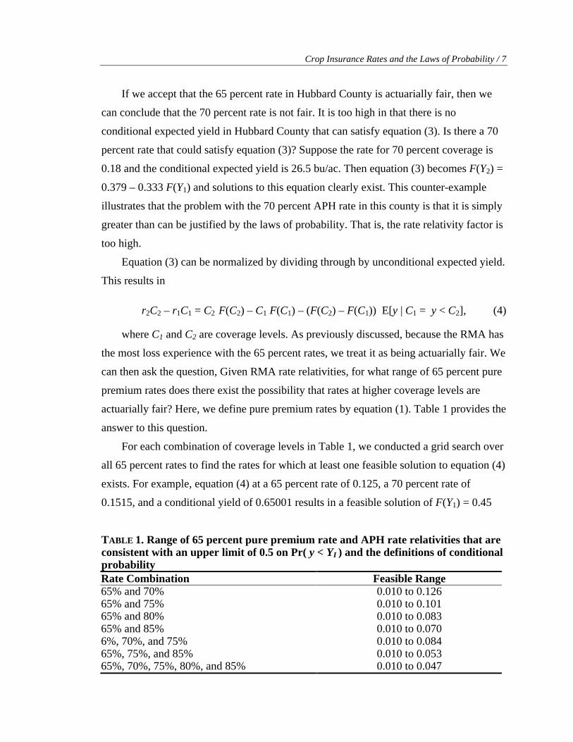
actuarially fair? Here, we define pure premium rates by equation (1). Table 1 provides the

answer to this question.

For each combination of coverage levels in Table 1, we conducted a grid search over

all 65 percent rates to find the rates for which at least one feasible solution to equation (4)

exists. For example, equation (4) at a 65 percent rate of 0.125, a 70 percent rate of

0.1515, and a conditional yield of 0.65001 results in a feasible solution of F(Y1) = 0.45

TABLE 1. Range of 65 percent pure premium rate and APH rate relativities that are consistent with an upper limit of 0.5 on Pr( y < YI ) and the definitions of conditional probability Rate Combination Feasible Range 65% and 70% 0.010 to 0.126 65% and 75% 0.010 to 0.101 65% and 80% 0.010 to 0.083 65% and 85% 0.010 to 0.070 6%, 70%, and 75% 0.010 to 0.084 65%, 75%, and 85% 0.010 to 0.053 65%, 70%, 75%, 80%, and 85% 0.010 to 0.047


and F(Y2) = 0.497. Of course, this solution means that there is almost no possibility of

having yields between 0.85 and 1.0, which illustrates the weakness of the conditions we

are imposing for actuarial fairness of rates.

The first four results in Table 1 show that as the coverage level increases, the range

of feasible 65 percent rates is reduced. This reduced range implies that the rate relativity

factors are becoming more restrictive as the coverage level increases. The 85 percent pure

premium rates can only be actuarially fair if the 65 percent rate is less than 0.07.

The pairwise consideration of rates in the first four rows of Table 1 puts no

restrictions on the underlying distribution function for intermediate coverage levels. If we

require that there be the possibility of actuarial fairness for intermediate coverage levels

as well, then the range of feasible 65 percent rates becomes even narrower. For example,

in counties where the maximum coverage level is 75 percent, the range of feasible 65

percent rates for which there is the possibility of actuarial fairness for the 65 percent rate,

the 70 percent rate, and the 75 percent rate is 0.01 to 0.084. If we require the possibility

of actuarial fairness for 65 percent, 75 percent, and 85 percent rates, then the maximum

65 percent rate is 0.053. And, if we require the possibility of actuarial fairness for all

coverage levels, then the maximum 65 percent rate is 0.047.

Effects of Further Restrictions

The maximum 65 percent rates reported in Table 1 were obtained by setting the

conditional yield equal to the minimum possible. This is equivalent to assuming that the

probability of yields between the considered coverage levels is zero. In addition, no

restrictions were placed on yields between 0.85 and 1.00. At the upper end of the ranges

reported in Table 1, there is no probability that yields would fall between 0.85 and 1.00.

This is illustrated in Figure 2, which shows graphs of the cumulative distribution function

(CDF) for yields given 65 percent insurance rates and conditional yields when yields falls

below 65 percent (denoted by CY 0 – 65). The yield distributions at the 65 percent rate of

0.047, which is at the upper end of the potentially acceptable range of rates for coverage

up to 85 percent, show little possibility of yields falling between 0.80 and 1.00, regardless

of the conditional yield level. The yield distribution at a 65 percent rate of 0.025, which is

in the middle of the Table 1 range, shows a more realistic distribution, with positive


weight across all coverage levels. For most distribution functions, one would expect the

bulk of probability to fall around the level of mean yields, although this is not necessarily

the case for bimodal distributions.

Given that the implied CDFs at the upper end of the ranges reported in Table 1 may

not conform to prior expectations about how yield distributions should look, we examine

five further restrictions regarding the probability of yields between the highest allowed

coverage level (0.75 or 0.85) and 1.00. These five scenarios are that the probability of

yields between the highest allowed coverage level and 1.00 is at least 0.05, 0.10, 0.15,

0.20, and 0.25. These scenarios provide a range of cases where some weight is distributed

just below the APH yield in the yield distributions. For example, a normal distribution

with a mean of 1.00 and a standard deviation of 0.25 would have 22.57 percent of its

weight between 0.85 and 1.00.

We also examine the effects of forcing convexity on the CDF of yields between 65

percent and 85 percent coverage. Convexity implies that the difference in cumulative

probabilities between two coverage levels increases as coverage increases: F(0.85) -

F(0.80) > F(0.80) - F(0.75) > F(0.75) - F(0.70) > F(0.70) - F(0.65). In addition to this

convexity restriction, we also assume that 0.5 - F(0.85) > F(0.85) - F(0.80). To impose

these conditions, we need to relate observed crop insurance rates to these cumulative

probabilities.

Rewriting equation (4) for C2 > C1 gives an expression for cumulative probability at

one coverage level as a function of cumulative probability at a lower coverage level and

the conditional expectation of yield given that yield is between the two coverage levels:

( ) (E[ | ] )( ) .

E[ | ]r C rC F C y C y C C

F CC y C y C

− − ≤ < −=

− ≤ <2 2 1 1 1 1 2 1

22 1 2

(5)

Given a conditional yield for yields below the 65 percent coverage level, we can

solve for F(0.65) using

0.65 0.65(0.65) .

0.65 [ | 0.65]r

FE y y

=− <

(6)

Then, F(0.70) as a function of the conditional yield between 65 percent coverage and

70 percent coverage can be obtained through direct substitution into equation (5).


Likewise, F(0.75), F(0.80), and F(0.85) can be obtained with subsequent substitutions.

All of the scenarios require a value for the conditional expectation of yield for yields

below the 65 percent coverage level and values for the conditional expectation of yields

between coverage levels. Convexity in cumulative probability implies that the expected

yield conditional on yield being between two coverage levels would typically be greater

than the midpoint of the coverage levels.

The task is to determine the range of feasible 65 percent rates that are consistent with

a given set of probability restrictions. This task can be accomplished by searching over

all possible values for expected yield conditional on yield being below 65 percent for

each given 65 percent rate. If any of the conditional yields are consistent with the

restrictions, then we can maintain that there is an underlying yield distribution that could

be consistent with APH rates.

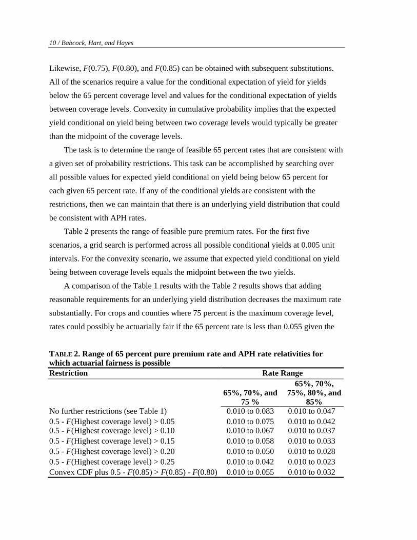
Table 2 presents the range of feasible pure premium rates. For the first five

scenarios, a grid search is performed across all possible conditional yields at 0.005 unit

intervals. For the convexity scenario, we assume that expected yield conditional on yield

being between coverage levels equals the midpoint between the two yields.

A comparison of the Table 1 results with the Table 2 results shows that adding

reasonable requirements for an underlying yield distribution decreases the maximum rate

substantially. For crops and counties where 75 percent is the maximum coverage level,

rates could possibly be actuarially fair if the 65 percent rate is less than 0.055 given the

TABLE 2. Range of 65 percent pure premium rate and APH rate relativities for which actuarial fairness is possible Restriction Rate Range

65%, 70%, and 75 %

65%, 70%, 75%, 80%, and

85% No further restrictions (see Table 1) 0.010 to 0.083 0.010 to 0.047 0.5 - F(Highest coverage level) > 0.05 0.010 to 0.075 0.010 to 0.042 0.5 - F(Highest coverage level) > 0.10 0.010 to 0.067 0.010 to 0.037 0.5 - F(Highest coverage level) > 0.15 0.010 to 0.058 0.010 to 0.033 0.5 - F(Highest coverage level) > 0.20 0.010 to 0.050 0.010 to 0.028 0.5 - F(Highest coverage level) > 0.25 0.010 to 0.042 0.010 to 0.023 Convex CDF plus 0.5 - F(0.85) > F(0.85) - F(0.80) 0.010 to 0.055 0.010 to 0.032


convexity restrictions. For crops and counties that have 85 percent coverage, the

maximum 65 percent rate for which actuarial fairness is possible is only 0.032 when the

convexity restrictions are put in place.

Which Crops and Counties Have Actuarially Unfair Rates?

Given the bounds on rates indicated in the previous section, we would like to

compare these bounds to current crop insurance rates throughout the country. However,

these bounds are based purely on yield distribution arguments and do not include

adjustments for insurance loading and prevented planting, whereas the current crop

insurance rates do contain such adjustments. To create comparable rates, we have

adjusted our bounds to reflect the insurance loading and prevented planting adjustments

by dividing by 0.88 to capture the insurance loading adjustment and adding 0.005 to the

rates to capture the prevented planting adjustment. These adjustments follow the rate-

setting procedure outlined in Josephson, Lord, and Mitchell.

For the “no further restriction” case, the adjusted insurance rates have maximum

bounds of 0.099 for areas with up to 75 percent coverage and 0.058 for areas with up to

85 percent coverage. For the restriction of at least a 15 percent probability of yields

falling between the highest coverage level and 1.0, the adjusted insurance rates have

maximum bounds of 0.071 for the areas with up to 75 percent coverage and 0.043 for the

areas with up to 85 percent coverage. We examined the crop year 2000 APH 65 percent

coverage level insurance rates for corn, soybeans, and wheat for the typical producer in

each county (as determined by the R05 yield span, the middle yield span per county for

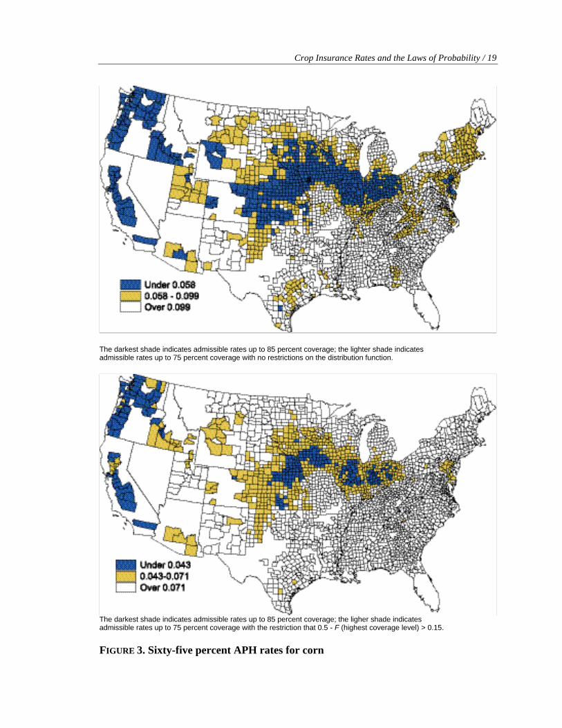
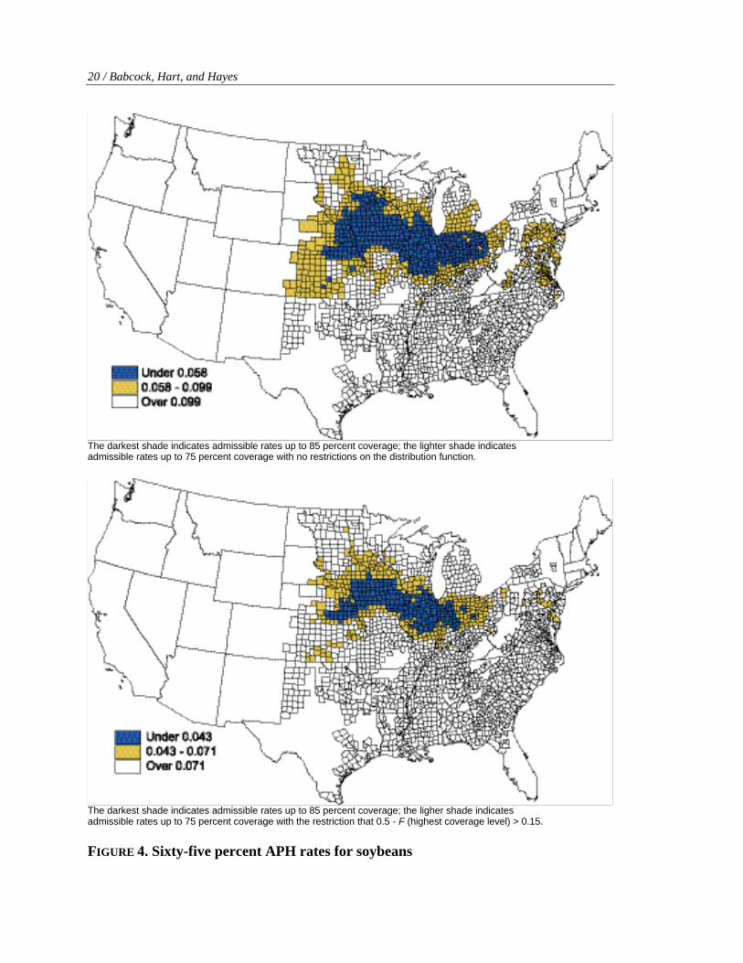
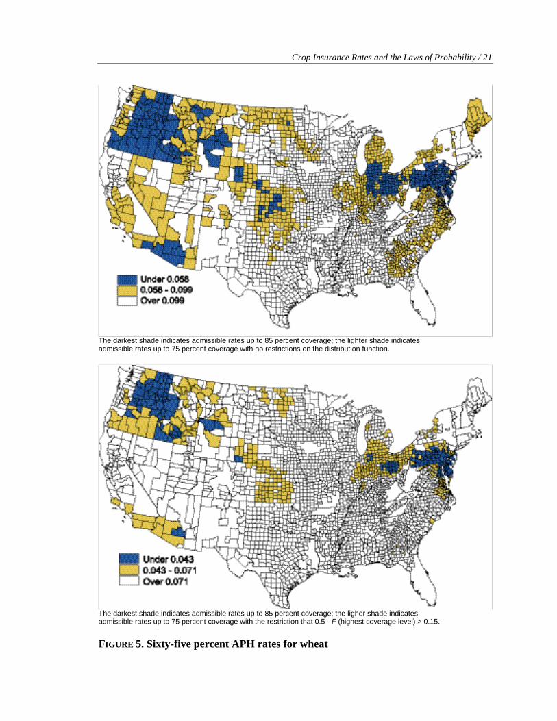
these crops). Figures 3-5 show maps of these rates across the country and whether they

fall into the bounds previously outlined. The counties shaded in dark blue have 65

percent APH rates that fall within the bounds set by a yield distribution with the 15

percent restriction in place for coverage levels from 65 percent to 85 percent. The

counties shaded in gold have 65 percent APH rates that fall within the bounds set by a

yield distribution with the 15 percent restriction in place for coverage levels from 65

percent to 75 percent. The counties shaded in white have 65 percent APH rates that

exceed either of these bounds. Counties that are not outlined do not have insurance

coverage for that crop. RMA provides these rates through their Actuarial Data Master


web site (http://www.rma.usda.gov/tools/utils/grepadm/). These 2000 rates are indicative

of current rates that are calculated with a formula without reference to a yield span.

Table 3 shows that most of the counties where APH insurance is available do not

have actuarially fair rates over all coverage levels. For corn, only 21.4 percent of the

counties have potentially fair rates up to 85 percent coverage, and 48.5 percent have

potentially fair rates up to 75 percent coverage. With the 15 percent probability

restriction, the proportions fall to 8.2 percent and 28.7 percent. As shown in Figure 3,

these counties primarily reside in the Corn Belt. The proportion of soybean and wheat

counties with potentially fair rates is similar, as shown in Table 3.

For corn and soybeans (see Figures 3 and 4), because the counties that have APH rates

that could be actuarially fair are located in the Corn Belt, the proportion of production that

they represent is high. For corn, almost 90 percent of production comes from counties that

could have actuarially fair rates up to 75 percent coverage, and almost 65 percent of

production comes from counties with APH rates that could be actuarially fair up to 85

TABLE 3. Proportion of counties and production with possibly actuarially fair APH premiums Criteriona Under 0.043 Under 0.058 Under 0.071 Under 0.099 Corn Number 207 540 725 1225 % of Counties 8.2 21.4 28.7 48.5 % of Production 29.1 64.8 77.5 89.7 Soybeans Number 190 351 473 808 % of Counties 9.7 17.8 24.0 41.0 % of Production 35.7 56.9 66.4 80.1 Wheat Number 121 291 500 1105 % of Counties 5.0 11.2 20.5 45.4 % of Production 11.2 23.0 41.9 70.2 a The level 0.043 corresponds to the upper limit on the APH rate for which actuarial fairness is possible for coverage levels up to 85% if at least 15% of probability is between 85% and 100% coverage levels. 0.058 is the upper limit on actuarially fair APH rates up to 85% coverage levels with no such probability restriction. 0.071 is the upper limit on actuarially fair APH rates up to 75% if at least 15% of probability is between 75% and 100% coverage levels. 0.099 is the upper limit on actuarially fair APH rates up to 75% coverage levels with no such probability restriction.


percent coverage. However, this latter number falls to 29 percent of production if the

reasonable 15 percent restriction is placed on the yield CDF. For soybeans, 36 percent of

production comes from counties with APH rates that could be fair up to 85 percent

coverage even with the 15 percent restriction. This estimate increases to 80 percent of

production for coverage to 75 percent and no other CDF restriction.

For wheat, the story is different. As shown in Figure 5, most of the major wheat

growing areas in Kansas and North Dakota have 65 percent APH rates that fall outside

the possible fair range for coverage levels up to 85 percent. Even without the 15 percent

probability restriction, only 23 percent of production comes from the 12 percent of the

counties with low enough 65 percent APH rates to be actuarially fair. Even at 75 percent

coverage with the 15 percent restriction, only 20 percent of the counties and 42 percent of

production have 65 percent APH rates that are low enough to be fair.

Based on the results of Table 3, one would expect that wheat farmers would have

been less likely than corn and soybean farmers to buy 75 percent coverage before the

additional ARPA subsidies were available for the simple reason that moving to 75

percent coverage meant that incremental costs exceeded incremental benefits.

Examination of RMA data bears out this conjecture. In 1998, 5.7 percent of wheat crop

insurance policies were at the 75 percent coverage level, as compared to 9.8 percent of

corn policies and 10.7 percent of soybean policies.

Rate Relativities Derived from a Density Function

A comparison of APH rate relativities with those derived from a density function

will illustrate why constant APH rate relativities are not consistent with the laws of

probability. The starting point is to select a density function.

Characterizing the distribution of farm-level yields has been the focus of much effort

by agricultural economists. Day demonstrated that crop yields are skewed, although Just

and Weninger demonstrated how data used to measure skewed yields is subject to a

number of possible problems. Day found that the beta distribution is an appropriate

functional form for parametric estimation purposes. Applied studies that have found the

beta distribution useful include Babcock and Blackmer, Borges and Thurman, Babcock

and Hennessy, and Coble et al.


The beta density function that describes the distribution of yield y, can be written

.yyyy

yyyyqp

qpyg qp

qp

maxmin1max

1max

1min where

)()()()(

)()( ≤≤

−−+= −+

−−

ΓΓΓ

where p, q, ymax, and ymin are the four parameters. Advantages of the beta distribution are

that it can exhibit both negative and positive skewness; it has finite minimum and

maximum values; and it can take on a wide variety of shapes, including J-shaped, and

normal-like.

What we want to accomplish is specification of beta parameters that are consistent

with a given pure premium rate at the 65 percent coverage level. We do this by first

relating the shape parameters, p and q, to the mean and standard deviation of farm yields,

and to the maximum and minimum yields. For a given ymax and ymin, p and q can be

obtained from mean yield µ (which was set to 1) and the standard deviation of yields, s ,

by the following two equations (Johnson and Kotz, p. 44):

minmax

min

1

2minmax

2

minmax

min

2

minmax

min

)(1

yyy

yyyyy

yyy

p−

−−

−

−

−−

−

−=

−µσµµ

.1)(

1 2minmax

2

minmax

min

minmax

min pyyyy

yyy

yq −−

−

−

−−

−−

=σµµ

We normalized mean yield to 1 and searched for the standard deviation of yields that

resulted in the 65 percent APH rate using Monte Carlo integration. Of course, the

maximum and minimum yields must be defined to identify a one-to-one mapping of yield

standard deviation to APH rate. This was accomplished with the following specifications:

ymin = max(1 – 4s , 0) and ymax = 1 + 2s . Thus, the search for a standard deviation that

generates the 65 percent APH rates is accomplished by imposing these two conditions on

the minimum and maximum yields.

The next step is to generate the appropriate yield distribution for a range of possible

APH rates. We chose a series of possible 65 percent APH rates ranging from 0.02 to 0.3.

An APH rate of 0.02 represents an extremely low risk production situation such as might

exist with irrigated corn. An APH rate of 0.3 represents the high-risk extreme.


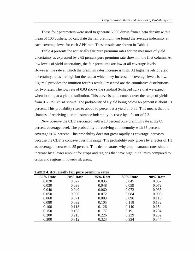
These four parameters were used to generate 5,000 draws from a beta density with a

mean of 100 bushels. To calculate the fair premium, we found the average indemnity at

each coverage level for each APH rate. These results are shown in Table 4.

Table 4 presents the actuarially fair pure premium rates for ten measures of yield

uncertainty as expressed by a 65 percent pure premium rate shown in the first column. At

low levels of yield uncertainty, the fair premiums are low at all coverage levels.

However, the rate at which the premium rates increase is high. At higher levels of yield

uncertainty, rates are high but the rate at which they increase in coverage levels is low.

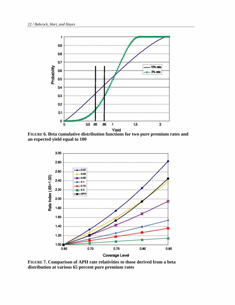
Figure 6 provides the intuition for this result. Presented are the cumulative distributions

for two rates. The low rate of 0.03 shows the standard S-shaped curve that we expect

when looking at a yield distribution. This curve is quite convex over the range of yields

from 0.65 to 0.85 as shown. The probability of a yield being below 65 percent is about 13

percent. This probability rises to about 30 percent at a yield of 0.85. This means that the

chances of receiving a crop insurance indemnity increase by a factor of 2.3.

Now observe the CDF associated with a 10 percent pure premium rate at the 65

percent coverage level. The probability of receiving an indemnity with 65 percent

coverage is 32 percent. This probability does not grow rapidly as coverage increases

because the CDF is concave over this range. The probability only grows by a factor of 1.3

as coverage increases to 85 percent. This demonstrates why crop insurance rates should

increase by a lesser amount for crops and regions that have high initial rates compared to

crops and regions in lower-risk areas.

TABLE 4. Actuarially fair pure premium rates 65% Rate 70% Rate 75% Rate 80% Rate 90% Rate

0.020 0.027 0.035 0.045 0.057 0.030 0.038 0.048 0.059 0.072 0.040 0.049 0.060 0.072 0.085 0.050 0.060 0.072 0.084 0.098 0.060 0.071 0.083 0.096 0.110 0.080 0.092 0.105 0.118 0.132 0.100 0.113 0.126 0.140 0.154 0.150 0.163 0.177 0.191 0.204 0.200 0.213 0.226 0.239 0.252 0.300 0.312 0.323 0.334 0.344


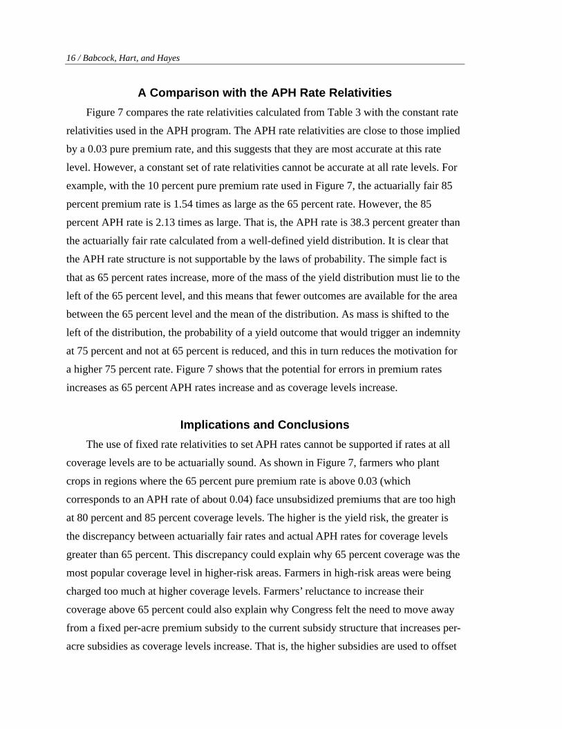
A Comparison with the APH Rate Relativities

Figure 7 compares the rate relativities calculated from Table 3 with the constant rate

relativities used in the APH program. The APH rate relativities are close to those implied

by a 0.03 pure premium rate, and this suggests that they are most accurate at this rate

level. However, a constant set of rate relativities cannot be accurate at all rate levels. For

example, with the 10 percent pure premium rate used in Figure 7, the actuarially fair 85

percent premium rate is 1.54 times as large as the 65 percent rate. However, the 85

percent APH rate is 2.13 times as large. That is, the APH rate is 38.3 percent greater than

the actuarially fair rate calculated from a well-defined yield distribution. It is clear that

the APH rate structure is not supportable by the laws of probability. The simple fact is

that as 65 percent rates increase, more of the mass of the yield distribution must lie to the

left of the 65 percent level, and this means that fewer outcomes are available for the area

between the 65 percent level and the mean of the distribution. As mass is shifted to the

left of the distribution, the probability of a yield outcome that would trigger an indemnity

at 75 percent and not at 65 percent is reduced, and this in turn reduces the motivation for

a higher 75 percent rate. Figure 7 shows that the potential for errors in premium rates

increases as 65 percent APH rates increase and as coverage levels increase.

Implications and Conclusions

The use of fixed rate relativities to set APH rates cannot be supported if rates at all

coverage levels are to be actuarially sound. As shown in Figure 7, farmers who plant

crops in regions where the 65 percent pure premium rate is above 0.03 (which

corresponds to an APH rate of about 0.04) face unsubsidized premiums that are too high

at 80 percent and 85 percent coverage levels. The higher is the yield risk, the greater is

the discrepancy between actuarially fair rates and actual APH rates for coverage levels

greater than 65 percent. This discrepancy could explain why 65 percent coverage was the

most popular coverage level in higher-risk areas. Farmers in high-risk areas were being

charged too much at higher coverage levels. Farmers’ reluctance to increase their

coverage above 65 percent could also explain why Congress felt the need to move away

from a fixed per-acre premium subsidy to the current subsidy structure that increases per-

acre subsidies as coverage levels increase. That is, the higher subsidies are used to offset


the excessive premium charge, making higher coverage levels more attractive. If APH

rates were made actuarially fair by allowing rate relativities to vary by crop and region,

then perhaps Congress could revert to fixed per-acre subsidies, which would induce

farmers to select the crop insurance product that gives them the biggest risk management

return per premium dollar rather than having that decision distorted by proportionate

premium subsidies.

The increased subsidies under ARPA have brought increased public attention to the

implications of an unsound APH rate structure. For example, Barnaby demonstrated that

Revenue Assurance (RA) with the harvest price option could actually cost 20 percent less

than simple yield insurance and 32 percent less than CRC for Kansas dryland corn

production at 85 percent coverage. Farmers in these regions must settle for lower

coverage, or they may find that increased subsidies available at higher coverage levels

offset the excessive unsubsidized premium.


FIGURE 1. Net acres insured under the APH program

FIGURE 2. Graphs of cumulative distribution functions at various insurance rates and conditional yields


The darkest shade indicates admissible rates up to 85 percent coverage; the lighter shade indicates admissible rates up to 75 percent coverage with no restrictions on the distribution function.

The darkest shade indicates admissible rates up to 85 percent coverage; the ligher shade indicates admissible rates up to 75 percent coverage with the restriction that 0.5 - F (highest coverage level) > 0.15. FIGURE 3. Sixty-five percent APH rates for corn



The darkest shade indicates admissible rates up to 85 percent coverage; the ligher shade indicates admissible rates up to 75 percent coverage with the restriction that 0.5 - F (highest coverage level) > 0.15. FIGURE 4. Sixty-five percent APH rates for soybeans



The darkest shade indicates admissible rates up to 85 percent coverage; the ligher shade indicates admissible rates up to 75 percent coverage with the restriction that 0.5 - F (highest coverage level) > 0.15. FIGURE 5. Sixty-five percent APH rates for wheat


FIGURE 6. Beta cumulative distribution functions for two pure premium rates and an expected yield equal to 100

FIGURE 7. Comparison of APH rate relativities to those derived from a beta distribution at various 65 percent pure premium rates

References

Babcock, B. A., and A. M. Blackmer. “The Value of Reducing Temporal Input Nonuniformities.” Journal of Agricultural and Resource Economics 17(December 1992): 335-47.

Babcock, B. A., and D. Hennessy. “Input Demand Under Yield and Revenue Insurance.” American Journal of Agricultural Economics 78(May 1996): 416-27.

Barnaby, A. Presentation made at the Commodity Classic, Nashville, TN, Feb. 25, 2002. http://www.agecon.ksu.edu/risk/ (accessed March 2002).

Borges, R. B., and W. N. Thurman. “Marketing Quotas and Subsidies in Peanuts.” American Journal of Agricultural Economics 76(November 1994): 809-17

Coble, K. H., T. O. Knight, R. D. Pope, and J. R. Williams. “Modeling Farm-Level Crop Insurance Demand with Panel Data.” American Journal of Agricultural Economics 78(May 1996): 439-47.

Day, R. H. “Probability Distributions of Field Crops.” Journal of Farm Economics 47(1965): 713-41.

Johnson, N. L., and S. Kotz. Continuous Univariate Distributions-2. New York: John Wiley and Sons, 1970.

Josephson, G. R., R. B. Lord, and C. W. Mitchell. “Actuarial Documentation of Multiple Peril Crop Insurance Ratemaking Procedures.” Report prepared for the U.S. Department of Agriculture, Risk Management Agency, by Milliman and Robertson, Inc, 2001. http://www.rma.usda.gov/pubs/2000/MPCI_Ratemaking.pdf (accessed March 2002).

Just, R. E., L. Calvin, and J. Quiggin. “Adverse Selection in Crop Insurance.” American Journal of Agricultural Economics 81(November 1999): 835-49.

Just, R.E., and Q. Weninger. “Are Crop Yields Normally Distributed?” American Journal of Agricultural Economics 81(May 1999): 287-304.

Crop Insurance Rates and the Laws of Probability

Documents

Transcript of Crop Insurance Rates and the Laws of Probability