RUSSIAN JOURNAL OF EARTH SCIENCES, VOL. 19, ES6007, doi:10.2205/2019ES000651, 2019

Kaula’s rule – a consequence of probability laws byA. N. Kolmogorov and his school

E. B. Gledzer1 and G. S. Golitsyn1

Received 18 January 2019; accepted 28 November 2019; published 12 December 2019.

The paper analyzes a possible cause for the universal behavior of the covariatingfluctuations of planet gravity. The consideration based on the idea that the topographyfluctuations are governed by a random Markov process leads to universal dependence𝑘−2with 𝑘 being the amplitudes of the 𝑗-th spherical harmonic of the terrain profile.This law known as the Kaula’s rule is then derived from the solution of the Fokker –Plank equation for the fluctuations of the terrain profile as the function of the horizontalcoordinate. The respective diffusivities for Earth and Venus are retrieved from theexisting data. KEYWORDS: Kaula’s rule; Thumb rule; planet gravity; Fokker-Planck

equation.

Citation: Gledzer, E. B. and G. S. Golitsyn (2019), Kaula’s rule – a consequence of probability laws by

A. N. Kolmogorov and his school, Russ. J. Earth. Sci., 19, ES6007, doi:10.2205/2019ES000651.

Introduction

The Kaula’s rule [Kaula, 1966] sometimes called“the rule of thumb” exists for over half a century.However, its origin is unknown. In its original formit claims that the terrestrial gravity field fluctu-ations expanded in spherical harmonics have thespectral asymptotics proportional to 𝑗−2, where 𝑗is the number of the harmonic. Similar behaviorwas established to hold on Moon, Mars [Rexer andHirt, 2015], and Venus [Turcotte, 1997]. In thisdecade the same property has been found for as-teroid Vesta whose diameter does not exceed 300km [Konopliv et al., 2014] and for asteroids of fewkilometers in size [McMahon et al., 2016]. In later1980-s it was found that surface reliefs of Earth andVenus have the same 𝑗−2 asymptotics [Turcotte,1997]. In [Rexer and Hirt, 2015] the harmonicswith 𝑗 up to tens thousands have been computed.This means that gravity field fluctuations and re-lief are connected. Therefore “the rule of thumb”

1A. M. Obukhov Institute of Atmospheric PhysicsRAS, Moscow, Russia.

Copyright 2019 by the Geophysical Center RAS.

http://rjes.wdcb.ru/doi/2019ES000651-res.html

is expected to be a law whose nature still awaitingfor explanation.Here we use the Fokker – Planck equation in the

form presented by A. N. Kolmogorov, [1934] andits further results of its statistical analysis devel-oped by his pupils A. M. Obukhov [Obukhov, 1959]and by A. S. Monin and A. M. Yaglom, 1975]. Thebasic equation formulated in [Kolmogorov, 1934] ismore general than it is necessary here. Later thisequation was used for studying other natural phe-nomena: like turbulence in [Obukhov, 1959], andrecently sea wind waves spectra, the cumulativedistribution of litospheric plates, etc. in [Golit-syn, 2018]. This impelled us to return to an at-tempt to derive analytically the Kaula’s rule. Forreader’s convenience we present the description ofideas and methods of [Kolmogorov, 1934; Obukhov,1959; Monin and Yaglom, 1975] rarely used in gen-eral geophysics but still appearing in various papersand books during past decades.

Basic Equations

In the beginning of 1930-s A. N. Kolmogorov hadpublished three papers on analytical methods in

ES6007 1 of 8

ES6007 gledzer and golitsyn: kaula’s rule ES6007

the probability theory. The two-page work [Kol-mogorov, 1934] contains the essence of his approachstarted by A. Einstein and developed further byFokker and Planck. Kolmogorov proposed a fun-damental solution to the evolution equation for theprobability distribution 𝑝(𝑢𝑖, 𝑥𝑖, 𝑡) of the 6D vector𝑢, 𝑥 provided a delta correlated force causes the re-spective Markov process. This is an approximationof the processes where correlation time of the ran-dom forces is much shorter than the reaction timeof the considered system. In 1D approximation theaction of respective random accelerations 𝑎𝑡 with⟨𝑎(𝑡1)𝑎(𝑡2)⟩ = 𝑎2𝛿(𝑡1 − 𝑡2) can be described by thesimplest equations [Gledzer and Golitsyn, 2010],

𝑑𝑢(𝑡)

𝑑𝑡= 𝑎(𝑡),

𝑑𝑥(𝑡)

𝑑𝑡= 𝑢(𝑡), (1)

where 𝑢(𝑡) and 𝑥(𝑡) are the velocity and displace-ment of a particle under random acceleration 𝑎(𝑡).A. N. Kolmogorov used a Fokker-Planck type

equation [Kolmogorov, 1934] to describe the evo-lution of the probability density 𝑝(𝑢𝑖, 𝑥𝑖, 𝑡),

𝜕𝑝

𝜕𝑡+ 𝑢𝑖

𝜕𝑝

𝜕𝑥𝑖= 𝐷

𝜕2𝑝

𝜕𝑢2𝑖, (2)

where 𝐷 is a coefficient of diffusion in the veloc-ity space. The fundamental solution2 to eq. (2)has the form (see also [Monin and Yaglom, 1975],S24.4):

𝑝(𝑢𝑖, 𝑥𝑖, 𝑡) =

( √3

2𝜋𝐷𝑡2

)3

× (3)

× exp

[−(𝑢2𝑖𝐷𝑡

− 3𝑢𝑖𝑥𝑖𝐷𝑡2

+3𝑥2𝑖𝐷𝑡3

)].

A. M. Obukhov [Obukhov, 1959] was the firstwho analyzed and used this equation. He showedthat the coefficient 𝐷 is proportional to the gen-eration/dissipation rate of the kinetic energy ofthe random motions 𝐷 = 𝜀/2. The details ofhis analysis are presented in [Monin and Yaglom,1975; Golitsyn, 2018]. The solution (3) demon-strates that the seeked probability distribution hasthe normal character. This solution has two scales(angular brackets mean ensemble averaging):⟨

𝑢2𝑖⟩= 𝜀𝑡,

⟨𝑥2⟩≡ 𝑟 = 𝜀𝑡3, 𝜀 = 2𝐷. (4)

2 In the original paper [Kolmogorov, 1934] the mid-dle term under exponent was absent.

Figure 1. Temporal behaviour of the second ve-locity and coordinate moments for different par-ticle ensemble sizes as in [Gledzer and Golitsyn,2010] (see text).

Combining the scales for velocity and coordi-nates Obukhov formulated the scale for the mixedmoment ⟨𝑢𝑖𝑥𝑖⟩ = 𝐾 in terms of 𝜀 as

𝐾 = 𝜀𝑡2. (4’)The time dependencies eqs (4) and (4’) were ver-

ified numerically for the ensembles of 𝑁 randomlymoving particles [Gledzer and Golitsyn, 2010]. Fig-ure 1 demonstrates that even for 𝑁 = 10 the rela-tionships (4) fulfil satisfactorily as it is shown inFigure 1. Moreover, on introducing the dimen-sionless variables to non-dimensional ones (denotedwith tilde overhead)

𝑡 = 𝑡𝜏, 𝑢 = ��(𝜀𝜏)1/2, 𝑟 = 𝑟(𝜀𝜏3)1/2

reduces eq. (2) to the universal or selfsimilar form[Gledzer and Golitsyn, 2010]

𝜕𝑝

𝜕𝑡+ ��

𝜕𝑝

𝜕𝑟=

1

2

𝜕2𝑝

𝜕��2. (5)

The scales (4) can be interpreted as the struc-ture functions with zero initial conditions whichallow us to introduce their spectral forms [Moninand Yaglom, 1975]. If we replace 𝑡 by 𝑟 (see eq.(4)), exclude time from the second scale (4) andput it into the first scales and to (4’) and substi-tute the result into eq. (4’), we obtain the resultsof Kolmogorov – Obukhov of 1941 𝐷𝑢(𝑟) = (𝜀𝑟)2/3

and Richardson – Obukhov [Obukhov, 1941; 1959;

2 of 8

ES6007 gledzer and golitsyn: kaula’s rule ES6007

Richardson, 1926; 1929] for the eddy diffusion co-efficient:

𝐾(𝑟) = 𝜀1/3𝑟4/3. (6)

These are the results for the inertial interval ofturbulence. The results as relations (4) are valid ir-respective of the space dimension and the numericsprove it [Gledzer and Golitsyn, 2010]. It is surpris-ing that since 1920s nobody tried to understandwhy the Richardson’s “law of – 4/3” holds up to 2–3thousands km in the horizontal direction [Richard-son, 1926; 1929], i. e. the vertical component andfull velocity isotropy are not important. In 1999Lindborg [Lindborg, 2008] analyzed the experimen-tal data of commercial flights in terms of struc-ture functions. He showed that the dependence𝑟2/3 is traced up to distances of 2 thousands km.His results in terms of the eddy diffusion explainthe Richardson results of 1920-s. These facts canbe explained starting with a two-page note of Kol-mogorov, 1934 [Kolmogorov, 1934], and the follow-ing development of his results by Obukhov, [1959]and Monin and Yaglom, [1975]. Only the Markovproperties of the process are important rather thanthe full isotropy except in horizontal direction. Ournumerics of 2010 [Gledzer and Golitsyn, 2010] con-firmed this independence of the space dimension-ality for the second moments with the accuracy ofthe numerical coefficients up to 0 (1).

Spectral Representations

For further development we need an analyticalconnection between the second moments and theirspectral representations when both of them arepower laws. Let us consider first the structure func-tion 𝐷(𝑡) = 𝐴𝑡𝛾 , 0 < 𝛾 < 2. The relation to thespectrum is [Monin and Yaglom, 1975]

𝐷(𝑡) = 2

∫ ∞

0(1− cos𝜔𝑡)𝐸(𝜔)𝑑𝜔, (7)

The inversion gives for the spectrum [Monin andYaglom, 1975; Yaglom, 1955; 1986]:

𝐸(𝜔) =𝐶

𝜔𝛾+1, 𝐶 =

𝐴

𝜋Γ(𝛾 + 1) sin

𝜋𝛾

2, (8)

where Γ is the gamma function. The length scalerelated to the mean square displacement of a ran-domly moving particle has therefore the spectrum

𝐶𝜔−4, 𝐶 = 𝐴/𝜋 and for the velocity scale⟨𝑢2⟩= 𝜀𝑡

the spectrum is 𝜀𝜔−2. According to the terminol-ogy introduced by Yaglom, [1955; 1986] the spec-trum 𝜔−2 corresponds to a process with stationaryincrements of the first order (0 < 𝛾 < 2), whilethe spectrums 𝜔−4 has the stationary incrementsof the second order (2 < 𝛾 < 4). In order to avoidthe singularity at 𝜔 → 0 the transformation kernelin eq. (7) should be (1 − 𝑐𝑜𝑠𝜔𝑡)𝑛, with 𝑛 = 1 forvelocities, and 𝑛 = 2 for coordinates.

Toward Thumb Rule

When a flying altimeter measures the relief, weobtain a temporal variations of height signal ℎ(𝑡).The time 𝑡 here is related to horizontal coordinateas 𝑦 = 𝑢𝑡, 𝑢 being the flight velocity. The standardFokker – Planck equation with stochastic velocityfluctuations in this case is

𝜕𝑝

𝜕𝑡= 𝐷

𝜕2𝑝

𝜕ℎ2

If 𝑦 = 𝑢𝑡 it transforms to

𝜕𝑝

𝜕𝑦= 𝐷1

𝜕2𝑝

𝜕ℎ2, 𝐷1 =

𝐷

𝑢. (9)

The diffusion coefficient 𝐷1 has the dimensionof length. But if the vertical 𝐿𝑧 and horizontal𝐿𝑦 scales are different, then 𝐷1 = 𝐿2

𝑧/𝐿𝑦 whichreflexes clearly the diffusion character of the reliefformation process during millions years. Equation(9) yields the scale and the structure functions forzero initial condition in the form:⟨

ℎ2(𝑦)⟩= 𝐷1𝑦

with the corresponding spectrum

𝑆(𝑘) = 𝐷1𝑘−2, 𝑘 = 2𝜋/𝜆𝑦, (10)

𝜆𝑦 being the corresponding horizontal wave length.This equations applicable for small scale contin-uous areas. The spectrum of the relief slopes inthis approximation is 𝑆𝜁(𝑘) = 𝑘2𝑆(𝑘) = 𝐷 =𝑐𝑜𝑛𝑠𝑡. The constancy of a spectrum is referred toas “white noise”. The slope of the relief

𝑑ℎ(𝑦)

𝑑𝑦= 𝜍(𝑦) (11)

3 of 8

ES6007 gledzer and golitsyn: kaula’s rule ES6007

for which we accept the hypothesis of 𝛿-correlatedhorizontal coordinates

⟨𝜍(𝑦1)𝜍(𝑦2)⟩ = 𝜍2𝛿(𝑦1 − 𝑦2) (12)

Equation (12) corresponds to the Markov charac-ter of forces in [Kaula, 1966; Rexer and Hirt, 2015;Turcotte, 1997]. Here 𝜍2 may be interpreted as themean square slope angle, a dimensionless value.Now we return to the reliefs of concrete planets.

Recently an extensive paper on ultrahigh sphericalharmonics analysis for topography of Earth, Marsand Moon has appeared [Rexer and Hirt, 2015]with the horizontal resolution up to hundreds ofmeters. Much earlier analyses of topography forEarth and Venus were given in [Turcotte, 1997]. Inthat book there are also the data for mountain,hilly and plain areas of hundred kilometers in sizeat the Oregon state. The flights were done in vari-ous directions in each type of terrain. For recordsin the range 1 – 60 km the mean exponent valueof these spectra were found [Golitsyn, 2003] to be2.03 ± 0.04. Unfortunately, there were no data in[Turcotte, 1997] for spectral amplitudes. Obviously𝑘−2 small size spectrum is a continuation of whatKaula found for large scale harmonics.In the book [Turcotte, 1997] the spectral ex-

ponent 2 (and other statistical measures, such asHausdorff measure, the fractal index 𝑑) were re-trieved from the original records. But no explana-tion of particular values was proposed.The analysis done by Kolmogorov [Kolmogorov,

1934; Monin and Yaglom, 1975] several decadesearlier was clearer and simpler. The only assump-tion on 𝛿-correlation of slopes applies for the pro-cesses in consideration, i.e. the Markov’s hypothe-sis. Such assumption is used in many branches oftheoretical physics meaning only that the systemreaction time is much larger than the correlationtime of stochastic influence on it [Golitsyn, 2003].

Spherical Harmonics

For large planetary scale features the sphericalharmonic analysis is used. Let us consider the reliefon a sphere 𝑧(𝜙, 𝜃) with a radius 𝑟, where 𝜙 islongitude, 0 ≤ 𝜙 < 2𝜋, 𝜃 is a co-latitude, 0 ≤ 𝜃 ≤𝜋. Then

𝜕𝑧(𝜙, 𝜃)

𝑟𝜕𝜃= 𝜍𝜃(𝜙, 𝜃)

is the slope angle. Let us introduce 𝑥 = cos 𝜃 andpresent the relief as a sum of normalized associated

Legendre polinomials 𝑃|𝑚|𝑗 (𝑥),

𝑧(𝜙, 𝜃)

𝑟= −

∞∑𝑗=1

𝑗∑𝑚=−𝑗

𝑎𝑗𝑚 exp(𝑖𝑚𝜙)Φ|𝑚|𝑗 (𝑥), (13)

Φ|𝑚|𝑗 (𝑥) = 𝑁

|𝑚|𝑗 𝑃

|𝑚|𝑗 (𝑥),

∫ 1

−1Φ|𝑚|𝑗 (𝑥)Φ

|𝑚|𝑖 (𝑥)𝑑𝑥 = 𝛿𝑗𝑖, 𝑁

|𝑚|𝑗 =(

2𝑗 + 1

2

(𝑗 − |𝑚|)!(𝑗 + |𝑚|)!

)1/2

.

Then due to eq. (13) the relief slope is expressedthrough the derivative,

𝜁𝜃(𝜑, 𝜃) =

∞∑𝑗=1

𝑗∑𝑚=−𝑗

𝑎𝑗𝑚 exp(𝑖𝑚𝜙) sin 𝜃𝑑Φ

|𝑚|𝑗 (𝑥)

𝑑𝑥.

(14)Consider the mean normalized energy (in quad-

ratic sense) of the relief slopes as follows,

𝐸𝜃 =

∫ 2𝜋

0

∫ 1

−1< 𝜁2𝜃 > 𝑑𝜙𝑑𝑥 = (15)

2𝜋

∞∑𝑗=1

𝑗∑𝑚=−𝑗

< |𝑎𝑗𝑚|2 >∫ 1

−1(1− 𝑥2)

(𝑑Φ

|𝑚|𝑗 (𝑥)

𝑑𝑥

)2

𝑑𝑥.

We consider the mean values of the spectral com-ponents< |𝑎𝑗𝑚|2 > to be independent of𝑚, which isconfirmed by observations and on practice [Kaula,1966; Rexer and Hirt, 2015; Turcotte, 1997]. It thusdepends only meridional index 𝑗 and can be foundon summing over longitudinal index 𝑚:

< |𝑎𝑗𝑚|2 >=𝛼2

𝑗(𝑗 + 1)(𝑗 + 1/2), (16)

where 𝛼 is the mean angle of the relief slope. Tak-ing this into account and calculating the integralsin eq. (15) we have on summing over 𝑚

𝐸𝜃 = 2𝜋

∞∑𝑗=1

𝑆𝑗 , 𝑆𝑗 =𝛼2

𝑗(𝑗 + 1), (17)

4 of 8

ES6007 gledzer and golitsyn: kaula’s rule ES6007

We thus obtain the constant spectrum of “white-noise”, i.e. 𝛿-correlation of 𝜃 Then for the reliefenergy (as mentioned above), we derive a quadraticvalue integrated over the spectrum from (13),

𝐸 =

∫ 2𝜋

0

∫ 1

−1< 𝑧2 > 𝑑𝜙𝑑𝑥 = (18)

2𝜋𝑟2∞∑𝑗−1

𝑗∑𝑚=−𝑗

< |𝛼𝑗𝑚|2 >

∫ 1

−1(Φ

|𝑚|𝑗 (𝑥))2𝑑𝑥 =

2𝜋𝑟2∞∑𝑗−1

𝑗∑𝑚=−𝑗

< |𝛼𝑗𝑚|2 > .

It is clear from here that the mean of the spec-tral components (17) provides the spectrum relief∼ 𝑗−2 at 𝑗 >> 1, as was found from the empiri-cal data of refs [Kaula, 1966; Konopliv et al., 2014;McMahon et al., 2016; Rexer and Hirt, 2015; Tur-cotte, 1997].

𝐸 = 2𝜋

∞∑𝑗=1

𝑗∑𝑚=−𝑗

𝑟2𝑎2

𝑗(𝑗 + 1)(𝑗 + 1/2)= (19)

2𝜋

∞∑𝑗=1

𝑟2𝑎2(2𝑗 + 1)

𝑗(𝑗 + 1)(𝑗 + 1/2)=

4𝜋

∞∑𝑗=1

𝑟2𝑎2

𝑗(𝑗 + 1)= 4𝜋𝑟2𝛼2 = 4𝜋𝑟𝐷1,

Here𝐷1 is the horizontal diffusion coefficient and∞∑𝑗=1

1

𝑗(𝑗 + 1)= 1 (note 1

𝑗(𝑗+1) =1

𝑗− 1

𝑗 + 1iden-

tity). The dependence of our harmonic coefficients1/𝑗(𝑗 + 1) (see eq. (19)) differs from Kaula’s 1/𝑗2

by the factor 1/𝑗2(𝑗 + 1). At 𝑗 = 4 it is equal to1/80.In order to replace integers 𝑗 by continuous wave

numbers 𝑗 at 𝑗 → ∞, i.e. for small horizontalscales, we shall use in eq. (13) the asymptotics of

the polynoms 𝑃|𝑚|𝑗 (cos 𝜃) at 𝑗 → ∞ :

𝑃|𝑚|𝑗 (cos 𝜃) ≈ (−1)𝑚

(2

𝜋𝑗 cos 𝜃

)1/2

× (20)

× cos(𝛼− 𝜋

4+

𝑚𝜋

2

), 𝛼 =

(𝑗 +

1

2

)𝜃

Now instead of co-latitude 𝜃 we will use thelength 𝑦 along the meridian assuming 𝜃 = 0 atthe north pole,

𝑦 = 𝑟𝜃, 0 ≤ 𝜃 < 𝜋. (21)

Then we rewrite the phase 𝛼 in eq. (20) as 𝛼 =𝑦𝑑𝑘(𝑗 + 1

2), where 𝑑𝑘 = 𝑗𝑟 is an increment of the

wave number 𝑘 = 𝑗 · 𝑑𝑘 at 𝑗 → ∞. Then for verysmall horizontal scales one has at 𝑑𝑘 → ∞,

𝛼 = 𝑘𝑦, 𝑘 = 𝑗 · 𝑑𝑘 = 𝑗/𝑟 (22)

Now let us apply the wave number 𝑘 in the eq.(18) for the relief energy. At 𝑗 → ∞ we obtain

𝐸 = 2𝜋𝐷1𝑘−2 = 4𝜋𝑟𝛼2𝑘−2. (23)

Here 4𝜋𝑟𝛼2𝑘−2 = 𝑆(𝑘) is the spectrum with di-mension of the cubic length (recall that 𝛼 the rmsslope angle). It can be seen that the value 𝑟𝛼2 ineq. (23) is proportional to the diffusion coefficient𝐷1 in the coordinate space.The relief spectrum in eq. (19) differs from the

Kaula’s “rule of the thumb” ∝ 𝑗−2 by the multi-plier [𝑗(𝑗 + 1)]−1. The relative difference betweenthe two at 𝑗 → ∞ decreases as [𝑗2(𝑗+1)]−1 but forsmall 𝑗 it is quite noticeable, e.g. at 𝑗 = 1 the dif-ference is 1/2, and at 𝑗 = 4 it is 20%. This showsthat the hypothesis on the “white noise” of therelief slope angles is not accurate at these scales.Thus the corresponding relief structure at 𝑗 ≤ 5could be different for each celestial body due to itspeculiar tectonics.

Results and Discussion

Our scheme of the relief evolution basing on eq.(9) of the probability density changes is the hor-izontal diffusion of the tectonically formed verti-cal structure under the gravity acting along slopes.Slopes as a measure of forces resist to winds; waterand rocks are running down along them, etc. Fig-ure 2 (Figure 7.19 from [Turcotte, 1997]) presentsthe amplitudes of the relief spherical harmonics:for Earth 𝑗 ≤ 180 and for Venus 𝑗 ≤ 50. At 𝑗 ≥ 4all coefficients approach to the inverse square de-pendence.We compare our theoretical expression for har-

monic coefficients from eq. (19)

5 of 8

ES6007 gledzer and golitsyn: kaula’s rule ES6007

Figure 2. Relief spectral harmonics for Earth andVenus after [Turcotte, 1997].

𝑆𝑗 =4𝜋𝑟𝐷1

𝑗(𝑗 + 1)(24)

to their empirical values from Figure 2.The comparison has been done for selected har-

monics with accuracy about 10% within their valueorder. The harmonic numbers for Earth were 5, 10,20, 30, 40, 60, 90. This produced 𝐷1 = 1.3 ± 0.3m. For Venus the numbers 5, 10, 15, 20, 30, 40and 50 produced 𝐷1 = 0.19 ± 0.03 m. Our diffu-sion coefficient is determined with accuracy about20%. The striking difference between these twoplanets has been already noted by [Turcotte, 1997].However, one should recall that Venusian data are

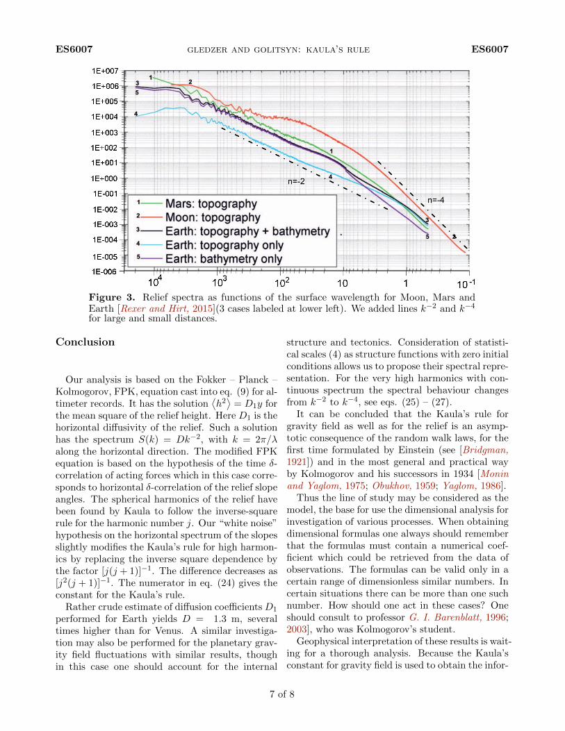
related only to equatorial plates [Turcotte, 1997].The global relief characteristics can be estimatedwith much higher precision and efforts (see e.g.[Rexer and Hirt, 2015]), which we leave for muchyounger colleagues, but we believe that it would beworth doing.Figure 3 presents the relief spectra as the func-

tions of the surface linear wave length 𝑘. Theauthors of [Rexer and Hirt, 2015] have computedspherical harmonics for Earth and Moon up to 𝑗 =46200 and for Mars up to 𝑗 = 23100. Our eqs. (20)– (23) present high frequency harmonics in termsof 𝑘−2. At Figure 3 we added straight lines cor-responding to the spectra 𝑘−2 and 𝑘−4, the lastfor very high wave numbers. The dependence 𝑘−2

holds well for Mars, line 1, and for three terrestrialspectra, lines 3-5, with some steeping for wavesshorter than a few kilometers. The Moon spectrumfalls down and remains almost flat at 200 – 80 km,being very specific in this respect. This evidencesthat the Moon is bombarded by the asteroids thesize of about 10 km, since the size of a crater is10-20 times exceeds the diameter of the asteroid.The explanation for the relief spectral decrease

from 𝑘−2 to 𝑘−4 can be explained by rejecting the𝛿-correlation for the relief slopes hypothesis. Thesimplest correlation function is

𝐵𝜃(𝜃(𝑦1)𝜃(𝑦2)) ∼ exp(−𝛽𝑦), 𝑦 = 𝑦2 − 𝑦1, (25)

where 𝛽 ≈ 1/ℎ and ℎ is mean relief height. Itsspectrum is

𝑆𝜃(𝑘) =𝛽

𝜋(𝛽2 + 𝑘2), (26)

and if we know the spectrum of the derivatives,i. e. angles, the spectrum of the value itself, relief,would be

𝑆𝜃(𝑘) = 𝑘2𝑆2𝜃 (𝑘) =

𝑘−2𝛽

𝜋(𝛽2 + 𝑘2). (27)

This spectrum has both right asymptotes: atℎ2 ≪ 𝛽2 it would be proportional to 𝑘−2 and ininverse case for small distances it ∼ 𝑘−4. The grav-ity acceleration on the Moon is six times weakenthat on Earth and other conditions equal the reliefinhomogeneities there could be formed easier andhigher.

6 of 8

ES6007 gledzer and golitsyn: kaula’s rule ES6007

Figure 3. Relief spectra as functions of the surface wavelength for Moon, Mars andEarth [Rexer and Hirt, 2015](3 cases labeled at lower left). We added lines 𝑘−2 and 𝑘−4

for large and small distances.

Conclusion

Our analysis is based on the Fokker – Planck –Kolmogorov, FPK, equation cast into eq. (9) for al-timeter records. It has the solution

⟨ℎ2⟩= 𝐷1𝑦 for

the mean square of the relief height. Here 𝐷1 is thehorizontal diffusivity of the relief. Such a solutionhas the spectrum 𝑆(𝑘) = 𝐷𝑘−2, with 𝑘 = 2𝜋/𝜆along the horizontal direction. The modified FPKequation is based on the hypothesis of the time 𝛿-correlation of acting forces which in this case corre-sponds to horizontal 𝛿-correlation of the relief slopeangles. The spherical harmonics of the relief havebeen found by Kaula to follow the inverse-squarerule for the harmonic number 𝑗. Our “white noise”hypothesis on the horizontal spectrum of the slopesslightly modifies the Kaula’s rule for high harmon-ics by replacing the inverse square dependence bythe factor [𝑗(𝑗 + 1)]−1. The difference decreases as[𝑗2(𝑗 + 1)]−1. The numerator in eq. (24) gives theconstant for the Kaula’s rule.Rather crude estimate of diffusion coefficients𝐷1

performed for Earth yields 𝐷 = 1.3 m, severaltimes higher than for Venus. A similar investiga-tion may also be performed for the planetary grav-ity field fluctuations with similar results, thoughin this case one should account for the internal

structure and tectonics. Consideration of statisti-cal scales (4) as structure functions with zero initialconditions allows us to propose their spectral repre-sentation. For the very high harmonics with con-tinuous spectrum the spectral behaviour changesfrom 𝑘−2 to 𝑘−4, see eqs. (25) – (27).It can be concluded that the Kaula’s rule for

gravity field as well as for the relief is an asymp-totic consequence of the random walk laws, for thefirst time formulated by Einstein (see [Bridgman,1921]) and in the most general and practical wayby Kolmogorov and his successors in 1934 [Moninand Yaglom, 1975; Obukhov, 1959; Yaglom, 1986].Thus the line of study may be considered as the

model, the base for use the dimensional analysis forinvestigation of various processes. When obtainingdimensional formulas one always should rememberthat the formulas must contain a numerical coef-ficient which could be retrieved from the data ofobservations. The formulas can be valid only in acertain range of dimensionless similar numbers. Incertain situations there can be more than one suchnumber. How should one act in these cases? Oneshould consult to professor G. I. Barenblatt, 1996;2003], who was Kolmogorov’s student.Geophysical interpretation of these results is wait-

ing for a thorough analysis. Because the Kaula’sconstant for gravity field is used to obtain the infor-

7 of 8

ES6007 gledzer and golitsyn: kaula’s rule ES6007

mation on the internal structure of celestial bodies(mascones, isostasy), the diffusion coefficient 𝐷1

could contain the information on tectonics, sur-face material properties, etc. This coefficient isan analogue for the Kaula’s gravity field fluctua-tion constant. Much work has yet to be done bymuch younger people since the total age of the twopresent authors is not far from 160 yrs.

Acknowledgment. We thank A. A. Lushnikov for

carefully reading the manuscript and indicating some

errors in the formulas. This work has been particu-

larly supported by the RAS Presidium Program 7 “The

development of non-linear methods in theoretical and

mathematical physics”. The authors are very thankful

to Dr. O. G. Chkhetiany for discussion of the results

and his continuous help during the long work.

References

Barenblatt, G. I. (1996), Scaling, Similarity andIntermediate Asymptotics, 386 pp. Cambridge Univ.Press, Cambridge, UK. Crossref

Barenblatt, G. I. (2003), Scaling, 171 pp. Cam-bridge Univ. Press, Cambridge, UK. Crossref

Bridgman, P. W. (1932), Dimensional Analysis,113 pp. Yale Univ. Press, London, UK.

Gledzer, E. B., G. S. Golitsyn (2010), Scaling andfinite ensembles of particles with the energy influx,Doklady RAS, 433, No. 4, 466–470.

Golitsyn, G. S. (2001), The place of the Gutenberg-Richter law among other statistical laws of nature,Comput. Seismology, 77, 160–192.

Golitsyn, G. S. (2003), Statistical description of theplanetary surface relief and its evolution, Proc. RAS.Physics of the Earth, No. 7, 3–8.

Golitsyn, G. S. (2018), Laws of random walks by A.N. Kolmogorov 1934, Soviet Meteorol. Hydrol, No.3, 5–15. Crossref

Golitsyn, G. S. (2018), Random Walk Laws by A. N.Kolmogorov as the bases for understanding most phe-nomena of the nature, Izv. RAS Atmos. and Ocean.Phys., 54, 223–228.

Kaula, W. M. (1966), Theory of Satellite Geodesy,143 pp. Bleinsdell, Waltham. Ma..

Kolmogorov, A. N. (1934), Zufallige Bewegungen,Ann. Math. , 35, 166–117. Crossref

Konopliv, A. S., et al. (2014), The Vesta gravityfield, Icarus, 240, 103–117. Crossref

Lindborg, E. (2008), Stratified turbulence: a possibleinterpretation of some geophysical turbulence mea-surements, J. Atmos. Sci., 65, 2416–2424. Cross-ref

McMahon, J. W., et al. (2016), Understanding theKaula’s rule for small bodies, Proc. 47th Lunar andPlanetary Sci. Conference, AGU, Washington, DC.(https://www.hou.usra.edu/meetings/lpsc2016/pdf2129.pdf)

Monin, A. S., A. M. Yaglom (1975), The Sta-tistical Hydromechanics, vol. 2, S24.4, MIT Press,Cambridge. (Russ. ed. 1967)

Obukhov, A. M. (1941), On the energy distributionin the spectrum of turbulent flow, Proc. (Doklady)USSR Ac. Sci., 32, No. 1, 22–24.

Obukhov, A. M. (1959), Description of turbulencein terms of Lagrangian variables, Adv. Geophys., 6,113–115. Crossref

Rexer, M., C. Hirt (2015), Ultra-high sphericalharmonics analysis and application to planetary to-pography of Earth, Mars and Moon, Surv. Geophys.,36, No. 6, 803–830, Crossref

Richardson, L. F. (1926), Atmospheric diffusionshown on a distance-neighbour graph, Proc. Roy.Soc., A110, No. 756, 709–737. Crossref

Richardson, L. F. (1929), A search for the law ofatmospheric diffusion, Beitr. Phys. fur Atmosphare,15, No. 1, 24–29.

Turcotte, D. L. (1997), Chaos and Fractals in Ge-ology and Geophysics, 2-nd ed. , 416 pp. CambridgeUniversity Press, New York. Crossref

Yaglom, A. M. (1955), Correlation theory for pro-cesses with stochastic stationary increments of the n-th order, Math. Collection, 37, No. 1, 259–288.(in Russian)

Yaglom, A. M. (1986), Correlation Theory ofStationary and Related Random Functions, 1. BasicResults, 526 pp. Springer Verlag, Berlin.

Corresponding author:G. S. Golitsyn, A. M. Obukhov Institute of Atmo-

spheric Physics, RAS, Moscow, 119017, Pyzhevsky 3,Russia. (gsg@ifaran.ru)

8 of 8