1

Cr(NO3)3.9H2O

+

Dy(NO3)3.6H2O

+

COOH

Et3N

MeCN

pale purple crystals

(from MeOH : iPrOH)

0.5 mmol

1 mmol

1 mmol

Supplementary Methods | Reaction scheme used to isolate compound 1.

Supplementary Table 1. X-ray crystallographic data for 1.

1

Formula[a]

CrDy6C104H124NO43

M, gmol-1

3075

Crystal system Triclinic

Space group P-1

a/Å 14.970(3)

b/Å 15.013(3)

c/Å 16.381(3)

α/deg 63.49(3)

β/deg 68.16(3)

γ/deg 68.27(3)

V/Å3 2964.1(10)

T/K 100(2)

Z 1

ρ, calc [g cm-3

] 1.738

λ[b]

/ Ǻ 0.71079

Data Measured 64494

Ind. Reflns 13680

Rint 0.0539

Reflns with I

I > 2σ(I) 13545

Parameters 769

Restraints 65

R1[c]

(I > 2σ(I)), wR2[c]

(all data) 0.0346, 0.0866

goodness of fit 1.126

Largest residuals/e Ǻ -3

1.656, -1.608

2

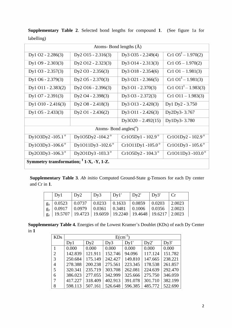
Supplementary Table 2. Selected bond lengths for compound 1. (See figure 1a for

labelling)

Atoms- Bond lengths (Å)

Dy1 O2 - 2.286(3) Dy2 O15 - 2.316(3) Dy3 O35 - 2.249(4) Cr1 O5I – 1.970(2)

Dy1 O9 - 2.303(3) Dy2 O12 - 2.323(3) Dy3 O14 - 2.313(3) Cr1 O5 – 1.970(2)

Dy1 O3 - 2.357(3) Dy2 O3 - 2.356(3) Dy3 O18 - 2.354(6) Cr1 O1 – 1.981(3)

Dy1 O6 - 2.379(3) Dy2 O5 - 2.370(3) Dy3 O21 - 2.366(5) Cr1 O1I – 1.981(3)

Dy1 O11 - 2.383(2) Dy2 O16 - 2.396(3) Dy3 O1 - 2.370(3) Cr1 O11I – 1.983(3)

Dy1 O7 - 2.391(3) Dy2 O4 - 2.398(3) Dy3 O3 - 2.372(3) Cr1 O11 – 1.983(3)

Dy1 O10 - 2.416(3) Dy2 O8 - 2.418(3) Dy3 O13 - 2.420(3) Dy1 Dy2 - 3.750

Dy1 O5 - 2.433(3) Dy2 O1 - 2.436(2) Dy3 O11 - 2.426(3) Dy2Dy3- 3.767

Dy3O20 – 2.492(15) Dy1Dy3- 3.780

Atoms- Bond angles(o)

Dy1O3Dy2 -105.1 o

Dy1O5Dy2 -104.2 o

Cr1O5Dy1 - 102.9 o

Cr1O1Dy2 - 102.9 o

Dy1O3Dy3 -106.6 o

Dy1O11Dy3 -102.6 o

Cr1O11Dy1 -105.0 o

Cr1O1Dy3 - 105.6 o

Dy2O3Dy3 -106.3 o

Dy2O1Dy3 -103.3 o

Cr1O5Dy2 - 104.3 o

Cr1O11Dy3 -103.0 o

Symmetry transformation; I 1-X, -Y, 1-Z.

Supplementary Table 3. Ab initio Computed Ground-State g-Tensors for each Dy center

and Cr in 1.

Supplementary Table 4. Energies of the Lowest Kramer’s Doublet (KDs) of each Dy Center

in 1

Dy1 Dy2 Dy3 Dy1' Dy2' Dy3' Cr

gx

gy

gz

0.0523

0.0917

19.5707

0.0737

0.0979

19.4723

0.0233

0.0361

19.6059

0.1633

0.3481

19.2240

0.0859

0.1006

19.4648

0.0203

0.0356

19.6217

2.0023

2.0023

2.0023

KDs E(cm-1

)

Dy1 Dy2 Dy3 Dy1' Dy2' Dy3'

1

2

3

4

5

6

7

8

0.000

142.839

250.684

278.388

320.341

386.023

417.227

598.113

0.000

121.911

175.149

200.238

235.719

277.055

318.409

507.161

0.000

152.746

242.427

275.561

303.708

342.999

402.913

526.648

0.000

94.096

149.810

223.345

262.081

325.666

391.078

596.385

0.000

117.124

147.665

178.538

224.639

275.750

301.710

485.772

0.000

151.782

238.221

261.857

292.470

346.059

382.199

522.690

3

Supplementary Table 5. RASSI energies of the lowest spin-orbit states (cm-1

) on each Dy

center in complex 1.

Dy1 Dy2 Dy3 Dy1' Dy2' Dy3'

0.000

142.839

250.684

278.388

320.341

386.023

417.227

598.113

3064.645

3175.816

3245.406

3279.445

3310.145

3347.817

3465.300

5678.787

5771.359

5816.455

5866.429

5910.047

6002.422

7881.448

7951.903

8010.601

8069.725

8160.215

9615.778

9659.671

9699.321

9720.235

9746.063

9764.997

9780.431

9817.463

9858.276

9960.088

11033.571

11196.953

11334.515

11861.748

11902.901

11928.297

11939.214

11979.201

13638.669

13674.222

0.000

121.911

175.149

200.238

235.719

277.055

318.409

507.161

3054.606

3126.183

3165.332

3193.872

3233.799

3267.797

3357.391

5660.257

5699.632

5744.679

5789.886

5837.681

5896.043

7846.890

7890.696

7930.615

7998.624

8062.117

9566.384

9603.227

9632.596

9649.181

9676.165

9687.892

9713.287

9742.849

9777.402

9859.809

11000.679

11106.654

11245.606

11792.368

11841.188

11847.554

11864.172

11898.279

13572.873

13594.818

0.000

152.746

242.427

275.561

303.708

342.999

402.913

526.648

3074.156

3174.608

3218.460

3258.765

3294.038

3337.611

3400.436

5697.522

5749.368

5791.126

5843.186

5897.265

5955.957

7895.647

7933.847

7977.075

8050.248

8126.159

9604.569

9652.642

9689.991

9711.924

9724.393

9739.871

9759.978

9782.707

9827.070

9923.271

11036.767

11180.450

11289.242

11846.713

11886.334

11899.434

11909.833

11954.724

13624.016

13646.290

0.000

94.096

149.810

223.345

262.081

325.666

391.078

596.385

3050.378

3118.981

3167.958

3205.075

3260.013

3346.586

3443.568

5649.267

5701.544

5760.421

5793.518

5908.725

5978.470

7835.582

7892.077

7944.348

8057.531

8131.445

9564.374

9615.078

9641.403

9667.293

9699.030

9723.434

9757.407

9793.183

9829.222

9933.927

10998.193

11120.425

11321.904

11811.576

11869.016

11896.181

11909.159

11941.381

13601.627

13630.281

0.000

117.124

147.665

178.538

224.639

275.750

301.710

485.772

3051.190

3113.213

3149.631

3185.583

3223.063

3252.106

3333.258

5652.365

5684.735

5738.326

5776.681

5827.193

5870.996

7833.906

7880.401

7922.663

7987.233

8039.733

9558.664

9588.390

9616.922

9635.200

9664.445

9673.999

9702.807

9733.159

9764.845

9839.773

10994.377

11091.518

11227.435

11779.775

11826.413

11834.777

11853.166

11884.328

13559.052

13582.027

0.000

151.782

238.221

261.857

292.470

346.059

382.199

522.690

3071.004

3175.592

3214.018

3250.228

3287.395

3324.939

3390.684

5691.543

5745.745

5786.778

5838.672

5892.065

5941.873

7885.779

7929.269

7978.407

8044.634

8113.269

9602.403

9642.564

9682.620

9702.083

9717.041

9734.785

9756.172

9782.209

9822.335

9912.372

11035.968

11169.149

11282.283

11839.546

11879.797

11893.337

11906.234

11948.386

13616.914

13640.367

4

Supplementary Table 6. The g-tensors for the eight lowest Kramer’s doublets in 1.

Kramer’s

doublet

Dy1 Dy2 Dy3 Dy1' Dy2' Dy3'

1 gx

gy

gz

0.0523

0.0917

19.5707

0.0737

0.0979

19.4723

0.0233

0.0361

19.6059

0.1633

0.3481

19.2240

0.0859

0.1006

19.4648

0.0203

0.0356

19.6217

2 gx

gy

gz

0.6831

0.8836

16.1314

0.8211

1.3395

15.5887

0.3570

0.4520

16.4132

0.8364

1.5092

15.4053

1.2016

1.8258

15.2248

0.5042

0.5767

16.3829

3 gx

gy

gz

1.1077

1.9123

12.8316

0.1012

0.9926

17.5449

0.1905

0.3842

18.8231

0.0617

2.4196

12.4304

0.3731

1.1095

18.5865

0.4879

1.6275

17.2343

4 gx

gy

gz

0.1593

1.6854

14.6884

2.8806

5.1992

12.7703

2.6274

4.8073

10.6397

1.8987

2.7027

14.2155

1.8359

4.5456

12.4248

1.6378

3.6599

11.9202

5 gx

gy

gz

3.2954

4.3043

12.5431

9.2914

5.7892

0.4029

1.1275

5.0367

10.7298

7.7357

6.1907

1.1361

10.3423

6.2609

2.0397

7.9888

6.1581

1.1761

6 gx

gy

gz

2.7288

3.6217

8.9464

2.0542

3.1486

14.7278

4.2213

4.9437

12.5575

2.3451

4.1734

13.9135

0.6258

2.8863

14.9129

3.0369

5.4057

12.5247

7 gx

gy

gz

11.5008

7.2732

1.3588

0.2936

0.6093

16.6584

0.2485

0.3376

16.9158

0.6471

1.3238

15.4589

0.7873

1.6752

15.7159

0.8622

1.5110

15.8093

8 gx

gy

gz

0.0094

0.0096

19.6474

0.0232

0.0351

19.6861

0.0443

0.0588

19.3823

0.0099

0.2079

19.3655

0.0227

0.0391

19.6361

0.0204

0.03071

19.4563

13734.400

13748.747

15047.530

15083.585

15115.909

16067.481

16082.527

16669.422

38863.904

38937.837

39010.032

39156.925

40254.710

40407.315

40578.827

13661.189

13675.642

14974.830

15009.079

15045.029

15996.096

16008.426

16595.597

38833.695

38904.879

38958.100

39037.093

40221.513

40321.102

40467.096

13709.497

13726.917

15024.607

15062.187

15093.551

16046.066

16058.870

16645.969

38861.673

38938.881

38999.528

39100.134

40250.799

40368.702

40534.439

13693.054

13720.403

15008.672

15047.116

15077.880

16026.753

16047.196

16631.710

38819.623

38923.555

39002.845

39090.914

40217.950

40339.587

40578.249

13648.660

13662.561

14961.272

14996.104

15032.269

15983.326

15995.020

16582.338

38830.762

38893.405

38942.365

39022.341

40215.172

40313.853

40440.300

13704.201

13721.190

15018.016

15056.314

15087.866

16040.107

16052.782

16639.881

38863.948

38933.232

38991.282

39095.137

40249.859

40369.508

40517.090

5

Supplementary Figure 1. Packing diagram of compound 1, with views along the

crystallographic a) a axis b) b axis, c) c axis and d) a highlights the intermolecular

interactions between a neighbouring pair.

a)

b)

c)

d)

6

Supplementary Figure 2. Plots of (left) M versus H isotherms for complex 1 at 2, 3, and 4

K.

Supplementary Figure 3. Plot of χM″ versus T at the frequencies indicated for 1 with;

(left)Hdc = 0 Oe and (right) Hdc = 2000 Oe. The negative value of χM″ are due to instrumental

error for values near to zero.

7

Supplementary Figure 4. Single-crystal magnetization (M) vs. applied field measurements

(μ-squid) for complex 1 at (left) 0.03 K to 0.8 K with the scan rate of 0.14 Ts-1

; and (b) with

different field sweep rates at 0.03 K. The orientation of the magnetic field is shown below.

Supplementary Figure 5. The structure of the modelled Dy fragment employed for

calculation (green, DyIII

; Dark blue, LuIII

, violet, ScIII

).

B

8

Supplementary Note 1. EPR simulation details.

Ab initio computed SINGLE_ANISO results of Dy1, Dy2 and Dy3 are employed as such

along with the J values obtained from the simulation of susceptibility and magnetization data

(see Supplementary Table 3 for the g-tensors and main text for the Js). We have employed

only a {Dy3Cr} model with a pseudo S = 1/2 state for each DyIII

ion and a S = 3/2 state for

CrIII

ion for the simulation. Calculations with full model employing {CrDy6} was not

possible as the system size is very large. The (, ) angles for the Dy-Dy employed are

(63.3,14.9), (53.2,1.2) and (60.2,7.2) for Dy1-Dy2, Dy2-Dy3 and Dy1-Dy3 pair respectively

as obtained from the calculations. Similarly (, ) angles of (45.4,0.0), (60.5,0.0) and

(4.7,0.0) is employed for Cr1-Dy1, Cr1-Dy2 and Cr1-Dy3 pairs respectively. A Gaussian

Line width of 150 G is utilized. The exchange Hamiltonian employed is described in equation

2 in the main text, except that only {Dy3Cr} model is employed for the calculation.

Supplementary Note 2. Single-ion relaxation mechanism

A qualitative mechanism for the magnetic relaxation originating from the Dy1 site, obtained

from the ab initio calculations, is shown in Supplementary Fig. 6 (see below). For all three

DyIII

ions the ground state tunneling probability is computed to be small (for example 0.24

x10-1

for Dy1) suggesting magnetization blockage occurs at the individual ion sites with a

possible relaxation mechanism occurring via the first excited state through a thermally

assisted quantum tunneling of the magnetization (TA-QTM) process. This qualitative

mechanism yields information only about the possible QTM and TA-QTM processes while

other possible relaxations such as the Raman process, deriving from intra/intermolecular

interactions, nuclear-spins of the DyIII

ion and the ligand, spin-lattice relaxation, etc., are not

taken in to consideration. Although this mechanism explains the presence of the low

temperature out-of-phase signals at zero-field, the nature of the '' signals are similar when a

2000 Oe static dc field was applied and the computed barrier heights are much larger than

that observed in the ac susceptibility measurements. This suggests that other factors are

involved and the magnetic blocking does not arise simply from the single ion DyIII

anisotropy.

9

Supplementary Figure 6. The ab initio computed magnetization blocking barrier for a) the

Dy1 site, b) the Dy2 site and c) the Dy3 site. The thick black line indicates the Kramers

doublet (KDs) as a function of computed magnetic moment. The green/blue arrows show the

possible pathway via Orbach/Raman relaxation. The dotted red lines represent the presence

of QTM/TA-QTM between the connecting pairs. The numbers provided at each arrow are the

mean absolute value for the corresponding matrix element of transition magnetic moment.

b) c)

a)

10

Supplementary note 3. How does our analysis of the experimental results exclude a non-

toroidal arrangement?

To probe the robustness of our conclusion i.e. that the ground state in our system is

ferrotoroidically coupled, we varied one of the key results of our CASSCF-RASSI-SO

calculations, which plays a crucial role in determining the ferrotoroidic ground state, namely

the direction of the local anisotropy axes of the Dy ions, and used the resulting modified

model to simulate the experimental magnetization. From our calculations the local anisotropy

axes turn out to be almost exactly contained in the two triangles’ planes, and directed along

the local tangent to the wheel’s circumference. To set up models that depart from this ab

initio result, we generalized our exchange + dipolar coupling Hamiltonian introducing two

angles: an angle measuring the departure of the anisotropy axis from an in-plane

configuration, and an angle measuring the departure of the in-plane projection of the

anisotropy axis from a locally tangential direction. To comply with the D3d pseudo-symmetry

of the metal core of the complex, we demanded that the angle be the same for all Dy ions,

while the angle should have opposite signs for the two wheels, due to inversion symmetry.

We explored two significant scenarios departing from our parameter-free ab initio model, and

reported the resulting powder magnetization curves obtained at 2 K in the figure below,

together with the results of our parameter-free ab initio model (orange curve in the picture)

and the experimental data points (blue data points in the picture):

(i) = 30°, = 0°, i.e. a significant departure from in-plane tangential configuration of the

magnetic axes, which will determine a significant out-of-plane magnetic moment for the

Antiferrotoroidic (AFT) configuration only, but a zero out-of-plane magnetic moment for the

Ferrotoroidic (FT) configuration. Such out-of-plane magnetic component of the AFT state

will also be coupled antiferromagnetically to the Cr magnetic moment, thus stabilizing the

AFT with respect to the non-magnetic FT state. For = 30°, the appearance of a significant

anisotropic out-of-plane magnetic moment in the AFT state, determines a strong Cr-Dy6

antiferromagnetic stabilisation energy contribution which makes the AFT configuration the

ground state, and the FT state the first excited state. However, the powder magnetization we

calculate in this scenario is reported in the picture below (green curve), and evidently it does

not match the experimental data, which instead support our finding that at low field the only

source of magnetic response comes from the Cr ion. Any additional (anisotropic) magnetism

from the Dy-triangles would make the low-field magnetization steeper than what is observed

11

experimentally, which supports our finding of the FT configuration (implying a zero

magnetic moment on the wheels) as the ground state.

(ii) = 0°, = 90°, i.e. the axes are still perfectly in-plane (contained in the planes defined by

the two triangles), but they are now directed radially instead of tangentially to the triangle’s

circumference. In such configuration it is still possible to achieve a non-magnetic non-

collinear ground state on the Dy wheels, for which the magnetism solely arises from isotropic

paramagnetic Cr. However, as first pointed out by some of us1 in radially configured

anisotropy axes, pure dipolar coupling does not favour such non-collinear non-magnetic

configuration of the Dy magnetic moments, and favours instead a large in-plane magnetic

moment in the ground state of each wheel. Furthermore, antiferromagnetic coupling to Cr ion

determines the ferromagnetically coupled state (i.e. the state where the in-plane magnetic

moments of the two Dy triangles lie parallel to each other) as the ground state, so that in fact

adopting a radial instead of a tangential configuration of the magnetic axes leads to a strongly

magnetic and strongly in-plane anisotropic ground state, while the states in which the two

triangles have zero magnetic moment are the highest in energy. This simple rotation of the

Dy anisotropy axes, still compliant with the system’s pseudo-symmetry, and still allowing for

the existence of non-magnetic states on the Dy triangular wheels, leads to a dramatically

different exchange and dipolar coupled spectrum for CrDy6 complex from the FT ground

state predicted by our parameter-free model. However, due to the large and strongly

anisotropic magnetism arising from this scenario, the low-field powder magnetization is in

fact dramatically different from that experimentally observed, as can be seen from its plot in

the figure below (red curve). This model also suggests that the ab initio calculations

accurately reproduce the direction of the local anisotropy axes as in-plane tangential, thus

stabilizing a ferrotoroidic ground state in which the magnetism solely arises from the Cr spin.

We believe that this extended model, together with the fact that our proposed model is

parameter-free, only relying on experimental information (i.e. geometry of complex) and ab

initio calculations, provide strong evidence that the ground state of the title compound CrDy6

is indeed ferrotoroidically coupled.

Furthermore in the new revised version we introduce a substantial extension of our discussion

of the dynamics of the magnetization in this system as observed from the single crystal

magnetization experiments also introducing a theoretical model of the spin dynamics based

on our model Hamiltonian which allows us to simulate and reproduce the zero-field

12

hysteretic magnetic response observed in the experiments This point is further discussed

below but we believe it provides further evidence for the validity of our conclusions

13

Supplementary Figure 7. Measured M vs H for complex 1 (dots) and the theoretical M vs H

plot obtained from the model described in the text (solid line).

14

Supplementary Figure 8. Graphical representation of the states of CrDy6 that are stabilized

by a magnetic field contained in the plane of the figure, and oriented from bottom to top. The

blue (red) arrows at the vertices of the top (bottom) triangle atomic positions represent the

local Dy3+

magnetic moment in that state, while the central yellow arrow represents the Cr

magnetic moment. The blue (red) thin arrows lying above the molecular system in panels c)

and d) represent the direction of a total magnetic moment of ~20 mB arising from the sum of

the Dy3+

atomic magnetic moments belonging to the top (bottom) triangle. Note that only in

the ferrotoroidic states in panel a) and antiferrotoroidic states in panel b) the Cr magnetic

moment is oriented along the field, while in the other states due to Dy-Cr antiferromagnetic

coupling the Cr magnetic moment is oriented opposite to the magnetic field.

15

Supplementary Note 4. Comparison of toroidal coupling in CrDy6 and other Dy6

complexes.

The coupling of two or more triangular Dy3 rings, each stabilizing a toroidal moment in their

ground state, into a structure presenting new collective magnetic properties has been

previously explored in three important works:

1) The earliest work on a Dy6 cluster (Dy6-1) composed of magnetically coupled triangular

subunits is that by Hewitt et al.,2 who achieved a Dy6-1 SMM composed of two co-parallel

but non co-planar triangles, each characterized by uniaxial Dy ions with anisotropy axes

quasi-tangentially arranged around the triangles’ circumference, and characterized by an

inter-triangle antiferromagnetic coupling via two neighbouring vertices. As already pointed

out by Lin et al.3 the work of Hewitt et al.,

2 nicely shows how coupling between toroidal

states can offer new mechanisms to enhance slow magnetic relaxation, although due to the

particular geometry of coupling achieved in that system, the total toroidal moment of Dy6-1 is

not maximized by such coupling, as the antiferromagnetic inter-wheel interaction is such as

to cancel the contribution from the Dy magnetic moment of the two coupled vertices to the

overall vortex magnetisation. In the system we present here the ferrotoroidic ground state

implies on the other hand a maximization of the toroidal moment achievable by six Dy ions.

The nature of the low-energy states in Dy6-1 were indeed graphically represented in the

supplementary information file in terms of con-rotating and counter-rotating toroidal

moments on the two triangular subunits, although the ferrotoroidic and/or antiferrotoroidic

nature of such states was not explicitly discussed, or even mentioned in the main text of the

paper. Given that ferrotoroidic and antiferrotoroidic states are non-magnetic (or weakly

magnetic due to deviation from co-planarity of the Dy anisotropy axes), hence they make

little contribution to the magnetic response of the system, at this stage where no direct

experimental technique can easily probe the toroidal character and relative energy ordering of

con-rotating and counter-rotating toroidal states, it is essential to minimize the source of free

parameters in the theoretical models used to characterized them. In this respect, the fact that

the Hamiltonian used by Hewitt et al. in their work contains four fitting parameters, and

neglects dipolar coupling, suggests that more detailed investigations of Dy6-1 are necessary

to make definitive statements about the ferrotoroidic nature of its ground state. We note here

that the model Hamiltonian used here to simulate the magnetic data for CrDy6 includes

16

dipolar coupling (which in fact is shown to dominate the resulting energy spectrum), and

contains no fitting parameter.

2) Lin et al.,3 have presented an interesting study of a Dy6-2 cluster that can be viewed as two

very closely spaced Dy3 triangular units with two edges, one from each triangle, directly

facing each other. The system is not exactly co-planar, but displays a 29º dihedral angle

between the two triangles’ planes. In that work the magnetic coupling is modeled including

both dipolar and exchange coupling, and the number of free parameters is greatly reduced

with respect to the Hamiltonian reported by Hewitt et al., i.e. Lin et al. only use one fitting

parameter.

We note however that there are a few features of the Hamiltonian used in that paper that

would seem to need further testing before the conclusions drawn about the nature of the

ground state be unambiguously confirmed. First of all, we note that the choice of a single

exchange coupling parameter, especially given that this is a fitting parameter not derived

from a theoretical model or an ab initio calculation, can be in principle criticized. In

particular, we note that while antiferromagnetic coupling between ions belonging to the same

triangle is known to stabilize a toroidal moment, given the geometry of Dy6-2,

antiferromagnetic coupling between nearest neighbor ions on different triangles (e.g. Dy1 and

Dy2 in Fig. S1 of that paper) will in fact stabilize counter-rotating toroidal states on different

triangles, hence an antiferrotoroidic ground state. Given that the distance between Dy1 and

Dy2 in Fig. S1 is shorter (3.34 Å) than any intra-triangular Dy-Dy distance (3.39Å, 3.51Å,

3.54Å), it could be argued that a stronger inter-molecular antiferromagnetic exchange

between such ions could flip the energetic order of the con-rotating and counter-rotating

coupled-toroidal states. On the other hand, an antiferromagnetic diagonal interaction (e.g.

between Dy1-Dy3 in Fig. S1 of that paper) will indeed stabilize a con-rotating toroidal

configuration, but the distance between the Dy ions is in CrDy6 (1) much longer, thus

weakening such interaction (Dy1-Dy3 distance is 4.7Å). Such important competing effects are

clearly not captured by a single fitting parameter, and these issues are not discussed by Lin et

al.3 (We present alternative calculations on Dy6-2 and these are discussed below).

Aside from the details of the Hamiltonian parameterisation, assuming that the arrangement of

local Dy magnetic moments in the ground state of Dy6-2 leads to a maximization of the

overall toroidal moment of the molecule, to characterize such ground state as a

ferrotoroidically-coupled state still seems somewhat problematic on the grounds of two

17

issues, which are in fact related to each other: (i) the triangle-triangle distance is shorter than

two of the intra-triangle’s Dy-Dy distances, so that the detailed connectivity of the central

Dy4 skewed rectangle is bound to play a central role in determining the final magnetic

configuration of the system. This fact poses questions as to whether it is possible to identify

the large toroidal moment in the ground state as resulting from the coupling of two well-

defined separate toroidal subunits, or rather as an overall Dy6 perimeter toroidal arrangement

of magnetic moments resulting from the detailed molecular connectivity of this cluster, that

cannot be simply analysed solely in terms of separate triangular subunits (ii) as a

consequence, assuming the model with a single exchange coupling parameter presented by

Lin et al.3 is valid, the excited putative antiferrotoroidic state in which the toroidal moment

on one triangle is counter-rotating with respect to the toroidal moment on the second triangle

lies in fact at a relatively high energy, at the same energy in fact as that of purely magnetic

excitations not determined by the simultaneous flipping of the spins on all Dy belonging to

one triangular subunit. The lack of low-lying antiferrotoroidic excitations (or rather, the

effective energetic equivalence of toroidal excitations and magnetic excitations), renders this

system a somewhat less clear cut case of a well-defined magnetic coupling between separate

toroidal subunits such as the case presented in this paper, albeit an interesting example of

how to achieve a large toroidal moment in the ground state.

3) Novitchi et al.4 reported the first example of exchange coupling between toroidal moments

in a chiral heterometallic CuII/Dy

III polymer, built from alternating Dy3 SMM building

blocks. The ground state of such system has been found to be antiferrotoroidic, and it is

argued there that the ferrotoroidic first excited state, having a magnetic component, can be

stabilized by magnetic field, so that in a magnetic field applied in the appropriate direction

the ground state would become ferrotoroidic (but not degenerate).

These previous works, and a tutorial review of these works by Tang et al.,5 unveil crucial

information concerning microscopic pathways to the coupling of molecular toroidal

moments, in addition to discussing how to harness the resulting states to enhance SMM slow

relaxation properties (Dy6-1, Hewitt et al.), and to enhance the overall toroidal moment of a

single molecule (Dy6-2, Lin et al.).

Nevertheless, to the best of our knowledge, the CrDy6(1) system presented here, according to

our parameters-free model, provides the first example of a well-defined ferrotoroidic ground

state resulting from the coupling of two separate toroidal subunits, maximizing the total

18

toroidal moment, and characterized by low-lying pure toroidal excitations to antiferrotoroidic

states (counter-rotating toroidal moments resulting in zero toroidal moment), well separated

from higher-energy magnetic excitations.

Alternative calculations on Dy6-2 complex: To test alternative scenarios for Dy6-2 we have

set up an approximate model Hamiltonian in which the two triangles are considered

equilateral using average experimental bond distances, the 29º dihedral angle between the

two triangles’ planes is explicitly taken into consideration, and the deviation from co-

planarity of the Dy anisotropy axes is also included in the model using the data reported in

that paper. Dipolar coupling is explicitly included in the model as is exchange coupling (see

equation 1 in the main manuscript for the dipolar Hamiltonian). However, we introduce here

additional exchange coupling constants to differentiate between intra-triangle coupling, and

the two independent inter-triangle coupling pathways. To illustrate our point, with no

ambition to find optimal fitting parameters in a model that would become quickly over

parameterised, we used our Hamiltonian to simulate the experimental data presented by Lin

et al. (digitalized from paper), both (i) using a single exchange coupling parameter JLin as

reported by Lin et al. thus reproducing their results, and (ii) by setting to zero the diagonal

exchange coupling between the distant cross-coupled ions 4.7Å apart (Jdiag=0), and using two

different constants, one describing intramolecular coupling (Jintra = 1.8 JLin) and

intermolecular coupling (Jinter = 1.5 JLin). The resulting spectra and states are reported in

Supplementary Fig. 9, together with the simulation of the low-temperature (2 K) powder

magnetization compared for the two models (orange curve describes the model of Lin et al,

the green curve is associated to the parameters discussed above). It can be seen that the

simulation of the experimental data is hardly changed in the two settings, but for a single

parameter the ground state consists of con-rotating toroidal states separated by a large energy

gap from the counter-rotating toroidal state (transition indicated with a blue arrow in

Supplementary Fig. 9), almost at the same energy as the first magnetic excitation (transition

indicated with a red arrow in Supplementary Fig. 9), while with the new parameters tried here

the con-rotating and counter-rotating energy ordering is inverted, and the toroidal excitation

is much smaller than the magnetic excitation.

19

Supplementary Figure 9. The energy spectra (cm-1

) and schematic representation of the Dy

ion magnetic moment arrangement in the low-lying collective magnetic states for the the

molecule Dy6-2, modeled using the Hamiltonian reported with parameters (i) Jintra = Jinter =

Jdiago = JLin = -0.2349 cm-1

, i.e. essentially the model reported in Lin et al. (spectrum on the

left), and (ii) Jintra = 1.8 JLin, Jinter = 1.5 JLin, Jdiago = 0.0 (spectrum on the right). The

transitions between ground and lowest lying excited states are indicated with a red (blue)

arrow if the excitation is magnetic (toroidal) in nature. In the top part of the figure a

simulation of the powder magnetization at temperature T = 1.9 K is reported, obtained using

either model (i) i.e. the Lin et al. one-parameter model (green curve), or the three-exchange

parameters model (ii) discussed above (orange curve), together with the experimental data

(blue data points) digitalized from Ref. Lin et al.3

20

Supplementary Figure 10. Energy levels of CrDy6 as function of magnetic field (Zeeman spectrum)

computed using the parameter-free theoretical model presented in the text, but retaining only those 56

states out of 256 that have magnetic anisotropy axes oriented along the y-axis in Figure 6 (easy-axis),

along which the sweeping field of the single-crystal experiment is oriented. These are the 56 states

we have retained in our dynamical model Equation (11).

Supplementary Note 5. Further analysis of the theoretical dynamical magnetization

To further analyse our simulation of the dynamical magnetization, we report the plots of the

contributions to Tr arising from the ferrotoroidic and antiferrotoroidic states

(Supplementary Figure 11(b)), and from the intermediate magnetic states and the onion states

(Supplementary Figure 11(c)). It can be seen that the hysteresis loop about the zero field

region is not produced by the free fluctuating paramagnetic Cr spin (in zero field the

magnetization of the FT and AFT states in Supplementary Figure 11(b) is zero), but, as

evident from Supplementary Figure 11(c), the zero-field hysteresis loop arises from the

lagging in the depletion of the non-equilibrium populations of the excited intermediate states

predominantly, with contributions from the onion magnetic states as well. Note also that the

contribution of FT states to the dynamics is visibly much larger than that of the AFT states.

Finally, we note that, due to the choice of coupling constants, the dynamics portrayed in

Supplementary Figure 11 is dominated by the 1-flip transitions, as evidenced by the fact that

the magnetization at high fields is dominated by the excited intermediate states (see

Supplementary Fig. 11(c)). If we now solve Equation (8)/ Equation (11) for a slightly

different set of parameters, still preserving the proposed hierarchy, but using faster 2-flip

transitions, so that Cr = 3 104 Hz/(cm-1)3>>1 = 3.33 10-7 Cr>2 = 10-2

1 , and Cr =

41015 Hz2>>1 = 2 1012 Hz2>2 = 10-11, we obtain a hysteretic magnetization reported in

Supplementary Figure 12(a), which still reproduces the zero-field hysteresis loop, with an

21

almost closed hysteresis at high fields, but now dominated by the onion states at high fields

(see Supplementary Figure 12(c)), and displaying a sizeable contribution from AFT states at

low-fields, almost as large as that of the FT states (see Supplementary Figure 12(b)), but

otherwise not changing the main conclusions drawn above.

Supplementary Figure 11. a) Single-crystal experimental magnetization (blue curve) measured at T

= 0.03 K and a sweep rate of 0.1T/s for a magnetic field oriented parallel to the triangles’ planes and

along the easy-axis (y axis in Figure 6), superimposed to the simulated dynamical magnetization at the

same temperature, sweep rate and field orientation, by solving Equation (11)/ Equation (8) on the

basis of 56 out of the 256 states obtained from our model and reported in Supplementary Figure 8, for

the following numerical values of the transition rates appearing in the equations: Cr = 105 Hz/(cm-

1)3>>1 =10-7 Cr>2 = 10-3

1 , and Cr = 1016 Hz2>>1 = 1012 Hz2>2 = 10-31; b) Contribution to the

total simulated dynamical magnetisation reported in panel a) from the ferrotoroidic (blue solid line)

and antiferrotoroidic (orange dashed line); c) Contribution to the total simulated dynamical

22

magnetisation reported in panel a) from the intermediated magnetic states (blue solid line) and onion

states (orange dashed line).

Supplementary Figure 12. a) Single-crystal experimental magnetization (blue curve) measured at T

= 0.03K and a sweep rate of 0.1T/s for a magnetic field oriented parallel to the triangles’ planes and

along the easy-axis, superimposed on the simulated dynamical magnetization at the same temperature,

sweep rate and field orientation, by solving Equation (11) on the basis of 56 out of the 256 states

obtained from our model, for the following values of the transition rates: Cr = 3 104 Hz/(cm-1)3>>1

= 3.33 10-7 Cr>2 = 10-2

1 , and Cr = 41015 Hz2>>1 = 2 1012 Hz2>2 = 10-11; b) Contribution

to the total simulated dynamical magnetisation reported in panel a) from the ferrotoroidic (blue solid

line) and antiferrotoroidic (orange dashed line); c) Contribution to the total simulated dynamical

magnetisation reported in panel a) from the intermediated magnetic states (blue solid line) and onion

states (orange dashed line).

23

Supplementary References

1. Giansiracusa, M. J. et al. Carbonate-Bridged Lanthanoid Triangles: Single-Molecule Magnet

Behavior, Inelastic Neutron Scattering, and Ab Initio Studies. Inorg. Chem. 55, 5201-5214

(2016).

2. Hewitt, I. J. et al. Coupling Dy3 Triangles Enhances Their Slow Magnetic Relaxation. Angew.

Chem. Int. Ed. 49, 6352-6356 (2010).

3. Lin, S.-Y. et al. Coupling Dy3 Triangles to Maximize the Toroidal Moment. Angew. Chem. Int.

Ed. 51, 12767-12771 (2012).

4. Novitchi, G. et al. Heterometallic CuII/Dy

III 1D chiral polymers: chirogenesis and exchange

coupling of toroidal moments in trinuclear Dy3 single molecule magnets. Chem. Sci. 3, 1169-1176

(2012).

5. Ungur, L., Lin, S.-Y., Tang, J. & Chibotaru, L. F. Single-molecule toroics in Ising-type lanthanide

molecular clusters. Chem. Soc. Rev. 43, 6894-6905 (2014).