Credit-Based Congestion Pricing: Travel, Land Value and Welfare Impacts

By

Sukumar Kalmanje

Graduate Student Researcher

The University of Texas at Austin

6.9 E. Cockrell Jr. Hall

Austin, TX 78712-1076

sukumar@mail.utexas.edu

and

Kara M. Kockelman

Clare Boothe Luce Professor of Civil Engineering

The University of Texas at Austin

6.9 E. Cockrell Jr. Hall

Austin, TX 78712-1076

kkockelm@mail.utexas.edu

Phone: 512-471-0210

FAX: 512-475-8744

(Corresponding author)

The following paper is a pre-print and the publication can be found in

Transportation Research Record No. 1864 : 45-53, 2004.

Presented at the 83rd

Annual Meeting of the Transportation Research Board, January 2004

ABSTRACT

This paper explores the possible transportation and property value impacts of a new congestion

management policy called credit-based congestion pricing (CBCP). Using destination, mode and

departure time choice models sensitive to changes in travel times and costs, household travel

demands were simulated in order to appreciate the transportation effects of a CBCP policy for

Austin, Texas. Changes in home values as a result of CBCP also were simulated. The trip-based

welfare impacts of such a policy were compared for three scenarios (full network pricing, major

highway pricing only, and no pricing), in order to identify households and neighborhoods that

will benefit most and least from such policies. The results corroborate prior results and

hypotheses about the potential of a CBCP policy to alleviate congestion and generate benefits

across the region and traveler types.

Key words: Credit-based congestion pricing, travel demand modeling, welfare, property value

models, transportation policy

INTRODUCTION AND OBJECTIVES Users and planners of transportation systems alike have long been grappling with the problem of increasing road congestion. Road congestion is an externality that results in substantial time losses1; and it is no surprise that Americans consistently rank it among the top three regional policy issues, along with education and crime. (See, e.g., Scheibal, 2002, Knickerbocker, 2000 and Fimrite, 2002.) During peak-periods of demand, drivers tend to over-utilize the common road resource without paying for or even noting the associated, marginal costs borne by fellow travelers. As a result, a wide variety of demand management policies (intended to control congestion) have been proposed. Congestion pricing, a popular policy with researchers and economists, (e.g. Vickrey, 1963 and 1969, Arnott et al, 1993, Button and Verhoef, 1998, Small and Yan, 2001) has only recently garnered significant attention by the public and policy makers (e.g., Hyman and Mayhew, 2002, Litman, 2003). Various forms of congestion pricing have been implemented in places like Singapore, London (Litman, 2003), and California (SR-91 and IH-15) (Sullivan et al., 2000), with different degrees of success. Following London’s example, many cities in Europe and the US have been willing to explore CP as a viable travel demand management strategy (see, for example, Zupan and Perrotta, 2003, Deloitte Research, 2003). Congestion pricing (CP) is based on the principle that if people pay the true marginal cost of road use, the congestion externality is internalized and lower but more efficient levels of road use result during peak periods. While there are many advantages to this approach (see, e.g., Vickrey, 1963, and Arnott and Small, 1994), the major criticism has been the adverse equity impacts on low-income groups and others with special travel needs. Alternate pricing methodologies for addressing CP equity issues have been proposed. Dial (1999) made a case for minimum-revenue CP in place of marginal cost CP, Viegas (2001) argued for the creation of “mobility rights” for individuals, Rothengatter (2003) hinted at the possibility of viewing transportation as a club good (in place of a public good) and De Corla-Souza (2000) championed the creation of FAIR (Fast and Intertwined) Lanes. In addition, Daganzo (1995) and Nakamura and Kockelman (2002) explored the possibility of tolls-plus-roadspace rationing as a demand management strategy. To tackle the equity issue, Kockelman and Kalmanje (2003) proposed a revenue-neutral policy called credit-based congestion pricing (CBCP), where tolls generated from marginal cost pricing (MCP) are returned to all licensed drivers in a uniform fashion, as a sort of driving “allowance”. Under CBCP, the “average” driver pays nothing, the below-average driver makes some money, and frequent, long-distance and peak-period drivers pay something out of pocket, in effect paying others to stay off congested roads. As CP gains attention and application, CBCP may provide the most equitable and efficient implementation alternative. Hence, it could be of interest to transportation system planners, policy makers and the public to obtain reliable predictions of travel demand, land use, air quality, property value and welfare impacts of a CBCP policy. Models of these impacts help one appreciate and compare network-wide and corridor-specific alternatives, CBCP and standard marginal-cost CP strategies, and other scenarios. In the short term, there may not be substantial changes in many behaviors and conditions. Many travelers are at least temporarily “locked in” to their places of employment and education, as well as to their residences. In the longer term, however, CBCP could have sizable impacts – and differential impacts, based on demographic and other factors. Hence, it behooves us to predict, analyze and

plan for short- and long-term changes in a variety of behaviors and responses that emerge following implementation of a CBCP policy. Texas’s capital city, Austin, makes a valuable case study for appraising policy impacts. With an annual traffic delay of 61 hours per peak period road traveler, Austin ranks 5th among U.S. cities in terms of congestion cost per person (Schrank and Lomax, 2002). Together with an estimated annual fuel loss of 104 gallons per peak-period road user, year-2000 annual time and fuel costs are estimated to total $1190, per peak-period user2 (Schrank and Lomax, 2002). A recent survey of Austin residents gauged traveler perceptions of and responses to congestion and a hypothetical CBCP policy (Kockelman and Kalmanje, 2003). Population-weighted results of the 580-person sample suggest that 25% of Austin’s driving population would support this new strategy; furthermore, support is strongly, and positively, related to familiarity with the concept of congestion pricing. Thus, education may be key to marketing such policies. While 58.1% of the survey respondents were very concerned with policy implementation issues (i.e., ease of use), 56.2% attached a very high value to fairness or “equity” considerations. Currently, focus group studies are also underway at the University of Texas at Austin, in order to assess perceptions and needs of special groups, such as small business owners. This paper examines network-wide CBCP and major-corridors-only CBCP, and compares the transportation, welfare and property value impacts of these strategies using Austin-calibrated comprehensive models of household travel demand, it evaluates traffic and welfare impacts, based on changing costs to reach different destinations from one’s place of residence, across modes and times of day. Property values of Austin residences also were modeled, in order to anticipate changes in home prices due to CBCP policies, permitting a more holistic view of impacts on the Austin population. DATA SOURCES AND DETAILS The primary sources for calibrating the travel demand models are the 1998-1999 Austin (Household) Travel Survey (ATS 1998) conducted by the Capital Area Metropolitan Planning Organization (CAMPO 2000, 2001). Network travel time and background flow results from the CAMPO model (which were used for air quality conformity analysis of the region’s 2025 Transportation Plan) also were used. Other data sources include the 2000 Census of Population, the 2000 CAMPO-maintained City of Austin land use data set, and 2003 home sales data from the Travis County Appraisal District (TCAD). The Census data provided information on vehicle ownership and income, for calibrating the trip generation models. The land use data facilitated calibration of the generation and attraction models. CAMPO’s network travel time data file has travel time and network distance information for each pair of the 1074 Traffic Assignment Zones (TAZ) in the three-county Austin metropolitan planning region. The data vary by time of day and travel mode3. For the automobile mode, the two-hour morning peak and 24-hour off-peak period travel times were available. For transit, travel times varied by service type (i.e., University of Texas shuttle buses, Capital Metro standard buses and express buses) and transit access (i.e., by walking or driving). Walk/bike travel times were obtained assuming 6 mi/hr travel speeds on the shortest paths between zones. These data were used to calibrate the destination, mode, and departure time choice models.

MODELING FRAMEWORK Travel Demand Model (TDM) Calibration The travel demand models include a destination choice model that captures accessibilities across multiple modes and time periods, and a joint mode-departure time choice model. Trip generation (TG) models were developed for four trip purposes (home-based work, home-based non-work, non-home-based work, and non- home-based non-work trips) in order to better appreciate changes in TG that may occur in the long term under CBCP. Trip productions for home-based trips were modeled at the household level (using the ATS data set) and then aggregated to the zonal level. Trip productions for non-home-based trips and trip attractions were all modeled at the zonal level. The models for TG internal to the region are shown in Table 1. External trip productions and attractions were computed from average daily traffic counts at the external stations. Joint multinomial logit models for mode and time of day were calibrated considering four modes (drive alone, shared ride, transit, and walk/bike) and five time periods (late night and early morning, morning peak, afternoon, evening peak, and evening off-peak periods). The resulting models (for each of the 4 trip purposes) are shown in Table 2.4 The multinomial logit models of destination choice are shown in Table 3. Since the attractiveness of the destination zone varies across mode and time of day, this variability was captured using logsums of travel times, travel costs and alternative-specific constants obtained from the mode-departure time model calibrated earlier. By constraining the coefficient on ln(ATTRj) to equal one, the structure of the destination choice models mimics a gravity model, offering ease of application in TransCAD (Caliper, 2002). The (systematic) utility of a destination from a particular origin is given by equation (1).

)ln()ln( ,,,,,,,, pjpjpspjiplpji ATTRSIZELOGSUMV ++= ββ (1)

where SIZEj is either the area or the employment at the destination zone “j”, ATTRj is the attraction at the destination zone “j”, and LOGSUMi,j is the “logsum” for the origin-destination pair (i, j), computed as shown in equation (2). The logsum is the negative of the expected maximum utility derived across all mode and departure time combinations for that particular destination, and it is a measure of accessibility of that destination from origin of interest (i).

ln - ,

,,,,,,,,

= ∑

++

tm

CostTimepji

ptmjipcjipteLOGSUM βββ (2)

where βt , βc and βm,t are the joint mode-departure time model coefficients (on time, cost and the alternative-specific constants, respectively). The joint mode-departure time model’s coefficients are shown in Table 3. All the multinomial logit models for destination and joint mode and time of day choice were calibrated using GAUSS’s maxlik module (Aptech, 1996).

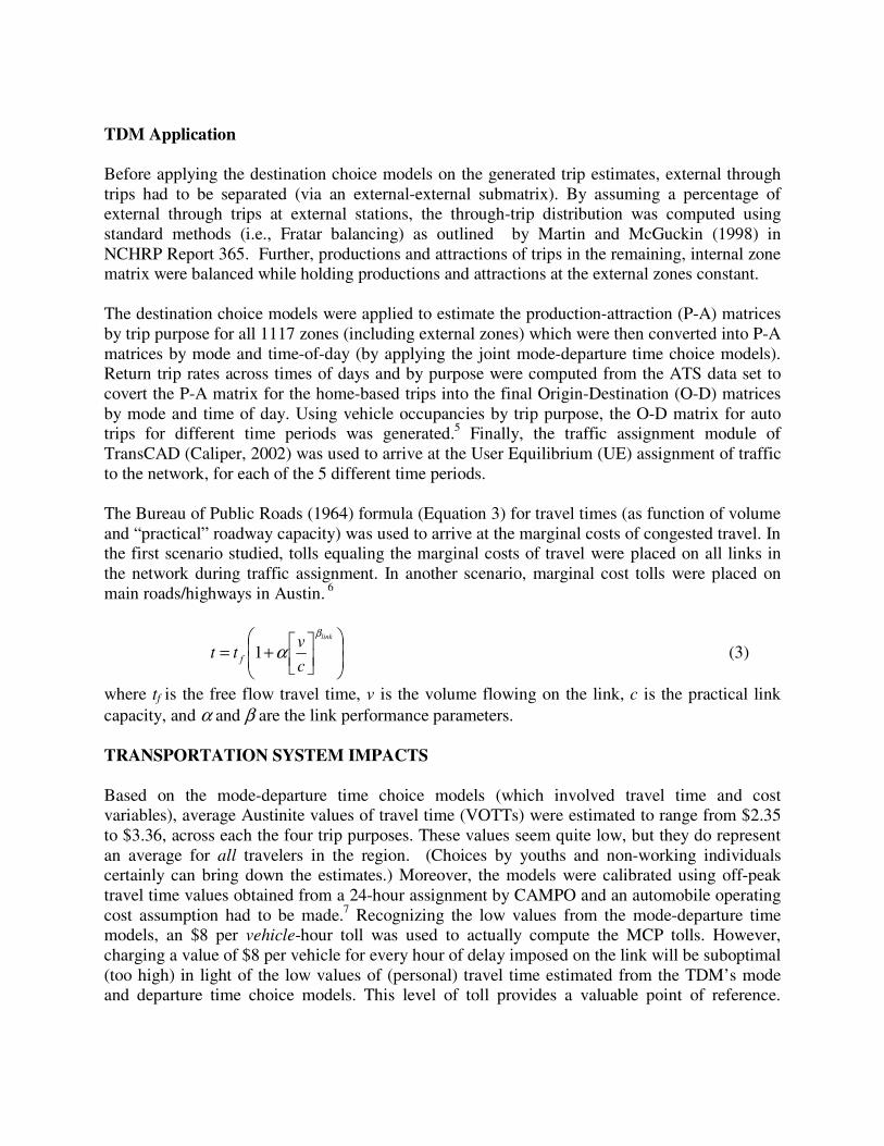
TDM Application Before applying the destination choice models on the generated trip estimates, external through trips had to be separated (via an external-external submatrix). By assuming a percentage of external through trips at external stations, the through-trip distribution was computed using standard methods (i.e., Fratar balancing) as outlined by Martin and McGuckin (1998) in NCHRP Report 365. Further, productions and attractions of trips in the remaining, internal zone matrix were balanced while holding productions and attractions at the external zones constant. The destination choice models were applied to estimate the production-attraction (P-A) matrices by trip purpose for all 1117 zones (including external zones) which were then converted into P-A matrices by mode and time-of-day (by applying the joint mode-departure time choice models). Return trip rates across times of days and by purpose were computed from the ATS data set to covert the P-A matrix for the home-based trips into the final Origin-Destination (O-D) matrices by mode and time of day. Using vehicle occupancies by trip purpose, the O-D matrix for auto trips for different time periods was generated.5 Finally, the traffic assignment module of TransCAD (Caliper, 2002) was used to arrive at the User Equilibrium (UE) assignment of traffic to the network, for each of the 5 different time periods. The Bureau of Public Roads (1964) formula (Equation 3) for travel times (as function of volume and “practical” roadway capacity) was used to arrive at the marginal costs of congested travel. In the first scenario studied, tolls equaling the marginal costs of travel were placed on all links in the network during traffic assignment. In another scenario, marginal cost tolls were placed on main roads/highways in Austin. 6

+=link

c

vtt f

β

α1 (3)

where tf is the free flow travel time, v is the volume flowing on the link, c is the practical link capacity, and α and β are the link performance parameters. TRANSPORTATION SYSTEM IMPACTS Based on the mode-departure time choice models (which involved travel time and cost variables), average Austinite values of travel time (VOTTs) were estimated to range from $2.35 to $3.36, across each the four trip purposes. These values seem quite low, but they do represent an average for all travelers in the region. (Choices by youths and non-working individuals certainly can bring down the estimates.) Moreover, the models were calibrated using off-peak travel time values obtained from a 24-hour assignment by CAMPO and an automobile operating cost assumption had to be made.7 Recognizing the low values from the mode-departure time models, an $8 per vehicle-hour toll was used to actually compute the MCP tolls. However, charging a value of $8 per vehicle for every hour of delay imposed on the link will be suboptimal (too high) in light of the low values of (personal) travel time estimated from the TDM’s mode and departure time choice models. This level of toll provides a valuable point of reference.

However, welfare estimates are biased low as a result. And the resulting MCP tolls are likely to be more severe than optimal, reducing congestion more than necessary. From Table 4 one observes that total revenue generated from the MCP of all roads is around $372,000 per day. As expected, the revenues generated during the off-peak periods are quite small, compared to the peak periods. Under system-wide MCP, it is observed that average peak travel times decreased by roughly 1.6% (3.3% on main roads). The highest tolls arise along the highly congested Interstate 35 (I35) corridor, which carries a great many through (external zone-to-external zone) trip-makers, who cannot be priced off the corridor under present assumptions. Given some assumptions about demand responsiveness on this corridor, the I35 (and average) tolls are likely to fall. There may be considerable implementation costs for CBCP since it requires Electronic Toll Collection (ETC) and other technologies for managing user accounts and enforcement. However, most of the technology and administration needed is similar to that used for CP implementation, and it is anticipated that the costs of implementing CBCP will be a relatively small portion of revenues collected, when undertaken in congested regions (such as Austin). In this paper, we have analyzed scenarios wherein all revenues are returned to the drivers. A certain portion of revenues could be earmarked for making system improvements, reducing gas and other taxes, and/or providing greater transit and parking services which will indirectly improve welfare once again (see, e.g., Parry and Bento, 2001). POLICY IMPACTS ON WELFARE AND PROPERTY VALUES Welfare Impacts of CBCP Those unable to afford the tolls under CP and therefore forced to change trip making substantially are generally perceived as “losers” under conventional CP. Compensation in the form of cash travel credit allowances under CBCP should substantially increase welfare for such people and also for the whole community. Using Schrank and Lomax’s (2002) estimate of 730,000 road users in Austin, the revenue returned by CBCP per user per day comes to around 50¢, if system wide pricing were to be applied, and around 20¢, if MCP applied only to the main roads.8 Under CBCP, this amount is given as a “rebate,” in the form of a monthly allowance. Consumer surplus at the destination choice level after the policy change has been used as the welfare measure in this paper since it provides an excellent holistic/comprehensive measure of impact, capturing impacts on destination, mode and departure time of day choices.9 Equation (4) gives the expression for consumer surplus under a policy change; it is the difference in the expected maximum utilities before and after the policy change. It is based on a given origin, assumed to be one’s neighborhood of residence, and it is computed as a logsum of utilities of all destination choices from that origin with Vi,j,p denoting the utility of person at origin i choosing destination j (see equation 1) for trip purpose p, with C denoting the full choice set of all possible destinations.

( )opij

npij

ppi UMaxEUMaxECS ))(())((

1, −=

α (4)

= ∑

∈Cj

V

pijpjieUMaxE ,,ln))(( (5)

where n and o denotes the new and old policies/environments (i.e., CBCP versus the status quo) and αp is the trip purpose specific destination choice model’s marginal utility of money, in this case equaling the multiple of the coefficients on cost (in the mode-departure time model) and generalized cost or logsum (in the destination choice model). Consumer surplus (CSi,p) under CBCP has been calculated for an average individual located in every zone i for each trip purpose p using the corresponding destination and mode-departure time choice models. The rebate per trip (R) was calculated by dividing the daily allowance by an individual’s daily average number of trips. Average daily trip making of 4.6 trips/individual (from the ATS survey) was assumed to calculate the average CBCP allowance for each trip, and a trip-weighted average of the trip-based welfare measures produced the final measure (CS) shown in equation (6).

∑

∑ +=

pp

pppi RCS

CS#

)*#( ,

(6)

where #p is the average number of trips by each purpose per individual. Results of the welfare analysis for both the CBCP policies tested are shown in Table 5. Figures 1 and 2 illustrate the geographical variation in aggregate consumer surplus around Austin for system-wide CBCP and main-roads-only CBCP. Note that the potential “winners” under these two policies can be very different. While users near the central business district (CBD) are predicted to gain from pricing only the main roads, users living in northwest Austin (close to several major employers) gain the most under system-wide CBCP. Since tolls charged are based on a higher VOTT estimate than those obtained from our model estimates, welfare changes under CBCP for an average Austin resident may be largely (or exclusively) positive throughout the region. Home Sales Price Changes under CP The home sales price model was calibrated using the Travis County Appraisal District’s substantial records of recent home sales prices. The home sales price models recognize that a property’s value depends, in part, on locational accessibility ( see, e.g., Kockelman, 1997, Srour and Kockelman, 2002). Locational accessibility derives from travel times and costs, which are affected by the policies under study. Accessibility’s impact on home value was captured here using the trip generation-weighted average of destination logsums (Equation 5) from the travel demand models, thus effectively quantifying the overall accessibility of the residential location across trip purposes, modes and times of day (see, e.g., Waddell and Nourzad, 2002). The home sales price model estimates are provided in Table 6. The home sales price model was used to predict changes in average home values across Austin locations upon implementing standard CP. Based on predicted values for the median dwelling unit sold in year 2000 (i.e., one that is 1,958 square feet in size and 9 years old) located at zonal

centroids, home values are predicted to fall slightly in almost all areas when all roads are priced (i.e., CP – All Roads). Home values are estimated to fall between 1.5% and 6.4% in southwest Austin, but other regions (including the CBD) are predicted to experience lesser drops. When pricing only major roads (i.e., CP-Main Roads Only), home values again dropped slightly in most areas, but home values in some CBD areas were predicted to actually increase marginally. Figures 3 and 4 show the distribution of price effects across Austin for both pricing scenarios. These predicted price changes are reasonably minor, yet more severe than what would occur under a credit-based CP policy, since credit budgets would offset much of the diminished access effects experienced by neighborhoods whose accessibility logsums fell under standard CP. CONCLUSIONS AND EXTENSIONS Credit-based congestion pricing (CBCP) has the potential to address a variety of redistributive impacts that are likely under congestion pricing policies. This work investigates the travel demand and property value impacts of such a policy, under a variety of pricing scenarios for the Austin, Texas, region. It uses a standard four-step travel demand modeling approach, calibrated on the basis of the most recent Austin Travel Survey (ATS, 1998), and relying on logit models of departure time, mode, and destination. It then applies the policy to the entire network and to main highways at different times of day and at different levels of charges, in order to appreciate the variety of applications and impacts that could arise in practice. The work also examines the impacts of changes in access (due to pricing without credit redistribution) for effects on home property values. The results of the model application to various policy scenarios suggest that most Austin residents would be better off under policies that employ CBCP, whereas relatively few would benefit under a policy of congestion pricing, without beneficial revenue redistribution. Residential property prices are estimated to fall marginally, with some areas near the CBD gaining if CP were implemented on major highways only. Under a CBCP policy, the presence of travel rebates could cause property values to increase much more widely. Realistically, the most likely CBCP policies for Austin or any other region may be a CBCP policy with approximate, relatively stable MCP on all arterial links, thereby providing some price certainty and avoiding overuse of unpriced arterials. Pricing of all network links provides further gains, but the costs (and other impacts) of providing roadside detection (and enforcement) along all such corridors may be prohibitive in the near term. This work may provide the insight that is needed for policymakers, engineers, and economists to take the next step toward application of this promising policy proposal. ACKNOWLEDGEMENTS We wish to thank the Southwest Region University Transportation Center for financially supporting this study, and Sriram Krishnamurthy for his valuable input during every stage of the work. Many thanks to Alex Marks for leading the CBCP focus groups and calibrating initial home value models. Thanks are due to CAMPO’s Daniel Yang, the City of Austin Spatial Analysis Group’s Paul Frank, and Parsons Brinkerhoff’s Karen Smith for assistance in obtaining data and resolving data issues. Thanks also go to Sriharsha Nerella, for useful discussions during different stages of this work.

ENDNOTES 1 Schrank and Lomax (2002) estimated that congestion in 75 major U.S. urban areas in the year 2000 cost the traveling public $68 billion in fuel and time losses. This amounts to an estimated $1,160 average cost per peak-period traveler in those areas. 2 Peak-period users may comprise more than half of the Austin region’s population. Schrank and Lomax (2002) estimate that 60% of person-miles of freeway travel and 65% of arterial miles of travel are made in peak–period, congested conditions. (Schrank and Lomax, 2002). 3 Since the travel time data was not available for different times of day, a joint mode-departure time choice model was used and travel times were obtained based on the resulting traffic assignment. These travel times then fed back to the other models, thus offering more variation in automobile and transit travel times, being based on five (rather than two) times of day. The five times of day are Early morning/Late evening (before 7.15 a.m. and after 8.15 p.m), Morning peak (7.15 to 9.15 a.m.), Noon (9.15 a.m. to 4.15 p.m.), Evening peak (4.15 to 6.15 p.m), and Evening off-peak (6.15 to 8.15 p.m.). 4 Nested logit models of mode and time of day also were attempted, but these specifications refused to converge, regardless of nesting structure and trip type. 5 Average automobile vehicle occupancy varies from 1.18 for home-based work trips to almost 2.0 for non-work auto trips. Vehicle occupancy for automobile “shared ride” trips, which comprise 39% of all person trips made in the Austin region, varies from 2.38 to 2.70. Transit trips were too few to be factored in while computing the automobile-trip matrix . 6 Values of α = 0.15 and β = 4.0 were used in cases where link-specific values were not provided. The final travel times compared favorably with the travel times provided by CAMPO with an average difference of -2% (and a normalized standard deviation of 0.06, or 6%) for off-peak values and -8% (s.d.=11.5%) for peak values. Marginal cost pricing scenarios were applied by altering the volume flow functions for the marginally priced links by replacing the α in the BPR formula with α+β. 7 The travel cost by automobile was assumed to be 30¢/mile, which is probably high, in marginal terms (since most travelers already have access to an insured vehicle and therefore are only considering gasoline and some other variable costs). A higher assumed travel cost, however, will result in a higher VOTT prediction for the model (since the parameter on cost will fall, and the ratio of the time and cost coefficients, the VOTT, will rise). 8 The main roads subject to MCP are US-183 (Research Blvd.), IH-35, Loop 1 (Mopac), Loop 360 (Capital of Texas Highway), Highway 71 (Ben White) and US 290, as specified in Kockelman and Kalmanje’s (2003) surveys of Austinites. 9 The changes in transit level of service under the policies also have been recognized. Transit travel times were adjusted for changes in peak and off-peak travel times under the various policies, according to the shift in the corresponding auto travel times.

REFERENCES

Aptech Systems Inc. (1996). GAUSS Mathematical and Statistical System. Aptech Systems Inc., Maple Valley, Washington

Arnott, R., de Palma, A. and Lindsey, R. (1993). “A Structural Model of Peak-period Congestion: A Traffic Bottleneck with Elastic Demand.” American Economic Review. 83:161-79.

Arnott, R., and Small, K. (1994). “The Economics of Traffic Congestion.” American Scientist. Vol 82: 447-455.

ATS (1998). Austin Travel Study. City of Austin, Austin.

Bureau of Public Roads. (1964). Traffic Assignment Manual. Washington D.C.

Button, K.J. and Verhoef, E.T. (1998). Ed., Road Pricing, Traffic Congestion and the Environment: Issues of Efficiency and Social Feasibility. Edward Elgar, Cheltenham.

CAMPO (2000). 1997 Base Year Travel Demand Model Calibration Summary for Updating the 2025 Long Range Plan. Transportation Planning and Programming Division, TXDOT.

CAMPO (2001). CAMPO Mode Choice Model Application Draft. Capital Area Metropolitan Planning Organization, Austin.

Caliper Corporation (2002). Travel Demand Modeling with TransCAD 4.5. Caliper Corporation, Newton, Massachusetts.

Daganzo, C. (1995). “A Pareto Optimum Congestion Reduction Scheme.” Transportation Research. B(29):139-154.

DeCorla-Souza, Patrick. (2000). “FAIR lanes: A New Approach to Managing Traffic Congestion.” ITS Quarterly, Vol. VIII, No.2

Deloitte Research (2003). Combating Gridlock: How Pricing Road Use can Ease Congestion. Deloitte Research, NY. Accessed from http://www.deloitte.com/dtt/cda/doc/content/dtt_research_Gridlock_110303.pdf (Nov, 10, 2003).

De Palma, A., and Lindsey, R. (2002). “Road Pricing for a Simple Monocentric City with a Radial Network.” Presented at the 49th Annual North American Meetings of the Regional Science Association International, San Juan, Puerto Rico, November 14, 2002.

Dial, R.B. (1999). “Minimal Revenue Congestion Pricing Part I: A Fast Algorithm for the Single-Origin Case.” Transportation Research. B(33):189-202.

FHWA (1993). Employer-Based Travel Demand Management Programs - Guidance Manual. Federal Highway Administration

Fimrite, P. (2002), “Traffic Tops List of Bay Area Banes, Weak Economy is Number 2 Bane, Survey Shows.” San Francisco Chronicle. Accessed from http://sfgate.com/cgi-bin/article.cgi?file=/c/a/2002/12/05/MN51835.DTL#sections (5, Dec. 2002).

Hyman, G. and Mayhew, L. (2002)/ “Optimizing the benefits of Road User Charging.” Transport Policy. 9:189-207.

Knickerbocker, Brad. (2000). “Forget Crime - but Please Fix the Traffic.” Christian Science Monitor. (February 16)

Kockelman, Kara (1997). “The Effects of Location Elements on Home Purchase Prices and Rents.” Transportation Research Record. No. 1606: 40-50.

Kockelman, K., and Kalmanje, S. (2003). “Credit-Based Congestion Pricing: A Policy Proposal and the Public’s Response.” To be presented at the 10th International Conference on Travel Behaviour Research (Lucerne, Switzerland, 10-14 August 2003) and submitted to Transport Policy.

Krishnamurthy, Sriram (2002). Master’s Thesis. University of Texas at Austin.

Krishnamurthy, S. and Kockelman, K. (2003). “Propagation of Uncertainty in Transportation-Land Use Models: An Investigation of DRAM-EMPAL and UTTP Predictions in Austin, Texas.” Forthcoming in Transportation Research Record (2003), and presented at the Transportation Research Board's 82nd Annual Meeting (2003).

Litman, T. (2003). “London Congestion Pricing: Implications for Other Cities.” Victoria Transport Policy Institute. Victoria, BC, Canada. http://www.vtpi.org/london.pdf (Accessed on 7th July 2003).

Martin, William. A., and McGuckin, Nancy A. (1998). Travel Estimation Techniques for Urban Planning. NCHRP Report 365. National Research Council, D.C.

Nakamura, K., and Kockelman, K. (2002). “Congestion Pricing & Roadspace Rationing: An Application to the San Francisco Bay Bridge Corridor.” Transportation Research A. 36(5): 403-417.

Parry, I.W.H and Bento, A. (2001). “Revenue Recycling and the Welfare Effects of Road Pricing.” Scandinavian Journal of Economics. 103(4):645-671.

Poole, R.W., and Orski, C.K. (2003). HOT Networks: A New Plan for Congestion Relief and Better Transit. Reason Public Policy Institute.

Rothengatter, W. (2003) “How good is first best? Marginal Cost and Othe Pricing Priciples for User Charging in Transport.” Transport Policy. 10:121-130.

Scheibal, S. (2002). “New Planning Group Kicks-off Effort with Survey on What Area Residents Want.” Austin American Statesman. (26 Aug. 2002)

Schrank, D. and Lomax, T. (2002). The Urban Mobility Report. Texas Transportation Institute, College Station, TX.

Small, K.A. and Yan, J. (2001) The Value of “Value Pricing” of Roads: Second-Best Pricing and Product Differentiation. Journal of Urban Economics. 49:310-336.

Srour, Issam M., Kockelman, Kara M. and Dunn, Travis P. (2002) “Accessibility Indices: A Connection to Residential Land Prices and Location Choices.” Transportation Research Record. No.1805: 25-34.

Sullivan, E., with Bakely, K., Daly, J., Gilpin, J., Mastako, K., Small, K., and Yan, J. (2000) Continuation Study to Evaluate the Impacts of the SR 91 Value-Priced Express Lanes: Final Report. Department of Civil and Environmental Engineering, California Polytechnic State University at San Luis Obispo. Accessed from http://ceenve.ceng.calpoly.edu/sullivan/SR91/

(13, December 2002).Vickrey, W.(1963). “Pricing in Urban and Suburban Transport.” American Economic Review, 52(2):452–465.

Vickrey, W.(1969). “Congestion Theory and Transport Investment.” American Economic Review, 59(2):251–260.

Viegas, J. M. (2001). “Making Urban Road Pricing Acceptable and Effective: Searching for Quality and Equity in Urban Mobility.” Transport Policy. 8(4): 289-294.

Waddell, P. and Nourzad, F. (2002). “Incorporating Nonmotorized Mode and Neighborhood Accessibility in an Integrated Land Use And Transportation Model System.” Transportation Research Record. No. 1805. pp.119-127.

Zupan, J.M. and Perrotta, A.F. (2003). An Exploration of Motor Vehicle Congestion Pricing in New York. Regional Plan Association, New York. Accessed from http://www.rpa.org/pdf/RPA_Congestion_Pricing_NY.pdf (November 5, 2003)

List of Tables and Figures

Table 1. Regression Models for Trip Productions and Attractions (by trip purpose)

Table 2. Mode and Departure Time Choice models (by trip purpose)

Table 3. Destination Choice Models (by trip purpose)

Table 4. CBCP Revenue from Marginal Cost Pricing (MCP) on all roads

Table 5. Consumer Surplus ($) for the Average Individual, Located Across Austin: CBCP-All Roads and CBCP-Main Roads Scenarios

Table 6. Home Value Regression Model

Figure 1. Welfare (by Origin) for a Typical Austin Resident under CBCP-All Roads – versus no pricing scenario (status quo)

Figure 2. Welfare (by Origin) for a Typical Austin Resident under CBCP-Main Roads – versus no pricing scenario (status quo)

Figure 3. Predicted Percentage Change in Home Value of an Average Dwelling Unit across Austin Locations upon Implementing CP-All Roads.

Figure 4. Predicted Percentage Change in Home Value of an Average Dwelling Unit across Austin Locations upon Implementing CP-Main Roads.

Table 1. Regression Models for Trip Productions and Attractions (by Trip Purpose)

Table 1.1. Household Level Regression Models for Home-Based Trip Productions

Explanatory Variable HBW productions HBNW productions

Constant 0.0495(0.567) -0.3569(0.086)

Indicator variable for households with no vehicles -0.7283(0.163)

Indicator variable for households with 2 + vehicles 0.2277(0.007)

# Workers in household 1.3316(0.000) -1.4413(0.000)

Household size -0.0559(0.075) 2.9807(0.000)

HH Annual Income between 25,000 and 60,000$ 0.1127(0.187)

HH Annual Income between 60,000$ and 100,000$ 0.2194(0.045)

HH Annual Income greater than 100,000$ -0.1454(0.289) 0.7692(0.015)

HH Annual Income between 35,000$ and 100,000 $ 0.2939(0.102)

# children <5 years -2.7910(0.000)

Adjusted R-squared 0.4376 0.4433

# Observations 1661 1661

Table 1.2. Zonal Level Regression Models for Non-home-based Trip Productions and Trip Attractions

Production models Attraction models Explanatory Variable NHBW NHBNW HBW HBNW NHBW NHBNW Special Generator (Basic Empl.) 70.1676(0.000) 144.3245(0.000) 161.9448(0.000) 485.5708(0.000) 74.0889(0.000) 120.9247(0.000) Special Generator (Retail Empl.) -6.1571(0.000) -12.5282(0.000) -15.2055(0.000) -47.0838(0.000) -6.9890(0.000) -10.2123(0.000) Special Generator (Service Empl.) 1.0450(0.000) 1.0578(0.001) 1.2519(0.001) 4.1221(0.000) 0.9553(0.000) 1.1251(0.001) Basic Empl. (Non-special generator ) 0.3115(0.000) 0.8977(0.000) 0.2809(0.000) Retail Empl.(Non-special generator) 1.6606(0.000) 4.1750(0.000) 1.8227(0.000) 6.8534(0.000) 1.9083(0.000) 0.6247(0.000) Service Empl (Non special generator) 0.6829(0.000) 0.4345(0.000) 1.1994(0.000) 0.5804(0.000) # Households 1.8624(0.000) 3.7537(0.000)

Adjusted R-squared measure 0.6080 0.4880 0.6410 0.5620 0.5710 0.4800 # of observations 639 639 408 526 638 638 Empl. Refers to employment

Table 2. Joint Mode and Departure Time Choice Models (by Trip Purpose)

Note: P-Values are in parentheses. Drive Alone during Late Evening/Early Morning is the base case.

Table 3. Destination Choice Models (by trip purpose)

Note: P-Values are in parentheses. Attractions refer to estimated trips attracted.

Parameters HBW HBNW NHBW NHBNW

Level of Service

Time -0.0548(0.0000) -0.0755(0.0000) -0.1808(0.0000) -0.1067(0.0000)

Cost -0.0098(0.0000) -0.0158(0.0000) -0.046(0.0000) -0.0273(0.0000)

Constants

Drive Alone Morning Peak 0.3347(0.0000) 0.0844(0.2224) 1.5704(0.0000) 1.0032(0.0000)

Drive Alone Mid-noon -0.0685(0.2199) 0.894(0.0000) 3.0372(0.0000) 2.6575(0.0000)

Drive Alone Evening Peak 0.2397(0.0001) 0.1872(0.0054) 2.1967(0.0000) 1.2343(0.0000)

Drive Alone Evening -1.3938(0.0000) -0.1143(0.0881) -0.1151(0.5921) 0.6419(0.0002)

Shared Ride Late Evening/Early Morning -2.4832(0.0000) -0.6646(0.0000) -2.3973(0.0000) 0.1802(0.2706)

Shared Ride Morning Peak -2.3515(0.0000) -0.5004(0.0000) -0.609(0.0116) 0.0949(0.5799)

Shared Ride Mid-noon -2.3179(0.0000) -0.232(0.0001) 1.0072(0.0000) 1.5179(0.0000)

Shared Ride Evening Peak -1.7653(0.0000) -0.3273(0.0000) -0.1476(0.4889) 0.9241(0.0000)

Shared Ride Evening -3.5061(0.0000) -0.6731(0.0000) -1.6553(0.0000) 0.5019(0.0016)

Transit Late Evening/Early Morning -5.156(0.0000) -4.4493(0.0000)

Transit Morning Peak -5.3211(0.0000) -3.6438(0.0000)

Transit Mid-noon -4.773(0.0000) -2.7827(0.0000) -6.1271(0.0000)

Transit Evening Peak -5.2257(0.0000) -4.0821(0.0000)

Transit Evening -5.0853(0.0000)

Walk/Bike Evening/ Early Morning -2.1292(0.0000) -1.4941(0.0000)

Walk/Bike Morning Peak -2.5062(0.0000) -1.5052(0.0000) -1.8209(0.0000)

Walk/Bike Mid-noon -3.0591(0.0000) -0.8871(0.0000) 0.9885(0.0000) 0.403(0.0430)

Walk/Bike Evening Peak -2.7426(0.0000) -2.1272(0.0000) -1.0766(0.0046) -1.3354(0.0000)

Walk/Bike Evening -2.3116(0.0000) -1.4941(0.0000)

Log likelihood -6190.7479 -15998.2086 -2649.8172 -5271.8404

Log-likelihood constants -8742.4662 -20296.0560 -4653.9277 -7627.1100

Log-likelihood ratio index 0.2919 0.2118 0.4306 0.3088

Number of cases 3196 7260 1877 2836

Parameters HBW HBNW NHBW NHBNW

Log(Attractions) 1 (constrained) 1 (constrained) 1 (constrained) 1 (constrained) Logsum of generalized costs (over all modes and time periods) -0.2884(0.000) -0.4681(0.000) -0.1181(0.000) -0.3027(0.000)

Log(Employment) 0.0541(0.000)

Log(Area) 0.1782(0.000) 0.1958(0.000) 0.2126(0.000)

Log-likelihood -1115.0824 -3964.1085 -2274.7500 -3171.2460

Log-likelihood constants -3927.0047 -8047.4988 -4315.6313 -6503.2648

Log-likelihood ratio index 0.7160 0.5074 0.4729 0.5124

# observations 1707 3498 1875 2834

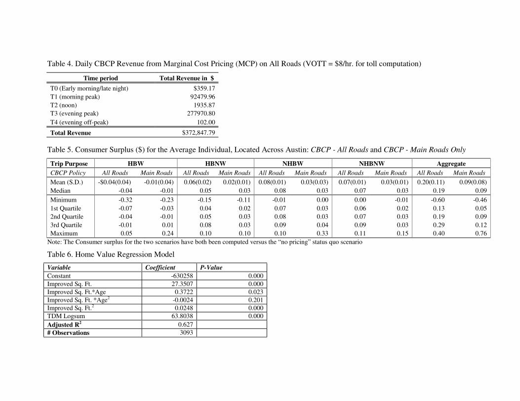
Table 4. Daily CBCP Revenue from Marginal Cost Pricing (MCP) on All Roads (VOTT = $8/hr. for toll computation)

Time period Total Revenue in $

T0 (Early morning/late night) $359.17 T1 (morning peak) 92479.96 T2 (noon) 1935.87 T3 (evening peak) 277970.80 T4 (evening off-peak) 102.00

Total Revenue $372,847.79 Table 5. Consumer Surplus ($) for the Average Individual, Located Across Austin: CBCP - All Roads and CBCP - Main Roads Only

Trip Purpose HBW HBNW NHBW NHBNW Aggregate CBCP Policy All Roads Main Roads All Roads Main Roads All Roads Main Roads All Roads Main Roads All Roads Main Roads

Mean (S.D.) -$0.04(0.04) -0.01(0.04) 0.06(0.02) 0.02(0.01) 0.08(0.01) 0.03(0.03) 0.07(0.01) 0.03(0.01) 0.20(0.11) 0.09(0.08) Median -0.04 -0.01 0.05 0.03 0.08 0.03 0.07 0.03 0.19 0.09 Minimum -0.32 -0.23 -0.15 -0.11 -0.01 0.00 0.00 -0.01 -0.60 -0.46 1st Quartile -0.07 -0.03 0.04 0.02 0.07 0.03 0.06 0.02 0.13 0.05 2nd Quartile -0.04 -0.01 0.05 0.03 0.08 0.03 0.07 0.03 0.19 0.09 3rd Quartile -0.01 0.01 0.08 0.03 0.09 0.04 0.09 0.03 0.29 0.12 Maximum 0.05 0.24 0.10 0.10 0.10 0.33 0.11 0.15 0.40 0.76

Note: The Consumer surplus for the two scenarios have both been computed versus the “no pricing” status quo scenario

Table 6. Home Value Regression Model

Variable Coefficient P-Value Constant -630258 0.000 Improved Sq. Ft. 27.3507 0.000 Improved Sq. Ft.*Age 0.3722 0.023 Improved Sq. Ft. *Age2 -0.0024 0.201 Improved Sq. Ft.2 0.0248 0.000 TDM Logsum 63.8038 0.000 Adjusted R2 0.627 # Observations 3093

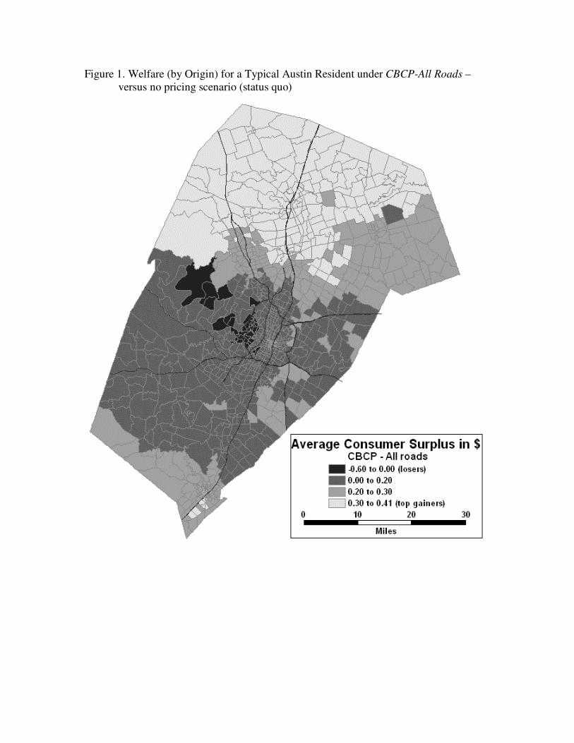
Figure 1. Welfare (by Origin) for a Typical Austin Resident under CBCP-All Roads – versus no pricing scenario (status quo)

Figure 2. Welfare (by Origin) for a Typical Austin Resident under CBCP-Main Roads – versus no pricing scenario (status quo)

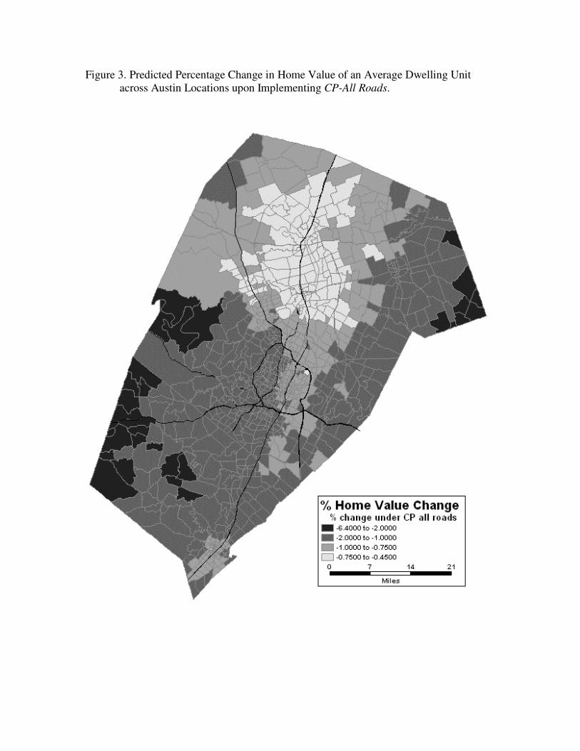
Figure 3. Predicted Percentage Change in Home Value of an Average Dwelling Unit across Austin Locations upon Implementing CP-All Roads.

Figure 4. Predicted Percentage Change in Home Value of an Average Dwelling Unit across Austin Locations upon Implementing CP-Main Roads.