CPSC 531: Probability Review1 CPSC 531:Probability & Statistics: Review II Instructor: Anirban...

CPSC 531: Probability Review 1

CPSC 531:Probability & Statistics: Review II

Instructor: Anirban MahantiOffice: ICT 745Email: [email protected] Location: TRB 101Lectures: TR 15:30 – 16:45 hoursClass web page:

http://pages.cpsc.ucalgary.ca/~mahanti/teaching/F05/CPSC531

Notes derived from “Probability and Statistics” by M. DeGroot and M. Schervish, Third edition, Addison Wesley, 2002, and

“Discrete-event System Simulation” by Banks, Carson, Nelson, and Nicol, Prentice Hall, 2005.

http://pages.cpsc.ucalgary.ca/~mahanti/teaching/F05/CPSC531


Objective and Outline The world the model-builder sees is probabilistic

rather than deterministic. Some statistical model might well describe the

variations.

An appropriate model can be developed by sampling the phenomenon of interest: Select a known distribution through educated guesses Make estimate of the parameters Test for goodness of fit

Goal is to review: Random variables Discrete and continuous random variables Cumulative distribution functions Expectation, variance, etc.


Random Variables A random variable is a real-valued mapping

defined on a sample space.

Suppose that X is a random variable defined on space S, then X assigns a real-number X(s) to each possible outcome s є S.

Typically, X, Y, Z etc denote random variables; x, y, z, etc denote values attained by random variables.

Example: Rolling a pair of dice. Let X be the random variable corresponding to the sum of the dice on a roll. If we think of the sample points as a pair (i, j), where i = value rolled by the first dice and j = value rolled by the second dice, we have:

X(s) = i+j


Discrete Random Variables A random variable X is said to be discrete if the

number of possible values of X is finite, or at most, an infinite sequence of different values.

Example: Consider jobs arriving at a job shop.• Let X be the number of jobs arriving each week at a job

shop.• S = possible values of X (range space of X) = {0,1,2,…} • p(xi) = probability the random variable is xi = P(X = xi)

p(xi), i = 1,2, … must satisfy:

The collection of pairs [xi, p(xi)], i = 1,2,…, is called the probability distribution of X, and p(xi) is called the probability mass function (pmf) of X.

The pmf is referred to as “probability function” in some texts

1 1)( 2.

i allfor ,0)( 1.

i i

i

xp

xp


Discrete Random Variables Consider a random variable X that takes on values

1, 2, 3, and 4 with probabilities 1/6, 1/3, 1/3, and 1/6, resp.

1 2

p(x)

3 4

0.35

0.30

0.25

0.20

0.15

0.10

0.05

0.00 x


Continuous Random Variables X is a continuous random variable if there exists a non-

negative function f(x) such that for any set of real numbers A є S

The probability that X lies in the interval [a,b] is given by:

f(x), denoted as the pdf of X, satisfies:

Properties

Sxxf

dxxf

Sxxf

S

in not is if ,0)( 3.

1)( 2.

in allfor , 0)( 1.

b

adxxfbXaP )()(

)()()()( .2

0)( because ,0)( 1.0

00

bXaPbXaPbXaPbXaP

dxxfxXPx

x

A

dxxfAXP )()(


Continuous Random Variables

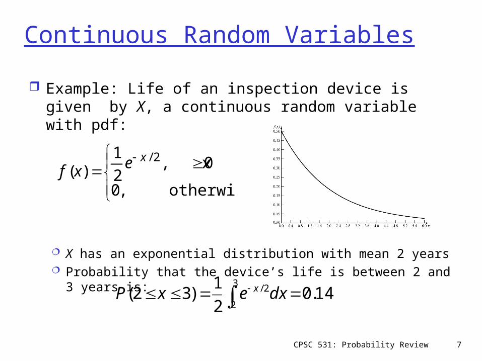
Example: Life of an inspection device is given by X, a continuous random variable with pdf:

X has an exponential distribution with mean 2 years Probability that the device’s life is between 2 and 3 years

is:

otherwise ,0

0 x,2

1)(

2/xexf

14.02

1)32(

3

2

2/ dxexP x


Cumulative Distribution Function The cumulative distribution function (cdf) of a random

variable X is a function F(x), defined for each real number x: F(x) = P(X <= x) for -∞ < x < ∞

If X is discrete, then

If X is continuous, then Properties

All probability question about X can be answered in terms of the cdf, e.g.:

xx

i

i

xpxF all

)()(

xdttfxF )()(

0)(lim 3.

1)(lim 2.

)()( then , If function. ingnondecreas is 1.

xF

xF

bFaFbaF

x

x

baaFbFbXaP allfor ,)()()(


Cumulative Distribution Function Example: An inspection device has cdf:

The probability that the device lasts for less than 2 years:

The probability that it lasts between 2 and 3 years:

2/

0

2/ 12

1)( xx t edtexF

632.01)2()0()2()20( 1 eFFFXP

145.0)1()1()2()3()32( 1)2/3( eeFFXP


Expectation The expected value of X is denoted by E(X)

If X is discrete

If X is continuous

The mean, μ, is the 1st moment of X A measure of the central tendency

Properties: E(cX) = cE(X), where c is a constant E(Y) = aE(X) + b, where Y=aX+b, a & b are constants E(X + Y) = E(X) + E(Y) regardless of whether X and Y are

independent E(X.Y) = E(X).E(Y) if X & Y are independent

xxxpXE

All)()(

dxxxfXE

)()(


Variance The variance of X is denoted by V(X) or

var(X) or 2

Definition: V(X) = E[(X – E[X]2] Also, V(X) = E(X2) – [E(x)]2

The variance is a measure of the dispersion or spread of a random variable about its mean

The standard deviation of X is denoted by Definition: square root of V(X) Expressed in the same units as the mean

Properties: V(cX) = c2V(X) V(X + Y) = V(X) + V(Y) if X, Y are independent


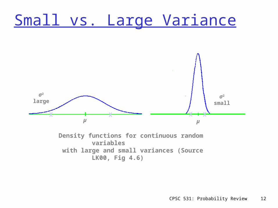
Density functions for continuous random variables with large and small variances (Source LK00, Fig 4.6)

µ µ

σ2

largeσ2

small

X X X X

Small vs. Large Variance


Expectations and Variance (example) Example: The mean of life of the previous inspection

device is:

To compute variance of X, we first compute E(X2):

Hence, the variance and standard deviation of the device’s life are:

22/2

1)(

0

2/

00

2/

dxexdxxeXE xx xe

82/22

1)(

0

2/

00

2/22

dxexdxexXE xx ex

2)(

428)( 2

XV

XV


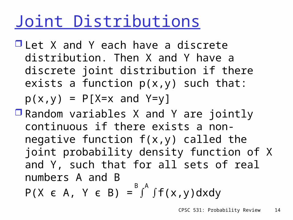
Joint Distributions Let X and Y each have a discrete

distribution. Then X and Y have a discrete joint distribution if there exists a function p(x,y) such that:

p(x,y) = P[X=x and Y=y] Random variables X and Y are jointly

continuous if there exists a non-negative function f(x,y) called the joint probability density function of X and Y, such that for all sets of real numbers A and B

P(X є A, Y є B) = ∫ ∫f(x,y)dxdyB A


Covariance

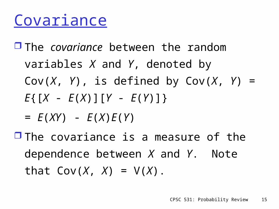
The covariance between the random

variables X and Y, denoted by Cov(X, Y), is

defined by Cov(X, Y) = E{[X - E(X)][Y -

E(Y)]}

= E(XY) - E(X)E(Y)

The covariance is a measure of the

dependence between X and Y. Note that

Cov(X, X) = V(X).


Covariance

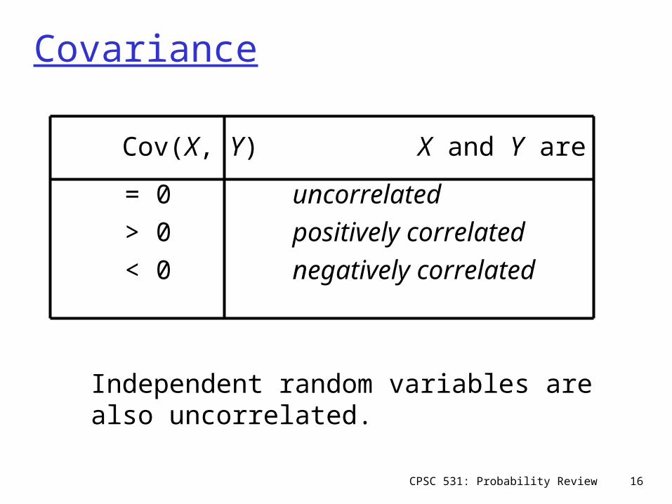
Cov(X, Y) X and Y are

= 0 uncorrelated> 0 positively correlated< 0 negatively correlated

Independent random variables are also uncorrelated.


Statistical Models Application areas where statistical models

find widespread use: Queueing systems Inventory and supply-chain systems Reliability and maintainability Limited data


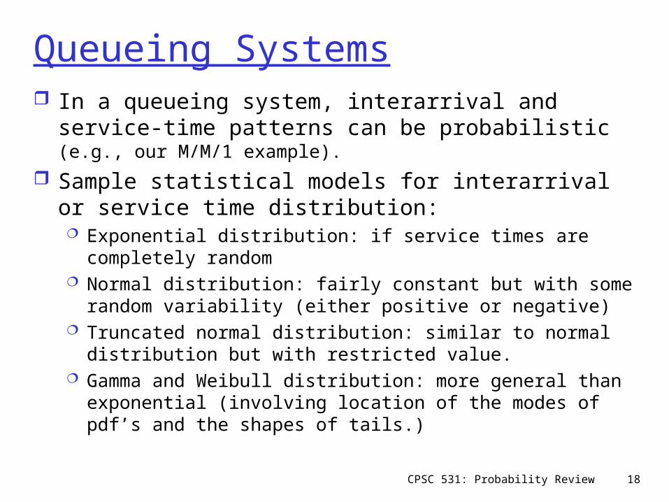
Queueing Systems In a queueing system, interarrival and service-time

patterns can be probabilistic (e.g., our M/M/1 example).

Sample statistical models for interarrival or service time distribution: Exponential distribution: if service times are completely

random Normal distribution: fairly constant but with some random

variability (either positive or negative) Truncated normal distribution: similar to normal

distribution but with restricted value. Gamma and Weibull distribution: more general than

exponential (involving location of the modes of pdf’s and the shapes of tails.)


Inventory and supply chain In realistic inventory and supply-chain systems,

there are at least three random variables: The number of units demanded per order or per time

period The time between demands The lead time

Sample statistical models for lead time distribution: Gamma

Sample statistical models for demand distribution: Poisson: simple and extensively tabulated. Negative binomial distribution: longer tail than Poisson

(more large demands). Geometric: special case of negative binomial given at

least one demand has occurred.


Reliability and maintainability Time to failure (TTF)

Exponential: failures are random Gamma: for standby redundancy where each

component has an exponential TTF Weibull: failure is due to the most serious of a

large number of defects in a system of components

Normal: failures are due to wear


Our next stop Discrete distributions, such as:

Bernoulli trials and Bernoulli distribution Binomial distribution Geometric and negative binomial distribution Poisson distribution

Continuous distributions, such as: Uniform Exponential Normal Weibull Lognormal

CPSC 531: Probability Review1 CPSC 531:Probability & Statistics: Review II Instructor: Anirban...

Documents

Transcript of CPSC 531: Probability Review1 CPSC 531:Probability & Statistics: Review II Instructor: Anirban...