hep-

ph/9

7022

64

5 Fe

b 19

97FERMILAB-CONF-96/429-T

NSF-PT-96-2November 1996

CP VIOLATION IN THE K AND B SYSTEMS†

Boris Kayser

Fermi National Accelerator Laboratory

Batavia, IL 60510 USA

and

National Science Foundation*

4201 Wilson Boulevard

Arlington, VA 22230 USA

Abstract

Although CP violation was discovered more than thirty years

ago, its origin is still unknown. In these lectures, we describe the CP-

violating effects which have been seen in K decays, and explain how

CP violation can be caused by the Standard Model weak interaction.

The hypothesis that this interaction is indeed the origin of CP viola-

tion will be incisively tested by future experiments on B and K decays.

We explain what quantities these experiments will try to determine,

and how they will be able to determine them in a theoretically clean

way. To clarify the physics of the K system, we give a phase-conven-

tion-free description of CP violation in this system. We conclude by

briefly exploring whether electric dipole moments actually violate CP

even if CPT invariance is not assumed.

† To appear in the Proceedings of the Summer School in High Energy Physics and Cosmology, held

at the International Center for Theoretical Physics, Trieste, June-July 1995.

* Permanent Address

1

1. Preamble

Being lovers of symmetry, we are tempted to expect that the behavior of a

physical system will not change at all if we replace every particle in it by its anti-

particle. However, in some processes nature violates this expected matter-anti-

matter symmetry. Particularly interesting is the violation of invariance under

CP, the combined action of charge conjugation C and parity P. Before we turn to

CP, let us first briefly consider the simplest operation which replaces a particle by

its antiparticle, namely C.

The effect of C on a particle f(→p ,λ) of momentum

→p and helicity λ is given by

Cf(→p ,λ)⟩ = ηC

–f (

→p ,λ)⟩ , (1.1)

where –f is the antiparticle of f, and ηC is a phase factor. Note that C does not alter

a particle’s momentum or helicity.

It has long been known that some processes are not invariant under C.

Consider, for example, the decay π → µν. Invariance under C would require that

the muons produced in π+ → µ+ + ν and π− → µ− +ν have identical helicity. But it

is found that actually they have opposite helicity: the µ+ in π+ decay is always left-

handed, while the µ− in π− decay is always right-handed. Thus, π → µν is not

invariant under C.

A somewhat more subtle operation which replaces a particle by its antipar-

ticle is CP. The effect of CP on f(→p ,λ) is given by

CPf(→p ,λ)⟩ = ηCP

–f (–

→p ,–λ)⟩ , (1.2)

Here, the momentum and helicity reversals are due to the action of P, and ηCP is a

phase factor.

From Eq. (1.2), the CP-mirror image of the decay π+ → µLH+  + ν, where the

subscript LH reminds us that the µ+ has left-handed helicity, is the decay π− →µRH

–   + ν, in which the µ– has right-handed helicity. These two decays are the ones

actually observed, and they have equal rates. Thus, π→ µν, while not invariant

under C, is invariant under CP.

One might wonder whether perhaps all processes, even those which are not

invariant under C, are nevertheless invariant under CP. The decays of the neu-

tral K mesons have taught us that this is not the case. Let us turn, then, to the

phenomenology of the neutral kaon system.

2

2. CP Violation in the Neutral K System

Let us consider neutral kaons at rest. We choose our phase conventions in

this Section so that

CPK0⟩ = +—K0⟩ . (2.1)

Simple field theory then implies that

CP—K0⟩ = +K0⟩ . (2.2)

In Section 5, we shall free ourselves of this phase convention, and adopt a conven-

tion-free formalism.

While K0 and —K0 have opposite strangeness, the weak interactions do not

conserve strangeness, and so they mix K0 and —K0. The time evolution of a neutral

kaon is then described by a two-component Schrödinger equation of the form

i

∂∂t

a(t)

a(t)

= M

a(t)

a(t)

. (2.3)

Here, a(t) is the amplitude for us to have a K0 at time t, anda(t) is the amplitude

for us to have a —K0. The quantity M is a 2x2 matrix,

M =K0|M|K0 K0|M|K0

K0|M|K0 K0|M|K0

≡M 11 M 12

M 21 M 22

, (2.4)

known as the neutral K mass matrix, which serves as the effective Hamiltonian

for a neutral kaon at rest. Since a kaon disappears with time through its decay, M

is non-Hermitean.

We shall assume that the world is CPT invariant. It is readily shown that

this invariance implies that

M11 ≡ ⟨K0MK0⟩ = ⟨—K0M

—K0⟩ ≡ M22 . (2.5)

Writing M11 ≡ M – iΓ/2, and M22 ≡ —M – i

–Γ/2, we see that the real part of Eq. (2.5), M

= —M , is an example of the well-known CPT requirement that a particle and its anti-

particle have the same mass. The imaginary part, Γ = –Γ, is an example of the re-

quirement that they have the same total width or, equivalently, the same lifetime.

3

Assume for the moment that CP invariance holds. Then our effective

Hamiltonian obeys (CP)†M (CP) = M, and we have

M12 ≡ ⟨K0M—K0⟩ = ⟨K0(CP)†M (CP)

—K0⟩

= ⟨(CP)K0M(CP)—K0⟩ = ⟨

—K0MK0⟩ ≡ M21 . (2.6)

Thus, from Eqs. (2.5) and (2.6), M has the form

M =

X Y

Y X

. (2.7)

The eigenstates of M—the mass eigenstates of the neutral K system—are then

1

2

1

1

and

1

2

1

−1

. That is, they are the CP eigenstates

K1 = 1

2K0 + K0

(2.8)

and

K2 = 1

2K0 − K0

. (2.9)

Note that K1⟩ and K2⟩ have opposite CP parity:

CPK1(2)⟩ = +(–)K1(2)⟩ . (2.10)

Now, experimentally, the two mass eigenstates of the neutral K system are

the K-short KS, with a short lifetime τS = (0.8926 ± 0.0012) x 10–10 sec, and the K-

long KL, with a much longer lifetime τL = (5.17 ± 0.04) x 10–8 sec. Essentially all KS

decays are to π+π– or π0π0. It is easy to show that both of these final states have CP

= +1. Thus, if CP invariance and the associated CP conservation law hold, KS

must be K1. Then KL must be K2. But then, since K2 has CP = –1, the decays KL →π+π– and KL → π0π0 are forbidden. Nevertheless, these decays do occur.1 Thus, CP

is violated in neutral K decays.

To be sure, the observed violation is small. The amplitudes for the CP-violat-

ing decay KL → π+π– and the CP-conserving one KS → π+π– are in the ratio2

π +π − T KL

π +π − T KS

= (2.285 ± 0.019) × 10−3 . (2.11)

4

Similarly,2

π0π0 T KL

π0π0 T KS

= (2.275 ± 0.019) × 10−3 . (2.12)

Nevertheless, this violation of CP is nonvanishing. Like C, CP is a symmetry

which is not always respected.

In addition to KL → ππ, other CP-violating effects have been seen in the

neutral kaon system. One of these is found in the semileptonic decays KL → πlν,

where l is an e or a µ. When CP invariance holds, the KL is a CP eigenstate. Then

the CP-mirror image of the decay KL → π–l+ν is KL → π+l––ν. To be sure, CP

reverses the momenta and helicities of all the outgoing particles, but that is irrel-

evant when we integrate over these variables to get the full rate for decay into the

particles under consideration. Thus, when CP invariance holds, we require that

Γ(KL → π–l+ν ) = Γ(KL → π+l––ν). However, it is found experimentally that2

δ ≡

Γ KL → π −l

+ν( ) − Γ KL → π +l

−ν( )" + "

= 3.27 ± 0.12 x 10–3 . (2.13)

Further observed CP-violating effects will be discussed in Section 5.

3. The Origin of CP Violation in the Standard Model

All CP-violating effects observed to date have been seen in the decays of neu-

tral kaons. These decays are known to be due to the weak interaction. Therefore, it

is natural to speculate that CP violation may well be an effect of the weak inter-

action. This is the possibility that we shall emphasize here.

The weak interaction is very successfully described by the so-called

Standard Model (SM). In the SM, the weak interaction is carried by the charged

weak boson W, and the neutral weak boson Z. These bosons couple to the leptons

and to the three generations, or families, of quarks:

Generation: 1 2 3

Charge = 2/3Charge = –1/3

u

d

c

s

t

b

Mass

5

As indicated, the quarks in the third generation are the heaviest ones, those in the

second generation are lighter, and those in the first generation are lighter still. In

a typical Feynman diagram for a hadronic weak decay, a relatively heavy quark

decays to lighter ones via W exchange. This is illustrated in Fig. 1, in which a KS

decays via its —K0⟩ ( =s

–d⟩) component into π+π–. The diagram of Fig. 1 entails the

W-mediated quark decay s → u–ud.

Vus u

d

–u

–d

s

Vud*

π+

π–

Ks

W–

Figure 1. One of the diagrams for KS → π+π−.

According to the SM, the coupling of the W boson to the quarks is given by

the Hamiltonian

H W = g

2W µ Vαi αLγ µ iL

α =u,c,ti=d,s,b

∑ + g

2W µ†

Vαi* iLγ µαL

αi

∑ . (2.14)

Here, g is a real overall coupling strength, W is the W boson field, αL ≡ 1–γ5

2α is

the left-handed projection of the quark field α and similarly for iL, and the numer-

ical coefficients Vαi are the elements of the Cabibbo-Kobayashi-Maskawa (CKM)

quark mixing matrix

V =Vud Vus Vub

Vcd Vcs Vcb

Vtd Vts Vtb

. (2.15)

Note from Eq. (2.14) that any of the three negatively-charged quarks i can turn into

any of the three positively-charged ones α by emitting a W–, the amplitude for its

doing so being proportional to Vαi. Thus, the off-diagonal elements of V describe

transitions in which a quark in one family turns into a quark in another family.

Hence, these elements mix the families, earning for V the name "quark mixing

matrix".

6

The SM coupling of the Z boson to the quarks is described by the

Hamiltonian

H Z = g

cosθW

Zµ I3 qL( ) − Q q( )sin2 θW[ ]qLγ µqL − Q q( )sin2 θW qRγ µqR{ }q=u,c,t,

d,s,b

∑ . (2.16)

Here, θW is the Weinberg angle, I3(qL) is the weak isospin of the left-handed

quark qL, Q(q) is the electric charge of q, and qR ≡ (1+γ5)

2q is the right-handed

projection of the quark field q.

Under CP, the term

g

2W µVαiαLγ µ iL in the W-quark interaction HW trans-

forms as

CP( ) g

2W µVαiαLγ µ iL CP( )−1 = η* W( )η α( )η* i( )[ ] g

2W µ†

VαiiLγ µαL . (2.17)

Here, η(W), etc. are phases, and we may choose [η*(W)η(α)η*(i)] = 1. Then

H W = g

2W µ VαiαLγ µ iL

α ,i∑ + g

2W µ†

V*αiiLγ µαLα ,i∑

CP → g

2W µ†

VαiiLγ µαLα ,i∑ + g

2W µ V*αiαLγ µ iL

α ,i∑

. (2.18)

We see that HW is CP-invariant if, and only if, V is real, or can be made real by

changing the phase conventions for the quark fields.

The analogue of Eq. (2.17) for the terms in the Z-quark interaction HZ states

that each of these terms transforms back into itself under CP. Thus, HZ is neces-

sarily CP-invariant.

We conclude that in the SM weak interaction, CP violation can arise only if

some of the numbers Vαi are complex. How their complexity can produce physi-

cal CP-violating effects will be explained shortly.

3.1. The CKM Matrix

The SM requires that the CKM quark mixing matrix be unitary. Apart from

this unitarity, the matrix is not predicted, so its elements must be determined

experimentally.

7

How many independent parameters are needed to determine fully the CKM

matrix V? In answering this question, we must bear in mind that some of the

complex phases which V may contain are not physically meaningful. To see this,

note from Eq. (2.14) that, apart from irrelevant factors, Vαi is just the amplitude

⟨αHWi⟩ for the quark transition i → α through W emission. Thus, if the arbi-

trary relative phase of the i and α quarks is changed, the phase of Vαi will change

correspondingly. Redefining the down-type quark i by i⟩ → eiθi⟩ multiplies the i

column of V by eiθ. Similarly, phase redefining the up-type quark α multiplies the

α row of V by a phase factor. Hence, without changing the physics, we may mul-

tiply any column or row of V by a phase factor, or carry out any number of such

operations. We may use these operations to remove from V five phases corre-

sponding to the five relative phases of the six quarks, leaving five of the elements

of V real. We may do this, for example, by multiplying each of the columns of V by

a phase factor chosen to make its bottom element real, and then multiplying each

of the top two rows by a phase factor chosen to make its rightmost element real.

Mindful of this freedom to remove at least some phases from V, let us now

suppose that there are, not just three doublet quark families, but N of them, so

that V becomes an NxN matrix. How many parameters are necessary to deter-

mine it completely? Before constraints are imposed, 2N2 real numbers are

required to fully specify the N2 complex elements of V. But the unitarity of V

demands that the sum of the absolute squares of the elements in any of its

columns be unity—a demand that imposes N constraints. Furthermore, unitarity

demands that any two of the columns of V be orthogonal. Now, there are N(N–1)/2

pairs of columns, and the equation expressing the orthogonality of any pair has

both a real and an imaginary part. Thus, orthogonality of columns imposes N(N–

1) constraints. Hence, the most general NxN unitary matrix depends on 2N2 – N

– N(N–1) = N2 real parameters. Now, in the N quark families there are 2N

quarks, with 2N–1 relative phases. Thus, 2N–1 phases in V are not physically

meaningful, and may be removed by phase redefinitions of the quarks or, equiva-

lently, by multiplying columns and rows of V by phase factors. Hence, the number

of physically meaningful independent real parameters in V is N2 – (2N–1) = (N–1)2.

One possible choice for these parameters is mixing angles (parameters

which would be present even if V were real) and phases. To calculate the number

of mixing angles on which V depends, imagine that it is real. It is then an ortho-

gonal (i.e., a rotation) matrix. It contains N2 real elements, subject to N con-

straints expressing the requirement that each of its columns be a vector of unit

length, and N(N–1)/2 constraints expressing the requirement that any pair of its

columns be orthogonal. Thus, V depends on N2 – N – N(N–1)/2 = N(N–1)/2 mix-

ing angles.

8

In summary, the complex NxN quark mixing matrix depends on (N–1)2

parameters. If we take these to be mixing angles and phases, N(N–1)/2 of them

are mixing angles, so that (N-1)2 – N(N–1)/2 = (N–1)(N–2)/2 of them are phases.

Note from this result that there are no physically significant phases in the mixing

matrix unless N ≥ 3.3 Had there been fewer than three quark families, it would

have been impossible for the weak interaction, as described in the SM, to violate

CP.

(It is instructive and easy to explicitly construct the most general unitary

quark mixing matrix for the case N = 2, and show that all phases can be removed

from this matrix by multiplying its rows and columns by phase factors. Since this

leaves the matrix real, it cannot violate CP.)

Although there are in reality (at least) three quark families, the fact that

the quark mixing matrix cannot violate CP in a world with only two families has

an important consequence. Namely, it implies that CP violation in K decays will

be small, as observed, even if the complex phases in the true 3x3 mixing matrix

are large. Furthermore, it tells us where we must look if we wish to see large CP-

violating effects.4 To see why it implies that CP violation in K decays will be small,

note that, as illustrated in Fig. 1, the dominant diagrams for K decays involve only

quarks from the first two families. The quarks t and b are not involved. Thus, in

first approximation, K decays “do not know” that there are not just two, but three

quark generations. In this approximation, K decay processes do not contain

enough physics to violate CP. Now, when one goes beyond the first approximation,

one finds that K decays do involve the quarks of the third generation in several

ways, so that these reactions can (and do!) violate CP. However, because one must

go beyond the leading approximation before the third generation quarks come into

the picture, CP violation in K decays is small.

From this discussion, it is clear that if we wish to see large CP-violating

effects coming from the CKM matrix, we must look for them in processes which

involve, even in leading approximation, quarks from all three generations. To this

end, new facilities are being built and new experiments are being developed

which will study CP violation in the decays of the B or beauty mesons. The B

mesons and their quark content are

B+ = [b–

u] B– = [bu–

]

Bd = [b–

d]—Bd = [bd

–]

Bs = [b–

s]—Bs = [bs

–]

Bc = [b–

c]—Bc = [bc

–] .

9

In a typical B decay, the heavy b orb quark in the B—a quark of the third genera-

tion—decays down to lighter quarks in the first and/or second generations. Often,

all three generations are involved. Thus, CP violation can be large.

As we shall see shortly, the CP-violating effects in B decays can also yield

clean information on the phases in the CKM matrix. Thus, the study of these

effects will be a very good test of whether these phases are indeed the origin of CP

violation.

4. CP Violation in the B System

The effects to be sought in the B system are CP-violating inequalities

between the rates for CP-mirror-image decays. When CP invariance holds, the

amplitude ⟨fTi⟩ for the decay of any initial state i into any final one f obeys

⟨fTi⟩ = ⟨CP[f]TCP[i]⟩ . (4.1)

Thus, for example, any inequality between the rates for the CP-mirror-image

decays B+ → f and B– →f, wheref ≡ CP[f] is the CP-mirror image of the final

state f, is a violation of CP invariance. It is violations of this general sort, which

are B-system analogues of the K-system asymmetry δ of Eq. (2.13), which will be

sought.

As we noted earlier, CPT invariance, which we assume to hold exactly,

requires that any unstable particle and its antiparticle have the same total width.

Thus, if there is some final state f for which, in violation of CP, Γ[B+ → f] > Γ[B–

→f], then there must be some other final state (or states) f′ for which Γ[B+ → f′] <Γ[B– →f′]. Otherwise, the CPT constraint that Γtotal [B+] = Γtotal[B–] could not be

satisfied.

The complex phases in the CKM matrix, like complex phases anywhere in

quantum mechanics, lead to physical consequences only through interferences

between amplitudes. In particular, it is through interferences that the CKM

phases produce CP violation. How they do this is nicely illustrated by the compari-

son between the CP-mirror-image processes B+ → f and B– →f. Suppose that the

weak decay B+ → f receives contributions from two Feynman diagrams. Each of

these diagrams is proportional, like the diagram of Fig. 1, to some product of

CKM elements. Thus, the amplitude a for the first diagram has the form

a = MeiδCKMf

eiαS , (4.2)

10

where M is the magnitude of a, δ f  CKM is the phase of the product of CKM elements

to which the diagram is proportional, and αS is a phase arising from strong in-

teraction effects such as final-state rescattering. Similarly, the amplitude a′ for

the second diagram has the form

′a = ′M ei ′δCKMf

ei ′αS , (4.3)

where M' ≡ a′, δ ′ f  CKM is the phase of the product of CKM elements to which the

second diagram is proportional, and α ′S is the strong-interaction phase of this

diagram. The rate for B+ → f is then

Γ B+ → f[ ] = MeiδCKMf

eiαS + ′M ei ′δCKMf

ei ′αS

2

= M2 + ′M 2 + 2M ′M cos ϕ + ϕS( ) , (4.4)

where ϕ ≡ δ f  CKM – δ ′ f  CKM is the relative CKM phase of the two amplitudes, and ϕS ≡

αS – α′S is their relative strong-interaction phase.

Now, the diagrams for the CP-mirror-image decay B– →f are, of course,

the same as those for B+ → f, except that every quark (antiquark) is replaced by its

antiquark (quark). From HW, Eq. (2.14), we see that, owing to this replacement,

every CKM element appearing in a diagram for B+ → f is replaced by its complex

conjugate in the corresponding diagram for B– →f. However, apart from CKM

phases, the SM weak interaction of Eqs. (2.14) and (2.16) is completely CP invari-

ant, as is the SM strong interaction. Thus, apart from the reversal of its CKM

phase, the amplitude of a diagram does not change at all when we go from B+ → fto B– →f. Hence, the rate for B– →f is

Γ B− → f[ ] = Me−iδCKMf

eiαS + ′M e−i ′δCKMf

ei ′αS

2

= M2 + ′M 2 + 2M ′M cos −ϕ + ϕS( ) . (4.5)

Comparing Eqs. (4.4) and (4.5), we see that when CKM phases are present,

the two interfering amplitudes can have a different relative phase in B– →f than

they do in B+ → f. As a result, Γ[B– →f] and Γ[B+ → f] can differ, in violation of

CP.

To test the SM of CP violation, one would like not only to observe a CP-violat-

ing inequality between Γ[B+ → f] and Γ[B– →f], but also to determine the CKM

phase ϕ. Of course, Γ[B+ → f] and Γ[B– →f] are only two measurable quantities,

and as we see from Eqs. (4.4) and (4.5), they depend on four parameters: M, M′, ϕ,

11

and ϕS. Thus, by themselves, they cannot determine ϕ. Consequently, in general,

a clean test of the SM of CP violation is not possible in decays of charged B mesons.

(To be sure, in the exceptional cases where M and M′ can be determined indepen-

dently of Γ[B+ → f] and Γ[B– →f], the measurement of these two decay rates de-

termines sin2ϕ, up to a two-fold ambiguity, and so does provide a test of the SM.5)

4.1. Decays of Neutral B Mesons

In decays of neutral B mesons, a clean test of the SM of CP violation is

possible. To see why, let us discuss the Bd – —Bd system; the Bs –

—Bs system behaves

similarly.

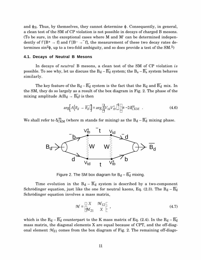
The key feature of the Bd – —Bd system is the fact that the Bd and

—Bd mix. In

the SM, they do so largely as a result of the box diagram in Fig. 2. The phase of the

mixing amplitude A(Bd → —Bd) is then

arg A Bd → Bd( )[ ] = arg VtdVtb

*( )2

≡ −2δCKMm . (4.6)

We shall refer to δ m  CKM (where m stands for mixing) as the Bd –

—Bd mixing phase.

Vtb*

Bd Bd

b

b

t

td

d

W W

Vtd

Vtb*Vtd

Figure 2. The SM box diagram for Bd – —Bd mixing.

Time evolution in the Bd – —Bd system is described by a two-component

Schrödinger equation, just like the one for neutral kaons, Eq. (2.3). The Bd – —Bd

Schrödinger equation involves a mass matrix,

M =

X M 12

M 21 X

, (4.7)

which is the Bd – —Bd counterpart to the K mass matrix of Eq. (2.4). In the Bd –

—Bd

mass matrix, the diagonal elements X are equal because of CPT, and the off-diag-

onal element M21 comes from the box diagram of Fig. 2. The remaining off-diago-

12

nal element, M 12, comes from a similar box diagram in which every quark

(antiquark) has been replaced by its antiquark (quark). As in the case of charged B

decays, this means that every CKM element has been replaced by its complex con-

jugate, but there have been no other changes. Since the box diagram of Fig. 2 has

no strong phase (owing to the fact that the B meson is far belowtt threshold), we

see that

M12 = M21(V → V*) = M *21 . (4.8)

Let us call the mass eigenstates of the Bd – —Bd system BHeavy (BH) and

BLight (BL). From Eq. 4.7, the complex masses of these mass eigenstates—the

eigenvalues of M— are

λH(L) = X +

(−) M 12M 21 ≡ mH(L) − i

2ΓH(L) . (4.9)

Here, mH(L) are the masses of BH(L), respectively, and ΓH(L) are their widths.

Note that since M12M21 is real and positive, so that λH and λL have the same

imaginary part, the widths of BH and BL are equal:

ΓH = ΓL ≡ Γ . (4.10)

(To a very good approximation, this equality holds even if the SM diagram of Fig. 2

is not a good approximation to A(Bd → —Bd). This is simply because, unlike KS and

KL, neither B mass eigenstate has a special decay mode which is an appreciable

fraction of its decays and which is unavailable to the other mass eigenstate. Thus,

BH and BL have approximately equal widths.)

From Eqs. (4.7) and (4.9), the mass eigenstates BH(L)⟩ are given by

BH(L) = 1

2Bd

+(−) e

−2iδCKMm

Bd

. (4.11)

Here and hereafter we assume that M21 does come from the SM diagram of Fig. 2.

Owing to the Bd ——Bd mixing, a neutral B at rest which at time t = 0 is a

pure Bd⟩ will not remain that way. Rather, in time t it will evolve into a state

Bd(t)⟩ which is a coherent superposition of Bd⟩ and —Bd⟩. From Eqs. (4.9), (4.11),

and Schrödinger’s equation, it is straightforward to show that

Bd(t) = e

−i m−iΓ2

t

c Bd − ie−2iδCKMm

s Bd{ } . (4.12)

13

Here,

m ≡ mH + mL

2(4.13)

is the average BH, BL mass,

∆m ≡ mH – mL (4.14)

is the BH – BL mass difference, and

c ≡ cos (∆m

2t), s ≡ sin (

∆m

2t) . (4.15)

Note from Eq. (4.12) that, before it decays into some final state, a neutral B meson

which at time t = 0 is a pureBd⟩ oscillates between being a Bd⟩ and a —Bd⟩. This

oscillation has been observed,6 and it is found that

∆m

Γ= 0.66 ± 0.09 ARGUS & CLEO7

0.72 ± 0.04 LEP6,8

Thus, before a typical B decays, it undergoes a non-negligible fraction of one oscil-

lation.

Suppose, now, that f is a final state into which both a pure Bd and a pure —Bd

can decay. Examples of such a final state are ρ+π–, D

0Ks, π

+π–, and ΨKs. Let Γf(t) ≡

Γ(Bd(t) → f) be the time-dependent probability for the time-evolved particle Bd(t),

which at t = 0 was a pure Bd, to decay into f. From the wave function for Bd(t), Eq.

(4.12), Γf(t) is given by

Γ f (t) = f T Bd(t)

2= e−Γt c f T Bd − ie−2iδCKM

m

s f T Bd

2 . (4.16)

Let us now assume that the decay amplitudes ⟨fTBd⟩ and ⟨fT—Bd⟩ are each

dominated by a single Feynman diagram. Then

f T Bd = MeiδCKMf

eiαS , (4.17)

where M is the magnitude of the diagram which dominates ⟨fTBd⟩, δ f  CKM is the

phase of the product of CKM elements to which this diagram is proportional, and

αS is the strong interaction phase of the diagram. Similarly,

f T Bd = Me−iδCKM

f

eiαS , (4.18)

14

where —M , –

–δ f

  CKM, andαS are respectively the magnitude, CKM phase, and strong

phase of the diagram which dominates ⟨fT—Bd⟩. From Eqs. (4.16)-(4.18), we then

have9

Γf(t) = e–Γt

{c2M

2 + s

2—M

2 – 2csM

—M sin (ϕ + ϕs)} , (4.19)

where

ϕ ≡ 2δCKMm + δCKM

f + δCKMf

(4.20)

is the relative CKM phase of the two interfering amplitudes in Eq. (4.16), and

ϕS = αS –αS (4.21)

is their relative strong phase.

The CP-mirror image of the decay Bd(t) → f is the process —Bd(t) →f, where

—Bd(t) is the time-evolved particle which at time t = 0 is a pure

—Bd. As before, when

we go from a process to its CP-mirror image, the CKM phases reverse, but noth-

ing else changes. Thus, from the expression (4.19) for Γf(t), we may infer that the

probability –Γ f

–(t) ≡ Γ(—Bd(t) →f) is given by9

–Γ f–(t) = e

–Γt {c2

M2 + s

2—M

2 – 2csM

—M sin (–ϕ + ϕs)} . (4.22)

Now, since Bd(t) → f and —Bd(t) →f are CP-conjugate reactions, CP invari-

ance would require that Γf(t) = –Γ f

–(t). Comparing Eqs. (4.19) and (4.22), we see that

when ϕ ≠ 0, this requirement is violated. Note that, as always, the CKM phase ϕproduces this CP violation through an interference; in this case the interference

between the two terms in Eq. (4.16), or between their analogues in —Bd(t) →f.

Physically, the first term in Eq. (4.16) corresponds to a Bd remaining a Bd and

decaying directly into f. The second term corresponds to a Bd evolving, through

mixing, into a —Bd, which then decays into f.

Recalling that Γ and ∆m are already known, it is trivial to see from Eqs.

(4.19) and (4.22) that measurements of the functions Γf(t) and –Γ f

–(t) will determine

M, —M , s+ ≡ sin (ϕ + ϕs) and s– ≡ sin (–ϕ + ϕs). Once s+ and s– are known, one can

find sin2ϕ, up to a two-fold ambiguity, by using

sin2 ϕ = 1

21 − s+s− ± (1 − s+

2 )(1 − s−2 )

. (4.23)

15

Note that, apart from the discrete ambiguity, this expression gives a theoretically

clean value for sin2ϕ. This value does not depend on any unknown or difficult-to-

calculate parameters. This value can be compared directly to the prediction from

the CKM matrix to test cleanly whether phases in this matrix are indeed the

source of CP violation.

As we have seen, the CKM phase ϕ which is probed in a given decay, Bd(t) →f, is the relative CKM phase of the two interfering terms in Eq. (4.16). That is,

recalling Eq. (4.6),

ϕ = →→ →

CKM Phase

A B f

A B B A B fd

d d d

( )

( ) ( ) , (4.24)

where “A” denotes an amplitude. As an example, in Bd(t) → ρ+π–, we expect A(Bd

→ ρ+π–) to be dominated by the diagram in Fig. 3. Similarly, we expect

—Bd → ρ+π–

to

be dominated by the diagram in Fig. 4.

Vub u–d–

u

–b

d

Vud

*

ρ+

π–Bd

Figure 3. The diagram which dominates Bd → ρ+π–.

Vub u

d

–u

–d

b

Vud*

ρ+

π–

Bd—

Figure 4. The diagram which dominates —Bd → ρ+π–.

The mixing amplitude A(Bd → —Bd) is dominated by the diagram in Fig. 2. Thus, in

Bd(t) → ρ+π–,

16

ϕ =( )

= [ ]

arg

arg

*

* *

* *

V V

V V V V

V V V V

ud ub

td tb ub ud

ud ub tb td

2

2

. (4.25)

In a similar way, one may easily find what CKM phase ϕ is probed by any particu-

lar decay. Note that since each of the amplitudes in Eq. (4.24) is always propor-

tional to some product of CKM elements (assuming each amplitude is dominated

by one diagram), ϕ is always the phase of some product and quotient, or equiva-

lently of some product, of CKM elements.

The neutral B decay rates, and the extraction of a CKM phase from them,

become particularly simple when the final state f is a CP eigenstate. Examples of

such a final state are π+π– and (neglecting CP violation in the kaon system) ΨKs.

When f is a CP eigenstate, we have f–⟩ ≡ CPf⟩ = ηff⟩, where ηf is the CP parity of

f⟩. Then ⟨fT—Bd⟩ = ηf⟨f

–T—Bd⟩. Now,

—Bd is the CP conjugate of Bd, andf is the

CP conjugate of f, so ⟨f–T—

Bd ⟩ is the CP conjugate of ⟨fTBd⟩. As before, CP-con-

jugate amplitudes have opposite CKM phase but are otherwise identical. Thus,

from Eq. (4.17), when f is a CP eigenstate,

f T Bd = η f Me−iδCKM

f

eiαS . (4.26)

Using this relation and Eq. (4.17) in Eq. (4.16), we find that

Γf(t) = M2e

–Γt{1 – ηf sinϕ sin(∆m t)} , (4.27)

where ϕ, the relative CKM phase of the two interfering terms, is now given by

ϕ = 2 δCKM

m + δCKMf( ) . (4.28)

For the CP-mirror-image decay, —Bd(t) → f, the decay rate

–Γf(t) must be the same as

Γf(t) except for a reversal of the CKM phase. That is,

–Γf(t) = M2e

–Γt{1 + ηf sinϕ sin(∆m t)} . (4.29)

Now, ∆m is known, as is the CP parity ηf of any particular final state f of interest.

Thus, the CP-violating asymmetry between –Γf(t) and Γf(t),

Γ f (t) − Γ f (t)

" + "= η f sinϕ sin ∆mt( ) , (4.30)

17

cleanly determines the CKM phase quantity sinϕ.10

It should be emphasized that the ability to cleanly extract CKM phase

information from decay rates does depend on the assumption that ⟨fTBd⟩ and

⟨fT—Bd⟩ are each dominated by one Feynman diagram. When ⟨fTBd⟩ or ⟨fT—

Bd⟩involves several competing diagrams with different CKM phases, the rate for Bd(t)

→ f involves several interferences, rather than just one, and no longer cleanly

determines any one relative CKM phase of two amplitudes. Fortunately, in at

least some of the decay modes of greatest interest, there are strong reasons for

believing that one diagram does dominate.11

4.2. Future Experiments

In Section 3, it was argued that CP-violating effects in B decay can be large.

We now see, for example, from Eq. (4.30) for the asymmetry in decay to a CP

eigenstate, that these effects can indeed be large. If the CKM phase quantity sinϕin the asymmetry (4.30) is O (1), then obviously the asymmetry itself is O (1).

However, it will take a large sample of B mesons to observe even a large CP-violat-

ing asymmetry. The reason is that each of the asymmetries on which the experi-

mental search will focus occurs in the decay to some specific final state, or CP-

conjugate pair of final states, and the branching ratio for B decay to any of the

final states of interest is rather small. Thus, a lot of B mesons will be required

before a CP-asymmetry in some particular decay mode can be seen.

As an example, consider the CP eigenstate final state f = ΨKs. If the decay

rate Γ[Bd(t) → ΨKs] is measured by observing N events, the measurement has a

statistical error of order √N. Similarly for Γ[—Bd(t) → ΨKs]. Thus, if the asymmetry

Γ Bd(t) → ΨKs[ ] − Γ Bd(t) → ΨKs[ ]" + "

(4.31)

is, for example, of order 0.1, we must have √N << (0.1)N in order to measure it with

any accuracy. Hence, we require N >~ 10

3. Now, typically a Ψ is detected via its

decay to µ+µ– or e

+e

–. Since only 12% of Ψ particles decay in this way, we need ~10

4

Bd(t) → ΨKs events in order to detect 103 of them. Furthermore, BR(Bd(t) → ΨKs) ≅

4x10–4

.2 Thus, to detect 103 Bd→ΨKs decays, we need ~10

8 Bd mesons. For other

typical decay modes of interest, the number of Bd mesons required is similar.

However, the total number of Bd mesons recorded to date at CESR, for example, is

only ~5x106.12 To produce and study enough B mesons to measure CP-violating

asymmetries in the B system, future experiments are being planned for hadron

facilities, and special high-luminosity e+e

– colliders (“B factories”) are being built

18

at SLAC and KEK. The experiments to be done at the hadron facilities and the B

factories will complement each other nicely.

To experimentally compare the rate for Bd(t) → f with that for —Bd(t) →f (or,

when f is a CP eigenstate, that for —Bd(t) → f), we must, of course, be able to distin-

guish a Bd(t) from a —Bd(t). That is, we must be able to tag the B as having been a

pure Bd, or a pure —Bd, at some specific time t = 0. Several methods for doing this

are being considered. Let us briefly review them.

At the B factories, B mesons will be produced in pairs via the reaction

e+e

– → Υ(4s) → Bd

—Bd . (4.32)

Since the Υ(4s) [the upsilon(4s)] has intrinsic spin S = 1, and B mesons are spin-

less, the B pair created in this reaction will be in a p wave. Now, after it is pro-

duced, each B meson in the pair will evolve, thanks to mixing, into a coherent

mixture of pure Bd and pure —Bd. However, at no time can one have two identical

bosons in an antisymmetric state such as a p wave. Thus, if at some time which

we shall call t = 0, one of the B mesons in the pair decays in a fashion which re-

veals that at the instant of decay it is, say, a —Bd, then, at the same instant, the

other B meson in the pair must be a Bd. That is, the decay of the one B at t = 0 tags

the remaining B as a Bd(t). This type of tagging is an interesting modern applica-

tion of the quantum mechanical correlation first discussed by Einstein, Podolsky,

and Rosen (the EPR effect).

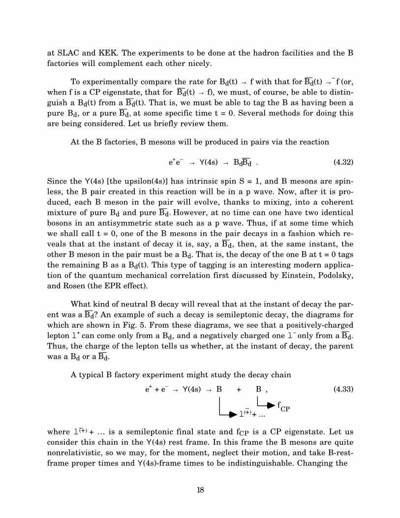
What kind of neutral B decay will reveal that at the instant of decay the par-

ent was a —Bd? An example of such a decay is semileptonic decay, the diagrams for

which are shown in Fig. 5. From these diagrams, we see that a positively-charged

lepton l+ can come only from a Bd, and a negatively charged one l

– only from a

—Bd.

Thus, the charge of the lepton tells us whether, at the instant of decay, the parent

was a Bd or a —Bd.

A typical B factory experiment might study the decay chain

e+ + e

– → Υ(4s) → B + B , (4.33)

fCP

l–+( )+ ...

where l(+)–

+ … is a semileptonic final state and fCP is a CP eigenstate. Let us

consider this chain in the Υ(4s) rest frame. In this frame the B mesons are quite

nonrelativistic, so we may, for the moment, neglect their motion, and take B-rest-

frame proper times and Υ(4s)-frame times to be indistinguishable. Changing the

19

–c–b

d

Bd

l+

νW

–ν

c

–d

b

Bd

l–

W

—

Figure 5. The diagrams for semileptonic neutral B decay.The symbol l denotes a charged lepton.

notation, let us now call the time of the decay Υ(4s) → B + B, t = 0; the time of the

decay B → l(+)–

+ X, tl; and the time of the decay B → fCP, tCP. The probability that

one B will decay semileptonically at time tl is proportional to exp[–Γtl]. The proba-

bility that the other B will live at least until time tl is proportional to a second fac-

tor of exp[–Γtl]. If the B undergoing the semileptonic decay yields an l– (l

+), then

at time tl the other B must be a pure Bd (—Bd). Thus, the probability that this B will

decay to fCP at time tCP is given by Eq. (4.27) [Eq. (4.29)] with f taken to be fCP. Most

importantly, in applying Eq. (4.27) or (4.29), we must take the time variable, which

as we recall represents the time of the decay to the CP eigenstate relative to the

time when the parent was known to be a pure Bd or —Bd , to be tCP – tl. Combining

all factors, we have for the joint probability of the two B decays in (4.33)

Probability One B → l

−(+) + X at time tl; Other B → fCP at time tCP

∝ e−Γtle−Γt

le−Γ(tCP −tl) 1 −

(+) η fCPsinϕ sin ∆m tCP − tl( )[ ]

= e−Γ(tCP +tl) 1

−(+) η fCP

sinϕ sin ∆m tCP − tl( )[ ]

. (4.34)

20

Although it is not obvious from what has been said, this result is true even if tCP is

earlier than tl.

To take the (so far neglected) motion of the B mesons in the Υ(4s) rest frame

and all the requirements of relativity into account, we may replace the treatment

above by one in which we do not speak of the semileptonic decay of one B as deter-

mining the Bd or —Bd nature of the other B. Rather, we simply calculate directly the

amplitude for the entire decay chain (4.33).13 This amplitude approach also has

the advantage of avoiding a puzzling question raised by the treatment based on the

EPR effect: How does the second B know the charge of the lepton produced in the

decay of the first B, and how does it know when that decay occurred? For the joint

probability of the two B decays in (4.33), the amplitude approach yields precisely

the same result, Eq. (4.34), as the EPR approach, provided that the times in that

result are taken to be proper times in the B rest frames, rather than times in the

Υ(4s) rest frame. The time tl must be taken to be the proper time elapsed in the

frame of the semileptonically decaying B between its birth and decay, and

similarly for tCP.

Suppose one does an experiment in which there is not enough resolution to

measure the decay times tl and tCP, so one simply measures the time integral

over the joint decay probability (4.34). The contribution to this time integral of the

term in (4.34) proportional to sinϕ, the quantity one would like to determine,

vanishes. This is because

dtl0∞∫ dtCP0

∞∫ e−Γ(tCP +tl) sin ∆m(tCP − tl)[ ] = 0 (4.35)

by the antisymmetry of the integrand under tl ↔ tCP. Thus, to determine sinϕwith neutral B mesons at a B factory, one must be able to measure the B decay

times, at least to some extent. To measure the decay time of a B, one would deter-

mine the pathlength it covers before decay and its energy. Now, in every e+e

–

collider built so far, the e+ and e

– beams have equal and opposite momenta, so that

in the reaction e+e

– → Υ(4s) → BB, the Υ(4s) is at rest in the laboratory frame.

Thus, at these colliders, one would be trying to determine the B pathlength in the

Υ(4s) rest frame. However, as already mentioned, in this frame the B mesons are

quite nonrelativistic. In fact, they are so slow (β ≅ 0.06) that, before decaying in

1.6x10–12

sec,8 a typical B covers only ~30µm. Pathlengths this short cannot be

measured. To make the B pathlengths long enough to be measurable, the SLAC

and KEK B factories will be asymmetric colliders. That is, in each of them the

positron beam will have a different energy from the electron beam. As a result,

the Υ(4s) formed in the e+e

– collision will be moving in the laboratory, and will

transmit its motion to its daughter B mesons. The asymmetry between the beam

21

energies will be sufficient to lead to B mesons which typically will travel ~200µm

before decaying. Such a distance is large enough to be measured.

Another method for tagging, which may prove useful at hadron facilities, is

based on the expectation that some fraction of the neutral B mesons made at those

facilities will be created via the production and decay of a B**. By B** we mean an

excited B meson heavy enough to decay to B + π. Such mesons are expected as p-

wave quark-antiquark bound states, and are observed at LEP.8 Now, as Fig. 6

makes clear, a B**+ decays to Bdπ+

, but a B**– to

—Bdπ–

.

–u

bB**–

π–

d

d–

—Bd–b

u

B**+

Bd

π+

d

d–

Figure 6. The diagrams for B**+ → Bdπ+ and B**

– →

—Bd π–.

Suppose, then, that in some event one finds a neutral B and a charged π which

are close to each other in phase space and whose momenta are such that the

invariant mass of the Bπ system is the known mass of a B**. Then, neglecting

background and assuming that the Bπ system came from a B**, if the charge of

the π is positive (negative), we can conclude that, at the moment of its production

in B** → Bπ, the neutral B was a pure Bd (—Bd ).14 Results from LEP8 suggest that

the fraction of B mesons made via a B** may be appreciable at hadron facilities, so

this method of tagging may be quite helpful.

4.3. What There is to Measure

As we have seen, the CKM phase ϕ which is probed by CP violation in any B

decay is the phase of some product of CKM elements. What, then, are the inde-

pendent phases of all possible products of CKM elements? That is, what is there to

measure?

The answer to this question grows out of the fact that, in the SM, the CKM

matrix must be unitary. The requirement of unitarity demands, among other

things, that any pair of columns of the CKM matrix be orthogonal, and similarly

for any pair of rows. Thus, we have the six orthogonality constraints

22

ds VudV*us + VcdV*cs + VtdV*ts = 0

λ λ λ5

sb VusV*ub + VcsV*cb + VtsV*tb = 0

λ4 λ2 λ2

db VudV*ub + VcdV*cb + VtdV*tb = 0

λ3 λ3 λ3(4.36)

uc VudV*cd + VusV*cs + VubV*cb = 0

λ λ λ5

ct VcdV*td + VcsV*ts + VcbV*tb = 0

λ4 λ2 λ2

ut VudV*td + VusV*ts + VubV*tb = 0

λ3 λ3 λ3

To the left of each constraint is indicated the pair of columns, or of rows, whose

orthogonality is expressed by that constraint. Under each term in each constraint

is given the rough empirical size of that term, expressed as a power of the Cabibbo

angle λ = 0.22. Each term in any of the constraints may be pictured as a vector in

the complex plane. The constraint then states that its three terms form the sides

of a closed triangle, called a “unitarity triangle”,15 in the complex plane. The six

unitarity triangles corresponding to the constraints of Eqs. (4.36) are shown,

somewhat schematically, in Fig. 7. As we see from Eqs. (4.36), in two of the trian-

gles, the three sides are of comparable size, so that the interior angles can all be

large. However, in each of the remaining triangles, one of the sides is much

shorter than the other two, and the angle opposite this short side must be small.

Any angle in one of the unitarity triangles is, of course, (apart from an

extra π) just the relative phase of the two adjacent sides. Thus, this angle is the

phase of a product of CKM elements. Furthermore, the product concerned will

always be one whose phase is convention-independent. For example, the relative

phase ψ of the two sides adjacent to the angle α in the db triangle is arg

(VtdV*tbV*udVub). Now, this phase is invariant under phase redefinition of the t

quark, since this redefinition causes equal and opposite phase changes in Vtd and

V*tb. Similarly, ψ is invariant under phase redefinition of the u, d, or b quark.

Thus, the angles in the unitarity triangles do not depend on phase conventions.

23

VudVus*

VcdVcs*VtdVts*

ds

χ'

VusVub*

VcsVcb*

VtsVtb*

sb

χ

VtdVtb*

VcdVcb*

VudVub*

db

α

βγ

VubVcb*

*VusVcs

VudVcd*

uc

VcsVts*

VcdVtd*

VcbVtb*

ct

VusVts*

VudVtd* VubVtb*

ut

Figure 7. The unitarity triangles. To the left of each triangle is indicated the pair ofcolumns, or of rows, whose orthogonality this triangle expresses. The significance of

the angles labeled α, β, γ, χ, and χ′ is explained in the text.

Now, it can be shown that if ϕ is the phase of any phase-convention-independent

product of CKM elements (that is, if ϕ is the CKM phase probed in some experi-

ment on CP violation), then16

ϕ = nαα + nββ + nχχ + nχ′χ′ . (4.37)

Here, α, β, χ, and χ′ are the four unitarity triangle angles identified in Fig. 7, and

nα, nβ, nχ, and nχ′ are integers. From Eq. (4.37), we see that, presuming α, β, χ,

and χ′ are independent, these four angles may be taken to be the independent

24

phases of all possible (convention-independent) products of CKM elements. The

CKM phase ϕ probed by any CP experiment is a simple linear combination of

these four angles. The future experiments on CP violation in the B system may be

thought of as, in part, an attempt to determine these four angles.

It can be proved that, once they are known, α, β, χ, and χ′ completely de-

termine the entire CKM matrix.16 Since, as is well known, it takes four indepen-

dent parameters to determine this matrix, it follows that α, β, χ, and χ′ must

indeed be independent, as we just assumed. Furthermore, since α, β, χ, and χ′ do

completely determine the full CKM matrix, CP experiments in the B system are

not merely measurements of angles in the unitarity triangles, but, in principle at

least, probes of the entire content of the CKM matrix.17

From the magnitudes of the terms in the “ds” orthogonality constraint of

Eqs. (4.36), we see that the angle χ′ in the ds unitarity triangle is at most of order

λ5/ λ, or 2x10

–3 radians. Thus, in a B decay where the CKM phase ϕ which is

probed is χ′, the CP violation would be very small. As a result, it may not be possi-

ble to measure χ′. However, plans are being developed, and facilities being con-

structed, to measure the three remaining independent angles, α, β, and χ.

Wolfenstein has introduced a very good (~3%) approximation18 to the CKM

matrix V which is based on the empirical observation that, as far as the magni-

tudes of its elements are concerned, V has approximately the form

V ~

1 λ λ3

λ 1 λ2

λ3 λ2 1

. (4.38)

The implications of the magnitudes summarized here for the unitarity constraints

(4.36) have already been indicated beneath them. In Wolfenstein’s approximation,

in effect one neglects the small term in the ds constraint of Eqs. (4.36) relative to

the larger terms, and does the same in the sb constraint. The ds and sb unitarity

triangles then each collapse to two antiparallel lines of equal length, and the an-

gles χ′ and χ vanish (cf. Fig. 7). Of the four independent unitarity-triangle angles

originally present, only the angles α and β, in the db triangle, remain. These

angles, and the dependent angle γ = π – α – β in the same triangle, are in any case

the angles on which the early CP experiments on the B system will concentrate,

since they are the angles which may be large and which, therefore, may produce

large CP-violating asymmetries. Consequently, in the literature, attention has

been focused on the db triangle.

25

The program to test the SM of CP violation through experiments on B

decays may be summarized as follows:

1. Measure the four independent angles of the unitarity triangles. If the smallest

angle, χ′, is beyond reach, at least measure α, β, and χ. Focus first on α and β,

since these angles may both be large.

2. To see whether the SM provides a consistent picture of CP-violating phenom-

ena, or leads to inconsistencies which point to physics beyond the SM, overcon-

strain the system as much as possible. To do so—

a. Measure, if possible, CP asymmetries in different decay modes which, if

the SM of CP violation is correct, all yield the same angle (β, for example).

See whether these asymmetries actually yield the same numerical result.

b. Measure independently the angles α, β, and γ in the db triangle, and see

whether these angles actually add up to π.

c . Measure the lengths of the sides of the db triangle (via experiments on non-

CP-violating effects such as decay rates and neutral B mixing). See whether

the interior angles implied by the measured lengths agree with those in-

ferred directly from CP-violating asymmetries.

Table 1. Decay modes and the CKM phase angle ϕ which they probe. In the final

state ΨK*0, the K*

0 is required to decay as shown. Similarly for the final state

(– )

D0K+; gCP is a CP eigenstate, such as π+π–

or K+K

–. References are given in the

last column.

Decay Mode ϕ Ref.

Bd(t) → π+π–, ρ+π–

, a1+π– 2α 11, 9, 19

Bd(t) → ΨKs, ΨK*0

Ks π0

2β 10, 20

Bs(t) → Ds+K

– γ + 2χ − χ′ 21

B+ →

(– )

D0K+

gCP

γ − χ′ 5

Bs(t) → Ψφ 2χ 22, 23

26

In Table 1 are listed some decay modes which (in combination with their

CP conjugates) are potential probes of the independent angles α, β, and χ, and the

dependent angle γ . In this table, Bs(t), in analogy with Bd(t), is the time-evolved

state which at time t = 0 was a pure Bs. The B+ decay listed is one of the excep-

tional charged B decays from which clean CKM phase information can be ex-

tracted.5 Note that, neglecting χ and χ′ relative to γ, the decays Bs(t) → Ds+K

– and

B+ →

(– )

D0K+ → (gCP)K

+ both yield the latter angle.

5. Testing the SM of CP Violation in the K System

The future tests of the SM of CP violation will include experiments on the

neutral K system, where CP violation was discovered. Before discussing these

experiments, we shall introduce a phase-convention-independent description of

CP violation in this system. Such a description has several advantages. First, it

clarifies the meaning of the phases which have been experimentally observed.

Secondly, it makes possible a useful test for errors in theoretical calculations.

Namely, if one computes the theoretical prediction for an experimental observable

using nothing but convention-independent variables, then it is easy to check by in-

spection that the prediction is convention-independent, as it must always be. If it

is not convention-independent, then one has made a mistake.

With the convention-independent description of CP violation in hand, we

shall discuss past experiments on the kaon analogues of the time-dependent Bd(t)

decays we considered in Section 4.1. Finally, we shall turn to future kaon experi-

ments.

5.1 Convention-Free Description of CP Violation

The existence of different phase conventions arises from the freedom to

redefine any quantum state by multiplying it by a phase factor. To develop a

phase-convention-free formalism, we must express every quantity of interest in

terms of variables that are manifestly invariant under such phase redefinitions of

the states.

When the phases of the states K0⟩ and

—K

0⟩, and in particular their relative

phase, are arbitrary, we have

CP K0⟩ = ω

—K

0⟩ , (5.1)

where ω is a phase factor. Elementary field theory then implies that

CP —K0⟩ = ω*K0⟩ . (5.2)

27

Thus, within the neutral K system, in the K0, —K

0 basis, the operator CP is the

matrix

CP =

0 ω *

ω 0

. (5.3)

From this matrix, we see that within the neutral K system,

(CP)–1 = CP = CP† , (5.4)

and

(CP)2 = I , (5.5)

where I is the identity matrix. From this last relation, it follows that the neutral

kaon CP eigenstates, K1,2⟩, are given by

K1(2) = eiϕ1(2)

2K0 +

(−)CP K0

, (5.6)

with

CPK1(2)⟩ =  + (– ) K1(2)⟩ . (5.7)

In Eqs. (5.6), the overall phases ϕ1,2 are arbitrary. However, when, as in either of

Eqs. (5.6), a state is expressed as a coherent superposition of several components,

the relative phases of the components had better not be arbitrary, because the con-

tributions from these components can interfere, with physical consequences,

when the state decays. To make this non-arbitrariness manifest in each of Eqs.

(5.6), we have written both components on the right-hand side in terms of the

same state, K0⟩. It is then obvious that no arbitrary relative phase is involved.

(An operator, such as the CP operator in Eq. (5.6), does not introduce arbitrary

phases. These come only from states, or from the matrix elements of operators

between states.)

Let us now turn to the neutral K mass matrix M of Eq. (2.4). The diagonal

elements of this matrix are convention-free, since the arbitrary phase of the state

K0⟩ obviously cancels out of M11 ≡ ⟨K0MK

0⟩ and that of —K

0⟩ cancels out of M22 ≡⟨—K

0M—K

0⟩. Thus, the CPT constraint that M11 = M22 ≡ X holds in any convention.

The eigenvalues of M—the complex masses of the mass eigenstates KS and

KL—are

28

λS(L) = X  + (– ) √M12M21 . (5.8)

We shall prove shortly that, as the notation implies, the eigenvalue X + √M12M21

(X – √M12M21) corresponds to the KS (KL). Being physically observable, these

eigenvalues cannot depend on conventions. As we have just seen, X is indeed con-

vention-free, and M12M21 = ⟨K0M—K

0⟩⟨—K

0MK0⟩ clearly does not depend on the

phase of any state either.

The eigenstates belonging to the eigenvalues λS(L) are, respectively,

KS(L) = eiϕS(L)

1 + ρ 2K0 +

(−)ρCP K0

. (5.9)

Here, ϕS(L) are arbitrary phases, and

ρ ≡K0 (CP)M K0

K0M (CP) K0

12

. (5.10)

The arbitrary phase of the state K0⟩ obviously cancels out ofρ, so this quantity is

convention-free. Hence, so too is the relative phase of the two terms on the right-

hand side of Eqs. (5.9).

In terms of the CP eigenstates, the mass eigenstates KS(L)⟩ of Eqs. (5.9) are

KS(L) = eiϕS(L)

1 + ρ

2 1 + ρ 2( )K̃1(2) + ε K̃2(1)[ ] . (5.11)

Here,

K̃1(2) ≡ e

−iϕ1(2) K1(2) , (5.12)

and

ε ≡K0 K1 K1 KL

K0 K2 K2 KL

= 1 − ρ1 + ρ

=K0

M (CP) K01

2 − K0 (CP)M K01

2

K0M (CP) K0

12 + K0 (CP)M K0

12 . (5.13)

29

Note thatε is convention-free, and that, from Eqs. (5.12) and (5.6), the same is true

of the relative phase of ~ K1⟩ and ~ 

K2⟩. Thus, the relative phase of the two terms on

the right-hand side of Eqs. (5.11) is independent of conventions.

When the neutral kaon mass matrix M is CP-invariant, we have (CP)–1M(CP)

= M, so that M(CP) = (CP)M, and consequentlyε vanishes. Thus,ε is a convention-

free measure of CP violation in the neutral K mass matrix.

As we noted earlier, CP violation in the neutral K system is small. From

the fact that the amplitude for KL → ππ is much smaller than that for KS → ππ[see Eqs. (2.11) and (2.12)], and the fact that CP(ππ) = +1, we know that it is KS

which is close to being a CP-even eigenstate of CP, and KL which is close to being

a CP-odd one. From Eq. (5.13), we see that when CP-noninvariance of M is

small,ε is small. Thus, it is clear from Eq. (5.11) that the mass eigenstates we

have labeled “KS⟩” and “KL⟩” are indeed respectively the KShort⟩ and KLong⟩.Hence, the corresponding eigenvalues, “λS” and “λL” of Eq. (5.8), are indeed re-

spectively the complex masses of KShort and KLong.

In studying the decays of neutral kaons to a final state f, it will be useful to

have the convention-free parameter

η f ≡f T KL KL K0

f T KS KS K0 . (5.14)

When f is a CP eigenstate with even CP parity, ηf— would vanish in the absence of

CP violation, and serves as a convention-free measure of this violation.

In the literature, discussions of CP violation in the kaon system are almost

always carried out within specific phase conventions. Almost universally, these

discussions adopt the convention that ϕS = ϕL = 0 in Eqs. (5.9) for the states KS(L)⟩.They also adopt the independent convention that ϕ1 = ϕ2 = 0 in Eqs. (5.6) for

K(1(2)⟩. Finally, they choose the additional convention that ω = +1 in the CP rela-

tion (5.1), as we did in Section 2. Alternatively, they choose ω = –1.

In the literature, neutral kaon decay to the final state f is commonly

described in terms of the parameter

η f ≡

f T KL

f T KS , (5.15)

30

especially when f is a 2π state. We note that the phase of ηf depends on the conven-

tions for the phases of KL⟩ and KS⟩. Now, from Eqs. (5.9), we see that in the con-

vention where ϕS = ϕL, ⟨KLK0⟩ / ⟨KSK

0⟩ = 1. Thus, in this convention,

ηf— = ηf . (5.16)

That is, our ηf— is a convention-free analogue of the traditional parameter ηf, and

the two agree in the most commonly used convention for the phases of KL⟩ and

KS⟩.

The violation of CP in the neutral K mass matrix M is traditionally de-

scribed in terms of the convention-dependent parameter ε, which may be defined

by

ε ≡

K1 KL

K2 KL . (5.17)

When M is CP-invariant, KL has no CP-even (i.e., K1) component, so ε vanishes.

From Eqs. (5.13) and (5.6),

ε = ei(ϕ2 – ϕ1)ε . (5.18)

Thus,ε is a convention-free analogue of ε, and in the popular phase convention

where ϕ2 = ϕ1 = 0, the two agree.24

5.2. Some Existing Observations of CP Violation in the K System

In Section 2, we already mentioned two CP-violating effects which have

been seen in neutral kaon decay. The first of these is the decay of KL, which in the

absence of CP violation would have CP = –1, to ππ, which has CP = +1. Since

⟨KLK0⟩ / ⟨KSK

0⟩ is just a phase factor [see Eqs. (5.9)], we see from Eqs. (2.11) and

(2.12) that the magnitudes of η+–—   ≡ ηπ

—+π– and ηoo

—   ≡ ηπ—

0π0 are both approximately

2.28 x 10–3, and, within errors, are equal. The second CP-violating effect we men-

tioned is the charge asymmetry δ of Eq. (2.13).

There is a third observed CP-violating effect, closely related to the decay KL

→ ππ, and to the non-exponential decays of Bd(t) mesons to CP eigenstates de-

scribed by Eq. (4.27). This effect is found in the decay K0(t) → f of a time-evolved

neutral K, which at time t = 0 was a pure K0, into the final state f = π+π– or f =

π0π0. Now, the KN⟩ (N = S or L) mass eigenstate component of a K0 evolves in

time t into KN⟩exp(–iλNt). From this fact and Eqs. (5.9) and (5.14), it is trivial to

31

show that the time-dependent probability for the decay K0(t) → f, Γ(K

0(t) → f), is

given by

Γ K0(t) → f( ) ∝ e−ΓSt + η f2

e−ΓLt +

+ 2 η f e− 1

2(ΓS +ΓL )t

cos ∆mKt − ϕ f( ) . (5.19)

Here, we have written the complex mass λN of KN as mN – iΓN/2, where mN is

the mass of KN and ΓN is its width. The mass difference ∆mK is defined as mL –

mS, and ϕf— is the phase of ηf

—. Note from Eq. (5.19) that because both the KS and KL

components of a K0(t) can decay into ππ (in violation of CP), the rate for K

0(t) → ππ

receives a contribution from the decay of the KS component, another from that of

the KL component, and a third from an interference term.

A fourth observed CP-violating effect, very similar to the one found in K0(t)

→f, is seen in the decay of neutral kaons produced by a regenerator. The regener-

ator is a slab of material on which is incident a pure KL beam—a neutral K beam

from which the KS component has long since decayed away. The regenerator

recreates a KS component in this beam. It is able to do so because a KL is a coher-

ent superposition of K0 and

—K

0, and the amplitudes for the latter two particles to

scatter in a material medium differ. Thus, what emerges from the medium will

be a different K0–

—K

0 superposition from the one which was incident. That is, the

emerging kaon beam will contain a KS component. In particular, if a kaon enters

the regenerator as a pure KL⟩, it will emerge in the state Kr⟩ given by

Kr⟩ = KL⟩⟨KLRTKLR⟩ + KS⟩⟨KSRTKLR⟩ . (5.20)

Here, R stands for the regenerator, so that ⟨KL(S)RTKLR⟩ is the amplitude for

the regenerator to emit a KL (KS) when a KL is incident. Now, after a time t in the

rest frame of the kaon Kr⟩, its KN⟩ (N = L or S) mass eigenstate component will

have evolved into exp(–iλNt)KN⟩. Thus, the Kr⟩ will have evolved into the state

Kr (t)⟩ given by

Kr(t)⟩ = e–iλLtKL⟩⟨KLRTKLR⟩ + e–iλStKS⟩⟨KSRTKLR⟩ . (5.21)

Omitting an irrelevant overall constant, the amplitude for this time-evolved kaon

to decay to the final state f, ⟨fTKr(t)⟩, is just

⟨fTKr(t)⟩ ∝ ηf— e–iλLt + re–iλSt . (5.22)

Here,r is the convention-free KS regeneration amplitude defined by

32

r ≡KSR T KLR

KLR T KLR

KL K0

KS K0 . (5.23)

From Eq. (5.22), the probability Γ(Kr(t) → f) for a neutral kaon to decay to a final

state f at a proper time t after emerging from a regenerator is given by

Γ(Kr(t) → f) ∝ –r 2e–ΓSt + ηf—2e–ΓLt +

+ 2–r ηf—e–(ΓS+ΓL)t/2 cos(∆mKt +ϕr –ϕf) . (5.24)

Here,ϕr is the phase of –r . If f is a ππ state (hence CP-even), only the first term in

Eq. (5.24) would be present were it not for CP violation.

Through experimental studies of KS – KL interference terms such as those

in Γ(K0(t) → f), Eq. (5.19), and Γ(Kr(t) → f), Eq. (5.24), we have learned that25

∆mK = (3.4894 ± 0.0073) µeV , (5.25)

that25

ϕ+–—   ≡ arg (η+–

—   ) = (43.56 ± 0.56)° , (5.26)

and that2

ϕoo—   ≡ arg (ηoo

—  ) = (43.5 ± 1.0)° . (5.27)

In the literature, the numbers quoted in Eqs. (5.26) and (5.27) are referred to, re-

spectively, as “the phase of η+–” and “the phase of ηoo”. In the most popular phase

convention, in which ηf = ηf—, these numbers do have this significance. However,

they do not have this meaning in general, since, as we have noticed, the phase of

ηf, Eq. (5.15), depends on conventions. The convention-free quantities whose

phases, in any convention, have the values quoted in Eqs. (5.26) and (5.27) are,

respectively, η+–—   and ηoo

—   .

5.3. Indirect and Direct CP Violation

There are two ways in which CP can be violated in neutral K decay. First, it

can be violated as a consequence of the CP-noninvariance of the neutral K mass

matrix, which causes the mass eigenstates KS and KL to deviate slightly from

being pure CP eigenstates. When the KL, while dominantly the CP-odd state K2,

contains a small admixture of the CP-even state K1, as in Eq. (5.11), it can decay to

the CP-even state π+π– through its K1 component. It can do this even if the actual

K decay amplitudes conserve CP, so that ⟨π+π–TK2⟩ = 0.

33

The violation of CP stemming from the fact that KS and KL are not CP

eigenstates is called “indirect CP violation”.

The other way in which CP can be violated is through the decay amplitudes

themselves. Examples of possible CP violations in K decay amplitudes would be a

nonvanishing value of the CP-changing decay amplitude ⟨π+π–TK2⟩, or a non-

vanishing value of the difference ⟨π–l+νTK0⟩ – ⟨π+l–ν–T

—K

0⟩ between the ampli-

tudes for two CP-mirror-image processes.

The violation of CP in decay amplitudes themselves is called “direct CP

violation”.

Suppose that f+ is a CP-even final state. Suppose further that there is no

direct CP violation. Then ⟨f+T~ K2⟩ = 0. Thus, from Eqs. (5.14), (5.11), and (5.9),

η f +=

ε f+ T K̃1

f+ T K̃1

= ε . (5.28)

That is, when there is no direct CP violation, the parameters ηf+—  for different CP-

even final states f+ are all equal. In particular, they are all equal toε. Now, Eq.

(5.13) clearly implies that

ε =K0

M ,CP[ ] K0

K0M (CP) K0[ ]1

2+ K0 (CP)M K0[ ]1

2

2 . (5.29)

This expression makes it particularly obvious thatε vanishes when M is CP

invariant. Sinceε is small, the two terms in the denominator D of Eq. (5.29) are

approximately equal. Thus, from Eqs. (5.3) and (5.8),

D ≅ 4 √M12M21 = 2 (λS – λL) . (5.30)

The numerator N of Eq. (5.29), being convention-independent, may be evaluated in

the convention where the ω of the CP relation (5.1) is unity. In this phase convention,

N = M12 – M21 . (5.31)

Now, it can be shown that in the difference M12 – M21, the dispersive part of the

matrix element dominates strongly over the absorptive part.26 Furthermore, the

dispersive part of M12 is real and equal to that of M21, except for CKM elements in

the former which are replaced by their complex conjugates in the latter. Thus, N

34

= M12 – M21 is pure imaginary. If, in particular, arg N = –π/2, then, from Eq.

(5.30),

arg ε = tan−1 2 ∆mK

ΓS − ΓL

= (43.46 ± 0.08)o . (5.32)

In the absence of direct CP violation, this angle (or, for arg N = +π/2, this angle

plus π) is the predicted phase of η+–—   and of ηoo

—   . Comparing Eq. (5.32) with Eqs.

(5.26) and (5.27), we see that the agreement is superb. We note that in obtaining

argε, we used Eqs. (5.8) for the eigenvalues of M. These equations assume the CPT

constraint M11 = M22 ≡ X. Thus, the agreement between the phase we calculated

forε and the measured phases of η+–—   and ηoo

—   is a test of CPT invariance.

All confirmed CP-violating effects observed to date can be explained in

terms of indirect CP violation alone. For example, as we have already remarked,

the measured magnitudes of η+–—   and ηoo

—   are compatible with equality, as required

when there is no direct CP violation. (We shall return to this point.) In addition,

the measured value of the charge asymmetry δ, Eq. (2.13), is compatible with the

hypothesis that this asymmetry arises purely from indirect CP violation. This

hypothesis is expected to be a very good one, since, as illustrated in Fig. 8, in the

SM there is only one diagram for the decay KL → π–l+ν, and, similarly, only one

for KL → π+l––ν. The violation of CP arises from phase factors, and these phase

factors never produce physical effects unless there is an interference between

amplitudes proportional to them. When a decay involves only one diagram, hence

only one amplitude, there can be no interference. Therefore, the decay amplitude

cannot violate CP. That is, there can be no “direct” CP violation.

u

–d

sπ+KL

ν–l–

(b)(a)d

–u

l+

ν

KL π−s–

Figure 8. (a) The sole SM diagram for KL → π–l+ν. (b) The sole SM diagram for KL →π+l––ν. Note that KL → π–l+ν proceeds only through the K0(–sd) component of the KL,

while KL → π+l––ν proceeds only through the —K0(s

–d) component.

To see that the value of δ is compatible with the absence of direct CP viola-

tion, we note from Eqs. (5.9) and (5.13) that

35

KL⟩ ∝ (1 +ε)K0⟩ – (1 –ε)ω—K

0⟩ . (5.33)

Recalling (see Fig. 8) that KL → π–l+ν and KL → π+l––ν occur only through the K0

and —K

0 components of the KL, respectively, we have

⟨π–l+νTKL⟩ ∝ (1 +ε) ⟨π–l+νTK0⟩ (5.34)

and

⟨π+l––νTKL⟩ ∝ (1 –ε) ⟨π+l––νT—K

0⟩ . (5.35)

If there is no direct CP violation, then ⟨π–l+νTK0⟩ and ⟨π+l––νT

—K

0⟩, being

decay amplitudes for CP-mirror-image processes, have equal magnitude. Then

δ ≡ Γ(KL → π −l

+ν) − Γ(KL → π +l

−ν )

" + "

= 1 + ε 2 − 1 − ε 2

" + "

≅ 2ℜe ε ,

(5.36)

where we have used the fact that ε–2 ⟨⟨ 1. Now, absent direct CP violation, ε– =

η+–—   = 2.28 x 10–3. Thus, if direct CP violation is also absent from δ, then, from

Eq. (5.36), δ cannot exceed 2 (2.28 x 10–3) = 4.56 x 10–3. The measured value of δquoted in Eq. (2.13) satisfies this constraint easily.

While there is as yet no firm evidence for direct CP violation, a great effort

has been made to find such evidence by showing experimentally that in K → ππ,

ηoo—   ≠ η+–

—   , in violation of Eq. (5.28). However, so far, this challenging effort has

been inconclusive. The reported experimental results are

"ℜe′ε

ε"= 1

61 − ηoo

η+−

2

= (23 ± 6.5) × 10−4 NA31 Experiment 27

(7.4 ± 5.2 ± 2.9) × 10-4 E731 Experiment 28

. (5.37)

(In the second of these results, the first error is statistical and the second system-

atic.) Plainly, more needs to be done to clarify the situation. More sensitive exper-

iments which will try to establish that ηoo—   ≠ η+–

—   are planned for both Fermilab and

CERN. In addition, at the coming ϕ factory DAΦNE, an effort will be made to es-

tablish the existence of direct CP violation by following the ingenious suggestion29

to study the decay chain

36

ϕ → K + K . (5.38)

π+π– π π0 0

To see that the probability of this chain depends on whether there is direct CP vio-

lation, consider the special case where the two kaons decay simultaneously in the

ϕ rest frame. Since the ϕ has S = 1, the primary decay ϕ → KK leaves the kaons in

a p wave. As a result, these two kaons cannot decay simultaneously to the same

final state.30 For, if they did, then just after their decay, we would have two identi-

cal spinless bosonic systems (one from each of the kaons) in an overall p wave, in

violation of the rule that one cannot have two identical bosons in an antisymmet-

ric state. Thus, if at some time t one of the kaons decays to π+π–, then at this time,

the other kaon must be that linear combination of K0 and —K

0 which cannot decay

to π+π–. Now, in the absence of direct CP violation, we have ⟨ππTK2⟩ = 0. Then

the linear combination of K0 and —K

0 which cannot decay to π+π– is simply K2.

However, (in the absence of direct CP violation) K2 cannot decay to π0π0 either.

Thus, when there is no direct CP violation, the two kaon decays in the decay

sequence (5.38) cannot occur simultaneously.

Of course, the experiment to study the decay chain (5.38) will not restrict

itself to events in which the two kaons decay simultaneously. However, by consid-

ering this special case, we have seen that the experiment will be sensitive to

whether direct CP violation is present or not.

If, as the SM states, CP violation is due to complex phases in the CKM ma-

trix, then direct CP violation is indeed expected to occur, both in K and B decays,

apart from exceptions such as KL → π+–l±ν(– ). In particular, barring an accident,

in K → ππ the direct CP violation ⟨ππTK2⟩ ≠ 0 does indeed occur. Then η+–—   ≠ ηoo

—   ,

or equivalently, the parameter “ℜe (ε'/ε)” of Eq. (5.37) is nonvanishing. However,

calculating the precise SM prediction for ℜe (ε'/ε) is very challenging. From exist-

ing calculations, one predicts only that31

–2 x 10–4 < ℜe (ε'/ε) < 13 x 10–4 . (5.39)

Nevertheless, for ℜe (ε'/ε) to vanish, or to be much smaller than 10–4, seems un-

likely. Thus, it is very interesting to search, with a sensitivity at the level of 10–4, for

a nonvanishing value of this directly-CP-violating quantity. Establishing a nonvan-

ishing value at this level would not only serve as a test, at least qualitative, of the

SM picture of CP violation, but would also discriminate against the models which

ascribe CP violation to a so-called “superweak interaction”32 lying beyond the SM.

In general, superweak models of CP violation predict that ℜe (ε'/ε) << 10–4. 32,33

37

5.4. The Rare Decay K L → π0ν ν–

Measurement of the branching ratio for the so far unobserved rare decay

KL → π0νν– would provide a clean test of the SM of CP violation, complementing the

tests to come from B decays.

The system π0νν– can be in either a CP = +1 or a CP = –1 state. However,

neglecting neutrino mass, when this system is produced by SM interactions in KL

decay, it will be in a pure CP = +1 state. But in the absence of CP violation, CP(KL)

= –1. Thus, the decay KL → π0νν– violates CP.

To see why the SM interactions yield a purely CP-even final state in KL →π0νν–, we note that the CP of the final state is given by

CP(π0νν–) = CP(π0) CP(νν–) (–1)L , (5.40)

where CP(νν–) is the CP of the νν– pair, and L is the orbital angular momentum of

the π0 relative to this pair in the KL rest frame. Since the KL is spinless, L = J(νν–) ,

where J(νν–) is the total angular momentum of the pair. Now, when neutrino

mass is neglected, a neutrino produced by SM interactions will be left-handed,

and an antineutrino right-handed. Thus, in the effective Hamiltonian Heff for KL

→ π0νν–, in the rest frame of the νν– pair, the only operator which can create this

pair is ν–L γ→νL, where νL is the left-handed projection of the neutrino field. (Other

operators bilinear in the neutrino field would create a neutrino pair with the

wrong helicities. For example, the scalar operator ν–ν would create a ν and ν– of

like, rather than opposite, helicity.) Now, the νν– pair created by the action of ν–L γ→νL

on the vacuum will have CP(νν–) = +1, since ν–L γ→νL is even under CP. In addition,

this pair will have J(νν–) = 1, since ν–L γ→νL is a spatial three-vector operator. Thus,

since CP(π0) = –1, Eq. (5.40) yields CP(π0νν–) = +1.

In the SM, KL → π0νν– comes from the diagrams in Fig. 9, plus the related

diagrams in which the decay goes through the —K

0, rather than the K0, component

of the KL. Notice that all the diagrams in Fig. 9 are proportional to Vts* Vtd. Thus,

their —K

0 analogues, in which every quark has been replaced by its antiquark, are

proportional to VtsVtd* . Now, from Eqs. (5.9), (5.10), and (5.1),

KL⟩ ∝ √M12K0⟩ – √M21—K

0⟩ . (5.41)

At the quark level, the —K

0 → K0 mixing amplitude M12 arises from diagrams such

as, for example, the one in Fig. 10, proportional to (VcsVcd* )2. Suppose this diagram

38

d

–d

ν

KL π0s–

d

t–Z

ν–

t–

W

d

–d

ν

KL π0s–

d

Z

ν–

t–W W

d

–d

ν

KL π0s–

d

ν–

t–W W

l

Figure 9. The SM diagrams for KL → π0νν– through the K0(s–d) component of the KL.

K0

s

sc

d

d

K0W W

c

Figure 10. A diagram for —K0 → K0 mixing.

dominates M12, so that its CP-conjugate, proportional to (Vcs* Vcd)2, dominates

M21. Then, from Eq. (5.41), the diagrams of Fig. 9, and their —K

0 analogues, we

have for the KL → π0νν– amplitude

⟨π0νν–TKL⟩ ∝ VcsVcd* Vts

* Vtd – Vcs* VcdVtsVtd

* . (5.42)

That is,

⟨π0νν–TKL⟩ ∝ ℑm(VcsVcd* Vts

* Vtd) ≡ –J . (5.43)

39

From Fig. 7, it is easy to see that the phase-convention-independent quantity J is

just twice the area of the ds unitarity triangle. What is less obvious is that all six

unitarity triangles have the same area, so that J, which is known as the Jarlskog

invariant, is twice the area of any of them.34 Since the unitarity triangles can

have nonzero area only if the CKM matrix contains CP-violating complex phase

factors, J is a convention-free measure of CP violation in the CKM matrix.

In addition to the mixing diagram of Fig. 10, one expects significant contri-

butions from other processes where the quark (antiquark) line involves an inter-

mediate u (u– ).35 These contributions to M12 are proportional to (VusVud* )2, rather

than (VcsVcd* )2, and their counterparts in M21 are proportional to (Vus

* Vud)2.

However, in view of the relative sizes of the terms in the ds unitarity constraint of

Eqs. (4.36), this constraint implies that, apart from a minus sign, VusVud* has the

same phase as VcsVcd* to within a few milliradians. As a result, even when the u-

quark contributions to M12 and M21 are included, the CP-violating phase probed by

KL → π0νν– is still that of VcsVcd* Vts

* Vtd, and we still have ⟨π0νν–TKL⟩ ∝ J.

The decay KL → π0νν– is not only CP violating, but is strongly dominated by

direct CP violation.36 One way to see this is to estimate ηπo—  

ν ν–. To this end, we note

that once the heavy W and Z boson degrees of freedom in the diagrams of Fig. 9

are integrated out, the effective Hamiltonian Heff for KL → π0νν– is given by31

Heff = G Vts* Vtd (s

– γα d) (νL– γα νL) + h.c. . (5.44)

Here, G is a constant which is fairly well determined once the mass of the top

quark is given. For KS → π0νν–, the appropriate effective Hamiltonian represents

both the diagrams of Fig. 9 (with KL → KS) and similar diagrams witht replaced

by c, and so is more complicated than the Heff of Eq. (5.44). However, we will get

the right order of magnitude for the KS → π0νν– amplitude if we neglect the charm

contribution, and take Heff to be given by Eq. (5.44) for both KL → π0νν– and KS →π0νν–.37 Then from the definition (5.14) for ηf

—, Eq. (5.41) for KL⟩ and its analogue

for KS⟩, and Eq. (5.44) for Heff, we have for ηπo—  

ν ν– the estimate

ηπ 0νν ~

M 12Vts* Vtd π0 sγ α d K0 − M 21VtsVtd

* π0 dγ α s K0

νν νLγ α νL 0

" + " " . (5.45)

Now, as we have already noted, the CKM phase of √M12 is that of VcsVcd* . Thus,

we may write

√M12 = r12VcsVcd* , (5.46)

40

where r12 has no CKM phase. Similarly, we may write

√M21 = r21Vcs* Vcd , (5.47)

where r21 has no CKM phase. Let us now go to a phase convention in which V is

real when CP is conserved. In such a convention, we must have

r12 π0 sγ α d K0 = r21 π0 dγ α s K0 , (5.48)

since ηπo—  

ν ν– must vanish when CP is conserved. Hence, from Eq. (5.45), in our

chosen convention, when CP is not conserved, we must have

ηπ 0νν ~iℑm VcsVcd

* Vts* Vtd( )

ℜe VcsVcd* Vts

* Vtd( ) . (5.49)

Since both sides of this relation are phase-convention independent, this estimate

holds in any convention.

Combined with our knowledge of the CKM matrix,38 the relation (5.49)

yields the estimate 0.1 ~<ηπo—  

ν ν– ~< 1. Even though this estimate was obtained

neglecting the charm-exchange contribution to KS → π0νν–, we may safely con-

clude that ηπo—  

ν ν– is much larger than the corresponding K → ππ parameters η+–—  

and ηoo—   , both of which are ~2x10–3. However, from Eq. (5.28) we know that when

direct CP violation is absent, the parameters ηf— for different CP-even final states

are all equal. Thus, we conclude that if the SM description of K → π0νν– is correct,

direct CP violation is present in neutral K decays.

From Eqs. (5.14) and (5.11), we have

ηπo—  

ν ν– = A2 +εA1

A1 +εA2 , (5.50)

where A2 is the CP-violating decay amplitude ⟨π0νν–TK2~  

⟩, and A1 is the CP-

conserving one ⟨π0νν–TK1~  

⟩. As we have seen, ε–≅η+–—   ≅ 2x10–3, but ηπo

—  ν ν–

is much larger than this. Thus, from Eq. (5.50), A2 >> ε–A1 . That is, in

⟨π0νν–TKL⟩, which from Eq. (5.11) is proportional to A2 +εA1, the directly CP

violating term A2 dominates over the indirectly CP violating oneεA1.39

To calculate Γ(KL → π0νν–), one must evaluate the matrix element

41

⟨π0νν–HeffK0⟩ = G Vts* Vtd ⟨π0s– γα dK0⟩ ⟨ νν–νL

– γα νL0⟩ (5.51)

of the effective Hamiltonian of Eq. (5.44), and the simply-related matrix element

⟨π0νν–HeffK0—

⟩. In Eq. (5.51), the leptonic matrix element is, of course, trivial, and

the hadronic matrix element ⟨π0s– γα dK0⟩ is related by isospin40 to ⟨π0 s– γαuK+⟩, a matrix element which has been measured by determining the rate for K+

→ π0e+ν. For fixed input parameters (the top quark mass, for example), the theo-

retical uncertainty in BR(KL → π0νν–) is only ±1.4%.31 Thus, measurement of this

branching ratio could yield a rather accurate value of the Jarlskog invariant J—

information about the CKM matrix which must be consistent with that from other

sources.

To be sure, the measurement would not be easy. Given our present knowl-

edge of the relevant CKM elements, BR(KL → π0νν–) = (1-5)x10–11 in the SM.

Observing such a rare decay will be a challenge. Adding to the challenge will be

the fact that BR(KL → π0π0) / BR(KL → π0νν–) ~ 108, so that one must take steps to

ensure that any decay identified as KL → π0νν– is not really the much more likely

KL → π0π0, with one of the pions having escaped detection. Nevertheless, it is to be

hoped that BR(KL → π0νν–) will indeed be measured.

6. Do Electric Dipole Moments Violate CP?

Outside of the neutral meson systems, CP violation has been sought by

trying to show that a spin one-half fermion, such as the neutron or electron, has

an electric dipole moment (EDM). It is trivial to prove, as we shall shortly, that

such an EDM would violate invariance under time reversal T. If one then

assumes that the world is invariant under CPT, it follows that an EDM would

violate CP. We would like to close the present article by asking whether one can

prove directly that an EDM violates CP without invoking CPT invariance.

Let us first prove that if a quantum system with definite angular momen-

tum s→

has an EDM, then T invariance is violated. By the rotational properties of

the system, the EDM, µEl→

   , must point along the vector s→

. That is,

µEl→

   = gEl s→

, (6.1)

where gEl is a constant. Imagine, now, that the system is in a static external

electric field E→

. The interaction energy E due to the EDM is then

E = –µEl→

   •E→

= –gEl s→•E

→ . (6.2)

42

Now, it is obvious that under time reversal, E→

→ E→

, and s→

→ –s→

. Thus, E → – E.

That is, if the interaction energy of the world includes a term stemming from an

EDM, then this energy is not invariant under T.

If nature is described by a local, relativistically-invariant quantum field

theory (such as the SM and its extensions), then it is invariant under CPT.41

Thus, it is relatively safe to assume that CPT invariance does hold, so that an

EDM violates not only T but also CP.

But what if CPT does not hold? Can we prove that an EDM still violates CP?

To try to do so, we recall that, apart from a constant, the EDM of a spin one-half

fermion f, µEl(f), is just the q2 = 0 value of the form factor E(q2) in the “electric

dipole term”

i E(q2) ηµ u2–   σµν qν γ5 u1 (6.3)

in the general decomposition of the amplitude for γ + f → f, the absorption of a pho-

ton by f. Here, q is the momentum carried by the photon, ηµ is the photon polariza-

tion, and u1 and u2 are, respectively, the initial and final Dirac spinors for f. To

explore the CP properties of the electric dipole coupling, (6.3), let us go to the cross

channel, where we have the process γ →f + f. In this channel, the amplitude (6.3)

becomes

i E(q2) ηµ uf–   σµν qν γ5 vf

– , (6.4)

where v is the Dirac spinor for an antifermion. We are now in a region where q2 ≥(2mf)2, where mf is the mass of f, while in considering γ + f → f we were in a re-

gion where q2 ≤ 0. Now, one can show that if γ →f + f proceeds through the cou-

pling (6.4), then theff pair will be produced in a state which in the nonrelativistic

limit is 1P1. Furthermore, the CP of anf f pair in a state with orbital angular

momentum L and total spin S is just (–1)S+1. Thus, the electric dipole coupling

(6.4) leaves theff pair in a state with CP = –1. But a photon has CP = +1. Thus,

when γ →f + f proceeds through the electric dipole coupling (6.4), CP is not

conserved.

We have obtained this result for γ →f + f without invoking CPT. Have we

thereby proved that an EDM violates CP even when CPT does not hold? Actually,

we have not! Recall that the EDM of f is proportional to the value of E(q2) at q2 = 0.

To relate E(q2=0) to E(q2) in the positive q2 region which corresponds to γ →f + f,

we must invoke “crossing”. Crossing tells us that the analyticity properties of E(q2)

are such that if this form factor is nonzero in the region q2 ≤ 0, which corresponds

to γ + f → f, then it is also nonzero in the region q2 ≥(2mf)2, which corresponds to γ

43

→f + f. Thus, from our previous argument, if µEl(f) ≠ 0, then γ →f + f violates CP.

However, this author does not know of any way to prove that crossing holds with-

out assuming that nature is described by a local, relativistically-invariant quan-

tum field theory. And, if we assume that nature is described by such a theory,

then CPT invariance holds! Thus, we have not succeeded in proving that an EDM

violates CP even when CPT does not hold. Indeed, we still do not know whether an

EDM necessarily violates CP under such circumstances.

7. Conclusion

It is particularly natural to hypothesize that CP violation is an effect of the

SM weak interaction, which means that it comes from phases in the quark mix-

ing matrix. During the next two decades, this hypothesis will be cleanly tested

through elegant experiments on B and K decays. Regardless of whether these

experiments confirm or disprove the hypothesis, their results will be exciting

news.

Acknowledgements

It is a pleasure to thank G. Buchalla, I. Dunietz, B. Holstein, and B.

Winstein for helpful conversations, and to thank the Fermi National Accelerator

Laboratory for excellent hospitality during the time that these lectures were

prepared.

44

References

1. J. Christenson, J. Cronin, V. Fitch, and R. Turlay, Phys. Rev. Lett. 13, 138

(1964); J. M. Gaillard et al., Phys. Rev. Lett. 18, 20 (1967); J. Cronin et al.,

Phys. Rev. Lett. 18, 25 (1967).

2. M. Barnett et al. (Particle Data Group), Phys. Rev. D 54, 1 (1996).

3. M. Kobayashi and T. Maskawa, Prog. of Theo. Phys. 49, 652 (1973).

4. L. Wolfenstein, private communication.

5. M. Gronau and D. Wyler, Phys. Lett. B265, 172 (1991), and, for example, M.

Gronau, J. Rosner, and D. London, Phys. Rev. Lett. 73, 21 (1994).

6. S. L. Wu, University of Wisconsin preprint WISC-EX-96-343 (hep-ex/9602003).

7. H. Schröder, in B Decays (Revised 2nd Edition), ed. S. Stone (World Scientific,

Singapore, 1994), p. 449.

8. We derive the B width Γ from the lifetime reported by J. Kroll, Fermilab

preprint FERMILAB-CONF-96-032 (hep-ex/9602005).

9. R. Aleksan, I. Dunietz, B. Kayser, and F. Le Diberder, Nucl. Phys. B361, 141

(1991).

10. A. Carter and A. Sanda, Phys. Rev. Lett. 45, 952 (1980); Phys. Rev. D 23, 1567

(1981); I. Bigi and A. Sanda, Nucl. Phys. B193, 85 (1981) and B281, 41 (1987); L.

Wolfenstein, Nucl. Phys. B246, 45 (1984); and I. Dunietz and J. Rosner, Phys.

Rev. D 34, 1404 (1986).

11. In one mode of interest, Bd(t) → π+π–, several diagrams may be involved, but a

technique based on isospin analysis has been developed for dealing with the

situation in this mode. See M. Gronau and D. London, Phys. Rev. Lett. 65,

3381 (1990).

12. K. Berkelman, private communication.

13. B. Kayser and L. Stodolsky, Phys. Lett. B359, 343 (1995).

14. M Gronau, A. Nippe, and J. Rosner, Phys. Rev. D 47, 1988 (1993).

45

15. C. Jarlskog, in CP Violation, ed. C. Jarlskog (World Scientific, Singapore,

1989), p. 3; J. Bjorken, private comunications.

16. R. Aleksan, B. Kayser, and D. London, Phys. Rev. Lett. 73, 18 (1994).

17. The relations between different non-independent angles in the unitarity tri-

angles are simple, and the independent set α, β, χ, χ′ can, of course, be re-

placed by alternative sets of four independent angles.

18. L. Wolfenstein, Phys. Rev. Lett. 51, 1945 (1983).

19. A. Snyder and H. Quinn, Phys. Rev. D 48, 2139 (1993).

20. B. Kayser, M. Kuroda, R. Peccei, and A. Sanda, Phys. Lett. B237, 508 (1990).

21. R. Aleksan, I. Dunietz, and B. Kayser, Z. Phys. C54, 653 (1992).

22. I. Dunietz, in Proceedings of the Workshop on B Physics at Hadron

Accelerators, eds. P. McBride and S. Mishra (Fermilab report FERMILAB-

CONF-93/267), p. 83.

23. R. Aleksan, B. Kayser, and D. London, ibid, p. 299.

24. After our own convention-free analysis of the kaon system was well underway,

we became aware of closely-related work in K. Kojima, W. Sugiyama, and S.

Tsai, Prog. Theor. Phys. 95, 913 (1996), and in S. Tsai, Nihon University

preprint NUP-A-96-5. These authors also consider the possibility of CPT

violation.

25. B. Pagels, talk presented at the 28th Intl. Conf. on High Energy Physics,

Warsaw, July 1996.

26. R. Sachs, The Physics of Time Reversal Invariance (Univ. of Chicago Press,

Chicago, 1988); J. Cronin, Rev. Mod. Phys. 53, 373 (1981) and Acta Physical

Polonica B15, 419 and 721 (1984); P. Kabir, The CP Puzzle (Academic Press,

New York, 1968); J. Bell and J. Steinberger, in Proceedings of the

International Conference on Elementary Particles, eds. T. Walsh et al.

(Rutherford High Energy Laboratory, Chilton, England, 1966), p. 195.

27. G. Barr et al., Phys. Lett. B317, 233 (1993).

28. L. Gibbons et. al., Phys. Rev. Lett. 70, 1203 (1993).

46

29. H. Lipkin, Phys. Rev. 176, 1715 (1968); I. Dunietz, J. Hauser, and J. Rosner,

Phys. Rev. D 35, 2166 (1987).

30. H. Lipkin, Ref. 29.

31. G. Buchalla, A. Buras, and M. Lautenbacher, Max Planck Inst. preprint

MPI-Ph/95-104.

32. L. Wolfenstein, Comments Nucl. Part. Phys. 21, 275 (1994).

33. For a comprehensive and enlightening discussion of the theoretical expecta-

tions and experimental searches for direct CP violation, see B. Winstein and

L. Wolfenstein, Rev. Mod. Phys. 65, 1113 (1993).

34. C. Jarlskog, Ref. 15.

35. J. Rosner, in B Decays (Revised 2nd Edition), ed. S. Stone (World Scientific,

Singapore, 1994), p. 470.

36. L. Littenberg, Phys. Rev. D 39, 3322 (1989).

37. See the discussion of the related decay K+ → π+νν– in Refs. 31 and 33.

38. A. Ali and D. London, in Proceedings of the 27th Intl. Conf. on High Energy

Physics, eds. P. Bussey and I. Knowles (Inst. of Physics Publishing, Bristol,

1995), p. 1133.

39. We thank G. Buchalla and B. Holstein for extensive and illuminating discus-

sions of direct vs. indirect CP violation in KL → π0νν– .

40. Isospin breaking effects of a few percent, discussed in W. Marciano and Z.

Parsa, Phys. Rev. D 53, R1 (1996), can be taken into account.

41. J. J. Sakurai, Invariance Principles and Elementary Particles (Princeton

University Press, Princeton, 1964).