1

Coupled CFD/CSD Analysis of a Hovering Rotor Using High Fidelity Unsteady Aerodynamics and a Geometrically Exact Rotor Blade Analysis

Hyun-ku Lee, Sung-Hwan Yoon, SangJoon Shin, and Chongam Kim

Seoul National University San 56-1, Shillim-Dong, Kwanak-Gu, Seoul, Korea

e-mail: cps77@snu.ac.kr

Key words: CFD/CSD Coupling, Loose Coupling, Hover, Overlapped Grids, Grid Deformation Abstract: This paper presents a combination of a computational structural dynamics (CSD) and high fidelity unsteady computational fluid dynamics (CFD) analysis. Regarding a helicopter in hover, aerodynamic loads are computed from the three-dimensional Navier-Stokes solver in overlapped grids, and blade motions are obtained from the geometrically exact rotor beam analysis. To couple those analyses, a loose coupling method is adopted and the results are validated regarding a civil transport helicopter. 1. INTRODUCTION In an analysis of rotary wing aeroelasticity, it is generally difficult to predict accurately the airloads acting on the rotor blades and the resulting blade motions. It is because the flexible rotating blades experience complicated aerodynamic forces and moments, that in turn result in large elastic deformations, while interacting with unsteady aerodynamics. Furthermore, being different from the fixed wing aeroelasticity, rotary wing aeroelasticity is affected by additional different phenomena, such as reversed flow, dynamic stall, vertical wakes, and the blade vortex interaction (BVI), etc. All of these phenomena also induce excessive vibration and noise, which generally bring fatigue problem in the helicopter components, restrict the operation envelope of the helicopter in urban areas, and make the pilot and passengers feel uncomfortable. To correctly understand and alleviate these problems, an accurate analytical framework for the interactions between structure and aerodynamics is generally requested. In order to handle such complexity, many rotorcraft comprehensive analyses, such as CAMRAD II [1], UMARC [2], and DYMORE [3], have been developed. Although those frameworks are quite useful for predicting rotor airloads and blade behaviors with high accuracy and low computational resources, most of those have used lower-order aerodynamic models based on lifting line theory and two-dimensional airfoil tables. And, it is suspected that airload prediction using fast and low fidelity aerodynamic models may have inherent inaccuracies. Bousman [4] pointed out two key unsolved problems, and the first of which was the azimuthal phase lag of advancing blade negative lift in a high-speed flight. The second one was the underprediction for the blade pitching moment over the entire speed range. Such deficiencies during a wide range of

Presented at the 34th European Rotorcraft Forum, Liverpool, UK, Sep. 16-19, 2008.

2

flight conditions were found in many literatures [5-7]. To overcome those inaccuracies, a high fidelity aerodynamic model needs to be established and utilized. Over the last decade, many researchers have conducted various CFD/CSD coupled analysis and attempted to validate the results for UH-60A [8-9], HART [10], and HART-II rotors [11-13]. Lim [14] performed assessment of rotor dynamics correlation for descending flight using those three data sets, and showed a significant improvement in predicting BVI airloads from the CFD/CSD coupled analysis. Because of the rapid numerical dissipation, however, it still requires more profound investigations to predict the rotor wakes accurately. On the basis of these backgrounds, the authors develop their own CFD and CSD analyses and couple both models for a hovering helicopter as a first step. In this paper, we develop three-dimensional Navier-Stokes CFD and geometrically exact CSD analysis, which will be validated independently. To combine both models, a loose coupling method [15] is used, which is a typical coupling technique for a steady-state problem, such as hover. 2. NUMERICAL METHOD 2.1 CFD Analysis In order to analyze the flow near the rotor blade more precisely and include the viscous effect, the following conservation form of Navier-Stokes equations is considered.

zyxzyxtvvv

∂∂

+∂∂

+∂

∂=

∂∂

+∂∂

+∂∂

+∂∂ GFEGFEQ

(1)

Here, the conservation quantity Q, the inviscid flux vectors E, F, G, and the viscous flux vectors Eν, Fν, Gν are defined as follows.

⎟⎟⎟⎟⎟⎟

⎠

⎞

⎜⎜⎜⎜⎜⎜

⎝

⎛

=

tρeρwρvρuρ

Q

, ( ) ⎟

⎟⎟⎟⎟⎟

⎠

⎞

⎜⎜⎜⎜⎜⎜

⎝

⎛

+

+=

upρeρuwρuv

pρuρu

t

2

E

, ( ) ⎟

⎟⎟⎟⎟⎟

⎠

⎞

⎜⎜⎜⎜⎜⎜

⎝

⎛

+

+=

vpρeρvw

pρvρuvρv

t

2F

, ( ) ⎟

⎟⎟⎟⎟⎟

⎠

⎞

⎜⎜⎜⎜⎜⎜

⎝

⎛

++

=

wpρepρw

ρvwρuwρw

t

2G

⎟⎟⎟⎟⎟⎟

⎠

⎞

⎜⎜⎜⎜⎜⎜

⎝

⎛

−++

=

xxzxyxx

xz

xy

xx

v

qwvu ττττττ0

E

, ⎟⎟⎟⎟⎟⎟

⎠

⎞

⎜⎜⎜⎜⎜⎜

⎝

⎛

−++

=

yyzyyyx

yz

yy

yx

v

qwvu ττττττ0

F

, ⎟⎟⎟⎟⎟⎟

⎠

⎞

⎜⎜⎜⎜⎜⎜

⎝

⎛

−++

=

zzzzyzx

yz

yy

yx

v

qwvu ττττττ0

G

(2)

3

The equation of state has the following form.

( ) ( ) ( )⎭⎬⎫

⎩⎨⎧ ++−−γ=−γ= 222

2111 wvueρρep t

(3)

where the specific heat ratio γ is 1.4 for a standard air. For computation of unsteady flows involving moving bodies, the governing equations are usually solved in an inertial frame of reference. This requires computation of the metric and connectivity information of the overset grids at every time step. This additional cost can be avoided for a hovering rotor if the equations are solved in the rotating frame [16]. For the non-inertial reference frame, source terms have to be included in Eq. (1) to account for the centrifugal acceleration of the rotating blade.

0

0S Uρ

⎡ ⎤⎢ ⎥= − Ω×⎢ ⎥⎢ ⎥⎣ ⎦ (4)

where Ω is the angular velocity vector of the rotor. In the present paper, evaluation of the inviscid flux is based on an upwind-biased flux-difference scheme, originally suggested by Roe [17], and later extended to a three-dimensional flow by dimensional splitting. The main advantage of the upwind scheme is that it eliminates the addition of explicit numerical dissipation and has been demonstrated to produce a less dissipative numerical solution. This feature, coupled with a fine overset grid system, increases the accuracy of the wake simulation. MUSCL approach [18] is used to obtain the second- or third-order accuracy with flux limiters in order to be total variation diminishing (TVD). The Lower-Upper-Symmetric Gauss- Seidel (LU-SGS) scheme, suggested by Jameson and Yoon [19, 20], is used for an implicit operator. The simple algebraic turbulence model of Baldwin [21] and Lomax is used to estimate the eddy viscosity. 2.2 Overset Mesh Technique and Grid Deformation Algorithm In order to represent complex geometries and flow features, a single structured mesh system may not be sufficient. Overset structured grids have the advantage in that different grids can be generated independent of each other and can be placed in the region of interest without any distortion. Unlike the block structured grid, the grid interfaces need not be matched and this greatly simplifies a grid generation process. Such flexibility is invaluable in the problems, such as rotorcraft applications, in which the blades may be in a relative motion to each other. The penalty to pay, however, is the additional computation is required in identifying points of overlap between the meshes and interpolation of the solution in the overlap region. Additionally, due to the interpolation procedure, there is a possibility of a loss of the conservation property of the numerical scheme. However, these errors can be minimized by proper selection of mesh structure and overlap optimization.

4

Figure 1 illustrates the transfer of information between the grids used in overset mesh technique and Figure 2 is an example of overset grid for a hovering rotor.

Figure 1 Illustration of information transfer between overset grids

Figure 2 Sample application of overset grid system in a hovering rotor

In order to construct the updated grid system when the locations of grid points are changed by structural deformation, Delaunay graph technique is used, and which may keep the volume ratio of each mesh element [22]. As shown in Figure 3, grid system is re-constructed using the information of relative motion between the surface grid points and the properly defined reference points.

5

Figure 3 Grid deformation using Delaunay technique A one-to-one mapping between Delaunay graph and the computational grid is conducted during the movement. Therefore, a new computational grid can be generated efficiently after the dynamic movement through the mapping while maintaining the primary qualities of the grid. While most dynamic grid deformation techniques are iterative based on the spring analogy, the present method is non-iterative and very efficient. On the other hand, in comparison with the dynamic grid technique based on a transfinite interpolation for a structured grid, it offers both geometric and cell topology flexibility, which is crucial for many unsteady flow problems involving geometric deformation and relative motions. Figure 4 shows an actual example of grid deformation for a hovering rotor.

Figure 4 An example of grid deformation for a blade: (left) before deformation, (right) after deformation – green lines.

6

2.3 CSD Analysis Structural analysis of the present paper is based on the mixed variational formulation by Hodges [23]. Shang [24] applied this formula to a rotating beam in frequency domain, and Cheng [25] and Kim [26] further improved it to time domain. The formulation is derived from Hamilton’s principle which can be summarized as:

2

110

[ ( ) ]t l

tK U W dx dt Aδ δ δ− + =∫ ∫ (5)

The internal force and moment vectors FB and MB, and linear and angular momentum vectors PB and HB are introduced as

,

,

T T

B B

T T

B BB B

U UF M

K KP HV

γ κ⎛ ⎞ ⎛ ⎞⎟ ⎟⎜ ⎜⎟ ⎟⎜ ⎜⎟ ⎟⎜ ⎜⎟ ⎟⎟⎟ ⎜⎜⎜ ⎝ ⎠⎝ ⎠

⎛ ⎞ ⎛ ⎞⎟ ⎟⎜ ⎜⎟ ⎟⎜ ⎜⎟ ⎟⎜ ⎜⎟ ⎟⎜ ⎜⎟ ⎟⎟ ⎟⎜ ⎜⎝ ⎠ ⎝ ⎠

∂ ∂= =∂ ∂

∂ ∂= =∂ ∂Ω

(6)

With the above equations, Eq. (5) can be written as following:

2

1

2

1

* * * *10

10

t l T T T TB B B B B B B Bt

t l

t

V P H F M dx dt

W dx dt A

δ δ δγ δκ

δ δ

⎡ ⎤⎢ ⎥⎣ ⎦

+ Ω − −

+ =

∫ ∫

∫ ∫ (7)

where * means that satisfy the geometrically exact beam equations. Expanding the variational terms in Eq. (7) with respect to u, ψ, F, M, P, and H, one can obtain the variational formulation based on exact intrinsic equations for dynamics of moving beams:

2

10

tatdtδΠ =∫ (8)

The detailed expressions of Eq. (8) can be found in Ref. [24]. Discretizing Eq. (8) into N spatial finite elements, one can obtain following nonlinear governing equation:

( , ) 0LSF X X F− = (9) where FS is the structural operator, and FL is the lift operator, and X is the unknown structural state variables organized as

1 1 1 1 1 1 1 1

1 1

ˆ[ˆˆ ]

T T T T T T T T

T T T T T T T T TN N N N N N N N

X F M u F M P H

u F M P H u

θ

θ θ+ +

= (10)

* * * *, , ,B B B BV andδ δγ δκΩ

7

A time derivative of the unknown vector X is calculated based on the variables during the previous two time steps, by using 2nd order backward Euler method. Newton-Raphson method is used to solve the nonlinear governing equation (Eq. 9). Coupling with an aerodynamic model is implemented by the lift operator FL. 2.4 Loose Coupling Method In the present paper, the loose coupling approach is used to couple both analyses. Loose coupling is a coupling strategy, which is differeny from time domain and which is useful for a steady-state analysis. Figure 5 illustrates the general procedure of loose coupling method.

Figure 5 Schematics of the present loose coupling procedure

The coupling computation is initialized by CSD analysis without any external aerodynamic loads. After such a vacuum analysis is completed, CSD analysis obtains small initial blade motions by applying only a centrifugal force. CFD analysis receives those data from CSD analysis, and constructs a proper grid system for CFD computation. When CFD analysis reaches a convergence, the pressure along each airfoil is integrated to give the sectional force and moment. These airloads are transferred to CSD analysis, and then CSD analysis computes the blade elastic deformation with applied airloads. This procedure is iterated until whole CFD/CSD coupled analysis obtains a convergent solution. Interface modules are required for interpolations and transfers between the two analyses. For a trim solution, we set a certain collective angle as an initial guess, and then modify the angle from the previous result.

8

3. NUMERICAL RESULTS 3.1 Validation of CFD analysis for a hovering rotor The validation of the CFD solver is conducted for the experimental data by Caradonna and Tung [27], which is a famous validation test case for a hovering rotor. This case is chosen for the test since it provides detailed blade surface pressure measurements and vortex trajectory data. This case has also been previously validated using the Euler and RANS equations by several researchers. The rotor geometry and the operating condition are summarized in Table 1. The blade is in a rectangular planform, untwisted, and made of NACA 0012 airfoil section with an aspect ratio of six. Two different tip Mach numbers (Mtip=0.439: sub-sonic test, Mtip=0.877: transonic test) are considered with the same collective pitch.

Table 1 Test case for CFD solver validation Airfoil Aspect Ratio Taper Twist Angle(°) Collective Pitch Tip Mach Number

NACA 0012 6 untapered untwisted 8° Case 1 : 0.439 Case 2 : 0.877

Table 2 Summary of the overset grid system for Caradonna and Tung’s test

Blade Grid Medium Grid Background Grid

Type C-O type (sharp tip) H-type H-type

Outer Boundary 2c~3c Horizontal : 5c

Vertical : 10c 30c

Grid Points 105x40x132 = 554,400 On chord: 150 points On span : 40 points

74x98x74 = 536,648 59x98x59 = 341,138

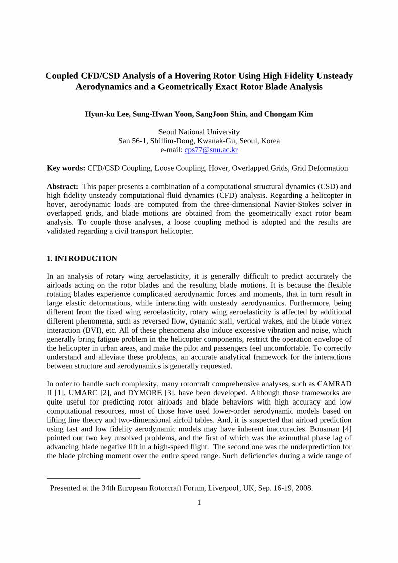
The computation results show good agreements with the experimental data for both validation cases as shown in Figure 5~7 and Table 3. Figure 6 and 7 shows Cp distributions on blade surface for 8° collective. Although viscous effect is not included in this test, it is seen that the present results compare well with the experimental measurements at all the radial locations for two different tip Mach numbers. Table 3 shows comparison of the thrust coefficient. The present error between CFD calculation and experimental data is less than 10%, which is comparable with the results of the other researchers.

9

Case 1 : Mtip = 0.439, θt = 8°

x/c

-Cp

0 0.2 0.4 0.6 0.8

-1

-0.5

0

0.5

1

Present (Inviscid)Experiment (C&T)

r/R=0.50

x/c

-Cp

0 0.2 0.4 0.6 0.8

-1

-0.5

0

0.5

1Present (Inviscid)Experiment (C&T)

r/R=0.68

x/c

-Cp

0 0.2 0.4 0.6 0.8

-1

-0.5

0

0.5

1Present (Inviscid)Experiment (C&T)

r/R=0.80

x/c

-Cp

0 0.2 0.4 0.6 0.8

-1

-0.5

0

0.5

1Present (Inviscid)Experiment (C&T)

r/R=0.89

x/c

-Cp

0 0.2 0.4 0.6 0.8

-1

-0.5

0

0.5

1Present (Inviscid)Experiment (C&T)

r/R=0.96

Figure 6 CP comparison result with the experimental data (Case 1)

Case 2 : Mtip = 0.877, θt = 8°

x/c

-Cp

0 0.2 0.4 0.6 0.8

-1

-0.5

0

0.5

1Present (Inviscid)Experiment (C&T)

r/R=0.50

x/c

-Cp

0 0.2 0.4 0.6 0.8

-1

-0.5

0

0.5

1Present (Inviscid)Experiment (C&T)

r/R=0.68

x/c

-Cp

0 0.2 0.4 0.6 0.8

-1

-0.5

0

0.5

1Present (Inviscid)Experiment (C&T)

r/R=0.80

x/c

-Cp

0 0.2 0.4 0.6 0.8

-1

-0.5

0

0.5

1Present (Inviscid)Experiment (C&T)

r/R=0.89

x/c

-Cp

0 0.2 0.4 0.6 0.8

-1

-0.5

0

0.5

1Present (Inviscid)Experiment (C&T)

r/R=0.96

Figure 7 CP comparison result with the experimental data (Case 2)

10

Figure 8 Isosurface and contour of cross-velocity (Case 2)

Table 3 Comparison of the thrust coefficient Experiment (C&T) Present (Inviscid)

Case 1 0.00459 0.00487

Case 2 0.00473 0.00528

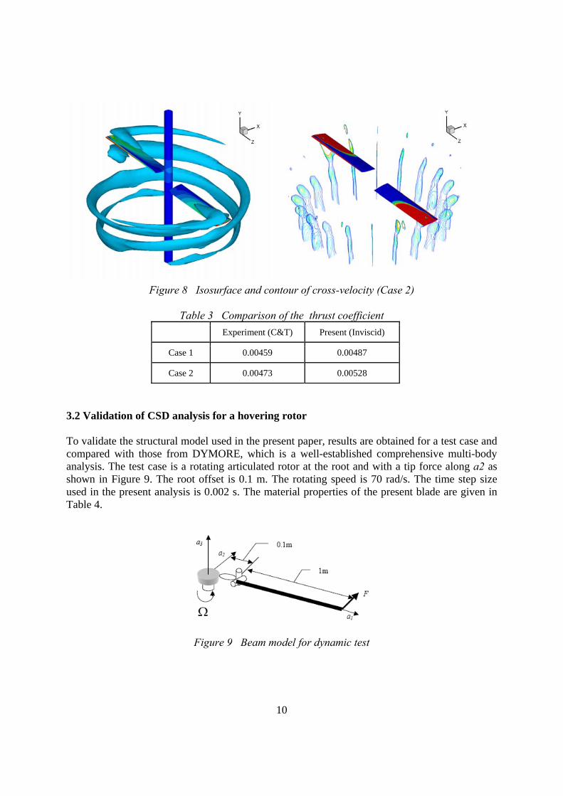
3.2 Validation of CSD analysis for a hovering rotor To validate the structural model used in the present paper, results are obtained for a test case and compared with those from DYMORE, which is a well-established comprehensive multi-body analysis. The test case is a rotating articulated rotor at the root and with a tip force along a2 as shown in Figure 9. The root offset is 0.1 m. The rotating speed is 70 rad/s. The time step size used in the present analysis is 0.002 s. The material properties of the present blade are given in Table 4.

Figure 9 Beam model for dynamic test

11

Table 4 Material properties of the test beam

Mass per unit span 0.2 kg/m Ixx 10-4 kg.m Iyy 10-6 kg.m Izz 10-4 kg.m K11 106 N K22 1020 N K33 1020 N K44 50 N.m2 K55 50 N.m2 K66 1000 N.m2

Figures 10 and 11 present the comparisons for the tip displacements and rotations with applied tip force of 1.0 sin 20t N. The results of the present analysis correlate well with those from DYMORE.

Figure 10 Comparison for the tip displacement Figure 11 Comparison for the tip rotation

3.3 CFD-CSD coupling analysis for a hovering rotor. Flight test or experimental data is quite rare for a CFD-CSD coupling analysis for hover. The only aircraft which reveals experimental hover data is UH-60A, and There is only one graph of validation available in Ref. [8] for that rotor. Table 5 is summary of the overset grid system for UH-60A rotor. Figure 12 shows typical plots of surface pressure distribution for the model UH60 blade at several spanwise stations, and the contours of pressure and cross velocity are given in Figure 13. Although the model hover tests were performed with a certain configuration and a few results were published for the UH-60 rotor, almost of the experimental data remains undisclosed. Thus, we survey for experimental data in the literature. In addition, since the blade geometry of UH-60A is not completely disclosed, there is some uncertainty in the blade modeling. In spite of those restrictions, the numerical results appear to be in a good agreement with the given data at the most spanwise stations. Discrepancy between the present analyses and experimental data is originated from the different blade geometry.

12

Table 5 Summary of the overset grid systems for UH-60A rotor

Blade Grid Background Grid

Type C-O type (round tip) H-type

Outer Boundary 2c~3c 5R(=76c)

Grid Points 85x41x163 = 568,055 On chord: 90 points On span : 60 points

80x90x104 = 748,800

x/c

Cp

0 0.2 0.4 0.6 0.8 1

-4

-3

-2

-1

0

1

ExpPresent(viscous)

r/R=0.225

x/c

Cp

0 0.2 0.4 0.6 0.8 1

-2

-1

0

1

2

ExpPresent(viscous)

r/R=0.550

x/c

Cp

0 0.2 0.4 0.6 0.8 1

-2

-1

0

1

2

ExpPresent(viscous)

r/R=0.775

x/c

Cp

0 0.2 0.4 0.6 0.8 1

-2

-1

0

1

2

ExpPresent(viscous)

r/R=0.865

x/c

Cp

0 0.2 0.4 0.6 0.8 1

-2

-1

0

1

2

ExpPresent(viscous)

r/R=0.920

x/c

Cp

0 0.2 0.4 0.6 0.8 1

-2

-1

0

1

2

ExpPresent(viscous)

r/R=0.965

Figure 12 CP comparison result with the experimental data for UH-60A rotor

Figure 13 Contour of the blade surface pressure and the cross-velocity in UH-60A

13

r/R0 0.2 0.4 0.6 0.8 1

0

0.05

0.1

0.15

0.2

c9605OVERFLOW/CAMRADCAMRAD free wakePresent

Figure 14 Mean normal force distribution of a UH-60A rotor in hover

Figure 15 shows the mean vertical force distribution of a UH-60A rotor in hover, which is an intermediate validation target for the CFD-CSD analysis in Ref. 8. In the region of / 0.7r R ≤ , the present result is quite comparable with the others. However, there are in general significant discrepancy between the present results and experimental data. From the results in the previous research, it is observed to be difficult to match accurately the results to experimental data near the blade tip. Nevertheless, a general improvement is required for the present analysis and its results will be illustrated in the future paper of the authors. 3. CONCLUDING REMARKS A CFD/CSD coupled analysis is conducted for a hovering helicopter. A three-dimensional unsteady Navier-Stokes CFD solver and one-dimensional geometrically exact rotor beam CSD analyses are established and validated independently. Using a UH-60A hovering flight test data, preliminary results are obtained for the present CFD/CSD coupled research. It is observed that further improvement is required for the present approach. After such improvement is completed for a hover condition, forward flight analysis will be pursued regarding HART-II configuration. ACKNOWLEDGEMENTS This study was supported by the Korea Aerospace Research Institute under Korean Helicopter Program Dual-Use Component Development Project, which is further funded by the Korean Ministry of Knowledge and Economics. And this research has also been supported by the Institute of Advanced Aerospace Technology in Seoul National University, Korea.

14

REFERENCES [1] Johnson, W., “CAMRAD II, Comprehensive Analytical Model of Rotorcraft

Aerodynamics and Dynamics,” Johnson Aeronautics, Palo Alto, California, 1992-1997. [2] Bir, G., Chopra, I., and et al. “University of Maryland Advanced Rotor Code (UMARC)

Theory Manual,” Technical Report UM-AERO 94-18, Center for Rotorcraft Education and Research, University of Maryland, College Park, July 1994.

[3] Bauchau, O. A., “DYMORE Users’ Manual,” School of Aerospace Engineering, Georgia Institute of Technology, Atlanta, GA, May 2006.

[4] Bousman, W. G., “Putting the Aero Back into Aeroelasticity,” 8th ARO Workshop on Aeroelasticity of Rotorcraft Systems, University Park, PA, October 1999.

[5] Nguyen, K. and Johnson, W., “Evaluation of Dynamic Stall Models with Flight Test Data,” American Helicopter Society 54th Annual Forum, Washington, D.C., May 1998.

[6] Lim, J. W., and Anastassiades, T., “Correlation of 2GCHAS Analysis with Experimental Data,” Journal of the American Helicopter Society, Vol. 40, No. 4, October 1995, pp. 18-33.

[7] Yeo, H. and Johnson, W., “Assessment of Comprehensive Analysis Calculation on Helicopter Rotors,” American Helicopter Society 4th Decennial Specialists’ Conference on Aeromechanics, San Francisco, CA, January 2004.

[8] Potsdam, M., Yeo, H., and Johnson, W., “Rotor Airloads Prediction using Loose Aerodynamic/Structural Coupling,” American Helicopter Society 60th Annual Forum, Baltimore, MD, June 7-10, 2004.

[9] Sitaraman, J., Datta, A., Chopra, I., and Baeder, J., “Prediction of Rotor Aerodynamic and Structural Loads using CFD/CSD Coupling at Three Critical Level Flight Conditions,” 31st European Rotorcraft Forum, Florence, Italy, September 2005.

[10] Tung, C., Gallman, J.M., Kube, R., Wagner, W., van der Wall, B., Brooks, T.F., Burley, C.L., Boyd, D. D., Rahier, G., and Beaumier, P., “Prediction and Measurement of Blade-Vortex Interaction Loading,” 1st Joint CEAS/AIAA Aeroacoustics Conference Proceedings, Munich, Germany, June 1995.

[11] Lim, J. W., and Strawn, R. C., “Computational Modeling of HART II Blade-Vortex Interaction Loading and Wake System,” Journal of Aircraft, Vol. 45, No. 3, 2008, pp. 923-933.

[12] Yang, C., Inada, Y., and Aoyama, T., “BVI Noise Prediction Using HART II Motion Data,” International Forum of Rotorcraft Multidisciplinary Technology Proceedings, Seoul, Korea, October 2007.

[13] Tanabe, Y., and Saito, S., “A Simple CFD/CSD Loose Coupling Approach for Rotor Blade Aeroelasticity,” 33rd European Rotorcraft Forum, Kazan, Russia, September 11-13, 2007.

[14] Lim, J. W., “An Assessment of Rotor Dynamics Correlation for Descending Flight Using CFD/CSD Coupled Analysis,” American Helicopter Society 64th Annual Forum, Montreal, Canada, April 29-May 1, 2008.

[15] Tung, C., Caradonna, F. X., and Johnson, W. R., “The Prediction of Transonic Flows on an Advancing Rotor,” Journal of the American Helicopter Society, Vol. 31, No. 3, July 1986.

[16] Srinivasan, G.R., and Baeder, J.D., “TURNS: A Free-wake Euler/ Navier-Stokes Numerical Method for Helicopter Rotors,” AIAA Journal, Vol. 31, No. 5, 1993.

15

[17] Roe, P. L., “Approximate Riemann Solvers, Parameter Vectors, and Difference Schemes,” Journal of Computational Physics, Vol. 43, No. 3, 1981, pp. 357-372.

[18] Van Leer, B., “Towards the Ultimate Conservative Difference Scheme V. A Second Order Sequel to Godunov's Method,” Journal of Computational Physics, Vol. 32, 1979.

[19] Jameson, A., and Yoon, S., “Lower-Upper Implicit Schemes with Multiple Grids for the Euler Equations,” AIAA Journal, Vol. 25, No. 7, 1987, pp. 929-935.

[20] Yoon, S., and Jameson, A., “An LU-SSOR Scheme for the Euler and Navier-Stokes Equations,” AIAA Paper 87-0600, January 1987.

[21] Baldwin, B. S. and Lomax, H., “Thin Layer Approximation and Algebraic Model for Separated Turbulent Flow,” AIAA Paper 78-0257, AIAA 16th Aerospace Sciences Meeting, Huntsville, Alabama, January 1978.

[22] Xueqiang Liu, Ning Qin and Hao Xia, “Fast dynamic grid deformation based on Delaunay graph mapping,” Journal of Computational Physics, Vol. 211, 2006, pp. 405–423.

[23] Hodges, D. H, “A Mixed Variational Formulation based on Exact Intrinsic Equations for Dynamics of Moving Beams,” International Journal of Solids and Structures, Vol. 25, No. 11, 1990.

[24] Shang, X., “Aeroelastic Stability of Composite Hingeless Rotors with Finite-State Unsteady Aerodynamics,” Ph.D. Dissertation, Georgia Institute of Technology, August 1995.

[25] Cheng, T., “Structural Dynamics Modeling of Helicopter Blades for Computational Aeroelasticity,” M.S. Thesis, Massachusetts Institute of Technology, May, 2002.

[26] Kim, K., “The Effect of the Blade Nonlinear Deflection upon Fluid-Structure Interaction Analysis in Helicopters,” M.S. Thesis, Seoul National University, 2007.

[27] Caradonna, F. X., and Tung, C., “Experimental and Analytical Studies of a Model Helicopter Rotor in Hover,” NASA TM 81232, 1981.