Coupled Flight Dynamics and CFD Analysis of Pilot Workload ... · Coupled Flight Dynamics and CFD...

American Institute of Aeronautics and Astronautics

1

Coupled Flight Dynamics and CFD Analysis of Pilot Workload in Ship Airwakes

Derek O. Bridges,1 Joseph F. Horn,2 Emre Alpman,3 and Lyle N. Long4 The Pennsylvania State University, University Park, PA 16802

This paper describes a recent investigation of the helicopter/ship dynamic interface, in which pilot workload is examined using a novel coupling of flight dynamics and CFD analysis. This fully coupled method uses preexisting flight dynamics and CFD analysis codes, running concurrently; the two codes share data, with the flight dynamics code providing position and loading data and the CFD analysis code providing local velocity data. Results obtained using the fully coupled method are compared to results with no coupling, one-way coupling, where the flight dynamics code uses precalculated airwake solutions, and flight test data. Analysis of the time history and frequency domain results and the CFD solutions shows that the one-way coupling method can predict a level of pilot workload equal to or greater than that of the fully coupled method for the cases simulated. The addition of the rotor downwash to the CFD solution in the fully coupled method shows that vortices in the airwake that have a significant effect in one-way coupling may have either a similar effect or a lessened effect if the vortices are pushed away from the helicopter.

I. Background hipboard operation of rotorcraft remains a topic of significant interest to both civilian and military operators, particularly in the launch and recovery regimes where the rotorcraft is in close proximity to the ship and its

resultant airwake. Due to the combination of a moving ship deck and an unsteady, highly turbulent ship airwake, pilot workload for a rotorcraft operating in the vicinity of a ship can be very high, as shown in numerous simulation studies.1-5 However, in these studies (as well as numerous others for various types of ships, including amphibious assault ships6-8, aircraft carriers9, and destroyers10,11), the flowfield of the ship airwake is precalculated using a model based on CFD analysis; thus the flow is not affected by the presence of the rotorcraft. This one-way coupling of the aerodynamic interactions between the downwash of the rotorcraft and the ship airwake is somewhat questionable due to the nonlinear, unsteady nature of both the ship airwake and rotorcraft dynamics, which invalidates the principle of superposition. Other research efforts have examined the effects of unsteady airwakes on pilot workload by analyzing flight test data12,13 or wind tunnel tests14,15, but these analyses cannot be used as a prediction tool for the design of new rotorcraft or ships. Still other projects have taken preliminary steps towards understanding the aerodynamic coupling the effects between the ship airwake and an aircraft; one paper details the coupling of a ship airwake from an LHA-class amphibious assault ship with the jet downwash from a hovering AV-8B Harrier16, while another analyzes the coupling between an LHA airwake and the rotor wash of a hovering V-22 Osprey, in which the rotors are modeled as actuator disks17. In both of these studies, the aircraft position was specified and the flight dynamics and pilot compensation were modeled.

Recently, a method has been developed to simulate the fully coupled aerodynamic ship/helicopter dynamic interface.18 In this method, flight dynamics simulation and CFD analysis software are run concurrently with communication between the two so that the effect of the ship airwake on the rotorcraft as well as the effect of the rotorcraft on the ship airwake can be calculated. This fully coupled method cannot run in real-time (as some of the one-way coupling methods have in order to be used in piloted simulation) due to the computational requirements of the CFD analysis, but still provides useful results that are important in determining the effects of coupling on the rotorcraft pilot workload.

1 Graduate Research Assistant, Department of Aerospace Engineering, Student Member, AIAA. 2 Associate Professor, Department of Aerospace Engineering, AIAA Associate Fellow. 3 Assistant Professor, Mechanical Engineering Department, Marmara University, Istanbul, Turkey, Member, AIAA. 4 Distinguished Professor, Department of Aerospace Engineering, AIAA Fellow.

S

LNL

Text Box

AIAA Paper No. 2007-6485, Presented at AIAA Atmospheric Flight Dynamics Conference, Hilton Head, SC, Aug., 2007


2

II. Objective In this paper, the effects of the coupled ship/rotorcraft aerodynamic environment on pilot workload will be

examined. Specifically, three different models of the aerodynamic environment will be analyzed: 1. No coupling (no airwake model). 2. One-way coupling. 3. Full coupling. In the no coupling case, only a constant wind is included in the flight dynamics simulation; the CFD calculations

are not used. Instead, the flight dynamics code computes the rotor downwash using the Pitt-Peters inflow model.19 Ground effect is included in the model, although atmospheric turbulence effects are not included. For the one-way coupling case, the ship airwake is calculated a priori using CFD analysis of the flow field around the ship without the rotorcraft present. The airwake data is then stored and later incorporated into the flight dynamics code as external disturbances; these external disturbances then affect the local velocities at each of the rotorcraft components (main rotor blade elements, tail rotor, fuselage, empennage, etc.), which in turn affect the total forces and moments on the rotorcraft. Thus, the effects of the ship airwake on the rotorcraft response are simulated, but the effects of the rotorcraft on the ship airwake are ignored.

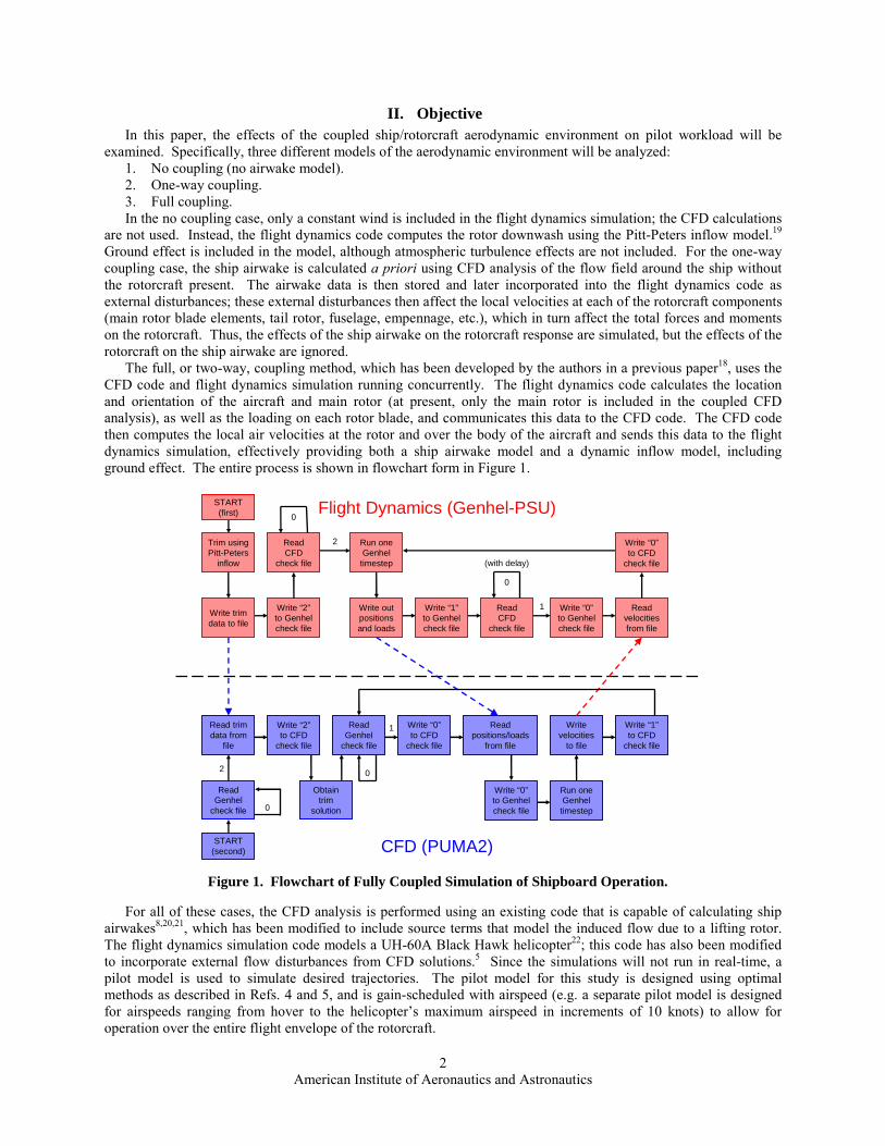
The full, or two-way, coupling method, which has been developed by the authors in a previous paper18, uses the CFD code and flight dynamics simulation running concurrently. The flight dynamics code calculates the location and orientation of the aircraft and main rotor (at present, only the main rotor is included in the coupled CFD analysis), as well as the loading on each rotor blade, and communicates this data to the CFD code. The CFD code then computes the local air velocities at the rotor and over the body of the aircraft and sends this data to the flight dynamics simulation, effectively providing both a ship airwake model and a dynamic inflow model, including ground effect. The entire process is shown in flowchart form in Figure 1.

For all of these cases, the CFD analysis is performed using an existing code that is capable of calculating ship

airwakes8,20,21, which has been modified to include source terms that model the induced flow due to a lifting rotor. The flight dynamics simulation code models a UH-60A Black Hawk helicopter22; this code has also been modified to incorporate external flow disturbances from CFD solutions.5 Since the simulations will not run in real-time, a pilot model is used to simulate desired trajectories. The pilot model for this study is designed using optimal methods as described in Refs. 4 and 5, and is gain-scheduled with airspeed (e.g. a separate pilot model is designed for airspeeds ranging from hover to the helicopter’s maximum airspeed in increments of 10 knots) to allow for operation over the entire flight envelope of the rotorcraft.

(with delay)

Trim using Pitt-Peters

inflow

Write trim data to file

Write “2”to Genhelcheck file

Run one Genhel

timestep

Write out positions and loads


Read CFD

check file

Read velocities from file

Read Genhel

check file

Read trim data from

file

Obtain trim

solution

Run one Genhel

timestep

Read Genhel

check file

Write velocities

to file

Write “1”to CFD

check file


Write “0”to CFD

check file

Read positions/loads

from file

Flight Dynamics (Genhel-PSU)

CFD (PUMA2)

2

1

0

1

0

0

Write “2”to CFD

check file

Read CFD

check file

0

2

START (first)

START (second)

Write “0”to CFD

check file


Figure 1. Flowchart of Fully Coupled Simulation of Shipboard Operation.


3

III. CFD Methodology In this study, viscous effects were neglected and Euler equations were used to define the flowfield. Rotor

modeling was performed using momentum sources which were added to momentum and energy equations. The magnitudes of these source terms were computed using the loads obtained from the flight dynamics code. Numerical solutions were obtained by modifying the in-house computational fluid dynamics code PUMA2. In order to reduce the CPU time and memory requirements parallel processing with MPI was used.23 PUMA2 uses a finite volume method to discretize the governing equations. The effect of the rotor has been included in each computational cell as a force-per-unit volume term. This model does not require a well-defined rotor plane inside the computational mesh; therefore, source terms can be easily moved inside the domain to simulate rotor motion. The method can also be used for more than one rotor simultaneously, allowing for analysis of multiple rotors. PUMA2 was also modified to include atmospheric boundary layer and atmospheric turbulence effects which may be important when the rotorcraft is in ground effect or in the vicinity of a ship.

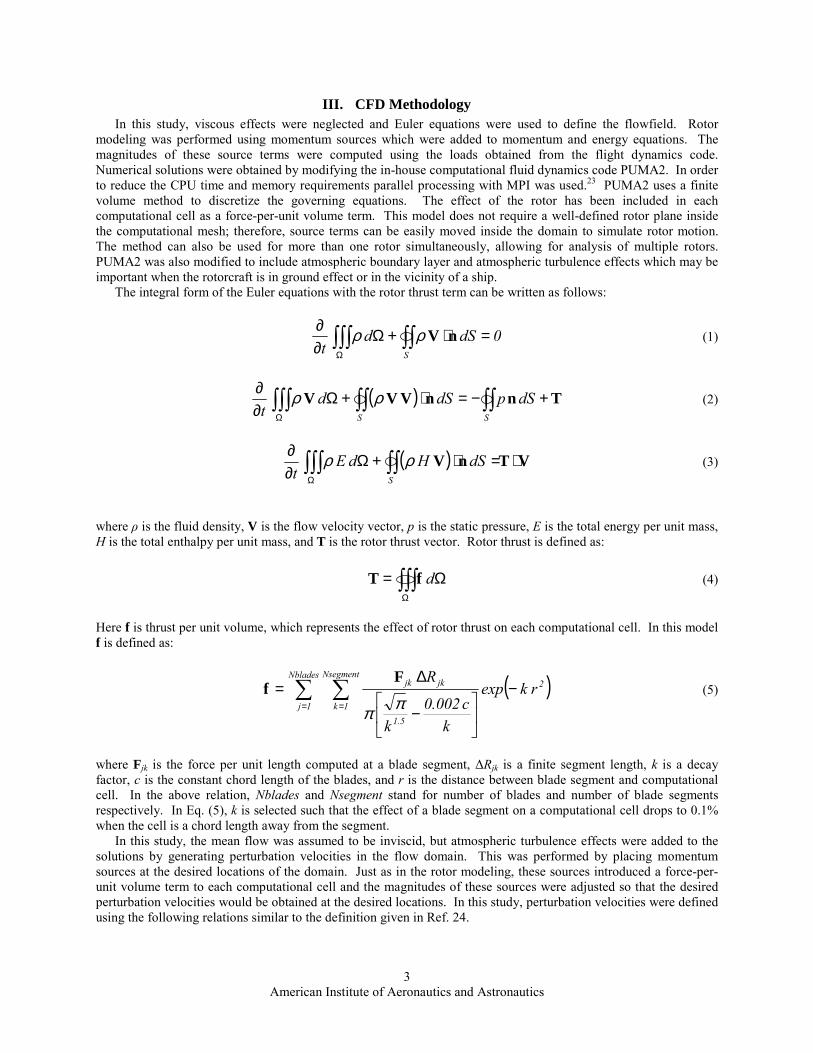
The integral form of the Euler equations with the rotor thrust term can be written as follows:

∫∫∫∫∫ =⋅+Ω∂∂

Ω S

0dSdt

nVρρ (1)

( ) TnnVVV +−=⋅+Ω∂∂

∫∫ ∫∫∫∫∫Ω S S

dSpdSdt

ρρ (2)

( ) VTnV ⋅=⋅+Ω∂∂

∫∫∫∫∫Ω S

dSHdEt

ρρ (3)

where ρ is the fluid density, V is the flow velocity vector, p is the static pressure, E is the total energy per unit mass, H is the total enthalpy per unit mass, and T is the rotor thrust vector. Rotor thrust is defined as:

∫∫∫Ω

Ω= dfT (4)

Here f is thrust per unit volume, which represents the effect of rotor thrust on each computational cell. In this model f is defined as:

( )2Nblades

1j

Nsegment

1k5.1

jkjk rkexp

kc002.0

k

R−

−

∆= ∑ ∑

= = ππ

Ff (5)

where Fjk is the force per unit length computed at a blade segment, ∆Rjk is a finite segment length, k is a decay factor, c is the constant chord length of the blades, and r is the distance between blade segment and computational cell. In the above relation, Nblades and Nsegment stand for number of blades and number of blade segments respectively. In Eq. (5), k is selected such that the effect of a blade segment on a computational cell drops to 0.1% when the cell is a chord length away from the segment.

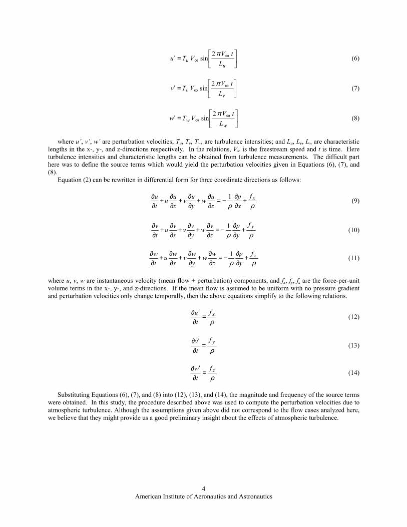
In this study, the mean flow was assumed to be inviscid, but atmospheric turbulence effects were added to the solutions by generating perturbation velocities in the flow domain. This was performed by placing momentum sources at the desired locations of the domain. Just as in the rotor modeling, these sources introduced a force-per-unit volume term to each computational cell and the magnitudes of these sources were adjusted so that the desired perturbation velocities would be obtained at the desired locations. In this study, perturbation velocities were defined using the following relations similar to the definition given in Ref. 24.


4

=′ ∞

∞u

u LtV

VTuπ2

sin (6)

=′ ∞

∞v

v LtV

VTvπ2

sin (7)

=′ ∞

∞w

w LtV

VTwπ2

sin (8)

where u’, v’, w’ are perturbation velocities; Tu, Tv, Tw, are turbulence intensities; and Lu, Lv, Lw are characteristic lengths in the x-, y-, and z-directions respectively. In the relations, V∞ is the freestream speed and t is time. Here turbulence intensities and characteristic lengths can be obtained from turbulence measurements. The difficult part here was to define the source terms which would yield the perturbation velocities given in Equations (6), (7), and (8).

Equation (2) can be rewritten in differential form for three coordinate directions as follows:

ρρxf

xp

zuw

yuv

xuu

tu +

∂∂

−=∂∂+

∂∂+

∂∂+

∂∂ 1 (9)

ρρyf

yp

zvw

yvv

xvu

tv +

∂∂

−=∂∂+

∂∂+

∂∂+

∂∂ 1 (10)

ρρzf

yp

zww

ywv

xwu

tw +

∂∂

−=∂∂+

∂∂+

∂∂+

∂∂ 1 (11)

where u, v, w are instantaneous velocity (mean flow + perturbation) components, and fx, fy, fz are the force-per-unit volume terms in the x-, y-, and z-directions. If the mean flow is assumed to be uniform with no pressure gradient and perturbation velocities only change temporally, then the above equations simplify to the following relations.

ρxf

tu =∂

′∂ (12)

ρyf

tv =

∂′∂ (13)

ρzf

tw =∂

′∂ (14)

Substituting Equations (6), (7), and (8) into (12), (13), and (14), the magnitude and frequency of the source terms were obtained. In this study, the procedure described above was used to compute the perturbation velocities due to atmospheric turbulence. Although the assumptions given above did not correspond to the flow cases analyzed here, we believe that they might provide us a good preliminary insight about the effects of atmospheric turbulence.


5

IV. Results

A. Hangar Airwake Hover Results In order to examine the effects of airwake coupling on pilot workload, it is helpful to first compare the

simulation results against flight test data. For this study, the baseline case was described in Reference 12, in which a UH-60A helicopter hovers in the airwake produced by a 16-knot wind passing over an aircraft hangar at San Francisco International Airport. The case of a UH-60A hovering in the hangar airwake was also previously analyzed in Ref. 18; however, atmospheric turbulence was not included in the CFD solution. The numerical solutions presented there did not generate the expected unsteady disturbances.18 Therefore, in this study, atmospheric turbulence effects were introduced to the flowfield by placing momentum sources along a vertical plane passing through the front face of the hangar. Turbulence was assumed to isotropic in that the turbulence intensity is same in all directions. Turbulence intensity value and characteristic lengths were taken from Ref. 25.

Three runs of this hover case were simulated: one run with no airwake coupling, one run with one-way airwake coupling, and one run with full CFD/flight dynamics coupling. For the three simulated cases, the helicopter was initially located at the top rear of the CFD grid; a defined trajectory was used to have the helicopter descend and move forward from its starting location to the point of interest 100 feet away the hangar at an altitude of 35.5 feet (which puts the rotor disk at approximately the same altitude as the roof of the hangar). This approach and descent trajectory was chosen so that the rotor wake would not affect the initial formation of vortices at the front of the hangar. In the time history results shown below, only the hover portion of the maneuver (beginning at 15 seconds) is included. Actual flight test data from Ref. 12 is included with the simulation results for comparison.

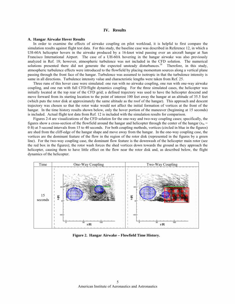
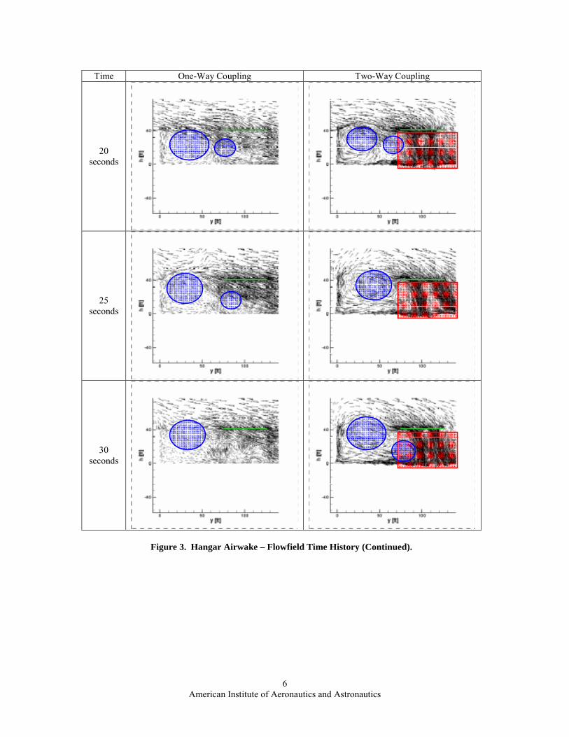
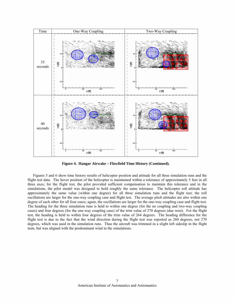
Figures 2-4 are visualizations of the CFD solution for the one-way and two-way coupling cases; specifically, the figures show a cross-section of the flowfield around the hangar and helicopter through the center of the hangar (xN = 0 ft) at 5-second intervals from 15 to 40 seconds. For both coupling methods, vortices (circled in blue in the figures) are shed from the cliff-edge of the hangar shape and move away from the hangar. In the one-way coupling case, the vortices are the dominant feature of the flow in the region of the rotor disk (represented in the figures by a green line). For the two-way coupling case, the dominant flow feature is the downwash of the helicopter main rotor (see the red box in the figures); the rotor wash forces the shed vortices down towards the ground as they approach the helicopter, causing them to have little effect on the flow near the rotor disk and, as described below, the flight dynamics of the helicopter.

Time One-Way Coupling Two-Way Coupling

15 seconds

Figure 2. Hangar Airwake – Flowfield Time History.


6


20 seconds

25 seconds

30 seconds

Figure 3. Hangar Airwake – Flowfield Time History (Continued).


7

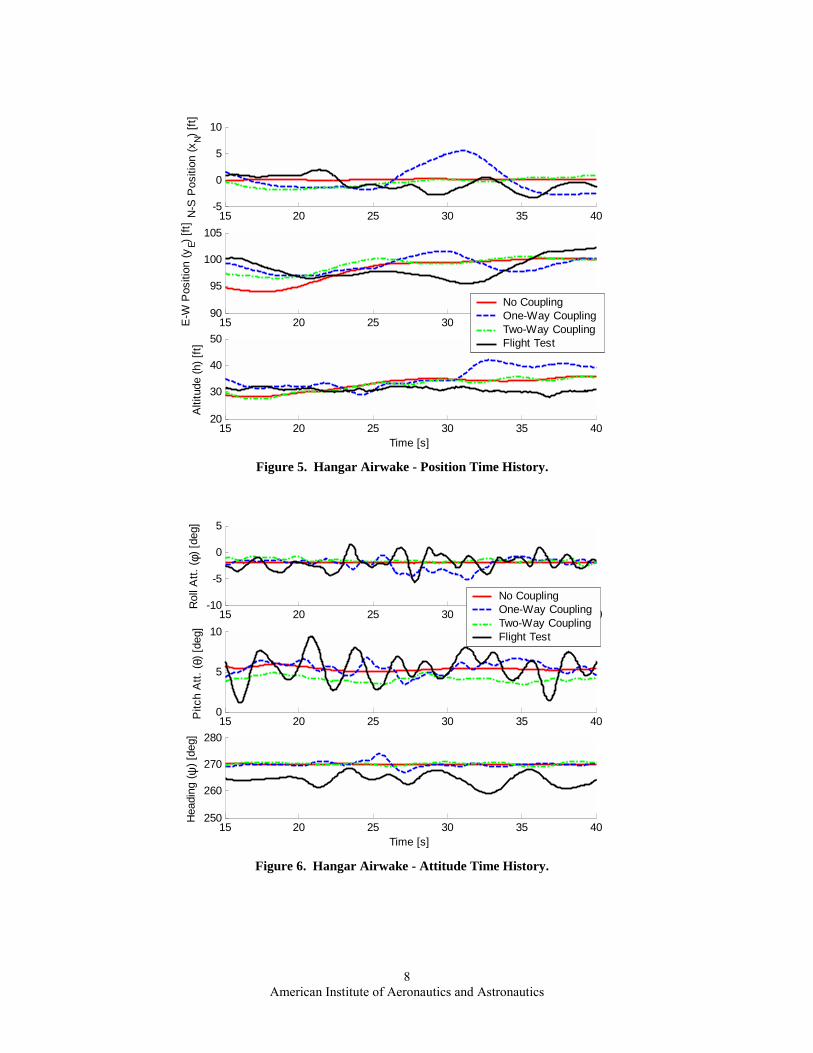
Figures 5 and 6 show time history results of helicopter position and attitude for all three simulation runs and the

flight test data. The hover position of the helicopter is maintained within a tolerance of approximately 5 feet in all three axes; for the flight test, the pilot provided sufficient compensation to maintain this tolerance and in the simulations, the pilot model was designed to hold roughly the same tolerance. The helicopter roll attitude has approximately the same value (within one degree) for all three simulation runs and the flight test; the roll oscillations are larger for the one-way coupling case and flight test. The average pitch attitudes are also within one degree of each other for all four cases; again, the oscillations are larger for the one-way coupling case and flight test. The heading for the three simulation runs is held to within one degree (for the no coupling and two-way coupling cases) and four degrees (for the one-way coupling case) of the trim value of 270 degrees (due west). For the flight test, the heading is held to within four degrees of the trim value of 264 degrees. The heading difference for the flight test is due to the fact that the wind direction during the flight test was reported as 260 degrees, not 270 degrees, which was used in the simulation runs. Thus the aircraft was trimmed in a slight left sideslip in the flight tests, but was aligned with the predominant wind in the simulations.


35 seconds

40 seconds

Figure 4. Hangar Airwake – Flowfield Time History (Continued).


8

15 20 25 30 35 40-10

-5

0

5

Rol

l Att.

( φ) [

deg]

15 20 25 30 35 400

5

10

Pitc

h A

tt. ( θ

) [de

g]

15 20 25 30 35 40250

260

270

280

Hea

ding

( ψ) [

deg]

Time [s]

No Coupling One-Way CouplingTwo-Way CouplingFlight Test

Figure 6. Hangar Airwake - Attitude Time History.

15 20 25 30 35 40-5

0

5

10

N-S

Pos

ition

(xN) [

ft]

15 20 25 30 35 4090

95

100

105

E-W

Pos

ition

(yE) [

ft]

15 20 25 30 35 4020

30

40

50

Alti

tude

(h) [

ft]

Time [s]

No Coupling One-Way CouplingTwo-Way CouplingFlight Test

Figure 5. Hangar Airwake - Position Time History.


9

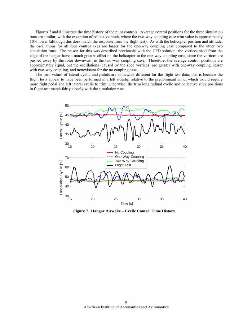
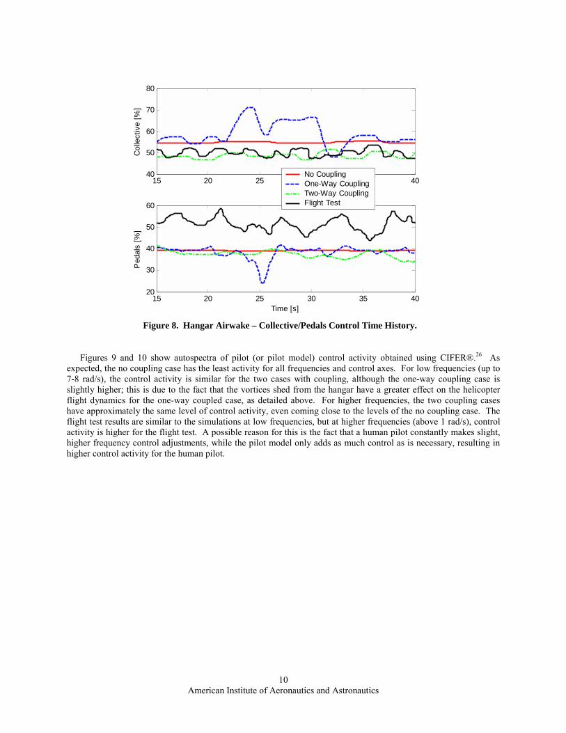
Figures 7 and 8 illustrate the time history of the pilot controls. Average control positions for the three simulation runs are similar, with the exception of collective pitch, where the two-way coupling case trim value is approximately 10% lower (although this does match the response from the flight test). As with the helicopter position and attitude, the oscillations for all four control axes are larger for the one-way coupling case compared to the other two simulation runs. The reason for this was described previously with the CFD solution; the vortices shed from the edge of the hangar have a much greater effect on the helicopter in the one-way coupling case, since the vortices are pushed away by the rotor downwash in the two-way coupling case. Therefore, the average control positions are approximately equal, but the oscillations (caused by the shed vortices) are greater with one-way coupling, lesser with two-way coupling, and nonexistent for the no coupling case.

The trim values of lateral cyclic and pedals are somewhat different for the flight test data; this is because the flight tests appear to have been performed in a left sideslip relative to the predominant wind, which would require more right pedal and left lateral cyclic to trim. Otherwise, the trim longitudinal cyclic and collective stick positions in flight test match fairly closely with the simulation runs.

15 20 25 30 35 4030

35

40

45

50

Late

ral C

yclic

[%]

15 20 25 30 35 4030

40

50

60

70

Long

itudi

nal C

yclic

[%]

Time [s]

No CouplingOne-Way CouplingTwo-Way CouplingFlight Test

Figure 7. Hangar Airwake – Cyclic Control Time History.


10

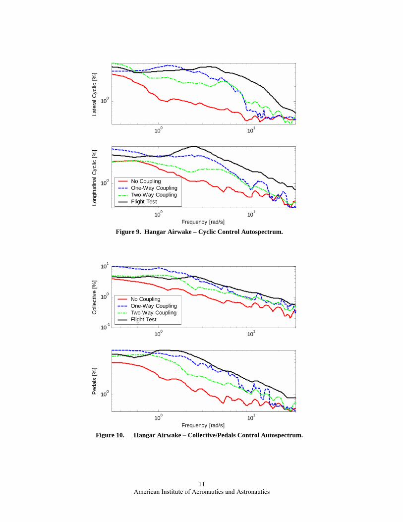
Figures 9 and 10 show autospectra of pilot (or pilot model) control activity obtained using CIFER®.26 As

expected, the no coupling case has the least activity for all frequencies and control axes. For low frequencies (up to 7-8 rad/s), the control activity is similar for the two cases with coupling, although the one-way coupling case is slightly higher; this is due to the fact that the vortices shed from the hangar have a greater effect on the helicopter flight dynamics for the one-way coupled case, as detailed above. For higher frequencies, the two coupling cases have approximately the same level of control activity, even coming close to the levels of the no coupling case. The flight test results are similar to the simulations at low frequencies, but at higher frequencies (above 1 rad/s), control activity is higher for the flight test. A possible reason for this is the fact that a human pilot constantly makes slight, higher frequency control adjustments, while the pilot model only adds as much control as is necessary, resulting in higher control activity for the human pilot.

15 20 25 30 35 4040

50

60

70

80

Col

lect

ive

[%]

15 20 25 30 35 4020

30

40

50

60

Ped

als

[%]

Time [s]


Figure 8. Hangar Airwake – Collective/Pedals Control Time History.


11

100 10110-1

100

101

Col

lect

ive

[%]

100 101

100

Frequency [rad/s]

Ped

als

[%]


Figure 10. Hangar Airwake – Collective/Pedals Control Autospectrum.

100 101

100La

tera

l Cyc

lic [%

]

100 101

100

Long

itudi

nal C

yclic

[%]

Frequency [rad/s]


Figure 9. Hangar Airwake – Cyclic Control Autospectrum.


12

B. LHA Approach Results The second series of airwake results is designed to replicate an actual maneuver performed by a rotorcraft

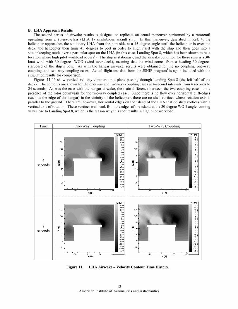
operating from a Tarawa-class (LHA 1) amphibious assault ship. In this maneuver, described in Ref. 4, the helicopter approaches the stationary LHA from the port side at a 45 degree angle until the helicopter is over the deck; the helicopter then turns 45 degrees to port in order to align itself with the ship and then goes into a stationkeeping mode over a particular spot on the LHA (in this case, Landing Spot 8, which has been shown to be a location where high pilot workload occurs1). The ship is stationary, and the airwake condition for these runs is a 30-knot wind with 30 degrees WOD (wind over deck), meaning that the wind comes from a heading 30 degrees starboard of the ship’s bow. As with the hangar airwake, results were obtained for the no coupling, one-way coupling, and two-way coupling cases. Actual flight test data from the JSHIP program4 is again included with the simulation results for comparison.

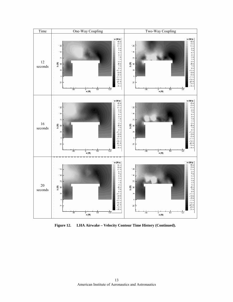
Figures 11-13 show vertical velocity contours on a plane passing through Landing Spot 8 (the left half of the deck). The contours are shown for the one-way and two-way coupling cases at 4-second intervals from 4 seconds to 24 seconds. As was the case with the hangar airwake, the main difference between the two coupling cases is the presence of the rotor downwash for the two-way coupled case. Since there is no flow over horizontal cliff-edges (such as the edge of the hangar) in the vicinity of the helicopter, there are no shed vortices whose rotation axis is parallel to the ground. There are, however, horizontal edges on the island of the LHA that do shed vortices with a vertical axis of rotation. These vortices trail back from the edges of the island at the 30-degree WOD angle, coming very close to Landing Spot 8, which is the reason why this spot results in high pilot workload.1


4 seconds

8 seconds

Figure 11. LHA Airwake – Velocity Contour Time History.


13


12 seconds

16 seconds

20 seconds

Figure 12. LHA Airwake – Velocity Contour Time History (Continued).


14

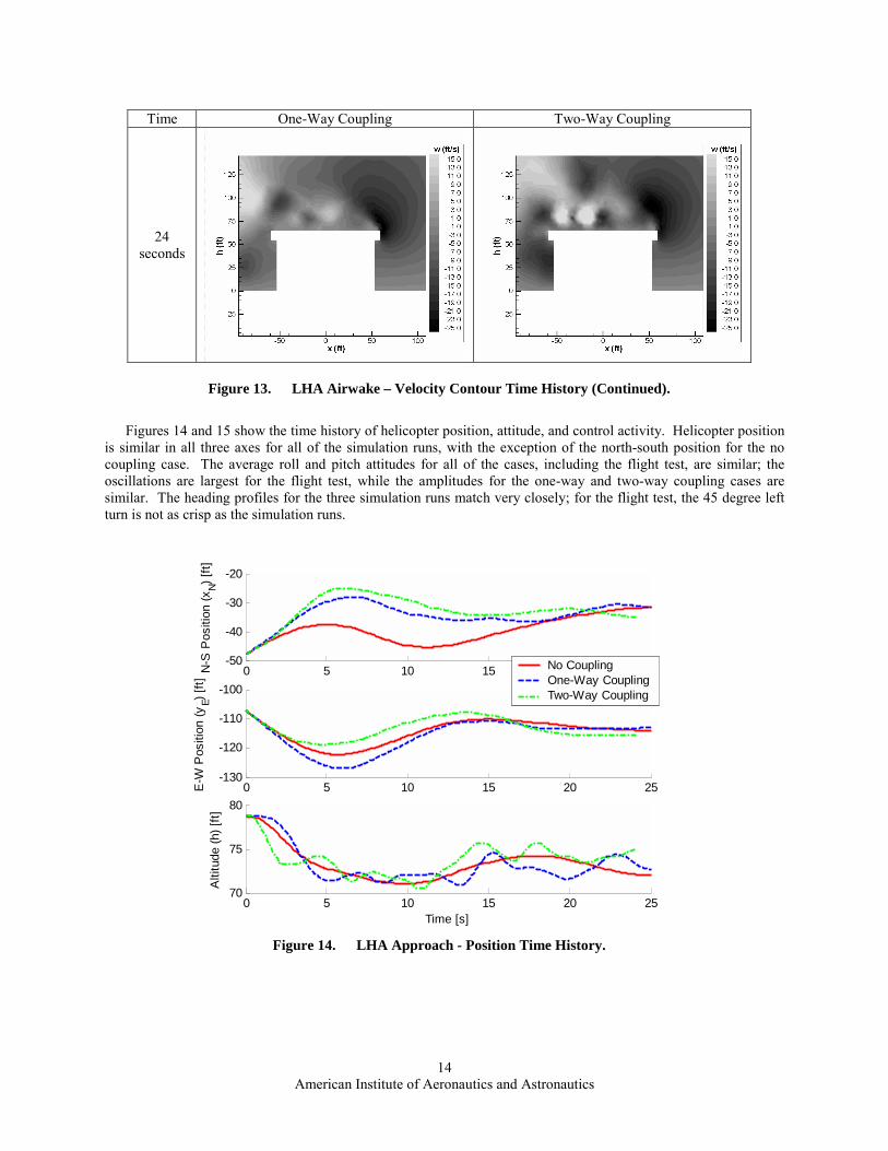
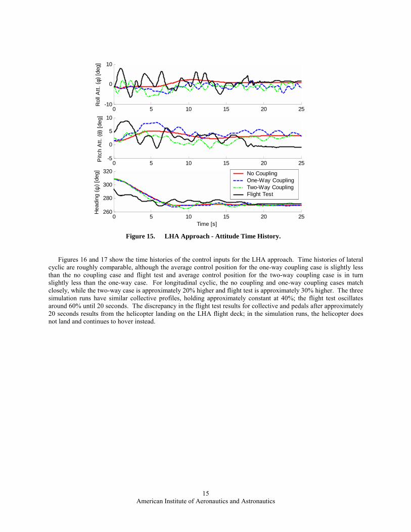
Figures 14 and 15 show the time history of helicopter position, attitude, and control activity. Helicopter position

is similar in all three axes for all of the simulation runs, with the exception of the north-south position for the no coupling case. The average roll and pitch attitudes for all of the cases, including the flight test, are similar; the oscillations are largest for the flight test, while the amplitudes for the one-way and two-way coupling cases are similar. The heading profiles for the three simulation runs match very closely; for the flight test, the 45 degree left turn is not as crisp as the simulation runs.


24 seconds

Figure 13. LHA Airwake – Velocity Contour Time History (Continued).

0 5 10 15 20 25-50

-40

-30

-20

N-S

Pos

ition

(xN) [

ft]

0 5 10 15 20 25-130

-120

-110

-100

E-W

Pos

ition

(yE) [

ft]

0 5 10 15 20 2570

75

80

Alti

tude

(h) [

ft]

Time [s]

No CouplingOne-Way CouplingTwo-Way Coupling

Figure 14. LHA Approach - Position Time History.


15

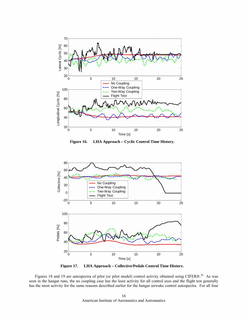
Figures 16 and 17 show the time histories of the control inputs for the LHA approach. Time histories of lateral

cyclic are roughly comparable, although the average control position for the one-way coupling case is slightly less than the no coupling case and flight test and average control position for the two-way coupling case is in turn slightly less than the one-way case. For longitudinal cyclic, the no coupling and one-way coupling cases match closely, while the two-way case is approximately 20% higher and flight test is approximately 30% higher. The three simulation runs have similar collective profiles, holding approximately constant at 40%; the flight test oscillates around 60% until 20 seconds. The discrepancy in the flight test results for collective and pedals after approximately 20 seconds results from the helicopter landing on the LHA flight deck; in the simulation runs, the helicopter does not land and continues to hover instead.

0 5 10 15 20 25-10

0

10

Rol

l Att.

( φ) [

deg]

0 5 10 15 20 25-5

0

5

10

Pitc

h A

tt. ( θ

) [de

g]

0 5 10 15 20 25260

280

300

320

Hea

ding

( ψ) [

deg]

Time [s]


Figure 15. LHA Approach - Attitude Time History.


16

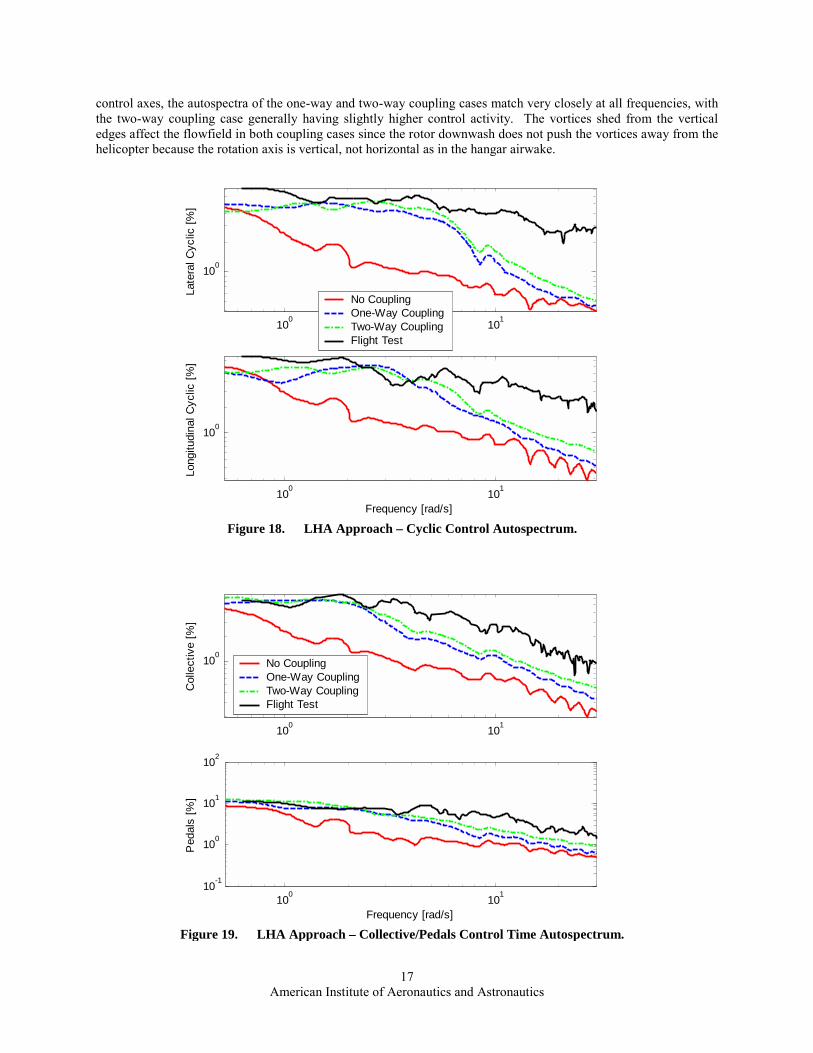
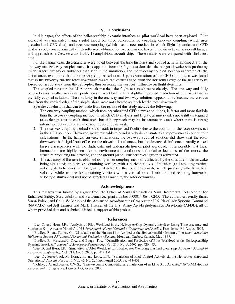
Figures 18 and 19 are autospectra of pilot (or pilot model) control activity obtained using CIFER®.26 As was

seen in the hangar runs, the no coupling case has the least activity for all control axes and the flight test generally has the most activity for the same reasons described earlier for the hangar airwake control autospectra. For all four

0 5 10 15 20 2520

30

40

50

60

70

Late

ral C

yclic

[%]

0 5 10 15 20 2520

40

60

80

100

Long

itudi

nal C

yclic

[%]

Time [s]


Figure 16. LHA Approach – Cyclic Control Time History.

0 5 10 15 20 25-20

0

20

40

60

80

Col

lect

ive

[%]

0 5 10 15 20 2520

40

60

80

100

Ped

als

[%]

Time [s]


Figure 17. LHA Approach – Collective/Pedals Control Time History.


17

control axes, the autospectra of the one-way and two-way coupling cases match very closely at all frequencies, with the two-way coupling case generally having slightly higher control activity. The vortices shed from the vertical edges affect the flowfield in both coupling cases since the rotor downwash does not push the vortices away from the helicopter because the rotation axis is vertical, not horizontal as in the hangar airwake.

100 101

100

Col

lect

ive

[%]

100 10110-1

100

101

102

Ped

als

[%]

Frequency [rad/s]


Figure 19. LHA Approach – Collective/Pedals Control Time Autospectrum.

100 101

100

Late

ral C

yclic

[%]

100 101

100

Long

itudi

nal C

yclic

[%]

Frequency [rad/s]


Figure 18. LHA Approach – Cyclic Control Autospectrum.


18

V. Conclusions In this paper, the effects of the helicopter/ship dynamic interface on pilot workload have been explored. Pilot

workload was simulated using a pilot model for three conditions: no coupling, one-way coupling (which uses precalculated CFD data), and two-way coupling (which uses a new method in which flight dynamics and CFD analysis codes run concurrently). Results were obtained for two scenarios: hover in the airwake of an aircraft hangar and approach to a Tarawa-class (LHA 1) amphibious assault ship. These results were compared with flight test data.

For the hangar case, discrepancies were noted between the time histories and control activity autospectra of the one-way and two-way coupled runs. It is apparent from the flight test data that the hangar airwake was producing much larger unsteady disturbances than seen in the simulation, and the two-way coupled solution underpredicts the disturbances even more than the one-way coupled solution. Upon examination of the CFD solutions, it was found that in the two-way run the rotor downwash causes the vortices shed from the horizontal edge of the hangar to be forced down and away from the helicopter, thus lessening the vortices’ influence on flight dynamics.

The coupled runs for the LHA approach matched the flight test much more closely. The one way and fully coupled cases resulted in similar predictions of workload, with a slightly improved prediction of pilot workload in the fully coupled solution. The similarity in the one-way and two-way solutions appears to be because the vortices shed from the vertical edge of the ship’s island were not affected as much by the rotor downwash.

Specific conclusions that can be made from the results of this study include the following: 1. The one-way coupling method, which uses precalculated CFD airwake solutions, is faster and more flexible

than the two-way coupling method, in which CFD analysis and flight dynamics codes are tightly integrated to exchange data at each time step, but this approach may be inaccurate in cases where there is strong interaction between the airwake and the rotor downwash.

2. The two-way coupling method should result in improved fidelity due to the addition of the rotor downwash in the CFD solution. However, we were unable to conclusively demonstrate this improvement in our current calculations. In the hangar airwake simulations, the two-way coupled solution did show that the rotor downwash had significant effect on the airwake disturbances, but the downwash influence actually caused larger discrepancies with the flight data and underprediction of pilot workload. It is possible that these interactions are highly sensitive to environmental conditions and relative locations of the rotors, the structure producing the airwake, and the ground plane. Further investigation is warranted.

3. The accuracy of the results obtained using either coupling method is affected by the structure of the airwake being simulated; an airwake containing vortices with a horizontal axis of rotation (and resulting vertical velocity disturbances) will be greatly affected by the rotor downwash, which primarily affects vertical velocity, while an airwake containing vortices with a vertical axis of rotation (and resulting horizontal velocity disturbances) will not be affected as much by the rotor downwash.

Acknowledgments This research was funded by a grant from the Office of Naval Research on Naval Rotorcraft Technologies for

Enhanced Safety, Survivability, and Performance, grant number N00014-06-1-0205. The authors especially thank Susan Polsky and Colin Wilkinson of the Advanced Aerodynamics Group at the U.S. Naval Air Systems Command (NAVAIR) and Jeff Lusardi and Mark Tischler of the U.S. Army Aeroflightdynamics Directorate (AFDD), all of whom provided data and technical advice in support of this project.

References 1Lee, D. and Horn, J.F., “Analysis of Pilot Workload in the Helicopter/Ship Dynamic Interface Using Time-Accurate and

Stochastic Ship Airwake Models,” AIAA Atmospheric Flight Mechanics Conference and Exhibit, Providence, RI, August 2004. 2Bradley, R. and Turner, G., “Simulation of the Human Pilot Applied at the Helicopter/Ship Dynamic Interface,” American

Helicopter Society 55th Annual Forum and Technology Display, Montreal, Quebec, Canada, May 1999. 3Bradley, R., Macdonald, C.A., and Buggy, T.A., “Quantification and Prediction of Pilot Workload in the Helicopter/Ship

Dynamic Interface,” Journal of Aerospace Engineering, Vol. 219, No. 5, 2005, pp. 429-443. 4Lee, D. and Horn, J.F., “Simulation of Pilot Workload for a Helicopter Operating in a Turbulent Ship Airwake,” Journal of

Aerospace Engineering, Vol. 219, No. 5, 2005, pp. 445-458. 5Lee, D., Sezer-Uzol, N., Horn, J.F., and Long, L.N., “Simulation of Pilot Control Activity during Helicopter Shipboard

Operations,” Journal of Aircraft, Vol. 42, No. 2, March-April 2005, pp. 448-461. 6Polsky, S.A, and Bruner, C.W.S., “Time-Accurate Computational Simulations of an LHA Ship Airwake,” 18th AIAA Applied

Aerodynamics Conference, Denver, CO, August 2000.


19

7Polsky, S.A., “A Computational Study of Unsteady Ship Airwake,” 40th AIAA Aerospace Sciences Meeting and Exhibit, Reno, NV, January 2002.

8Sezer-Uzol, N., Sharma, A., and Long, L.N., “Computational Fluid Dynamics Simulations of Ship Airwake,” Journal of Aerospace Engineering, Vol. 219, No. 5, 2005, pp. 369–392.

9Polsky, S. and Naylor, S., “CVN Airwake Modeling and Integration: Initial Steps in the Creation and Implementation of a Virtual Burble for F-18 Carrier Landing Simulations,” AIAA Modeling and Simulation Technologies Conference and Exhibit, San Francisco, CA, August, 2005.

10Woodson, S.H. and Ghee, T.A., “A Computational and Experimental Determination of the Air Flow Around the Landing Deck of a US Navy Destroyer (DDG),” 23rd AIAA Applied Aerodynamics Conference, Toronto, Ontario, Canada, June 2005.

11Polsky, S., Imber, R., Czerwiec, R., and Ghee, T., “A Computational and Experimental Determination of the Air Flow Around the Landing Deck of a US Navy Destroyer (DDG): Part II,” 37th AIAA Fluid Dynamics Conference and Exhibit, Miami, FL, June 2007.

12Lusardi, J.A., Tischler, M.B., Blanken, C.L., and Labows, S.J., “Empirically Derived Helicopter Response Model and Control System Requirements for Flight in Turbulence,” Journal of the American Helicopter Society, Vol. 49, No. 3, July 2004, pp. 340-349.

13Hess, R.A., “A Simplified Technique for Modeling Piloted Rotorcraft Operations Near Ships,” AIAA Atmospheric Flight Mechanics Conference and Exhibit, San Francisco, CA, August, 2005.

14Zan, S., “Experimental Determination of Rotor Thrust in a Ship Airwake,” Journal of the American Helicopter Society, Vol. 47, No. 2, April 2002, pp. 100-108.

15Lee, R.G. and Zan, S.J., “Wind Tunnel Testing of a Helicopter Fuselage and Rotor in a Ship Airwake,” 29th European Rotorcraft Forum, Friedrichshafen, Germany, Sept. 2003.

16Arunajatesan, S., Shipman, J.D., and Sinha, N., “Towards Numerical Modeling of Coupled VSTOL-Ship Airwake Flowfields,” 42nd AIAA Aerospace Sciences Meeting and Exhibit, Reno, NV, January 2004.

17Polsky, S.A. and Bruner, C.W., “Time Accurate CFD Analysis of Ship Air Wake with Coupled V-22 Flow,” Naval Air Warfare Center, Aircraft Division, Patuxent River, MD, 2000.

18Alpman, E., Long, L.N., Bridges, D.O., and Horn, J.F., “Fully Coupled Simulations of the Rotorcraft/Ship Dynamic Interface,” American Helicopter Society 63rd Annual Forum and Technology Display, Virginia Beach, VA, May 2007.

19Peters, D.A. and HaQuang, N., “Dynamic Inflow for Practical Applications,” Journal of the American Helicopter Society, Vol. 33, No. 4, October 1988, pp. 64-68.

20Alpman, E., Long, L.N., and Kothmann, B., “Understanding Ducted Rotor Antitorque and Directional Control Characteristics Part I: Steady Simulations,” Journal of Aircraft, Vol. 41, No. 5, September-October 2004, pp. 1042-1053.

21Alpman, E. Long, L.N., and Kothmann, B., “Understanding Ducted Rotor Antitorque and Directional Control Characteristics Part II: Unsteady Simulations,” Journal of Aircraft, Vol. 41, No. 6, November-December 2004, pp. 1370-1378.

22Howlett, J., “UH-60A BLACK HAWK Engineering Simulation Program: Volume I – Mathematical Model,” NASA CR-17742, USAAVSCOM TR 89-A-001, September 1989.

23Pacheco, P.S., “Parallel Programming with MPI,” Morgan Kaufmann Publishers, Inc., 1997. 24Costello, M., Gaonkar, G., Prasad, J., and Schrage, D., “Technical Notes: Some Issues on Modeling Atmospheric

Turbulence Experienced by Helicopter Rotor Blades,” Journal of the American Helicopter Society, Vol. 37, No. 2, April 1992, pp 71.

25Lusardi, J., “Control Equivalent Turbulence Input Model for the UH-60 Helicopter,” Special Report AMR-AF-06-01, August 2006.

26Tischler, M.B. and Cauffman, M.G., “Comprehensive Identification from Frequency Responses, Volume 1 – Class Notes,” NASA CP 10149, USAATCOM TR-94-A-017, 1994.

Coupled Flight Dynamics and CFD Analysis of Pilot Workload ... · Coupled Flight Dynamics and CFD...

Documents

Transcript of Coupled Flight Dynamics and CFD Analysis of Pilot Workload ... · Coupled Flight Dynamics and CFD...