1

Cost Inflexibility and Capital Structure*

QianQian Du Hong Kong University of Science and Technology

dqqmm@ust.hk

Laura Xiaolie Liu Hong Kong University of Science and Technology

and Cheung Kong Graduate School of Business Laura.xiaolei.liu@ust.hk

Rui Shen

Erasmus University rshen@rsm.nl

March 14, 2012

Abstract

We examine the empirical relationship between cost inflexibility and capital structure. We propose a cost inflexibility measure as a direct measure of a firm’s fixed cost proportion. We argue and show that this characteristic-based measure dominates previously used operating leverage measures because the sensitivity-based measure suffers from severe measurement error problems. We document that more cost inflexible firms are associated with lower debt ratio and shorter debt maturity. This single factor can explain about 16% to 23% of the cross-sectional variation in capital structure. One standard deviation increase of the inflexibility variable relates to 8% to 9% decrease of debt ratio. The association is stronger among financially constrained firms, value firms and firms with low profitability. Our evidence suggests that cost inflexibility is one of the most important determinants of capital structure in the cross-section.

*We thank Peter Mackay for helpful discussions. All errors are our own. We acknowledge the financial support from Hong Kong RGC (Project No: 643611).

2

I. Introduction

In a survey of CFOs, Graham and Harvey (2001) document “financial flexibility” to be

the most important determinant of a firm’s debt policy. Several recent papers model and analyze

the determinants of financial flexibility and its impacts on a firm’s investment and financing

policies.2 DeAngelo, DeAngelo and Whited (2011) model financial flexibility as unused debt

capacity and find it play an important role in a firm’s capital structure. Gamba and Triantis (2011)

characterize a financially flexible firm as one that is able to avoid financial distress during

recessions and fund investment during expansions. They find that among other variables, capital

inflexibility captures the irreversibility of investment, affects the value of financial flexibility and

is important in a firm’s financing decisions.

Capital inflexibility is commonly modeled in terms of capital adjustment costs and has

long been recognized to be an important risk driver.3 In fact, capital adjustment cost is only one

component of a firm’s cost structure. In this study we broaden the view of capital inflexibility to

incorporate other components of a firm’s cost structure to construct an aggregate cost

inflexibility measure. This was used to investigate its relationship with a firm’s financing policy.

Cost inflexibility captures not only the costly reversibility of capital investment, but also the fact

that a firm cannot painlessly cut its operating costs during economic downturns. If a firm’s

operating costs are entirely variable, when sales are high, costs are also high and when sales are

2 Denis and McKeon (2011) have documented how firms’ pro-active debt increases are consistent with the theory

that firms care about financial flexibility. Devos, Dhillon, Jagannathan and Krishnamurthy (2011) investigated first

debt initiation and found it to be consistent with a financial flexibility explanation. 3 See among others Berk, Green and Naik (1999), Gomes, Kogan and Zhang (2003), and Zhang (2005).

3

low, cost is also low. Variable costs can mitigate the effects of exogenous sales shocks so as to

maintain a relatively smooth earnings stream. On the other hand, if a firm’s operating costs are

mainly fixed, costs cannot be used as a hedge against sales shocks, so the firm’s earnings stream

is more correlated with the economic shocks. This makes firms with higher fixed costs more

vulnerable during economic downturns. Standard trade-off theory predicts that such firms should

have lower debt ratios.

Since the gap between revenues and costs is small for low profit firms, they suffer

disproportionately from any decrease in productivity which is not matched by a similar-sized

decrease in costs. Cost inflexibility will have a larger impact on such firms. Also, it is harder for

financially constrained firms to raise external funds to cover any financial deficit. This external

constraint magnifies the negative impact of fixed costs during bad times. This therefore suggests

that the negative relationship between cost inflexibility and leverage should be stronger for low

profit firms and for firms which are financially constrained.

Cost inflexibility is measured as selling, general and administration expense (SG&A

hereafter) divided by operating costs (SG&A plus the cost of goods sold). This measure differs

from most of the cost structure (or operating leverage) measures used in previously studies,

which have been based on estimated sensitivities. For example, Mandelker and Rhee (1984)

measured the sensitivity of profit to sales, while O’Brien and Vanderheiden (1987) and more

recently Kahl, Lunn and Nilsson (2011) measured the sensitivity of abnormal cost growth to

abnormal sales growth. Estimation errors in such regression analyses allow a characteristics-

based measure to provide a better, more accurate measure of cost inflexibility. And in this study

4

growth in the cost of goods sold (COGS hereafter) was indeed shown to have a stronger

covariance with sales growth than SG&A growth. The proposed inflexibility measure also does a

good job of capturing the degree by which a firm’s costs can serve as a hedge against variations

in the economic environment.

The main finding of this study is that the inflexibility variable by itself can explain about

16% of any cross-sectional variation in book leverage and 23% of that in market leverage. A one

standard deviation increase in inflexibility predicts an 8% decrease in book leverage and a 9%

decrease in market leverage. Compared to the existing capital structure determinants discussed

by Frank and Goyal (2009), the inflexibility variable promises to be one of the most important.

The results of this study also confirm that the effect of inflexibility on capital structure is

stronger in value firms, low-profit firms and financially constrained firms, as theory would

predict.

Finally, we show that our results are robust for incorporating more cost components and

for using different leverage measures and more importantly the cost inflexibility measure

strongly dominants other sensitive-based operating leverage measures in a horse race.

Our paper is most related to Kahl et. al.’s (2011) paper where they examine the relation

between operation leverage and capital structure. Our paper differs because we propose a

characteristics-based measure while they focus on the sensitivity-based measure. We argue and

provide supporting evidence that by avoiding measurement errors, the characteristics-based cost

structure measure significantly improves the ability to explain capital structure variation. Our

study is also related to MacKay (2003), who explore the relation between real flexibility and

5

capital structure. The real flexibility measure constructed in MacKay (2003) captures the

sensitivity of marginal production and investment decisions to variations in the economic

environment. With the advantage of being closely related to a theoretical model, the real

flexibility measure used in MacKay (2003) is relatively hard to construct and to apply in broader

samples. On the other hand, the measure we propose is very easy to construct and to use.

Our paper makes the following several contributions. First, we contribute to empirical

capital structure literature by documenting the importance of incorporating cost inflexibility in

debt ratio regressions. Second, we also contribute to the literature related to operation leverage.

Several recent asset pricing papers investigate the relationship between operating leverage and

asset return.4 We argue and show that directly measured fixed cost proportion is probably a

better measure of operating leverage than the sensitivity measure used in the exiting literature.

Finally, our paper contributes to the accounting cost stickiness literature. Managerial accounting

literature investigates the cross-sectional variation of cost-stickiness and the reasons behind it.5

We add to that literature by analyzing the impact of cost-stickiness on a firm’s financial policy.

The rest of the paper is organized as follows. Section 2 describes the data and our

inflexibility measure. Section 3 presents the argument and evidence that the inflexibility measure

dominates the existing sensitivity-based measure. Section 4 presents results of how the

inflexibility variable relates to capital structure. Section 5 provides all types of robustness checks

and Section 6 concludes.

4 See among others Gourio (2007), Novy-Marx (2011), and Favilukis and Lin (2011). 5 See among other Anderson, Banker and Janakiraman (2003) and Banker and Chen (2006).

6

II. Data and summary statistics

A. Sample

Our sample is Compustat annual data from 1971 to 2009. We start from 1971 since that is

when American firms started reporting cash flow statements. Following common practice, we

exclude financial firms (SIC code 6000-6999) and regulated utilities (SIC code 4900-4999), and

firms experiencing major mergers and acquisitions (Compustat sale_fn is “AB”). Also excluded

are firms with negative book value of equity, with missing book leverage, market leverage,

PP&E, EBIT, or Sales. We also require a firm to have at least 5 time-series observations. All

variables are deflated to constant 1983 dollars using Producer Price Index. Book leverage and

market leverage are trimmed to be between 0 and 1 and all the ratio variables are winsorized at

1st and 99th percentiles to remove the outliers. Detailed variable definitions can be found in

Appendix A. Our final sample has 144879 firm-year observations, representing 13622 unique

firms.6

B. Construction of cost inflexibility measure

We construct the cost inflexibility variable (InFlex hereafter) as SG&A, divided by the

summation of SG&A and COGS. By definition, COGS represents “all expenses that are directly

related to the cost of merchandise purchased or the cost of goods manufactured that are

withdrawn from finished goods inventory and sold to customers”, while SG&A represents “all

commercial expenses of operation (such as, expenses not directly related to product production)

6 If we restrict the sample to US firms only, the sample size becomes 128686 firm-year observations representing

11524 unique firms. The results are largely similar.

7

incurred in the regular course of business pertaining to the securing of operating income.” Since

COGS is directly related to product production, it is arguably more related to variable costs, a

point we will examine in more detail in the next subsection. InFlex thus proxies for the

proportion of fixed costs in a firm’s cost structure. We do not incorporate depreciation in the

InFlex calculation, because a firm’s depreciation may depend on the accounting rule a firm

chooses, which may not be related to a firm’s economic fundamentals. However, from another

perspective, depreciation is part of a firm’s cost structure. A capital-intensive firm uses more

tangible assets in its production process, resulting higher depreciation. Considering depreciation

of tangible assets as part of fixed costs, we construct InFlex2 by adding depreciation to both the

numerator and denominator.

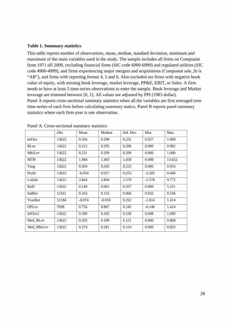
Table 1 reports the summary statistics of key variables used in this study. In panel A, we

report cross-sectional summary statistics by first taking the average of each variable across the

time-series of each firm to get one observation per firm. Panel B treats every firm-year as one

observation. On average, a firm has InFlex measure around 0.38 with median slightly lower than

the mean at 0.33. Book leverage has mean and median all around 0.3 and standard deviation of

0.21. Market leverage has a lower mean of 0.25 and median 0.21. The minimum leverage is 0

and maximum approaching 1. MTB measures market value of assets divided by book value of

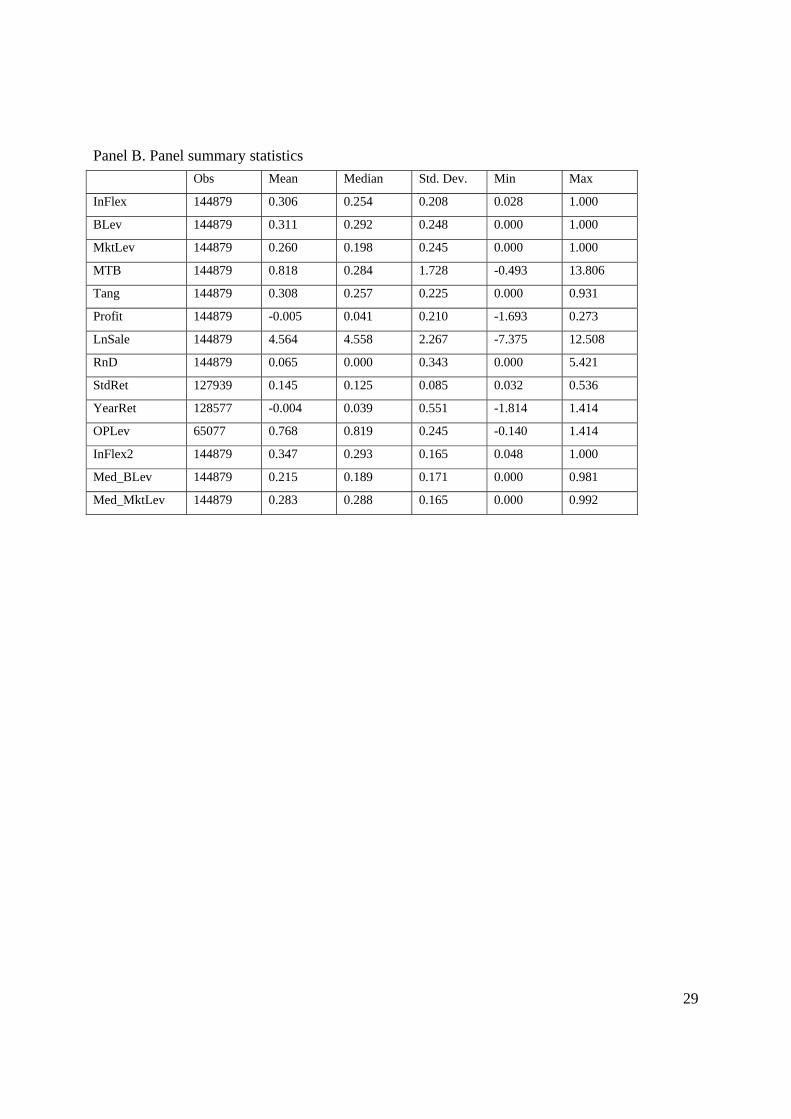
assets. The mean of MTB is 1.98 and median at 1.48. The summary statistics of panel sample are

largely comparable to those of the cross-sections.

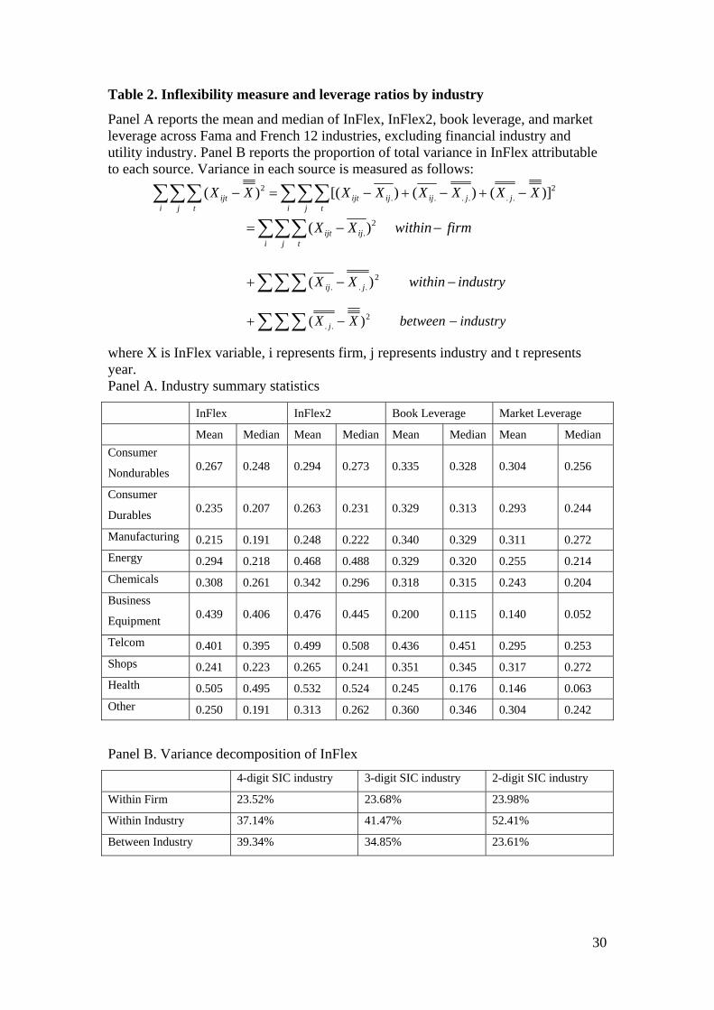
Panel A of Table 2 summarizes InFlex across 12 industries as classified by Fama-French,

but omitting the financial industry and utilities industry. The variable is highest in the health

8

industry (mean 0.51), business equipment industry (mean 0.44) and telecommunications industry

(mean 0.40) and lowest in manufacturing industry (mean 0.22), consumer durables industry

(mean 0.24), shops industry (mean 0.24) and consumer nondurables industry (mean 0.27). The

final product of the services industry is services rather than products, which require less raw

materials, but more man-power. Wage and R&D is probably the major input in the health

industry and telecommunications industry. On the other hand, manufacturing and consumer

goods industry deliver final products which require considerable variable costs such as raw

materials.

Adding depreciation increases the fixed cost proportion, yielding a higher value of

InFlex2. But the pattern across industries is in general similar to that of InFlex: high in health,

business equipment and telecommunications industries and low in manufacturing and consumer

goods industry. One industry that shows quite a different value of InFlex and InFlex2 is the

energy industry, which has medium InFlex value, but quite high InFlex2 value. The energy

industry needs significant amounts of tangible assets, resulting in a high level of depreciation. In

the robustness check section, we report our main results using InFlex2 and shows that the results

are similar with this alternative measure.

Also reported in Panel A of Table 2 is the mean and median of book and market leverage

ratio. Firms with high InFlex also shows somewhat low leverage ratio. For example, the health

and business equipment industries have book leverage as low as 0.25 and 0.20, and market

leverage 0.15 and 0.14; while manufacturing industry and consumer durables industry has book

leverage of 0.34 and 0.33 and market leverage 0.31 and 0.29. The table can serve as a simple

9

univariant test of the negative relation between InFlex and leverage ratio. However, we must

note the relation is not monotonic. This is partly due to the fact that we didn’t control for other

characteristics in the industry and also due to the fact that there are significant inter-industry

variations in both InFlex measure and leverage measure, which cannot be captured when we

average the measures in each industry.

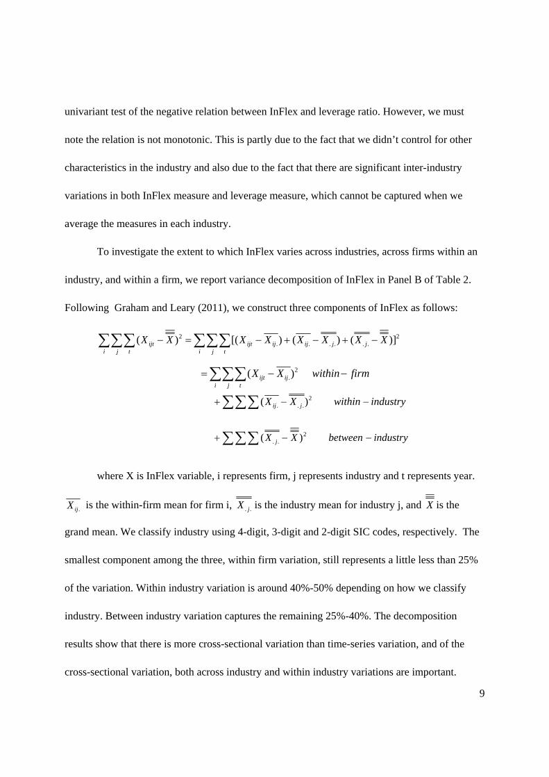
To investigate the extent to which InFlex varies across industries, across firms within an

industry, and within a firm, we report variance decomposition of InFlex in Panel B of Table 2.

Following Graham and Leary (2011), we construct three components of InFlex as follows:

i j t i j t

jjijijijtijt XXXXXXXX 2......

2 )]()()[()(

firmwithinXX

i j tijijt )( 2

.

industrywithinXX jij 　　2

... )(

industrybetweenXX j 　　2

.. )(

where X is InFlex variable, i represents firm, j represents industry and t represents year.

.ijX is the within-firm mean for firm i, .. jX is the industry mean for industry j, and X is the

grand mean. We classify industry using 4-digit, 3-digit and 2-digit SIC codes, respectively. The

smallest component among the three, within firm variation, still represents a little less than 25%

of the variation. Within industry variation is around 40%-50% depending on how we classify

industry. Between industry variation captures the remaining 25%-40%. The decomposition

results show that there is more cross-sectional variation than time-series variation, and of the

cross-sectional variation, both across industry and within industry variations are important.

10

These features are similar to that of leverage ratio as documented by many studies including

Lemmon, Robert and Zender (2008), MacKay and Phillips (2005) and Graham and Leary (2011),

although leverage ratio shows even higher within industry variation.

III. Flexibility measure

The relationship between a firm’s cost structure and it risk is quite intuitive. Variable

costs help firms smooth out dividend stream so that firm values do not covary much with

economic conditions. Fixed costs, on the other hand, do not have such a function. For firms with

a higher proportion of fixed costs in their costs structure, in response to negative shocks,

revenues fall more quickly than costs can be reduced, thus the profit (earning) is dampened more

in economic downturns.

Traditional interpretation of fixed cost focuses on usage of tangible assets as measured by

depreciation. Recent studies propose that wage expense is another form of fixed cost. Studies

such as Shimer (2005), Hall (2005), Gourio (2007), and Favilukis and Lin (2011) all argue that

wage is infrequently negotiated and sticky. It cannot be cut immediately and by a commensurate

amount when revenues are reduced. For firms where labor is an important input in their

production functions, earnings can be reduced more during bad times. R&D expense may also be

a form of fixed costs. Studies such as Li and Liu (2011) present evidence that intangible assets

are subject to much larger adjustment costs than tangible assets. If reflects that fact that it’s hard

to accumulate large intangible assets in a short period of time and it’s also hard to liquidate

intangible assets because the liquidation value is literally zero.

11

Based on simple trade-off theory, a firm with more fixed costs in its cost structure will

use less debt, resulting a lower leverage ratio.

Although theoretically compelling, the empirical support for the relationship between

cost inflexibility and capital structure is scarce.7 Part of the difficulty comes from the measure of

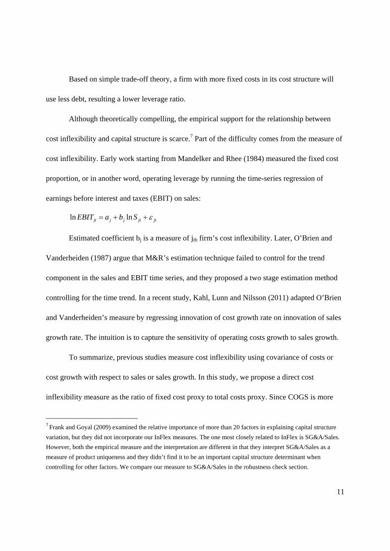
cost inflexibility. Early work starting from Mandelker and Rhee (1984) measured the fixed cost

proportion, or in another word, operating leverage by running the time-series regression of

earnings before interest and taxes (EBIT) on sales:

jtjtjjjt SbaEBIT lnln

Estimated coefficient bj is a measure of jth firm’s cost inflexibility. Later, O’Brien and

Vanderheiden (1987) argue that M&R’s estimation technique failed to control for the trend

component in the sales and EBIT time series, and they proposed a two stage estimation method

controlling for the time trend. In a recent study, Kahl, Lunn and Nilsson (2011) adapted O’Brien

and Vanderheiden’s measure by regressing innovation of cost growth rate on innovation of sales

growth rate. The intuition is to capture the sensitivity of operating costs growth to sales growth.

To summarize, previous studies measure cost inflexibility using covariance of costs or

cost growth with respect to sales or sales growth. In this study, we propose a direct cost

inflexibility measure as the ratio of fixed cost proxy to total costs proxy. Since COGS is more

7 Frank and Goyal (2009) examined the relative importance of more than 20 factors in explaining capital structure

variation, but they did not incorporate our InFlex measures. The one most closely related to InFlex is SG&A/Sales.

However, both the empirical measure and the interpretation are different in that they interpret SG&A/Sales as a

measure of product uniqueness and they didn’t find it to be an important capital structure determinant when

controlling for other factors. We compare our measure to SG&A/Sales in the robustness check section.

12

likely to be variable costs, we argue that other type of costs such as SG&A are mainly comprised

of fixed costs, relatively speaking. Thus, the ratio of SG&A to the sum of COGS and SG&A

provides a simplified measure of fixed cost proportion in a firm’s cost structure, thus serving as a

proxy of cost inflexibility.

We prefer this characteristic-based measure to the previously used sensitivity measure for

two reasons. First of all, InFlex is easy to construct. It is available for all firm years no matter

how many time series observations a firm has and whether a firm has positive or negative EBIT.

More importantly, compared with the sensitivity-based measures, InFlex suffers fewer

measurement error problems. It has long been recognized that covariance measures may have

significant measurement errors (see for example, Miller and Scholes (1972), Whited (1994)). A

recent study by Lin and Zhang (2011) carefully examined the measurement error problem in

covariance estimation. Although they focused on the asset pricing application of covariance

measure, the spirit of the argument applies to the sensitivity measure of operating leverage as

well. In a later section, we compare our measure with the previously used sensitivity measure

and show that the explanatory power of InFlex is an order of magnitude higher than that of the

sensitivity measure.

To verify this measure, we implement several tests. If COGS is mainly variable costs, it

should closely co-move with sales. We first test this hypothesis using aggregate level data. For

each year, we aggregate all the sales, COGS and SG&A for firms with December fiscal year end

into aggregate level variables. We restrict the analyses to firms with December fiscal year end to

make sure that the aggregations cover the same time period. Based on these aggregate variables,

13

we calculate the natural logarithm of growth rate. Figure 1 presents the growth rate of these three

series. Several features of the graphs are worth noting. First, sales growth varies over time, being

high in certain years such as 1999-2000 and 2008, and low in some other years including 2009,

1982 and 1975. Second and most importantly, COGS growth rate is closely aligned with sales

growth rate. In most years, these two series overlap with each other. In several years when they

separate, the gap between them is very small. This becomes more obvious when comparing with

the time series of SG&A. Third, the variation of SG&A is much smaller than that of Sale and

COGS series. SG&A series trends up more slowly and falls down more slowly. This feature of

SG&A is consistent with the argument that SG&A can be treated as a proxy for fixed costs.

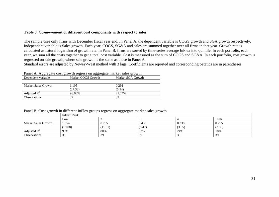
We then formally test the co-movement of different cost components with respect to

aggregate sales growth rate using regressions. Table 3 reports the regression results. Panel A

reports results using aggregate data while panel B reports results using portfolio level data. From

1971 to 2009, the aggregate level data comprises 39 observations. Standard errors are Newey-

West adjusted for three lags. When the dependent variable is logarithm growth rate of COGS, the

coefficient is close to 1 (1.11), with R2 as high as 0.97. With SG&A growth rate as the dependent

variable, the coefficient is only 0.29 with R2 0.21. The results strongly support the argument that

COGS moves more closely with sales, thus is more likely to represent variable costs while

SG&A is more related to fixed costs. Since COGS moves closely with sales, it serves as a hedge,

reducing the co-movement of gross profits with sales; while SG&A is rather independent of sales

movement, the difference between sales and SG&A still has high co-movement with total sales.

Consistent with this, unreported results shows that used as dependent variable, the growth rate of

14

gross profit has coefficient of 0.80 with R2 0.76 while the growth rate of sales minus SG&A has

coefficient of 1.14 with R2 0.99.

Next, we replicate the regressions using portfolio level data. We first take average of

InFlex over the time series of each firm to get one value per firm. As in Panel A, we restrict the

sample to firms with December fiscal year end. We sort firms using this averaged InFlex

measure into quintiles. Low group has the smallest value of InFlex, representing the smallest

fixed cost proportion in firms’ cost structure, while high group implies high fixed cost proportion.

In each portfolio, we sum COGS and SG&A to obtain portfolio level data series. We then add up

COGS and SG&A to get total costs series and calculate logarithm growth rate of total costs for

each portfolio. We next regress portfolio-level operating cost growth on market level sales

growth. The coefficients show a monotonic decreasing pattern, from 1.35 for low InFlex quintile

to 0.30 for high InFlex quintile. A similar decreasing pattern shows up in R2, from 0.90 down to

0.18. The decreasing patterns of coefficient and R2 are consistent with the argument that InFlex

captures the riskiness reflected in a firm’s cost structure. Firms with high InFlex has higher risk

because their costs are less of a hedge for the variation of economic growth.

In this section, we present argument and evidence that InFlex can be used as a proxy of

fixed cost proportions, which positively relates to the risk faced by a firm. We next formally

examine the relation between InFlex and capital structure.

15

IV. Empirical results

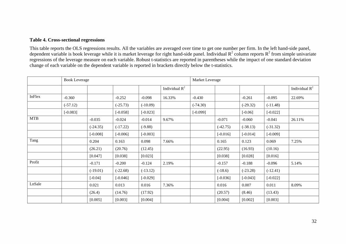
Since both InFlex and leverage ratio have more cross-sectional variations, we start from

analyzing the cross-sectional explanatory power of InFlex on capital structure. Table 4 reports

cross-sectional regression results of leverage on InFlex and other control variables. This is the

main result of this study. Used as a sole regressor, InFlex has coefficient of -0.36, which is

highly significant and R2 is 16.33%. The second column reports regression with commonly used

explanatory variables: market-to-book asset ratio, tangibility ratio, profitability, firm size

measured by natural log of sales and R&D expenditure over sales. Market-to-book asset ratio,

profitability and R&D ratio have negative coefficients, while tangibility and Ln(sales) have

positive coefficients. These results are consistent with those documented in previous studies. All

these variables adding together have R2 about 19%, only slightly higher than the R2 of InFlex by

itself. After controlling all these variables, InFlex is still highly significant with coefficient -0.25.

Adding InFlex increases R2 by about a quintile. In the fourth column, we add more control

variables including standard deviation of monthly stock return in previous year, cumulative stock

return in previous year and median book leverage in the same industry measured by 4-digit SIC

code, all of which are suggested to be important variables by Frank and Goyal (2009). Adding

industrial median leverage significantly increases explanatory power, as documented in other

studies. The last column of this panel reports R2 from simple univariate regressions of the

leverage measure on each variable. Industry median leverage has the highest individual R2,

34.6%, followed by InFlex, 16.3%, followed by MTB with R2 9.67%, and then by Tangibility

and Ln(Sale) with R2 around 7%. InFlex has individual R2 almost double that of all other

16

variables, except for industry median leverage ratio. The results for market leverage regression

are largely similar. By itself, InFlex explains 23% of debt ratio variation. Adding other control

variables doesn’t change its explanatory power.

Reported in brackets are economic significances which represent the percentage change

of leverage ratio corresponding to one standard deviation change of each independent variable.

Individually, one standard deviation increase of InFlex is related to an 8% decrease of book

leverage ratio and a 9% decrease of market leverage ratio. These numbers suggest that InFlex is

not only statistically but also economically important. The economic significance is also larger

than most of the other variables, except for industry median leverage ratio. Although generating

the highest R2 and economic significance, industry median leverage only captures industry effect

and doesn’t answer the question of why leverage ratio exhibits industry effects. To address that

issue, we still need to search for firm-specific characteristics variables such as InFlex.

Panel regressions results are largely similar and are reported in Table 5. InFlex is

negatively related to both book leverage and market leverage, although the individual R2 values

are much smaller than those obtained in cross-sectional regression, 6.61% for book leverage and

11.29% for market leverage.

So far, we have shown that InFlex is important in explaining capital structure variation

because it captures a firm’s cost structure, and is thus related to a firm’s risk. Based on this

argument, the effect of InFlex should be stronger for low productivity firms. Firms with low

productivity have higher risk because the gap between revenues and costs is small. They suffer

disproportionately from a decrease in productivity which is not matched by a similar-sized

17

decrease in costs. Also they are the firms most likely to experience negative profits, thus being

unable to service debt during recessions. For similar reason, the effect of InFlex on leverage

should also be stronger for financially constrained firms. It is harder for financially constrained

firms to raise external funds when needed to cover their financial deficit, thus the negative

impacts of costs can be more severe for financially constrained firms.

We measure low productivity using profit and market-to-book ratio. It has long been

shown that value firms have low profit, thus, the effects of InFlex should be stronger in value

firms. It should also be stronger in low profit firms, as measured by profit before extraordinary

items divided by assets. We measure financial constraints in two ways: whether a firm has paid

dividend in previous year, and whether the firm has credit rating in previous year. We add an

interaction term of InFlex with dividend dummy, taking a value of 1 if a firm has ever payed

dividend and 0 otherwise; also rating dummy taking a value of 1 if a firm has credit rating and 0

otherwise.

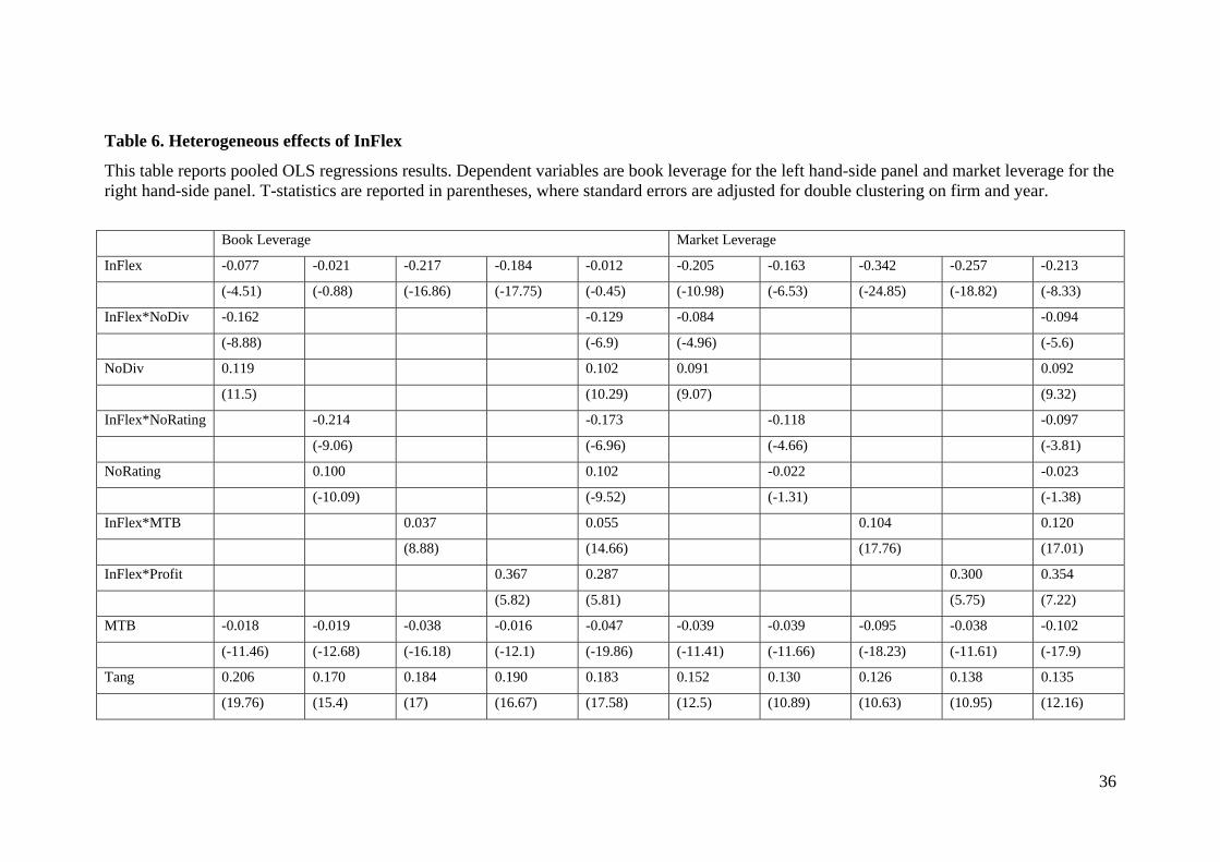
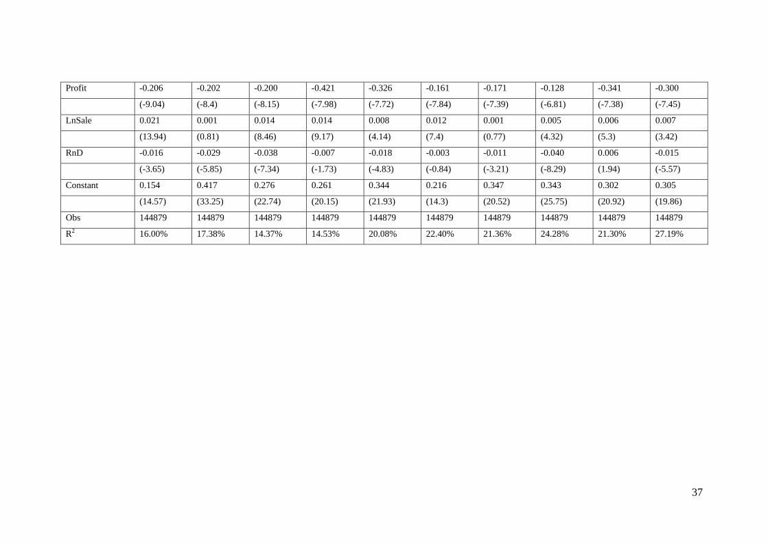
Table 6 presents the results of this analysis. As we expected, the explanatory power of

InFlex is much stronger in financially constrained firms. Compared to dividend paying firms, the

coefficient of InFlex for non-dividend paying firms is 0.162 lower. The difference is statistically

significant. The firms without rating have coefficient -0.23 (-0.02 + -0.21) while firms with

rating have coefficient -0.02 only. There is strong evidence that the effect of InFlex is

concentrated in financially constrained firms.

For firms with high profitability, the effect of InFlex is smaller with InFlex*Profitability

having a positive and significant coefficient. Similarly, the effect of InFlex is smaller in growth

18

firms with InFlex*MTB having positive coefficient although the effect is much smaller than

measuring using profitability directly. This is partly due to the fact that MTB is an indirect

measure of productivity.

The right-hand panel of Table 5 reports market leverage regression. All of the results

hold in market leverage as well.

V. Robustness Check

In this section, we provide various robustness tests for our results.

A. Alternative InFlex measures

The InFlex measure we used in previous tests does not consider depreciation, while

InFlex2 does.

Panel A and B of Table 7 report cross-sectional and panel regression results using

InFlex2 as the key explanatory variable. In cross-sectional regressions, InFlex2 has coefficient -

0.246 in book leverage regression and -0.266 in market leverage regression. Both are highly

significant. The coefficients of all control variables have the same signs and similar magnitude.

Panel regressions show similar results. Adding depreciation into the measure doesn’t change the

results, qualitatively or quantitatively. Unreported tables show that if we defined total cost as

sales minus income before extraordinary items excluding interest expense, instead of sum of

SG&A and COGS, tenure of the results does not change.

19

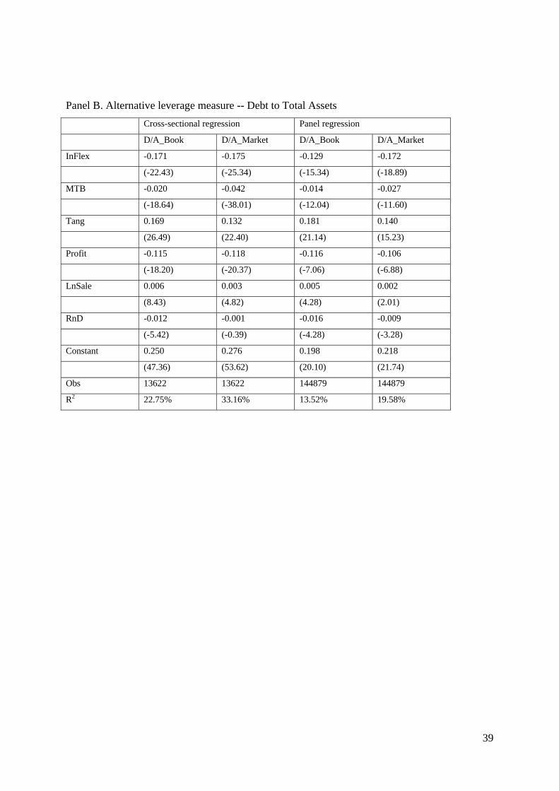
B. Alternative leverage measures

We define leverage as debt divided by the sum of equity and debt. This measure excludes

financial liability, which is the measure proposed by Welch (2011). As a robustness check, we

also construct traditional leverage measures as debt divided by total book or market assets. The

results based on these measures are reported in Panel B of Table 8. Again, the results are largely

similar.

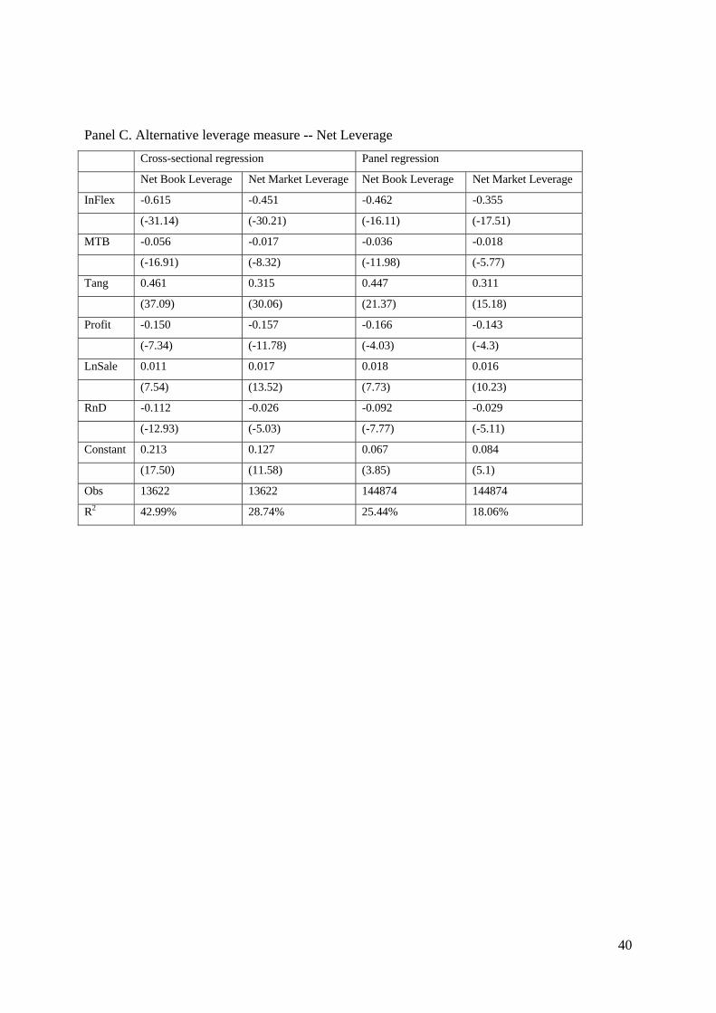
Bates, Kahle and Stulz (2009) reported that cash holding of US firms is increasing over

time and in recent years, the total cash holdings are larger than total debt holdings, resulting in

negative net debt holding. However, studies such as Acharya, Almeida and Campello (2007)

argued that cash should not be viewed as negative debt in the presence of financing frictions.

Studying the cash policy by itself is an interesting topic, but it goes beyond the scope of this

study. Nevertheless, we construct a net leverage ratio measure by taking out cash from the

numerator to make sure that the results are not purely driven by the cash component. Estimation

results using net leverage ratio as dependent variables are reported in Table 8 Panel C. The

coefficient of InFlex becomes much larger, -0.62 in book leverage and -0.45 in market leverage

regressions. The R2 is also much higher although it is not appropriate to compare R2 of this table

with those reported in other tables since the dependent variables are different. The results suggest

that our previous documented negative relation between InFlex and leverage is not purely driven

by the cash component.

20

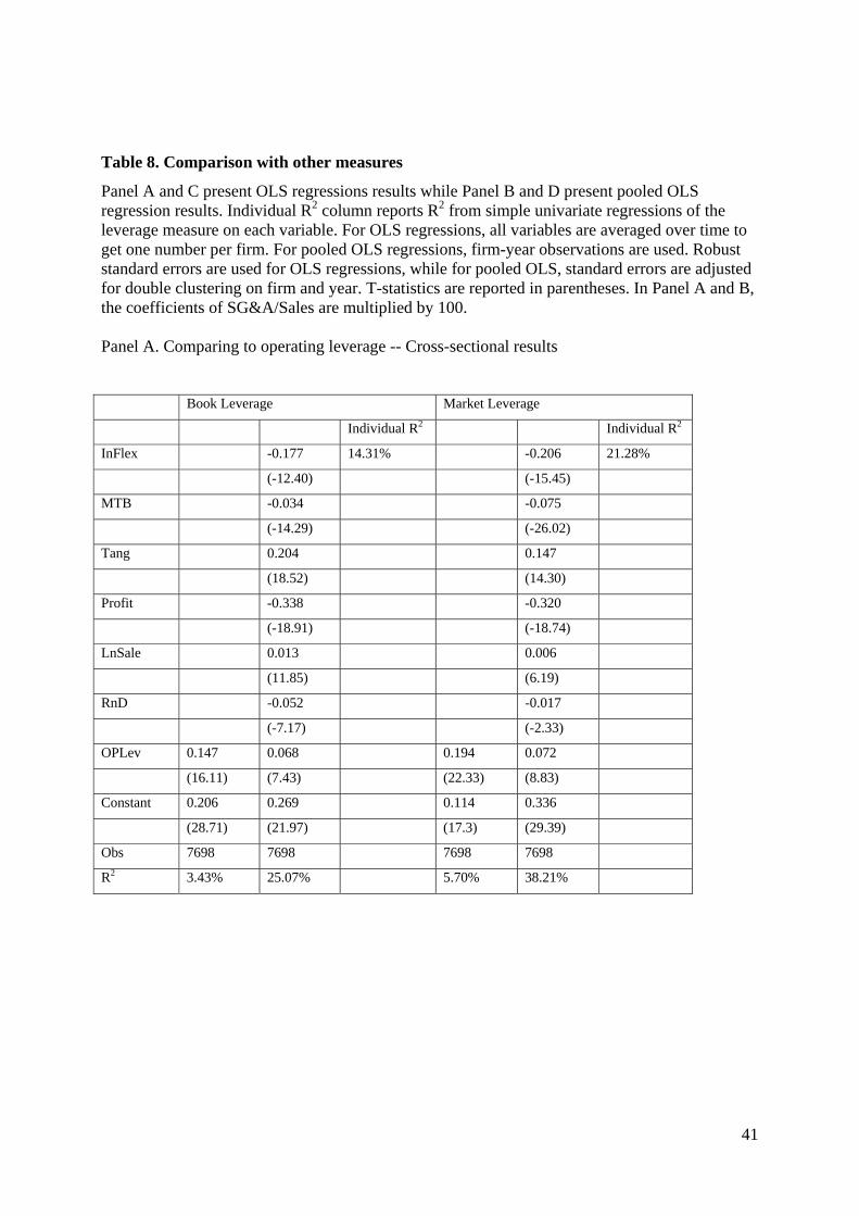
C. Comparing with other measures

Finally, we compare our measure with the operating leverage measure used in Kahl et al.

(2011) and SG&A ratio measure reported in Frank and Goyal (2009). Kahl et al. measure

operating leverage as the coefficient in the following regression:

,)()(

,1,

,,,

1,

,,tj

tj

tjtjtj

tj

tjtj

S

SESb

C

CEC

where

2/1

3,

1,1,, ][

tj

tjtjtj S

SSSE , and

2/1

3,

1,1,, ][

tj

tjtjtj C

CCCE

S represents sales and C represents the summation of COGS and SG&A. The regression

is estimated using the past seven years’ data as in Kahl et al. The availability of data reduces the

sample size from 13622 to 7698 unique firms. In this overlapping sample, OpLev by itself

generate R2 of 3.43% in book leverage regressions and 5.70% in market leverage regressions;

while comparable R2 for InFlex is 14.31% and 21.28%. Comparing using R2, InFlex has

explanatory power an order of magnitude higher than OpLev. Similar results obtain in panel

regressions. As previously argued, InFlex can obtain higher explanatory power at least in part

because it suffers less from the measurement errors problem in other sensitivity measures such as

OpLev.

Kayhan and Titman (2007) include SG&A/Sales as a control variable, arguing that it

measures the uniqueness of the firm’s products and the uniqueness of the firm’s collateral. Frank

and Goyal (2009) incorporate SG&A/Sales in their list of explanatory variables, but they do not

find it to be an important determinant after controlling other variables. The results of InFlex

comparing with SG&A/Sales are reported in Panel C and D of Table 8. We multiply the

coefficient of SG&A/Sales by 100 to make it readable. We confirmed the results documented in

Frank and Goyal (2009), the individual R2 of SG&A/Sales is always less than 1% and the

coefficient is minimum. The explanatory power of InFlex doesn’t change with the presence of

SG&A/Sale. It seems likely that SG&A/Sales, used as a product uniqueness measure, does not

capture the similar fundamental as InFlex.

21

VI. Conclusion

Traditional trade-off theory predicts that firms with less flexibility in terms of high fixed

cost in their cost structure should have lower leverage. Higher fixed costs are harder to cut

during economic downturns, resulting in a lower after cost profit, which increases a firm’s

bankruptcy costs. Ceteris paribus, a firm with higher fixed costs in their cost structure should

borrow less debt.

In this study, we propose a cost inflexibility measure (InFlex) as a direct measure of the

proportion of fixed cost of a firm’s operating cost. We consider two main components in a firm’s

total cost, COGS and SG&A. We use SG&A as a proxy for fixed cost and COGS as variable cost.

We argue that our measure is preferable to the previously used sensitivity measure because it is

less likely to suffer from measurement errors problem. We verify our measure by showing that at

aggregate level, total COGS growth more closely relates to sales growth than SG&A growth.

Next, when we sort firms by InFlex into five groups, we show that the coefficients of cost

growth on sales growth are monotonically decreasing from low InFlex group to high InFlex

group.

In the main tests, we show that in cross-sectional regression, InFlex by itself can explain

about 16% of book leverage variation and 23% of market leverage variation. With other control

variables, InFlex can increase the explanatory power by about one fifth. We further show that the

results are stronger in value firms, in low profit firms and in financially constrained firms,

measured by non-dividend paying firms, or firms without credit rating. Value firms, low profit

firms and financially constrained firms may suffer more during economic downturns, thus the

22

difficulty in cutting costs during bad times becomes especially challenging for these firms. Our

results are consistent with this hypothesis.

We further show that our results are robust when compared with different measures of

leverage and several alternative measures of costs considering more components. Last but not

least, we show that InFlex perform much better than previously used sensitivity-based cost

structure measures in a horse race.

To conclude, we argue that it is important to consider cost inflexibility in explaining a

firm’s cross-sectional capital structure and we show that a simple measure of fixed cost

proportion performs much better than the traditionally used sensitivity-based measure, probably

due to the measure errors problems in the latter.

23

Reference:

Acharya, V., H. Almeida and M. Campello, 2007. Is cash negative debt? A hedging perspective

on corporate financial policies. Journal of Financial Intermediation 16, 515-554.

Anderson, M., R. Banker and S. Janakiraman, 2003. Are Selling, General, and Administrative

Costs “Sticky”? Journal of Accounting Research 41, 47-63.

Banker, R. and L. Chen, 2006. Predicting Earnings Using a Model Based on Cost Variability and

Cost Stickiness. The Accounting Review 81, 285-307.

Berk, Jonathan B., Richard C. Green, and Vasant Naik, 1999, Optimal investment, growth

options and security returns, Journal of Finance, 54, 1153–1607.

DeAngelo, H., DeAngelo, L., Whited, T., 2011. Capital structure dynamics and transitory debt.

Journal of Financial Economics 99, 235-261.

Denis, David and Steve McKeon, Debt Financing and Financial Flexibility: Evidence from Pro-

Active Leverage Increases, 2011, Review of Financial Studies, forthcoming.

Devos, Erik, Upinder Dhillon, Murali Jagannathan and Srinivasan Krishnamurthy, 2011, Why

are Firms Unlevered? A Comparison of the Managerial Entrenchment, Tax, and Financial

Flexibility Hypotheses , working paper.

Frank, Murray Z., and Vidhan K. Goyal, 2009, Capital Structure Decisions: Which Factors Are

Reliably Important? Financial Management 38, 1-37.

Favilukis, J. and X. Lin, 2011. Micro Frictions, Asset Pricing, and Aggregate Implications.

Working paper, London School of Economics & Political Science and Ohio State

University.

24

Gamba, A. and A.J. Triantis, “The Value of Financial Flexibility” Journal of Finance, Vol. 63,

No. 5 (October 2008), 2263-2296.

Gomes, Joao F., Leonid Kogan, and Lu Zhang, 2003, Equilibrium cross section of returns,

Journal of Political Economy, 111, 693–732.

Gourio, F., 2007. Labor Leverage, Firms.Heterogeneous Sensitivities to the Business Cycle, and

the Cross-Section of Expected Returns. Working paper, Boston University and NBER.

Graham, John R., and Campbell Harvey, 2001, The Theory and Practice of Corporate Finance:

Evidence from the Field, Journal of Financial Economics 60, 187-243

Graham, J. and M. Leary, 2011. A Review of Empirical Capital Structure Research and

Directions for the Future. Annual Review of Financial Economics 3, 309-345.

Hall, Robert, 2005, Employment Fluctuations with Equilibrium Wage Stickiness, American

Economic Review 95 (1), 50-65.

Kahl, Matthias, Jason Lunn, and Mattias Nilsson, Operating Leverage and Corporate Financial

Policies, 2011, working paper.

Lemmon, M., M. Roberts and J. Zender, 2008. Back to the Beginning: Persistence and the Cross-

Section of Corporate Capital Structure. The Journal of Finance 63, 1575–1608.

Li, Erica Xuenan and Laura Xiaolei Liu, 2011, Intangible Assets and Stock Returns: Evidence

from The Structural Estimation, Cheung Kong Graduate School of Business and Hong

Kong University of Science and Technology, Working paper.

Lin, Xiaoji and Lu Zhang, 2011, Covariance, Characteristics, and General Equilibrium: A

Critique, Ohio State University, Working paper.

25

MacKay, P., 2003. Real Flexibility and Financial Structure: An Empirical Analysis. Review of

Financial Studies 16, 1131-1165.

MacKay, P. and G. Phillips, 2005. How Does Industry Affect Firm Financial Structure? Review

of Financial Studies 18, 1433-1466.

Mandelker, Gershon N., and S. Ghon Rhee, 1984, The Impact of the Degrees of Operating and

Financial Leverage on Systematic Risk of Common Stock, Journal of Financial and

Quantitative Analysis, 19, 45-57.

Miller, M. and M. Scholes, 1972. Rates of return in relation to risk: A reexamination of some

recent findings. Studies in the Theory of Capital Markets, New York: Praeger.

Novy-Marx, R., 2011. Operating Leverage. Review of Finance 15, 103-134.

O’Brien T., and P. Vanderheiden, 1987. Empirical Measurement of Operating Leverage for

Growing Firms. Financial Management 16, 45-53.

Shimer, Robert, 2005, The Assignment of Workers to Jobs in an Economy with Coordination

Frictions, Journal of Policital Economy,

Welch, I., 2011. Two Common Problems in Capital Structure Research: The Financial-Debt-To-

Asset Ratio and Issuing Activity Versus Leverage Changes. International Review of

Finance 11, 1-17.

Whited, T., 1994. Problems with Identifying Adjustment Costs From Regressions of Investment

on q. Economics Letters 46, 327-332.

Zhang, Lu, 2005, The Value Premium, Journal of Finance, February 2005, 67-103.

26

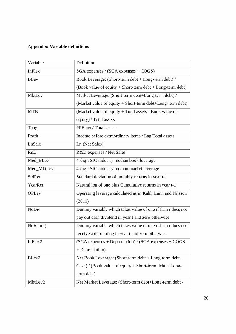
Appendix: Variable definitions

Variable Definition

InFlex SGA expenses / (SGA expenses + COGS)

BLev Book Leverage: (Short-term debt + Long-term debt) /

(Book value of equity + Short-term debt + Long-term debt)

MktLev Market Leverage: (Short-term debt+Long-term debt) /

(Market value of equity + Short-term debt+Long-term debt)

MTB (Market value of equity + Total assets - Book value of

equity) / Total assets

Tang PPE net / Total assets

Profit Income before extraordinary items / Lag Total assets

LnSale Ln (Net Sales)

RnD R&D expenses / Net Sales

Med_BLev 4-digit SIC industry median book leverage

Med_MktLev 4-digit SIC industry median market leverage

StdRet Standard deviation of monthly returns in year t-1

YearRet Natural log of one plus Cumulative returns in year t-1

OPLev Operating leverage calculated as in Kahl, Lunn and Nilsson

(2011)

NoDiv Dummy variable which takes value of one if firm i does not

pay out cash dividend in year t and zero otherwise

NoRating Dummy variable which takes value of one if firm i does not

receive a debt rating in year t and zero otherwise

InFlex2 (SGA expenses + Depreciation) / (SGA expenses + COGS

+ Depreciation)

BLev2 Net Book Leverage: (Short-term debt + Long-term debt -

Cash) / (Book value of equity + Short-term debt + Long-

term debt)

MktLev2 Net Market Leverage: (Short-term debt+Long-term debt -

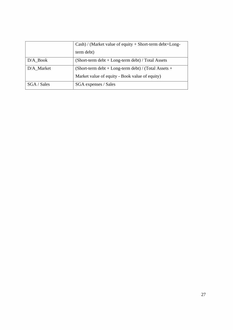
27

Cash) / (Market value of equity + Short-term debt+Long-

term debt)

D/A_Book (Short-term debt + Long-term debt) / Total Assets

D/A_Market (Short-term debt + Long-term debt) / (Total Assets +

Market value of equity - Book value of equity)

SGA / Sales SGA expenses / Sales

28

Table 1. Summary statistics

This table reports number of observations, mean, median, standard deviation, minimum and maximum of the main variables used in the study. The sample includes all firms on Compustat from 1971 till 2009, excluding financial firms (SIC code 6000-6999) and regulated utilities (SIC code 4900-4999), and firms experiencing major mergers and acquisitions (Compustat sale_fn is “AB”), and firms with reporting format 4, 5 and 6. Also excluded are firms with negative book value of equity, with missing book leverage, market leverage, PP&E, EBIT, or Sales. A firm needs to have at least 5 time-series observations to enter the sample. Book leverage and Market leverage are trimmed between [0, 1]. All values are adjusted by PPI (1983 dollar). Panel A reports cross-sectional summary statistics when all the variables are first averaged over time-series of each firm before calculating summary statics. Panel B reports panel summary statistics where each firm-year is one observation.

Panel A. Cross-sectional summary statistics

Obs Mean Median Std. Dev. Min Max

InFlex 13622 0.356 0.298 0.231 0.027 1.000

BLev 13622 0.312 0.295 0.206 0.000 0.982

MktLev 13622 0.251 0.209 0.209 0.000 1.000

MTB 13622 1.984 1.483 1.459 0.498 13.652

Tang 13622 0.304 0.243 0.223 0.000 0.933

Profit 13622 -0.054 0.027 0.253 -2.205 0.440

LnSale 13622 3.844 3.894 2.279 -2.578 9.772

RnD 13622 0.149 0.001 0.557 0.000 5.251

StdRet 12161 0.163 0.152 0.066 0.032 0.536

YearRet 12184 -0.074 -0.016 0.262 -1.814 1.414

OPLev 7698 0.756 0.807 0.245 -0.140 1.414

InFlex2 13622 0.399 0.345 0.230 0.048 1.000

Med_BLev 13622 0.205 0.189 0.151 0.000 0.868

Med_MktLev 13622 0.274 0.281 0.154 0.000 0.823

29

Panel B. Panel summary statistics

Obs Mean Median Std. Dev. Min Max

InFlex 144879 0.306 0.254 0.208 0.028 1.000

BLev 144879 0.311 0.292 0.248 0.000 1.000

MktLev 144879 0.260 0.198 0.245 0.000 1.000

MTB 144879 0.818 0.284 1.728 -0.493 13.806

Tang 144879 0.308 0.257 0.225 0.000 0.931

Profit 144879 -0.005 0.041 0.210 -1.693 0.273

LnSale 144879 4.564 4.558 2.267 -7.375 12.508

RnD 144879 0.065 0.000 0.343 0.000 5.421

StdRet 127939 0.145 0.125 0.085 0.032 0.536

YearRet 128577 -0.004 0.039 0.551 -1.814 1.414

OPLev 65077 0.768 0.819 0.245 -0.140 1.414

InFlex2 144879 0.347 0.293 0.165 0.048 1.000

Med_BLev 144879 0.215 0.189 0.171 0.000 0.981

Med_MktLev 144879 0.283 0.288 0.165 0.000 0.992

30

Table 2. Inflexibility measure and leverage ratios by industry

Panel A reports the mean and median of InFlex, InFlex2, book leverage, and market leverage across Fama and French 12 industries, excluding financial industry and utility industry. Panel B reports the proportion of total variance in InFlex attributable to each source. Variance in each source is measured as follows:

i j t i j t

jjijijijtijt XXXXXXXX 2......

2 )]()()[()(

firmwithinXX

i j tijijt )( 2

.

industrywithinXX jij 　　2... )(

industrybetweenXX j 　　2

.. )(

where X is InFlex variable, i represents firm, j represents industry and t represents year. Panel A. Industry summary statistics

InFlex InFlex2 Book Leverage Market Leverage

Mean Median Mean Median Mean Median Mean Median

Consumer

Nondurables 0.267 0.248 0.294 0.273 0.335 0.328 0.304 0.256

Consumer

Durables 0.235 0.207 0.263 0.231 0.329 0.313 0.293 0.244

Manufacturing 0.215 0.191 0.248 0.222 0.340 0.329 0.311 0.272

Energy 0.294 0.218 0.468 0.488 0.329 0.320 0.255 0.214

Chemicals 0.308 0.261 0.342 0.296 0.318 0.315 0.243 0.204

Business

Equipment 0.439 0.406 0.476 0.445 0.200 0.115 0.140 0.052

Telcom 0.401 0.395 0.499 0.508 0.436 0.451 0.295 0.253

Shops 0.241 0.223 0.265 0.241 0.351 0.345 0.317 0.272

Health 0.505 0.495 0.532 0.524 0.245 0.176 0.146 0.063

Other 0.250 0.191 0.313 0.262 0.360 0.346 0.304 0.242

Panel B. Variance decomposition of InFlex

4-digit SIC industry 3-digit SIC industry 2-digit SIC industry

Within Firm 23.52% 23.68% 23.98%

Within Industry 37.14% 41.47% 52.41%

Between Industry 39.34% 34.85% 23.61%

31

Table 3. Co-movement of different cost components with respect to sales The sample uses only firms with December fiscal year end. In Panel A, the dependent variable is COGS growth and SGA growth respectively. Independent variable is Sales growth. Each year, COGS, SG&A and sales are summed together over all firms in that year. Growth rate is calculated as natural logarithm of growth rate. In Panel B, firms are sorted by time-series average InFlex into quintile. In each portfolio, each year, we sum all the costs together to get a total cost variable. Cost is measured as the sum of COGS and SG&A. In each portfolio, cost growth is regressed on sale growth, where sale growth is the same as those in Panel A. Standard errors are adjusted by Newey-West method with 3 lags. Coefficients are reported and corresponding t-statics are in parentheses. Panel A. Aggregate cost growth regress on aggregate market sales growth Dependent variable Market COGS Growth Market SGA Growth Market Sales Growth 1.105

(27.33) 0.291 (5.54)

Adjusted R2 96.66% 21.24% Observations 39 39 Panel B. Cost growth in different InFlex groups regress on aggregate market sales growth InFlex Rank Low 2 3 4 High Market Sales Growth 1.354 0.735 0.430 0.338 0.295 (19.88) (11.31) (6.47) (3.65) (3.30) Adjusted R2 90% 80% 32% 24% 18% Observations 39 39 39 39 39

32

Table 4. Cross-sectional regressions

This table reports the OLS regressions results. All the variables are averaged over time to get one number per firm. In the left hand-side panel, dependent variable is book leverage while it is market leverage for right hand-side panel. Individual R2 column reports R2 from simple univariate regressions of the leverage measure on each variable. Robust t-statistics are reported in parentheses while the impact of one standard deviation change of each variable on the dependent variable is reported in brackets directly below the t-statistics.

Book Leverage Market Leverage

Individual R2 Individual R2

InFlex -0.360 -0.252 -0.098 16.33% -0.430 -0.261 -0.095 22.69%

(-57.12) (-25.73) (-10.09) (-74.30) (-29.32) (-11.48)

[-0.083] [-0.058] [-0.023] [-0.099] [-0.06] [-0.022]

MTB -0.035 -0.024 -0.014 9.67% -0.071 -0.060 -0.041 26.11%

(-24.35) (-17.22) (-9.88) (-42.75) (-38.13) (-31.32)

[-0.008] [-0.006] [-0.003] [-0.016] [-0.014] [-0.009]

Tang 0.204 0.163 0.098 7.66% 0.165 0.123 0.069 7.25%

(26.21) (20.76) (12.45) (22.95) (16.93) (10.16)

[0.047] [0.038] [0.023] [0.038] [0.028] [0.016]

Profit -0.171 -0.200 -0.124 2.19% -0.157 -0.188 -0.096 5.14%

(-19.01) (-22.68) (-13.12) (-18.6) (-23.28) (-12.41)

[-0.04] [-0.046] [-0.029] [-0.036] [-0.043] [-0.022]

LnSale 0.021 0.013 0.016 7.36% 0.016 0.007 0.011 8.09%

(26.4) (14.76) (17.92) (20.57) (8.46) (13.43)

[0.005] [0.003] [0.004] [0.004] [0.002] [0.003]

33

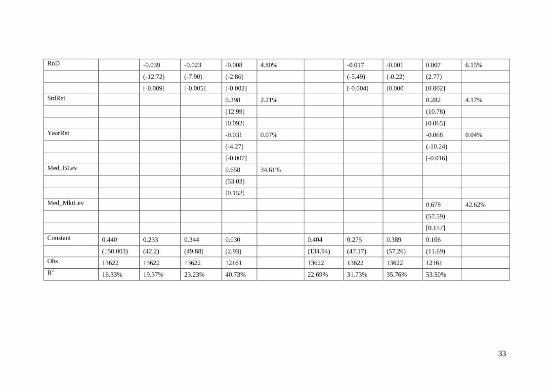
RnD -0.039 -0.023 -0.008 4.80% -0.017 -0.001 0.007 6.15%

(-12.72) (-7.90) (-2.86) (-5.49) (-0.22) (2.77)

[-0.009] [-0.005] [-0.002] [-0.004] [0.000] [0.002]

StdRet 0.398 2.21% 0.282 4.17%

(12.99) (10.78)

[0.092] [0.065]

YearRet -0.031 0.07% -0.068 0.04%

(-4.27) (-10.24)

[-0.007] [-0.016]

Med_BLev 0.658 34.61%

(53.03)

[0.152]

Med_MktLev 0.678 42.62%

(57.59)

[0.157]

Constant 0.440 0.233 0.344 0.030 0.404 0.275 0.389 0.106

(150.003) (42.2) (49.88) (2.93) (134.94) (47.17) (57.26) (11.69)

Obs 13622 13622 13622 12161 13622 13622 13622 12161

R2 16.33% 19.37% 23.23% 40.73% 22.69% 31.73% 35.76% 53.50%

34

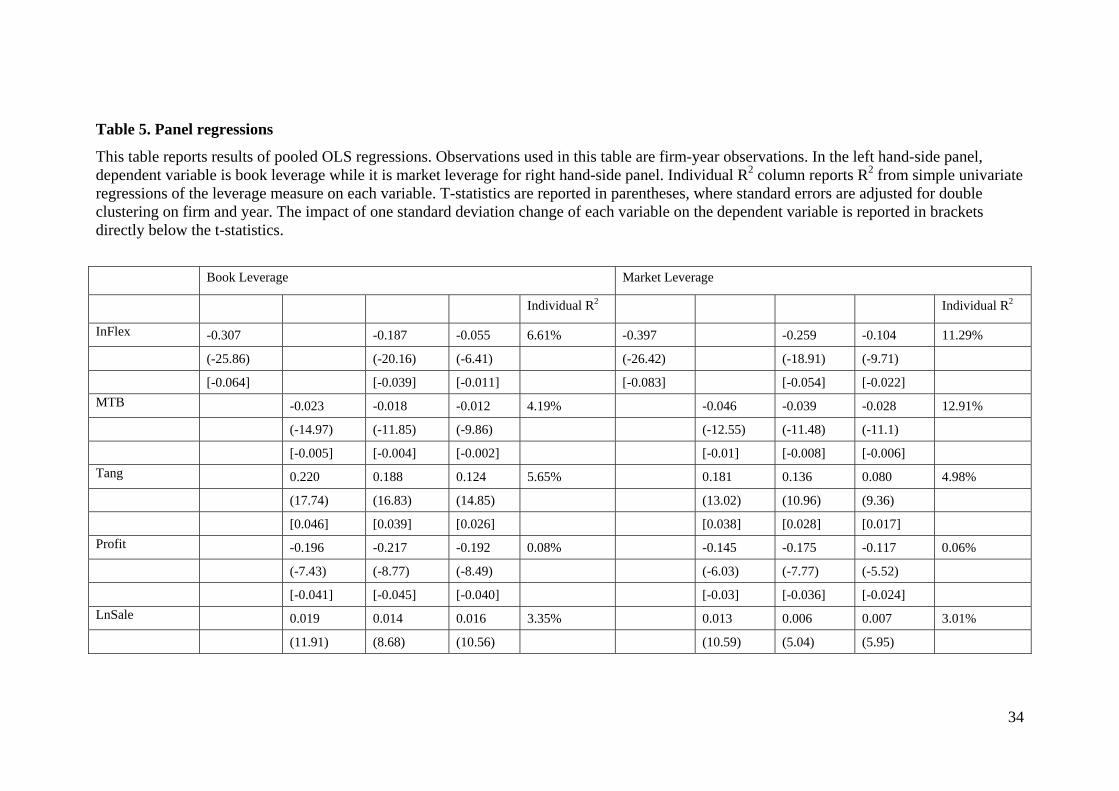
Table 5. Panel regressions

This table reports results of pooled OLS regressions. Observations used in this table are firm-year observations. In the left hand-side panel, dependent variable is book leverage while it is market leverage for right hand-side panel. Individual R2 column reports R2 from simple univariate regressions of the leverage measure on each variable. T-statistics are reported in parentheses, where standard errors are adjusted for double clustering on firm and year. The impact of one standard deviation change of each variable on the dependent variable is reported in brackets directly below the t-statistics.

Book Leverage Market Leverage

Individual R2 Individual R2

InFlex -0.307 -0.187 -0.055 6.61% -0.397 -0.259 -0.104 11.29%

(-25.86) (-20.16) (-6.41) (-26.42) (-18.91) (-9.71)

[-0.064] [-0.039] [-0.011] [-0.083] [-0.054] [-0.022]

MTB -0.023 -0.018 -0.012 4.19% -0.046 -0.039 -0.028 12.91%

(-14.97) (-11.85) (-9.86) (-12.55) (-11.48) (-11.1)

[-0.005] [-0.004] [-0.002] [-0.01] [-0.008] [-0.006]

Tang 0.220 0.188 0.124 5.65% 0.181 0.136 0.080 4.98%

(17.74) (16.83) (14.85) (13.02) (10.96) (9.36)

[0.046] [0.039] [0.026] [0.038] [0.028] [0.017]

Profit -0.196 -0.217 -0.192 0.08% -0.145 -0.175 -0.117 0.06%

(-7.43) (-8.77) (-8.49) (-6.03) (-7.77) (-5.52)

[-0.041] [-0.045] [-0.040] [-0.03] [-0.036] [-0.024]

LnSale 0.019 0.014 0.016 3.35% 0.013 0.006 0.007 3.01%

(11.91) (8.68) (10.56) (10.59) (5.04) (5.95)

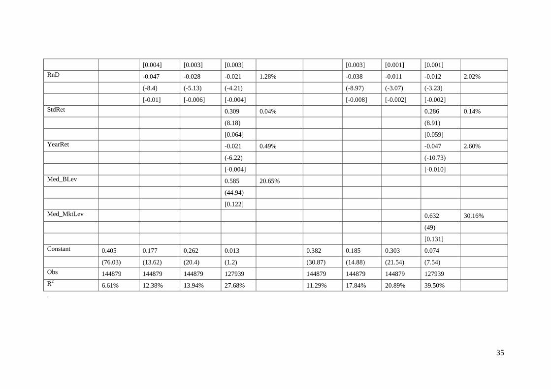
35

[0.004] [0.003] [0.003] [0.003] [0.001] [0.001]

RnD -0.047 -0.028 -0.021 1.28% -0.038 -0.011 -0.012 2.02%

(-8.4) (-5.13) (-4.21) (-8.97) (-3.07) (-3.23)

[-0.01] [-0.006] [-0.004] [-0.008] [-0.002] [-0.002]

StdRet 0.309 0.04% 0.286 0.14%

(8.18) (8.91)

[0.064] [0.059]

YearRet -0.021 0.49% -0.047 2.60%

(-6.22) (-10.73)

[-0.004] [-0.010]

Med_BLev 0.585 20.65%

(44.94)

[0.122]

Med_MktLev 0.632 30.16%

(49)

[0.131]

Constant 0.405 0.177 0.262 0.013 0.382 0.185 0.303 0.074

(76.03) (13.62) (20.4) (1.2) (30.87) (14.88) (21.54) (7.54)

Obs 144879 144879 144879 127939 144879 144879 144879 127939

R2 6.61% 12.38% 13.94% 27.68% 11.29% 17.84% 20.89% 39.50%

.

36

Table 6. Heterogeneous effects of InFlex

This table reports pooled OLS regressions results. Dependent variables are book leverage for the left hand-side panel and market leverage for the right hand-side panel. T-statistics are reported in parentheses, where standard errors are adjusted for double clustering on firm and year.

Book Leverage Market Leverage

InFlex -0.077 -0.021 -0.217 -0.184 -0.012 -0.205 -0.163 -0.342 -0.257 -0.213

(-4.51) (-0.88) (-16.86) (-17.75) (-0.45) (-10.98) (-6.53) (-24.85) (-18.82) (-8.33)

InFlex*NoDiv -0.162 -0.129 -0.084 -0.094

(-8.88) (-6.9) (-4.96) (-5.6)

NoDiv 0.119 0.102 0.091 0.092

(11.5) (10.29) (9.07) (9.32)

InFlex*NoRating -0.214 -0.173 -0.118 -0.097

(-9.06) (-6.96) (-4.66) (-3.81)

NoRating 0.100 0.102 -0.022 -0.023

(-10.09) (-9.52) (-1.31) (-1.38)

InFlex*MTB 0.037 0.055 0.104 0.120

(8.88) (14.66) (17.76) (17.01)

InFlex*Profit 0.367 0.287 0.300 0.354

(5.82) (5.81) (5.75) (7.22)

MTB -0.018 -0.019 -0.038 -0.016 -0.047 -0.039 -0.039 -0.095 -0.038 -0.102

(-11.46) (-12.68) (-16.18) (-12.1) (-19.86) (-11.41) (-11.66) (-18.23) (-11.61) (-17.9)

Tang 0.206 0.170 0.184 0.190 0.183 0.152 0.130 0.126 0.138 0.135

(19.76) (15.4) (17) (16.67) (17.58) (12.5) (10.89) (10.63) (10.95) (12.16)

37

Profit -0.206 -0.202 -0.200 -0.421 -0.326 -0.161 -0.171 -0.128 -0.341 -0.300

(-9.04) (-8.4) (-8.15) (-7.98) (-7.72) (-7.84) (-7.39) (-6.81) (-7.38) (-7.45)

LnSale 0.021 0.001 0.014 0.014 0.008 0.012 0.001 0.005 0.006 0.007

(13.94) (0.81) (8.46) (9.17) (4.14) (7.4) (0.77) (4.32) (5.3) (3.42)

RnD -0.016 -0.029 -0.038 -0.007 -0.018 -0.003 -0.011 -0.040 0.006 -0.015

(-3.65) (-5.85) (-7.34) (-1.73) (-4.83) (-0.84) (-3.21) (-8.29) (1.94) (-5.57)

Constant 0.154 0.417 0.276 0.261 0.344 0.216 0.347 0.343 0.302 0.305

(14.57) (33.25) (22.74) (20.15) (21.93) (14.3) (20.52) (25.75) (20.92) (19.86)

Obs 144879 144879 144879 144879 144879 144879 144879 144879 144879 144879

R2 16.00% 17.38% 14.37% 14.53% 20.08% 22.40% 21.36% 24.28% 21.30% 27.19%

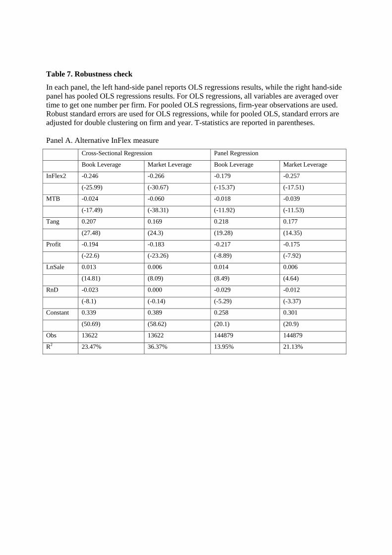
Table 7. Robustness check

In each panel, the left hand-side panel reports OLS regressions results, while the right hand-side panel has pooled OLS regressions results. For OLS regressions, all variables are averaged over time to get one number per firm. For pooled OLS regressions, firm-year observations are used. Robust standard errors are used for OLS regressions, while for pooled OLS, standard errors are adjusted for double clustering on firm and year. T-statistics are reported in parentheses. Panel A. Alternative InFlex measure

Cross-Sectional Regression Panel Regression

Book Leverage Market Leverage Book Leverage Market Leverage

InFlex2 -0.246 -0.266 -0.179 -0.257

(-25.99) (-30.67) (-15.37) (-17.51)

MTB -0.024 -0.060 -0.018 -0.039

(-17.49) (-38.31) (-11.92) (-11.53)

Tang 0.207 0.169 0.218 0.177

(27.48) (24.3) (19.28) (14.35)

Profit -0.194 -0.183 -0.217 -0.175

(-22.6) (-23.26) (-8.89) (-7.92)

LnSale 0.013 0.006 0.014 0.006

(14.81) (8.09) (8.49) (4.64)

RnD -0.023 0.000 -0.029 -0.012

(-8.1) (-0.14) (-5.29) (-3.37)

Constant 0.339 0.389 0.258 0.301

(50.69) (58.62) (20.1) (20.9)

Obs 13622 13622 144879 144879

R2 23.47% 36.37% 13.95% 21.13%

39

Panel B. Alternative leverage measure -- Debt to Total Assets

Cross-sectional regression Panel regression

D/A_Book D/A_Market D/A_Book D/A_Market

InFlex -0.171 -0.175 -0.129 -0.172

(-22.43) (-25.34) (-15.34) (-18.89)

MTB -0.020 -0.042 -0.014 -0.027

(-18.64) (-38.01) (-12.04) (-11.60)

Tang 0.169 0.132 0.181 0.140

(26.49) (22.40) (21.14) (15.23)

Profit -0.115 -0.118 -0.116 -0.106

(-18.20) (-20.37) (-7.06) (-6.88)

LnSale 0.006 0.003 0.005 0.002

(8.43) (4.82) (4.28) (2.01)

RnD -0.012 -0.001 -0.016 -0.009

(-5.42) (-0.39) (-4.28) (-3.28)

Constant 0.250 0.276 0.198 0.218

(47.36) (53.62) (20.10) (21.74)

Obs 13622 13622 144879 144879

R2 22.75% 33.16% 13.52% 19.58%

40

Panel C. Alternative leverage measure -- Net Leverage

Cross-sectional regression Panel regression

Net Book Leverage Net Market Leverage Net Book Leverage Net Market Leverage

InFlex -0.615 -0.451 -0.462 -0.355

(-31.14) (-30.21) (-16.11) (-17.51)

MTB -0.056 -0.017 -0.036 -0.018

(-16.91) (-8.32) (-11.98) (-5.77)

Tang 0.461 0.315 0.447 0.311

(37.09) (30.06) (21.37) (15.18)

Profit -0.150 -0.157 -0.166 -0.143

(-7.34) (-11.78) (-4.03) (-4.3)

LnSale 0.011 0.017 0.018 0.016

(7.54) (13.52) (7.73) (10.23)

RnD -0.112 -0.026 -0.092 -0.029

(-12.93) (-5.03) (-7.77) (-5.11)

Constant 0.213 0.127 0.067 0.084

(17.50) (11.58) (3.85) (5.1)

Obs 13622 13622 144874 144874

R2 42.99% 28.74% 25.44% 18.06%

41

Table 8. Comparison with other measures

Panel A and C present OLS regressions results while Panel B and D present pooled OLS regression results. Individual R2 column reports R2 from simple univariate regressions of the leverage measure on each variable. For OLS regressions, all variables are averaged over time to get one number per firm. For pooled OLS regressions, firm-year observations are used. Robust standard errors are used for OLS regressions, while for pooled OLS, standard errors are adjusted for double clustering on firm and year. T-statistics are reported in parentheses. In Panel A and B, the coefficients of SG&A/Sales are multiplied by 100. Panel A. Comparing to operating leverage -- Cross-sectional results

Book Leverage Market Leverage

Individual R2 Individual R2

InFlex -0.177 14.31% -0.206 21.28%

(-12.40) (-15.45)

MTB -0.034 -0.075

(-14.29) (-26.02)

Tang 0.204 0.147

(18.52) (14.30)

Profit -0.338 -0.320

(-18.91) (-18.74)

LnSale 0.013 0.006

(11.85) (6.19)

RnD -0.052 -0.017

(-7.17) (-2.33)

OPLev 0.147 0.068 0.194 0.072

(16.11) (7.43) (22.33) (8.83)

Constant 0.206 0.269 0.114 0.336

(28.71) (21.97) (17.3) (29.39)

Obs 7698 7698 7698 7698

R2 3.43% 25.07% 5.70% 38.21%

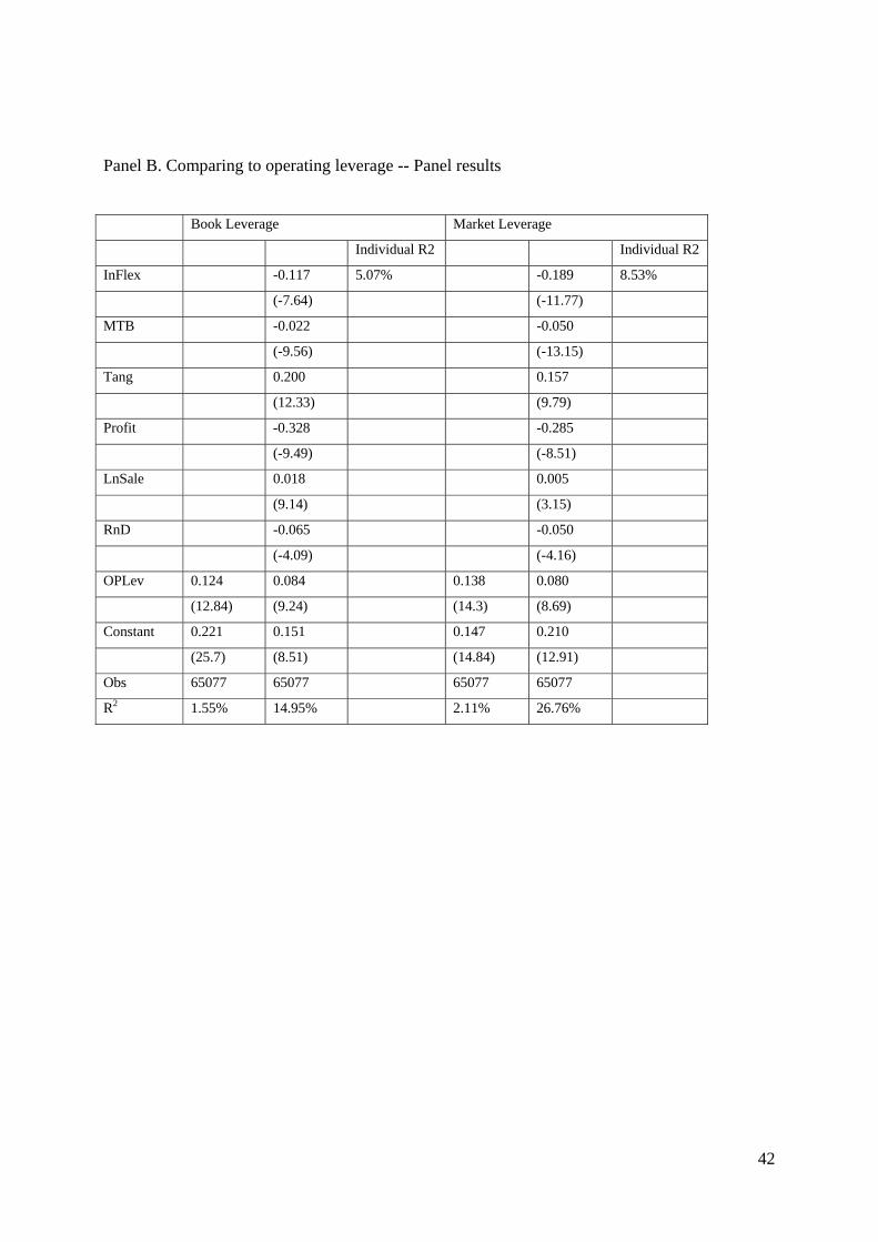
42

Panel B. Comparing to operating leverage -- Panel results

Book Leverage Market Leverage

Individual R2 Individual R2

InFlex -0.117 5.07% -0.189 8.53%

(-7.64) (-11.77)

MTB -0.022 -0.050

(-9.56) (-13.15)

Tang 0.200 0.157

(12.33) (9.79)

Profit -0.328 -0.285

(-9.49) (-8.51)

LnSale 0.018 0.005

(9.14) (3.15)

RnD -0.065 -0.050

(-4.09) (-4.16)

OPLev 0.124 0.084 0.138 0.080

(12.84) (9.24) (14.3) (8.69)

Constant 0.221 0.151 0.147 0.210

(25.7) (8.51) (14.84) (12.91)

Obs 65077 65077 65077 65077

R2 1.55% 14.95% 2.11% 26.76%

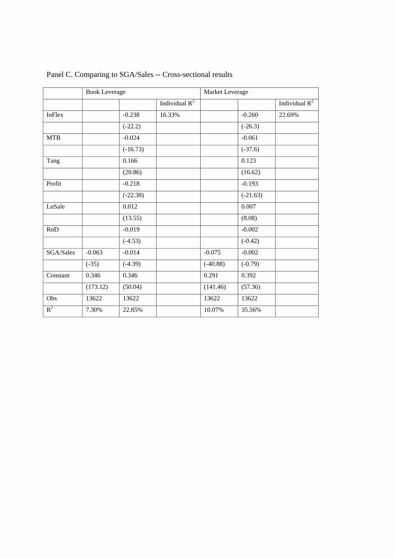
Panel C. Comparing to SGA/Sales -- Cross-sectional results Book Leverage Market Leverage

Individual R2 Individual R2

InFlex -0.238 16.33% -0.260 22.69%

(-22.2) (-26.3)

MTB -0.024 -0.061

(-16.73) (-37.6)

Tang 0.166 0.123

(20.86) (16.62)

Profit -0.218 -0.193

(-22.38) (-21.63)

LnSale 0.012 0.007

(13.55) (8.08)

RnD -0.019 -0.002

(-4.53) (-0.42)

SGA/Sales -0.063 -0.014 -0.075 -0.002

(-35) (-4.39) (-40.88) (-0.79)

Constant 0.346 0.346 0.291 0.392

(173.12) (50.04) (141.46) (57.36)

Obs 13622 13622 13622 13622

R2 7.30% 22.85% 10.07% 35.56%

44

Panel D. Comparing to SGA/Sales -- Panel results

Book Leverage Market Leverage

Individual R2 Individual R2

InFlex -0.187 6.61% -0.259 11.29%

(-16.64) (-18.94)

MTB -0.018 -0.039

(-11.89) (-11.5)

Tang 0.188 0.136

(16.83) (10.94)

Profit -0.217 -0.175

(-8.79) (-7.79)

LnSale 0.014 0.006

(8.66) (5.08)

RnD -5.370 -0.013

(-4.09) (-3.43)

SGA/Sales -0.025a 0.012 a -0.033 a 0.013 a

(-4.53) (3.27) (-4.38) (4.79)

Constant 0.311 0.261 0.260 0.302

(54.73) (20.33) (24.11) (21.52)

Obs 144879 144879 144879 144879

R2 0.04% 13.95% 0.06% 20.90%

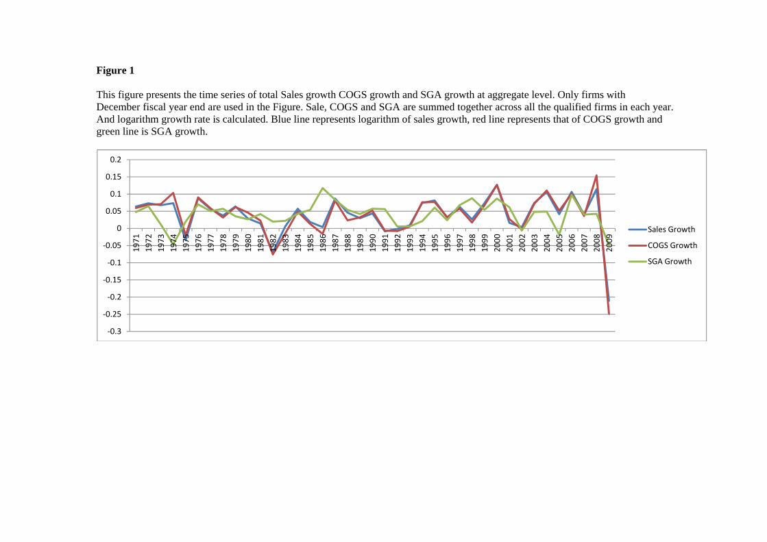
Figure 1 This figure presents the time series of total Sales growth COGS growth and SGA growth at aggregate level. Only firms with December fiscal year end are used in the Figure. Sale, COGS and SGA are summed together across all the qualified firms in each year. And logarithm growth rate is calculated. Blue line represents logarithm of sales growth, red line represents that of COGS growth and green line is SGA growth.

‐0.3

‐0.25

‐0.2

‐0.15

‐0.1

‐0.05

0

0.05

0.1

0.15

0.2

1971

1972

1973

1974

1975

1976

1977

1978

1979

1980

1981

1982

1983

1984

1985

1986

1987

1988

1989

1990

1991

1992

1993

1994

1995

1996

1997

1998

1999

2000

2001

2002

2003

2004

2005

2006

2007

2008

2009

Sales Growth

COGS Growth

SGA Growth