CorridorDesigner ArcGIS Toolbox Tutorial

corridordesign.org

Dan Majka

Paul Beier

Jeff Jenness

The CorridorDesigner project is funded by a generous grant from the Environmental Research, Development and Education for the New Economy (ERDENE) initiative from Northern Arizona University.

Our approach was initially developed during 2001-2006 for South Coast

Missing Linkages, a set of 16 linkage designs in southern California (draft &

final designs at scwildlands.org). Kristeen Penrod, Clint Cabañero, Wayne

Spencer, and Claudia Luke made enormous contributions to SCML and the

procedures in CorridorDesigner.

Our approach was modified for the Arizona Missing Linkages Project,

supported by Arizona Game and Fish Department, Arizona Department of

Transportation, U.S. Fish and Wildlife Service, U.S. Forest Service, Federal

Highway Administration, Bureau of Land Management, Sky Island Alliance,

Wildlands Project, and Northern Arizona University.

Over the past 5 years, we discussed these ideas with Andrea Atkinson, Todd

Bayless, Clint Cabañero, Liz Chattin, Matt Clark, Kevin Crooks, Kathy Daly,

Brett Dickson, Robert Fisher, Emily Garding, Madelyn Glickfeld, Nick Haddad,

Steve Loe, Travis Longcore, Claudia Luke, Lisa Lyren, Brad McRae, Scott

Morrison, Shawn Newell, Reed Noss, Kristeen Penrod, E.J. Remson, Seth

Riley, Esther Rubin, Ray Sauvajot, Dan Silver, Jerre Stallcup, and Mike White.

We especially thank the many government agents, conservationists, and

funders who conserve linkages and deserve the best possible science.

3

TERMS & CONDITIONS By downloading or using any of the CorridorDesigner GIS tools, you agree to the following terms and

conditions:

These tools are available to assist in identifying general areas of concern only. Results obtained by the tools

provided should only be relied upon with corroboration of the methods, assumptions, and results by a qualified

independent source.

The user assumes full responsibility for the misinterpretation or manipulation of the data. The user of this

information shall indemnify and hold free the Northern Arizona University, the State of Arizona, and the

creators of the CorridorDesigner GIS tools from any and all liabilities, damages, lawsuits, and causes of action

that result as a consequence of his/her reliance on information provided herein or from any misinterpretation or

manipulation of the data.

LICENSE These tools are distributed under a Creative Commons Attribution-ShareAlike 3.0

Unported license. According to the terms of this license, you are free to copy, change and

redistribute the tools. If you alter, transform, or build upon this work, you may distribute the resulting work

only under the same, similar or a compatible license. More information about this license can be found at

http://creativecommons.org/licenses/by-sa/3.0/

CREDITS The CorridorDesigner project is funded by a generous grant from the Environmental Research, Development

and Education for the New Economy (ERDENE) initiative from Northern Arizona University.

Our approach was initially developed during 2001-2006 for South Coast Missing Linkages, a set of 16 linkage

designs in southern California (draft & final designs at scwildlands.org). Kristeen Penrod, Clint Cabañero,

Wayne Spencer, and Claudia Luke made enormous contributions to SCML and the procedures in

CorridorDesigner.

Our approach was modified for the Arizona Missing Linkages Project, supported by Arizona Game and Fish

Department, Arizona Department of Transportation, U.S. Fish and Wildlife Service, U.S. Forest Service,

Federal Highway Administration, Bureau of Land Management, Sky Island Alliance, Wildlands Project, and

Northern Arizona University.

4

Over the past 5 years, we discussed these ideas with Andrea Atkinson, Todd Bayless, Clint Cabañero, Liz

Chattin, Matt Clark, Kevin Crooks, Kathy Daly, Brett Dickson, Robert Fisher, Emily Garding, Madelyn

Glickfeld, Nick Haddad, Steve Loe, Travis Longcore, Claudia Luke, Lisa Lyren, Brad McRae, Scott Morrison,

Shawn Newell, Reed Noss, Kristeen Penrod, E.J. Remson, Seth Riley, Esther Rubin, Ray Sauvajot, Dan Silver,

Jerre Stallcup, and Mike White. We especially thank the many government agents, conservationists, and

funders who conserve linkages and deserve the best possible science.

5

TABLE OF CONTENTS TE R M S & CO N D I TI O N S . . . . . . . . . . . . . . . . . . . . . . . . . . . . . . . . . . . . . . . . . . . . . . . . . . . . . . . . . . . . . . . . . . . . . . . . . . . . . . . . . . . . . . . . . . 3

LI C E NS E . . . . . . . . . . . . . . . . . . . . . . . . . . . . . . . . . . . . . . . . . . . . . . . . . . . . . . . . . . . . . . . . . . . . . . . . . . . . . . . . . . . . . . . . . . . . . . . . . . . . . . . . . . . . . . 3

CR E DI T S . . . . . . . . . . . . . . . . . . . . . . . . . . . . . . . . . . . . . . . . . . . . . . . . . . . . . . . . . . . . . . . . . . . . . . . . . . . . . . . . . . . . . . . . . . . . . . . . . . . . . . . . . . . . . 3

TA B L E O F CO N T E N TS . . . . . . . . . . . . . . . . . . . . . . . . . . . . . . . . . . . . . . . . . . . . . . . . . . . . . . . . . . . . . . . . . . . . . . . . . . . . . . . . . . . . . . . . . . . . 5

PRE P A RI NG F O R A N A L YSIS . . . . . . . . . . . . . . . . . . . . . . . . . . . . . . . . . . . . . . . . . . . . . . . . . . . . . . . . . . . . . . . . . . . . . . . . . . . . . . . . . . . . . . 8 Introduction to the tutorial dataset ................................................................................................................8 Setting up a project directory and naming conventions ..................................................................................8

Copying the tutorial data .....................................................................................................................8 Creating an analysis directory structure ................................................................................................8 Naming conventions ............................................................................................................................9 Log files ...............................................................................................................................................9

Defining the analysis area and wildland blocks...............................................................................................9 Adding the CorridorDesigner toolbox............................................................................................................11 Clipping analysis layers ..................................................................................................................................12 Creating a topographic position raster............................................................................................................13 Creating a distance-from-roads raster .............................................................................................................14

MO D EL I N G H A BI T A T . . . . . . . . . . . . . . . . . . . . . . . . . . . . . . . . . . . . . . . . . . . . . . . . . . . . . . . . . . . . . . . . . . . . . . . . . . . . . . . . . . . . . . . . . . . . . 15 Creating species factor reclassification files .....................................................................................................15 Creating a habitat suitability model ...............................................................................................................17 Creating a habitat patch map .........................................................................................................................19

MO D EL I N G C O RR I DO R S . . . . . . . . . . . . . . . . . . . . . . . . . . . . . . . . . . . . . . . . . . . . . . . . . . . . . . . . . . . . . . . . . . . . . . . . . . . . . . . . . . . . . . . . . 21 Creating a corridor model..............................................................................................................................21 Creating corridor slices ..................................................................................................................................23

GU I D E T O CO R R ID O RDE S I G N E R O U T P U T . . . . . . . . . . . . . . . . . . . . . . . . . . . . . . . . . . . . . . . . . . . . . . . . . . . . . . . . . . . . . . . . . . 24

6

CorridorDesigner requires ArcGIS 9.1 or 9.2 with the

Spatial Analyst extension activated. The current release

of the CorridorDesigner toolbox must be used in

ArcCatalog. We are working on a version that runs

correctly in ArcMap.

This short tutorial documents CorridorDesigner’s main

tools; for additional documentation, please see the in-

tool help, available by clicking the help button within

each tool.

7

8

PREPARING FOR ANALYSIS Introduction to the tutorial dataset

This tutorial uses data from one linkage design

created for Arizona Missing Linkages, a two-year

project funded by the Arizona Game and Fish

Department which produced 16 linkage designs

throughout Arizona. The linkage aimed to connect

two large wildland blocks managed by the U.S.

Forest Service. The southwestern wildland block

(hereafter: Tumacacori wildland block) includes

over 200,000 acres within the Coronado National

Forest, plus the adjoining 118,000 acre Buenos

Aires National Wildlife Refuge. The northeastern

wildland block (hereafter: Santa Rita wildland

block) consists of 173,000 acres of Coronado

National Forest, the 53,000-acre Santa Rita

Experimental Range and Wildlife Refuge, the

BLM-administered 45,000-acre Las Cienegas

Natural Conservation Area, the 5,000 acre

Patagonia Lake State Park, and the Nature

Conservancy’s 1,350-acre Patagonia-Sonoita Creek

Preserve.

While the Arizona Missing Linkages project

modeled 19 species for this linkage design, we will

be focusing on just one–black bear.

All data required for the tutorial are found in the

accompanying zip file available on

http://corridordesign.org/downloads.

Within the zip file are three folders:

basemap includes all GIS data, in NAD UTM

83 z12 projection. Land cover was derived

from the Southwest ReGAP land cover data

set, elevation was derived from the NED

DEM, and most vector layers came from

Arizona Land Resource Information System

(ALRIS).

output is an empty directory to use for storing

model outputs

speciesData: includes parameterizations for five

species

layerFiles: includes ArcGIS .lyr files for

symbolizing habitat suitability, patch maps,

and topographic position

Setting up a project directory and naming conventions

While everyone manages GIS projects differently,

we suggest creating a uniform directory structure

and naming conventions for managing analysis

layers. It is not uncommon to create 20-30 data

layers for each species modeled in an analysis–if

modeling more than a species or two, data

management gets messy quickly.

CO P Y I N G T HE T U T OR I AL D A T A

1. To work through the tutorial, download and

extract the CD_toolbox_tutorial_data.zip file to

your local hard drive.

CR E A T I N G A N A N A L Y S I S D I R E C TO R Y

S T R U C T U R E

1. Within the tutorial directory, you will find a folder

named basemap and a folder named output. All

input GIS layers–such as land cover, elevation,

9

roads, and wildland blocks–are saved in the

basemap folder. All modeling output–such as

habitat suitability models, habitat patch maps, and

corridor models–will be saved in the output folder.

NA M I N G CON V E N T IO N S

All CorridorDesigner output is in the form of

shapefiles and ESRI rasters. While shapefiles

support long file names, rasters are limited to 13

characters. We recommend the following naming

conventions:

Do not use spaces in the output directory path

or filenames

For tools requiring species name as a

parameter, limit the name to 9 characters with

no spaces.

LO G F IL E S

One of the great additions to geoprocessing in

ArcGIS 9.x is the ability to use the command line

to run tools in ArcToolbox. While all examples in

this tutorial show the CorridorDesigner dialog

boxes, CorridorDesigner also creates a text log file

every time a tool is run which saves the command

line syntax for the tool. This makes the tool easy to

re-run, and is useful for reviewing what parameters

were used in any given analysis.

Defining the analysis area and wildland blocks

NOTE: The analysis area and wildland blocks have

already been created and saved to the basemap folder

for this tutorial. You will need to repeat these steps

when using CorridorDesigner with your own data set.

1. Navigate to the folder where you copied the

tutorial data, and under the path \tutorial\, open

CorridorDesigner_tutorial.mxd.

2. In ArcCatalog, create a new empty polygon

shapefile named “analysis_area.shp,” and save it in

the \tutorial \basemap folder. Set the projection to

NAD_1983_UTM_Zone_12N. If you do not

know how to create a new shapefile in ArcCatalog,

open the ArcGIS help by selecting “ArcGIS

Desktop Help” under the Help menu, and search

for creating new shapefiles.

3. Add analysis_area.shp to ArcMap by clicking the

Add Data button on the Standard toolbar.

4. Define the analysis area. In ArcMap, make sure the

editing toolbar is turned on (View > Toolbars >

Editor). Start an editing session on

analysis_area.shp, select the Sketch Tool on the

Editor toolbar, and draw a rectangle around the

Santa Rita Mtns USFS block, the Tumacacori-

Atascosa Mtns USFS block, and the Buenos Aires

NWR block. Stop the editing session and save

your changes: the rectangle you just saved will be

your analysis area.

5. Creating wildland block 1. Set the ownership layer

as the only selectable layer (Selection > Set

Selectable Layers > Click ownership on). From the

ownership file select the Santa Rita Mtns USFS

block. Right-click the ownership layer in the Table

of Contents, and select Data > Export Data.

Export the selection to a new shapefile named

SantaRita_WildlandBlock.shp, saving it in the

\tutorial \basemap folder. This will be the Santa

Rita Wildland Block.

10

6. Creating wildland block 2. Repeat the procedures

from step 5 to create wildland block 2. From the

ownership file select the Tumacacori-Atascosta

Mtns USFS block and the Buenos Aires NWR

blocks. Export the selections to a new shapefile

named Tumacacori_WildlandBlock.shp, saving it

in the \tutorial \basemap folder. This will be the

Tumacacori Wildland Block.

11

Adding the CorridorDesigner toolbox

Now that we have defined the analysis area and

wildland blocks, we will use CorridorDesigner to

prepare data layers for analysis. First, we need to

add the CorridorDesigner toolbox to ArcToolbox.

ArcToolbox can be used

in both ArcMap and

ArcCatalog. Adding the

CorridorDesigner

toolbox to ArcToolbox

follows the same

procedure in both

programs. Throughout

this tutorial, we will

conduct modeling in

ArcCatalog, and view the

results in ArcMap.

1. Show the ArcToolbox

window by clicking the

ArcToolbox button.

2. Right-click the

ArcToolbox folder inside

the ArcToolbox window

and click Add Toolbox.

3. Click the Look in dropdown arrow and navigate to

the location of the CorridorDesigner toolbox. By

default, this is found under

CorridorDesigner\tools.

4. Click the toolbox.

5. Click open. The CorridorDesigner toolbox is

added to the ArcToolbox window.

6. Make sure the Spatial Analyst extension is

activated: Go to Tools > Extensions, and ensure

Spatial Analyst is checked on.

12

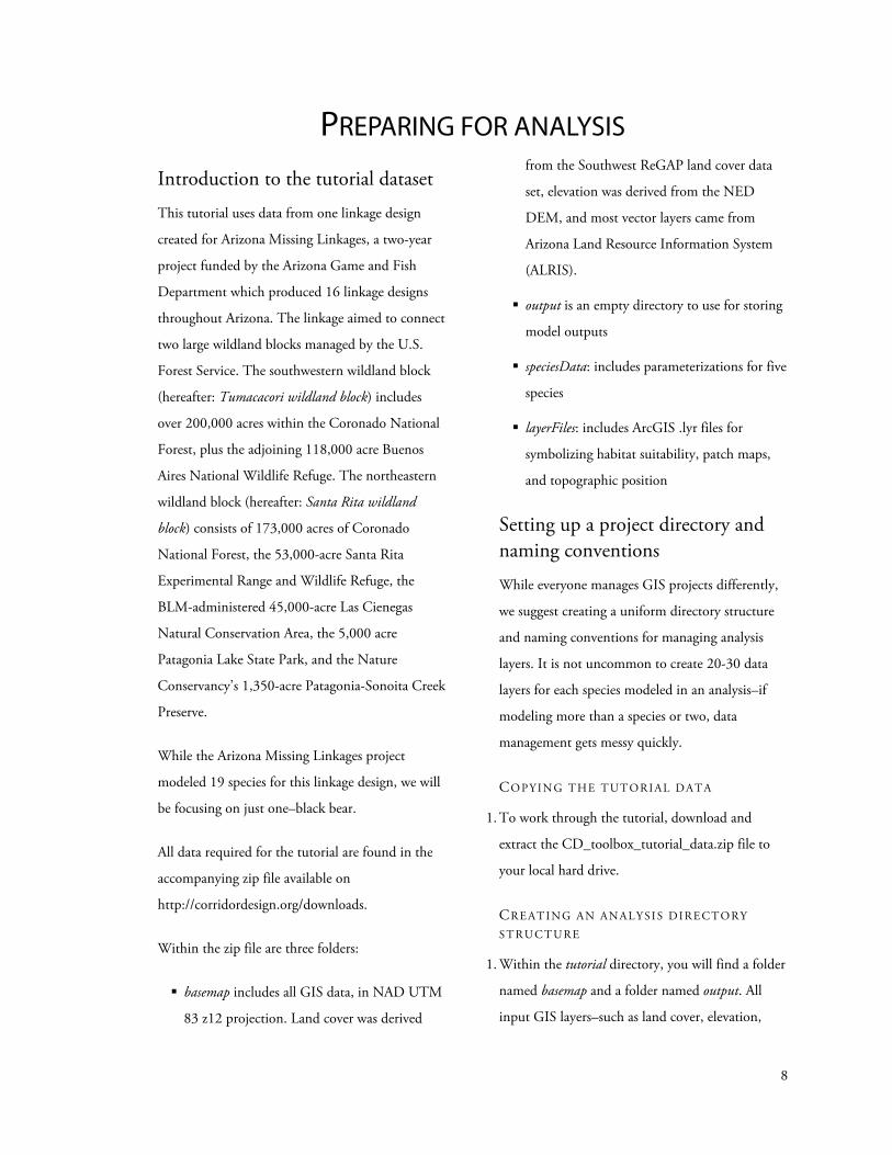
Clipping analysis layers

NOTE: Analysis layers have already been clipped and

saved to the basemap folder for this tutorial. You will

need to repeat these steps when using

CorridorDesigner with your own data set. For now,

you can skip to the next step, Creating a topographic

position raster.

Once the analysis area and wildland blocks have

been defined, we need to gather all relevant GIS

layers that will be used in the analysis, and clip

these layers to the analysis area. While statewide or

large regional datasets can be used without clipping

them to the analysis area, clipping all data to the

analysis area improves processing time, reduces the

size of layers created during the modeling process,

and creates a convenient stand-alone project which

can be shared with partners.

1. Within CorridorDesigner, expand the I. Layer

Preparation toolbox, and double-click the first

tool, 1) Clip layers to analysis area

2. Add the analysis area shapefile into the first

parameter box.

3. We want to save all of the clipped layers into the

\projects \basemap folder. Add this folder to the

second parameter box.

4. The clip layers tool accepts two types of inputs:

vector data, such as shapefiles and feature classes,

and raster data, such as the elevation and land

cover grids. In the third parameter box, add all of

the supplied vector data, found in:

\CorridorDesigner\statewide\basemap

5. To clip the two statewide raster layers to the

analysis area, add aml_landcover and dem_m to

the fourth parameter box. These are found in

\CorridorDesigner\tutorial\data\statewide\raster.

6. Click OK.

7. When the tool has finished, browse to the

\tutorial\basemap folder. Right-click on the folder,

and click Refresh. If you preview these layers, you

will see that they have been clipped to the analysis

area.

8. At this point, we will no longer work with any of

the statewide data. Make sure that for any further

analyses in the tutorial, you use the clipped layers,

found in the \tutorial\basemap folder. Failure to

do so may result in long processing times and a

cranky computer!

13

Creating a topographic position raster

1. Double-click the 2) Create topographic position

raster tool to open it.

2. Add the clipped elevation raster, found in \tutorial

\basemap\dem_m

3. Name the output raster topo, and save it in the

tutorial\basemap folder.

4. The default parameters in this tool were used for

the Arizona Missing Linkages project. In a

nutshell, the parameters say: “Compared to all of

the pixels found in a 200m radius surrounding a

given pixel:

the pixel will be classified as a canyon bottom if

the pixel has an elevation at least 12m less

than the average of the neighborhood pixels

the pixel will be classified as a ridgetop if the

pixel has an elevation at least 12m greater than

the average of the neighborhood pixels

the pixel will be classified as a flat-gentle slope

if the pixel is not classified as a canyon bottom

or ridgetop, and has a slope less than 6 degrees

the pixel will be classified as a steep slope if the

pixel is not classified as a canyon bottom or

ridgetop, and has a slope more than 6 degrees

5. We will accept these default parameters. Press OK

to run the tool.

6. In the output topographic position raster,

topographic positions are given numeric codes

using the VALUE attribute:

1 is a canyon bottom

2 is a flat-gentle slope

3 is a steep slope

4 is a ridgetop

7. We have included a layer file, located in \tutorial

\layerFiles\TopographicPosition.lyr to symbolize

this.

8. To review how well the topographic position raster

characterized the landscape, it is useful to view it in

conjunction with a hillshade. Create a hillshade

using the hillshade tool found in the Spatial

Analyst > Surface toolbox. Add the hillshade to

14

ArcMap on top of the topographic position raster,

and set its transparency to 60%. How does the

topographic position raster look?

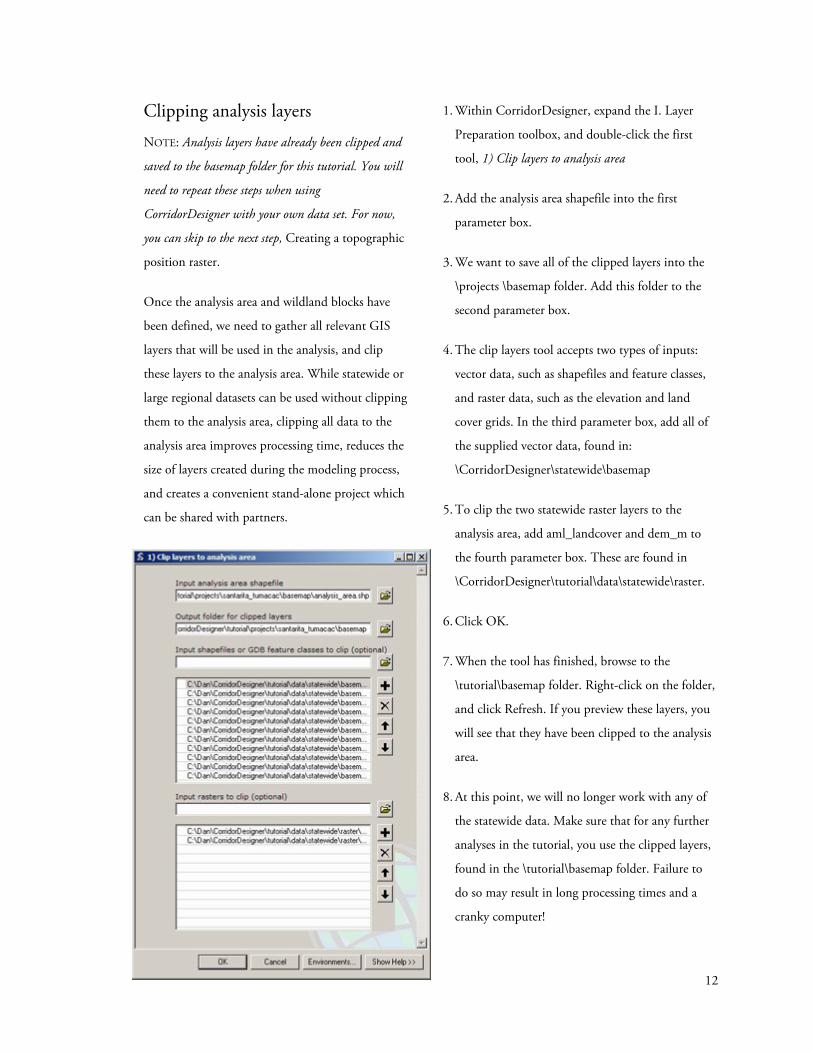
Creating a distance-from-roads raster

In order to create habitat models, we have one

more raster to create–a distance from roads layer.

To do this we will use a standard tool found in the

Spatial Analyst toolbox.

1. Open the Euclidean Distance tool, found in the

Distance toolset of the Spatial Analyst Tools

toolbox.

2. Select the clipped roads shapefile, found in

\tutorial\basemap for the first parameter, Input

raster or feature source data,

3. Name the output distance raster dstroad, and

save it in the \tutorial\basemap folder.

4. We want the output distance from roads raster

to have the same cell size (30m) as the elevation

model. Select the clipped elevation model,

dem_m, found in the \tutorial\basemap folder,

for the fourth parameter, Output cell size.

5. Click OK.

15

MODELING HABITAT With the analysis area and wildland blocks

defined, and the necessary GIS layers clipped and

created, we are now ready to create habitat

suitability models.

CorridorDesigner provides three tools for creating

habitat suitability models. For this tutorial, we will

concentrate on the primary tool. Details on how to

use the other two tools, which a) combine

previously reclassified habitat factors into a

suitability model, and b) normalize an existing

suitability model into a 0-100 framework, can be

found within the in-tool help for each.

Creating species factor reclassification files

CorridorDesigner uses reclassification text files to

build habitat suitability models. While developing

these text files may initially seem cumbersome,

once created, they can be reused for many habitat

or corridor analyses. For this tutorial, we have

provided data for 12 species. To understand the

format of these text files, we’ll work with data for

the black bear.

1. Browse to \tutorial\ speciesData\blackbear

2. In this folder you will find 6 text files and 1

Microsoft Excel spreadsheet. The Excel spreadsheet

is the original habitat model filled out by a species

expert. We will not be using it in this tutorial, but

you may find it useful to look at. The 6 text files

are:

blackbear_dstroad.txt: distance-from-roads reclass file

blackbear_elev_m.txt: elevation (in meters) reclass file

blackbear_lndcvr.txt: land cover reclass file

blackbear_topo.txt: topographic position reclass file

blackbear_weights.txt: weights assigned to each of 4 habitat factors

blackbear_patches.txt: patch size information

3. Open the distance-from-roads reclass file. This file

shows the required format for reclassifying

continuous variables such as distance-from-roads

and elevation. This file is simply a tab-delineated

text file, with the continuous variable range on the

left, a colon, and the suitability score on the right.

The file can be read as, “From 0 to 100 meters

away from a road, the suitability score for black

bear is 11. Between 100 and 500 meters away from

a road, the suitability score is 67. Farther than 500

meters away from a road, the suitability score is

100.

4. Open _elev_m.txt. You will see that this file looks

very similar to the roads reclass file, only the

numbers on the left correspond to elevation in

meters. The reclassification ranges in the elevation

16

text file have odd intervals because they were

originally provided by the species expert as

elevation in feet, which we converted to meters.

Note: When constructing distance-from-road or

elevation reclass text files, make sure the reclass

range encompasses all the possible values in your

analysis area. For example, if there are 3,000 m

mountains in your analysis area, provide a score up

to 3000m (e.g. 2000 3000 : 75). If there are

pixels in your study area that are 30,000m from a

road, make sure your reclass range goes up to

30,000m.

5. Open blackbear_lndcvr.txt. This file shows the

required format for reclassifying categorical

variables. The values on the left correspond to the

VALUE attribute of the supplied land cover raster,

while the values on the right correspond to the

suitability score assigned to each land cover value.

Again, this file is constructed by creating a simple

tab-delineated text file.

Because these values are a bit mysterious without

their corresponding land cover name (and ArcGIS

drops all attributes except for VALUE when a

raster is clipped), we have supplied a table which

can be joined to the land cover grid to display

names. This table is found here:

\tutorial\statewide\aml_landcover.dbf.

6. Open blackbear_topo.txt. You will see that this file

looks similar to the land cover reclass file, only

there are just 4 values which correspond to the

topographic position categories discussed above.

Note: When constructing reclassification text files,

all values must go in ascending numerical order

(e.g. 1,2,3,4,5, NOT 1,3,2,5,4). The tool will fail

if all values are not in ascending numerical order.

17

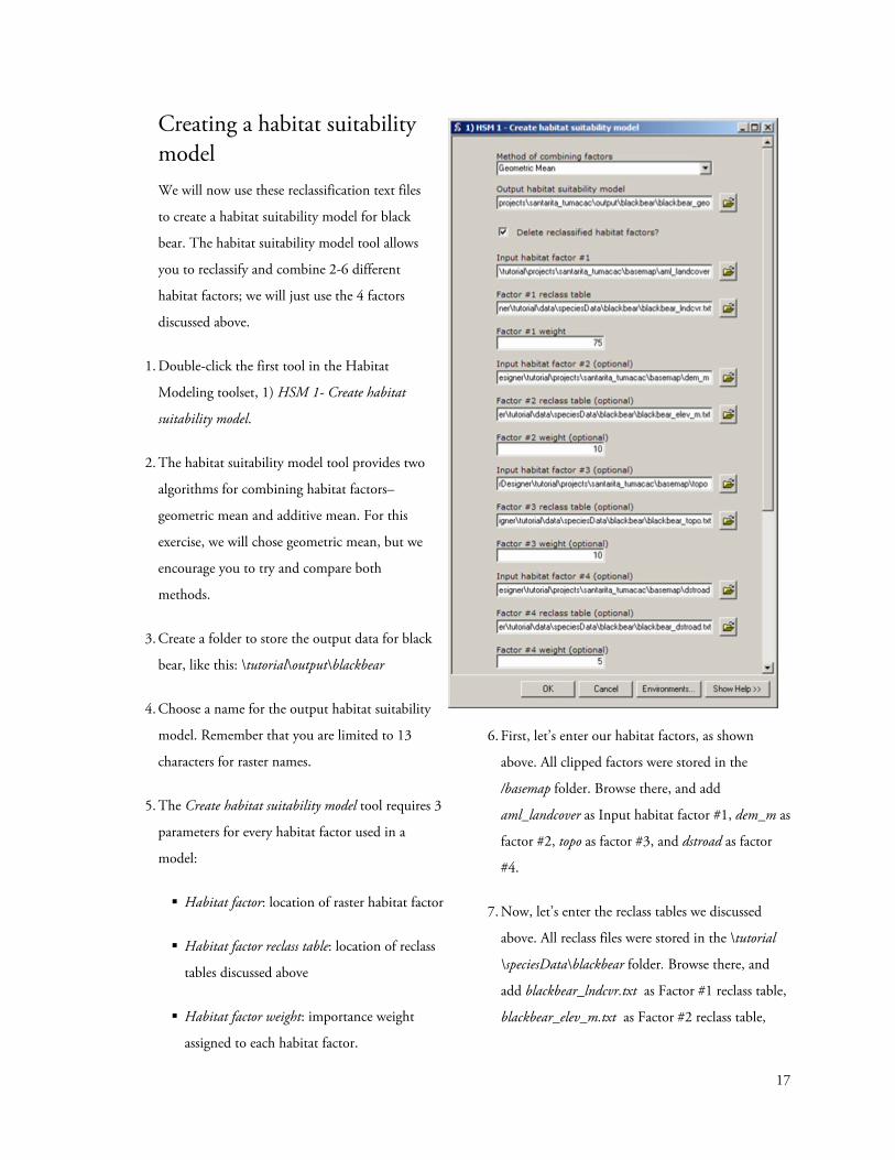
Creating a habitat suitability model We will now use these reclassification text files

to create a habitat suitability model for black

bear. The habitat suitability model tool allows

you to reclassify and combine 2-6 different

habitat factors; we will just use the 4 factors

discussed above.

1. Double-click the first tool in the Habitat

Modeling toolset, 1) HSM 1- Create habitat

suitability model.

2. The habitat suitability model tool provides two

algorithms for combining habitat factors–

geometric mean and additive mean. For this

exercise, we will chose geometric mean, but we

encourage you to try and compare both

methods.

3. Create a folder to store the output data for black

bear, like this: \tutorial\output\blackbear

4. Choose a name for the output habitat suitability

model. Remember that you are limited to 13

characters for raster names.

5. The Create habitat suitability model tool requires 3

parameters for every habitat factor used in a

model:

Habitat factor: location of raster habitat factor

Habitat factor reclass table: location of reclass

tables discussed above

Habitat factor weight: importance weight

assigned to each habitat factor.

6. First, let’s enter our habitat factors, as shown

above. All clipped factors were stored in the

/basemap folder. Browse there, and add

aml_landcover as Input habitat factor #1, dem_m as

factor #2, topo as factor #3, and dstroad as factor

#4.

7. Now, let’s enter the reclass tables we discussed

above. All reclass files were stored in the \tutorial

\speciesData\blackbear folder. Browse there, and

add blackbear_lndcvr.txt as Factor #1 reclass table,

blackbear_elev_m.txt as Factor #2 reclass table,

18

blackbear_topo.txt as Factor #3 reclass table, and

blackbear_dstroad.txt as Factor #1 reclass table.

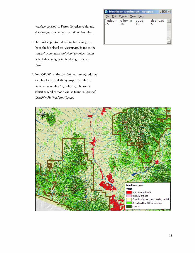
8. Our final step is to add habitat factor weights.

Open the file blackbear_weights.txt, found in the

\tutorial\data\speciesData\blackbear folder. Enter

each of these weights in the dialog, as shown

above.

9. Press OK. When the tool finishes running, add the

resulting habitat suitability map to ArcMap to

examine the results. A lyr file to symbolize the

habitat suitability model can be found in \tutorial

\layerFiles\HabitatSuitability.lyr.

19

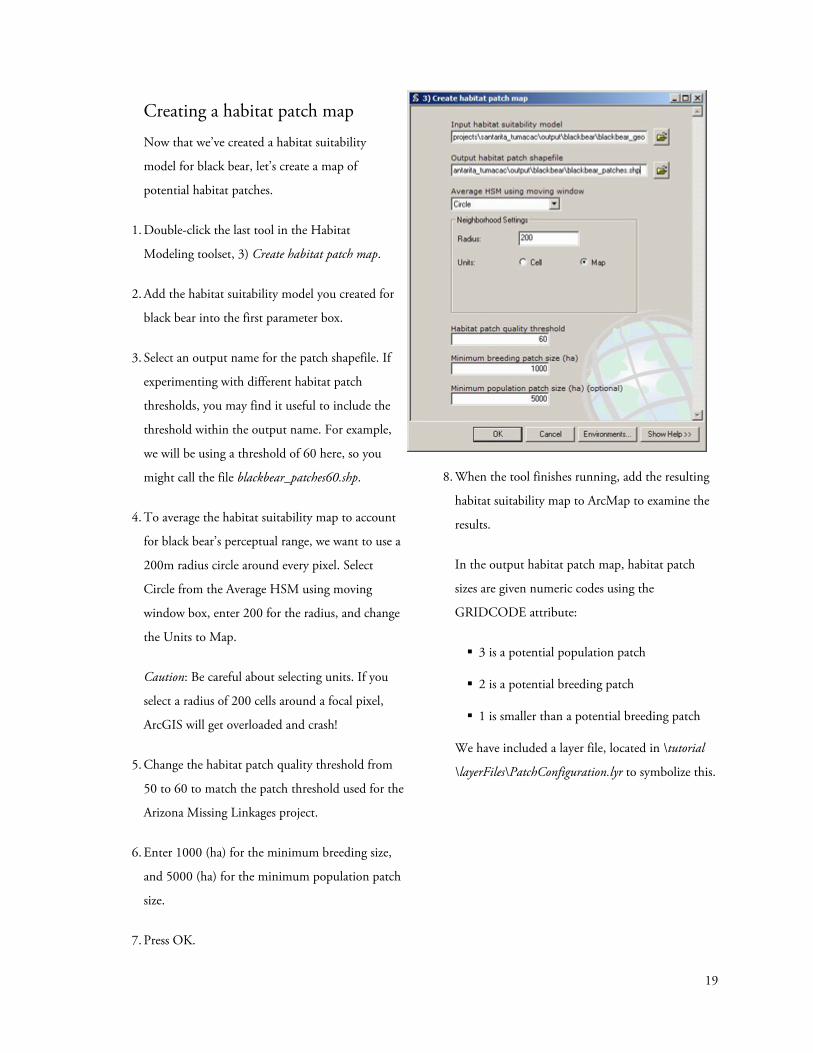
Creating a habitat patch map

Now that we’ve created a habitat suitability

model for black bear, let’s create a map of

potential habitat patches.

1. Double-click the last tool in the Habitat

Modeling toolset, 3) Create habitat patch map.

2. Add the habitat suitability model you created for

black bear into the first parameter box.

3. Select an output name for the patch shapefile. If

experimenting with different habitat patch

thresholds, you may find it useful to include the

threshold within the output name. For example,

we will be using a threshold of 60 here, so you

might call the file blackbear_patches60.shp.

4. To average the habitat suitability map to account

for black bear’s perceptual range, we want to use a

200m radius circle around every pixel. Select

Circle from the Average HSM using moving

window box, enter 200 for the radius, and change

the Units to Map.

Caution: Be careful about selecting units. If you

select a radius of 200 cells around a focal pixel,

ArcGIS will get overloaded and crash!

5. Change the habitat patch quality threshold from

50 to 60 to match the patch threshold used for the

Arizona Missing Linkages project.

6. Enter 1000 (ha) for the minimum breeding size,

and 5000 (ha) for the minimum population patch

size.

7. Press OK.

8. When the tool finishes running, add the resulting

habitat suitability map to ArcMap to examine the

results.

In the output habitat patch map, habitat patch

sizes are given numeric codes using the

GRIDCODE attribute:

3 is a potential population patch

2 is a potential breeding patch

1 is smaller than a potential breeding patch

We have included a layer file, located in \tutorial

\layerFiles\PatchConfiguration.lyr to symbolize this.

20

21

MODELING CORRIDORS Creating a corridor model

You will notice that the Create corridor model tool

requires many of the same parameters as the Create

habitat patch map tool. This is because

CorridorDesigner recalculates a patch map within

each of the wildland blocks. CorridorDesigner uses

the patch map within each wildland block to

determine starting and ending points for the

corridor. It first attempts to use all population

patches within a wildland block as starting points;

if there are no population patches, it selects any

breeding patches to use as starting points. If there

are no breeding patches, CorridorDesigner will

select any available habitat patches; however, you

may want to reconsider if a corridor model is

appropriate if there are not at least potential

breeding patches within both wildland blocks.

1. Double-click the first tool in the Corridor

Modeling toolset, 1) Create corridor model.

2. Add the habitat suitability model you created for

black bear into the first parameter box.

3. Select the Tumacacori and Santa Rita wildland

blocks you previously created, and add them to the

second and third parameter boxes. Note: The input

order of these protected blocks will not affect the

analysis. Either the Tumacacori or the Santa Rita

wildland block can be wildland block #1–just

make sure you do not input the same wildland

block for both wildland blocks #1 and #2!

4. Because the Create corridor model tool creates many

output layers, you must select a folder in which to

save the output layers, and a base species name to

append to all output files. For Output workspace,

select the output folder for black bear: \tutorial

\output\blackbear. For species name, input blackbear,

making sure there are no spaces between words.

5. Enter the habitat patch information for black bear

you used in the previous exercise, Creating a habitat

patch map.

6. Press OK.

22

7. When the tool finishes running, browse to the black

bear output folder using ArcCatalog to examine the

output.

The Create corridor model tool creates several

output layers:

corridor slices: denoted by the species name,

and _x_x_percent_corridor.shp. The numbers

x_x refer to the percent of the landscape

contained within the corridor slice. For

example, the 0_1_percent_corridor is the

most permeable 0.1% of the landscape

connecting the wildland blocks.

3_0_percent_corridor is the most permeable

3.0% of the landscape. By default, the Create

corridor model tool creates slices ranging from

0.1-10.0% of the landscape. To create

additional corridor slices, use the tool Create

corridor slices.

Cumulative cost grid: denoted by the species

name and _cst. This grid is used to create new

corridor slices using the Create corridor slices

tool.

Corridor termini: denoted by the species name

and _block1start#.shp or _block2start#.shp.

The Create corridor model tool creates maps of

habitat patches found within each wildland

block, and uses these as starting and ending

points for the corridor. If these shapefiles have

a 3 appended to them, the corridor connected

to a population patch in the wildland block; a

2 denotes breeding patch, and a 1 denotes

that the corridor ran from any available

habitat patch within the wildland block,

because no breeding or population patches are

located in the wildland block.

8. Add some of the resulting corridor slices to

ArcMap to examine the results.

23

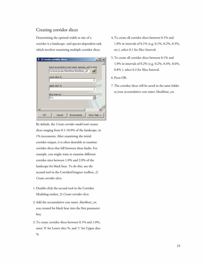
Creating corridor slices

Determining the optimal width or size of a

corridor is a landscape- and species-dependent task

which involves examining multiple corridor slices.

By default, the Create corridor model tool creates

slices ranging from 0.1-10.0% of the landscape, in

1% increments. After examining the initial

corridor output, it is often desirable to examine

corridor slices that fall between these faults. For

example, you might want to examine different

corridor sizes between 1.0% and 2.0% of the

landscape for black bear. To do this, use the

second tool in the CorridorDesigner toolbox, 2)

Create corridor slices.

1. Double-click the second tool in the Corridor

Modeling toolset, 2) Create corridor slices.

2. Add the accumulative cost raster, blackbear_cst,

you created for black bear into the first parameter

box.

3. To create corridor slices between 0.1% and 1.0%,

enter ‘0’ for Lower slice %, and ‘1’ for Upper slice

%

4. To create all corridor slices between 0.1% and

1.0% in intervals of 0.1% (e.g. 0.1%, 0.2%, 0.3%,

etc.), select 0.1 for Slice Interval.

5. To create all corridor slices between 0.1% and

1.0% in intervals of 0.2% (e.g. 0.2%, 0.4%, 0.6%,

0.8% ), select 0.2 for Slice Interval.

6. Press OK.

7. The corridor slices will be saved in the same folder

as your accumulative cost raster, blackbear_cst.

24

GUIDE TO CORRIDORDESIGNER OUTPUT While you choose file names for the major output resulting from the general CorridorDesigner

toolbox, several files are also created automatically.

TEXT LOG FILES

9_10_2007_2215_ ClipAnalysisLayers.txt

(text file)

Log file created by every CorridorDesigner tool.

mo_day_year_hour_toolname.txt

LAYER PREPARATION

Tpi

(raster)

Topographic position index (TPI) created by Create topographic

position raster tool. If the option to delete TPI layer is

unchecked, it will be saved in the same folder as the topographic

position raster. The topographic position index is calculated by

subtracting the focal pixel’s elevation from the average elevation

in a neighborhood surrounding the pixel. For example, a TPI

value of -6 m indicates a focal pixel is 6 m less than the average

elevation in the neighborhood surrounding the pixel. A TPI

value of 14 m indicates the focal pixel has an elevation 14 m

higher than the average elevation of the surrounding

neighborhood.

HABITAT MODELING

[factor]_r

(raster)

Reclassified habitat factors created by Create habitat suitability

model tool. If the option to delete reclassified habitat factors is

unchecked, they will be saved in the same folder as the species’

habitat model. These reclassified habitat factors can be input

along with factor weights into the Combine previously reclassified

habitat factors tool to create a new habitat suitability model.

CORRIDOR MODELING

[species]_0_1_percent_corridor.shp

[species]_2_0_percent_corridor.shp

[species]_4_3_percent_corridor.shp

Corridor slices created by Create corridor model or Create corridor

slices tools.

25

(shapefile)

[species]_cst

(raster)

This grid is used to create new corridor slices using the Create

corridor slices tool.

[species]_hsa

(raster)

Averaged habitat suitability model created during patch

modeling.

[species]_block1patches.shp

(shapefile)

Map of habitat patches found completely within wildland block.

[species]_block1start3.shp

[species]_block1start2.shp

(shapefile)

The Create corridor model tool creates maps of habitat patches

found within each wildland block, and uses these as starting and

ending points for the corridor. If these shapefiles have a 3

appended to them, the corridor ran to a population patch in the

wildland block; a 2 denotes breeding patch, and a 1 denotes that

the corridor ran from any available habitat patch within the

wildland block, because no breeding or population patches are

located in the wildland block.