1

CorrelationA statistical technique that describes the

relationship between two or more variablesVariables are usually observed in a natural

environment, with no manipulation by theresearcher

Example: does a relationship exist between aperson’s age and the number of hours theyexercise per day?

Note: This type of research cannot establishpathways of cause-effect.

2) Each person’s pair of scores canbe plotted on a graph called ascatterplot

Scatterplot of Height and Weight

0

50

100

150

200

250

55 60 65 70 75 80

Height (inches)

We

igh

t (p

ou

nd

s)

Scatterplot of Height and Weight

0

50

100

150

200

250

55 60 65 70 75 80

Height (inches)

We

igh

t (p

ou

nd

s)

3) It is useful to draw an “envelope”,or line around the data in order tosee an overall trend in the data

Subject Height Weight1 77 1852 65 1103 60 1004 72 2005 69 135

1) Correlations require atleast 2 scores for eachperson

2

What’s the strength of relationship? (Chap. 6)

Scatterplot of Height and Weight

0

50

100

150

200

250

55 60 65 70 75 80

Height (inches)

Wei

gh

t (p

ou

nd

s)• Generally, “thin” envelopes

are associated with strongcorrelations, while “fat”envelopes are associated withweaker correlations

• Round (circular) envelopesindicate weak or nocorrelations between the twovariables

What is the relationship? (Chap. 7)

• I.e., what equation can one use topredict Y from X (or vice versa)

• Note, different equations are needed topredict in each direction

4’ 1”

How much does the boy weigh?

Characteristics of a Correlation:• Direction: Correlations can be either positive or negative

–In a positive correlation, the values of the two variables move inthe same direction•High scores on x go with high scores on y

–In a negative correlation, the values of the two variables move inthe opposite direction•High scores on x go with low scores on y

Postive Linear Correlation

-

25

50

75

100

125

150

0 50 100

Negative Linear Correlation

-

25

50

75

100

125

150

0 50 100

Y = a + bX

3

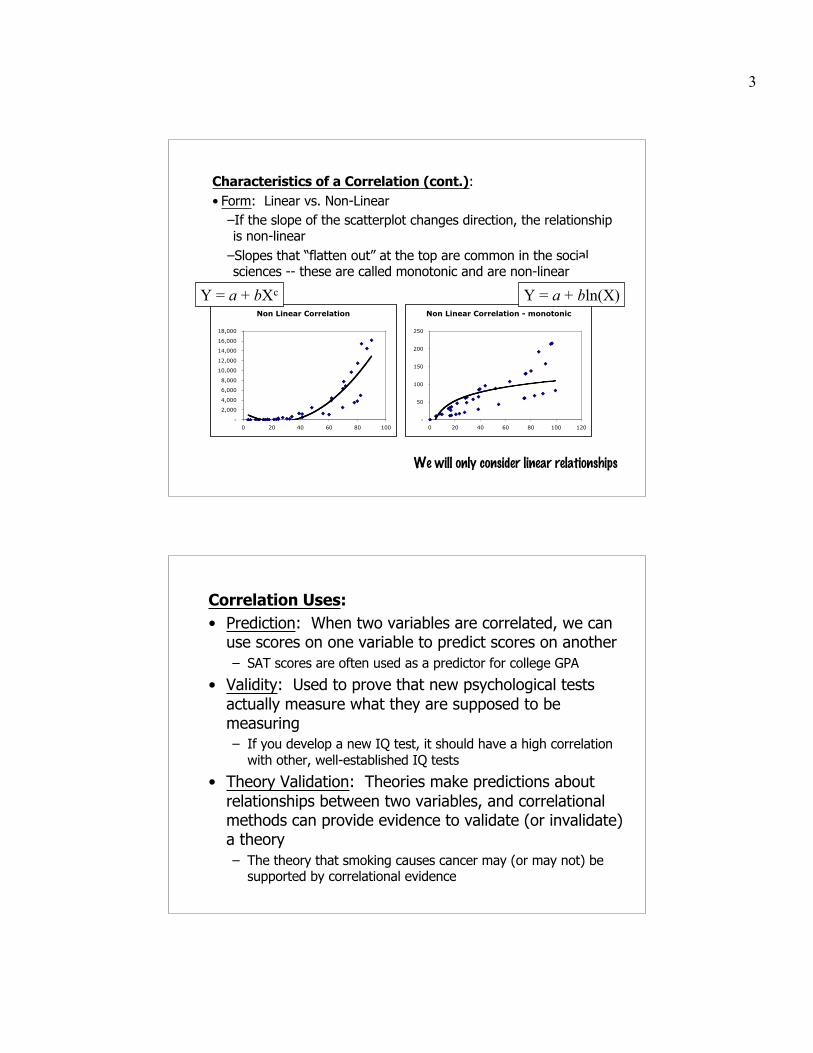
Characteristics of a Correlation (cont.):• Form: Linear vs. Non-Linear

–If the slope of the scatterplot changes direction, the relationshipis non-linear

–Slopes that “flatten out” at the top are common in the socialsciences -- these are called monotonic and are non-linear

Non Linear Correlation

-

2,000

4,000

6,000

8,000

10,000

12,000

14,000

16,000

18,000

0 20 40 60 80 100

Non Linear Correlation - monotonic

-

50

100

150

200

250

0 20 40 60 80 100 120

Y = a + bXc Y = a + bln(X)

We will only consider linear relationships

Correlation Uses:• Prediction: When two variables are correlated, we can

use scores on one variable to predict scores on another– SAT scores are often used as a predictor for college GPA

• Validity: Used to prove that new psychological testsactually measure what they are supposed to bemeasuring– If you develop a new IQ test, it should have a high correlation

with other, well-established IQ tests

• Theory Validation: Theories make predictions aboutrelationships between two variables, and correlationalmethods can provide evidence to validate (or invalidate)a theory– The theory that smoking causes cancer may (or may not) be

supported by correlational evidence

4

• Statistically, the strength and direction of therelationship are expressed by the correlation coefficient(a.k.a. Pearson’s product moment correlation orPearson’s r )

• Correlation coefficients can range in value from -1 to +1– A value of 0 (or near 0) indicates no correlation

– Values of +1.00 or -1.00 are perfect correlations

PEARSON’S CORRELATION COEFFICIENT:• Measures the degree of linear relationship between two

variables

separatelyy vary & which x todegree

ethery vary tog & which x todegree=r

• Another way to phrase the strength-of-relationshipquestion is:How well does the standard score (z-score) ofone variable predict the standard score (z-score)of the other?– Does knowing the number of s.d.’s above or below the

mean one variable is tell us how many s.d.’s above themean the other variable is?

– This phrasing makes it meaningful to relate measureson different scales (e.g., height and weight) or ofdifferent values on the same scale (e.g., heights ofchildren and parents)

• We want a scale that runs from +1 to –1– Perfect positive to perfect negative linear relation

5

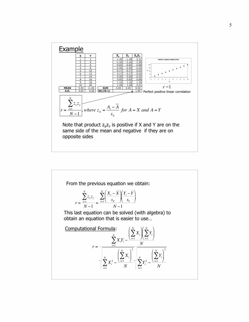
X Y1 22 43 64 85 106 127 148 169 1810 20

MEAN 5.50 11.00 S.D. 3.03 6.06

Zx ZY ZxZY-1.49 -1.49 2.21-1.16 -1.16 1.34-0.83 -0.83 0.68-0.50 -0.50 0.25-0.17 -0.17 0.030.17 0.17 0.030.50 0.50 0.250.83 0.83 0.681.16 1.16 1.341.49 1.49 2.21

SUM 0.00 0.00 9.00SS/(N-1) 1.00

€

r =

zxzyi=1

N

∑N −1

, where zA =Ai − AsA

for A = X and A =Y

PERFECT LINEAR CORRELATION

0

5

10

15

20

0 1 2 3 4 5 6 7 8 9 10

X

Y

Note that product zXzY is positive if X and Y are on thesame side of the mean and negative if they are onopposite sides

r =1Perfect positive linear correlation

Example

From the previous equation we obtain:

Computational Formula: €

r =

zxzyi=1

N

∑N −1

=

Xi − XsX

Yi −YsY

i=1

N

∑N −1

This last equation can be solved (with algebra) toobtain an equation that is easier to use…

€

r =

XiYi −Xi

i=1

N

∑

Yi

i=1

N

∑

Ni=1

N

∑

Xi2 −

Xii=1

N

∑

2

Ni=1

N

∑ Yi2 −

Yii=1

N

∑

2

Ni=1

N

∑

6

X Y1 22 43 64 85 106 127 148 169 1810 20

MEAN 5.50 11.00 S.D. 3.03 6.06

X Y X2 Y2 XY1 2 1 4 22 4 4 16 83 6 9 36 184 8 16 64 325 10 25 100 506 12 36 144 727 14 49 196 988 16 64 256 1289 18 81 324 16210 20 100 400 200

SUM 55 110 385 1540 770

Let’s see how easier..

€

r =

XiYi −Xi

i=1

N

∑

Yi

i=1

N

∑

Ni=1

N

∑

Xi2 −

Xii=1

N

∑

2

Ni=1

N

∑ Yi2 −

Yii=1

N

∑

2

Ni=1

N

∑

=770 − 55( ) 110( )

10

385 − 552

101540 − 110

2

10

=165

82.5( ) 330( )=1

• In the absence of any knowledge of X, onecan do no better than use as the bestguess for Y

• When X and Y are linearly related, thenY’= a+bX gives a better predicted value

• Note the following:€

Y

€

Yi −Y = Yi −Y '( ) + Y '−Y( )

0

10

20

30

40

0 5 10 15

€

Y '−Y

€

Yi −Y '

€

Yi −Y

7

€

Yi −Y = Yi −Y '( ) + Y '−Y( )We solve this equation using more algebra…

€

Yi −Y( )2

∑ = Yi −Y '( )2∑ + Y '−Y( )2

∑

Stays fixed Gets smaller as prediction improvesGets larger as prediction

improves

Total variability of Y (sumof squared deviations of Y

about its mean)

Total variability of Yaccounted for by X (sumof squared deviations of

Y’ about its mean)

Sum of squared deviations ofpredicted from actual Y scores

€

r2 =Y '−Y( )

2∑

Yi −Y( )2∑Coefficient of determination:

€

r2 =Y '−Y( )

2∑

Yi −Y( )2∑

COEFFICIENT OF DETERMINATION:

•The squared correlation value (r2)•Measures the proportion of variabilityin one variable that can be predicted or explained by theother variable -- how much common, or shared, variabilitythe 2 variables have•Example: The correlation between height and weight isr=.89; thus, r2=.79 -- 79% of the variability in the weightscores can be explained or predicted from the heightscores; 79% of the total variability is shared by height andweight

8

Factors affecting Correlations• Restriction of Range: occurs when the Pearson’s r is

calculated from a set of scores that does notrepresent the variable’s full range of values– If only the highest height scores were used to compute the

correlation. Notice how the envelope around those scores isvery circular, indicating a low correlation

Restriction of Range Example

0

50

100

150

200

250

55 60 65 70 75 80Height

Wei

ght

Factors affecting Correlations

• Outliers: The presence of a few extreme scores (outliers)can have an effect on the value of the correlationcoefficient; as indicated by the dashed line, the envelopeis more circular, or wider, indicating a lower correlation

Outlier Example

0

50

100

150

200

250

55 60 65 70 75 80Height

Wei

gh

t

9

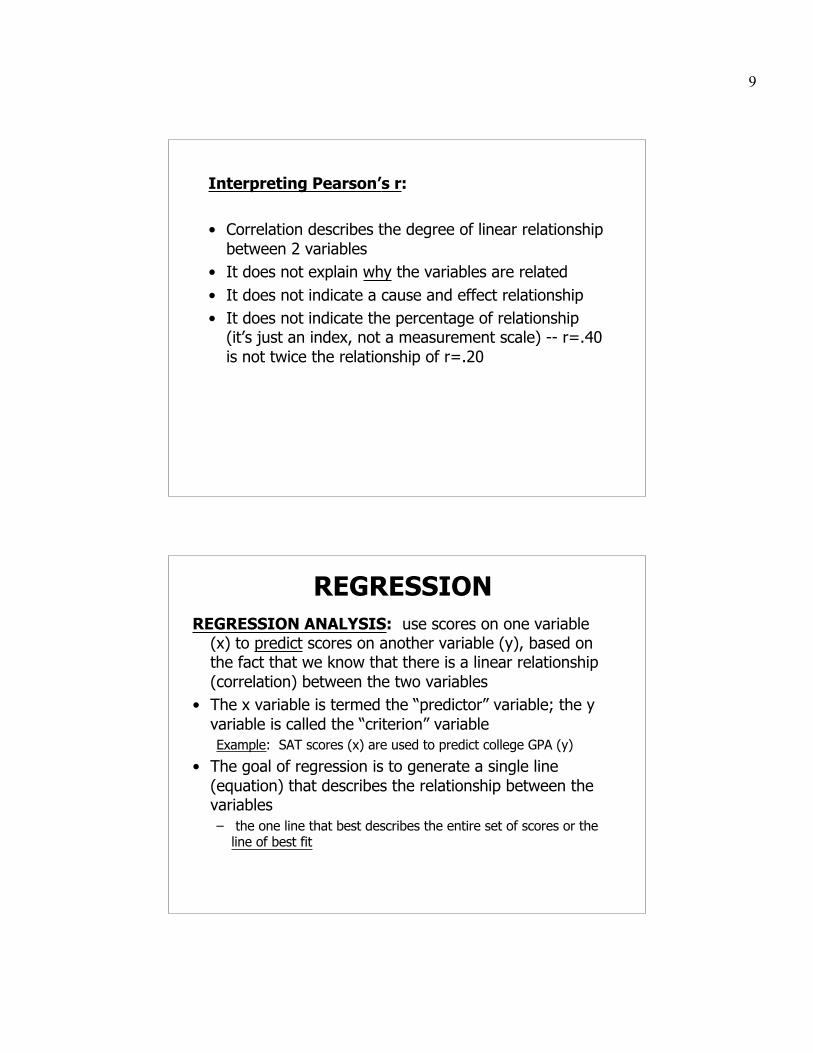
Interpreting Pearson’s r:

• Correlation describes the degree of linear relationshipbetween 2 variables

• It does not explain why the variables are related• It does not indicate a cause and effect relationship• It does not indicate the percentage of relationship

(it’s just an index, not a measurement scale) -- r=.40is not twice the relationship of r=.20

REGRESSIONREGRESSION ANALYSIS: use scores on one variable

(x) to predict scores on another variable (y), based onthe fact that we know that there is a linear relationship(correlation) between the two variables

• The x variable is termed the “predictor” variable; the yvariable is called the “criterion” variableExample: SAT scores (x) are used to predict college GPA (y)

• The goal of regression is to generate a single line(equation) that describes the relationship between thevariables– the one line that best describes the entire set of scores or the

line of best fit

10

Scatterplot of Height and Weight

0

50

100

150

200

250

55 60 65 70 75 80

Height (inches)

Weig

ht

(po

un

ds)

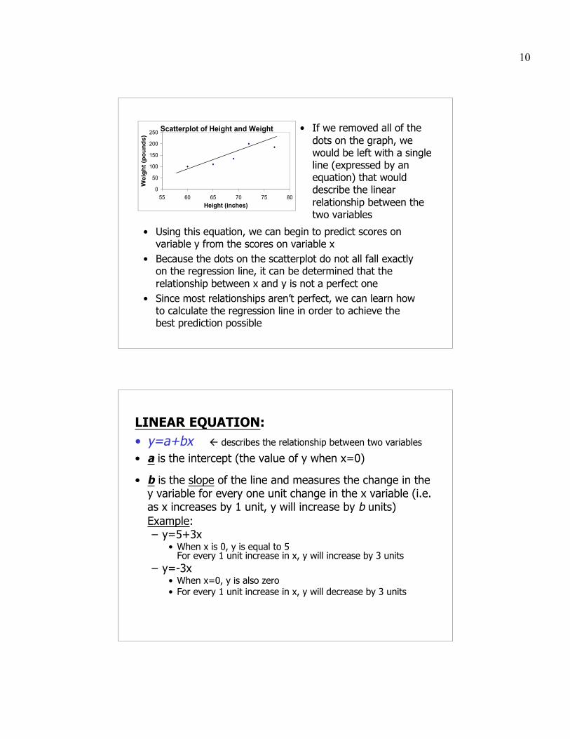
• Using this equation, we can begin to predict scores onvariable y from the scores on variable x

• Because the dots on the scatterplot do not all fall exactlyon the regression line, it can be determined that therelationship between x and y is not a perfect one

• Since most relationships aren’t perfect, we can learn howto calculate the regression line in order to achieve thebest prediction possible

• If we removed all of thedots on the graph, wewould be left with a singleline (expressed by anequation) that woulddescribe the linearrelationship between thetwo variables

LINEAR EQUATION:• y=a+bx describes the relationship between two variables

• a is the intercept (the value of y when x=0)

• b is the slope of the line and measures the change in they variable for every one unit change in the x variable (i.e.as x increases by 1 unit, y will increase by b units)Example:– y=5+3x

• When x is 0, y is equal to 5For every 1 unit increase in x, y will increase by 3 units

– y=-3x• When x=0, y is also zero• For every 1 unit increase in x, y will decrease by 3 units

11

How does one find the “best” straight linewhen the data are not perfect?• We define the best line as the one that minimizes the

sum of squared deviations between observed andpredicted values of Y

• To distinguish observed from predicted write theequations as– Y= a+ bX (observed)– Y’= aY+ bYX (predicted)

• We want to find constants, aY and bY that minimize

€

Yi −Y '( )2i=1

N

∑

0

10

20

30

40

0 5 10 15

Y’ predicted

Y observed

• Consider the expression

• Substitute Y’ for the equation of a straight line,y’=ay+byx, to obtain

• When calculus is used to find the optimal a and b, theresults are

€

Yi −Y '( )2i=1

N

∑

€

Yi − ay +byXi( )( )2

i=1

N

∑

Note, that different equationsare used to predict X from Ythan to predict Y from X

Thus, aY and bY are used toclarify that these are theconstants in the equation usedto predict Y

)(xbya −=

€

yb =xy −

x∑( ) y∑( )n∑

x 2 −x∑( )2n∑

€

y

12

Hints:• If you compare the slope formula to that for Pearson’s r, you will

notice that both the numerator and denominator of this formulaalso appear in the Pearson’s r formula (which will probablyalready have been calculated by the time you reach this step).Don’t recalculate these values, just pull the values from thePearson’s r calculations

• You must first calculate the slope (b) before calculating the y-intercept (a)

• It is risky to predict for values of Xfar beyond those observed

€

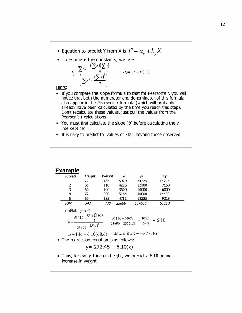
Y '= ay +byX• Equation to predict Y from X is

• To estimate the constants, we use

)(xbya −=

€

yb =xy −

x∑( ) y∑( )n∑

x 2 −x∑( )2n∑

€

y

Subject Height Weight x2 y2 xy1 77 185 5929 34225 142452 65 110 4225 12100 71503 60 100 3600 10000 60004 72 200 5184 40000 144005 69 135 4761 18225 9315

SUM 343 730 23699 114550 51110

x=68.6, y=146( )( )

( )5

34323699

5

73034351110

2

−

−=b 8.2352923699

5007851110

−

−=

2.169

1032= 10.6=

)6.68(10.6146 −=a 46.418146 −= 46.272−=• The regression equation is as follows:

y=-272.46 + 6.10(x)

• Thus, for every 1 inch in height, we predict a 6.10 poundincrease in weight

Example

13

Regression Line Properties:• For every x value, we can generate a predicted y value on

the regression line -- simply plug a given x value into theregression equation

• These predicted y values are designated (y hat)

Example: The predicted weight for someone who is 60inches tall is:

Prediction Error:• For every value of x, we will predict a new y value based

on the regression equation. There will be some distancebetween the actual y value and the new predicted y value

• To determine how well a regression line fits the data, weneed to measure the difference between each actual yvalue and the corresponding predicted y value

y

€

ˆ y = −272.46 + 6.10(60) = 93.54

Example:– Our predicted value is 93.54– The actual weight (y value) for someone who is 60 inches tall is

100 pounds– The difference (6.46) is prediction error

• Prediction error can be visually represented by measuringthe vertical distance between the actual y data point andthe predicted point on the line

• Conceptually, if weadded up all of theseerror values, we wouldget a measure of totalprediction error

• The regression line generated by the equation is the oneline that minimizes the total prediction error thus the term“line of best fit”

yy ˆ−

y

Actual Score

PredictionError

Predicted Score

14

STANDARD ERROR OF ESTIMATE:• Provides a measure of the average distance between a

regression line (predicted scores) and the actual data points;provides information about the accuracy of the predictions

• Conceptually similar to standard deviation in the fact that itprovides an average measure of distance

• Found by averaging the distances between actual scores andthe predicted scores ( )

Standard Error Properties:• As the correlation increases (gets closer to 1.00 or -1.00), the

data points are more tightly clustered around the regressionline, resulting in better prediction (less prediction error)

• As the correlation gets smaller (approaches 0), the data pointsare spread further out from the regression line, resulting inpoorer prediction (greater prediction error)

yy ˆ−

SEE =y − ˆ y ( )2∑

n − 2

Predicting X from Y• The constants in the equation to predict Y from X

derive from minimizing the SSD between observed andpredicted Y

• The constants in the equation to predict X from Yderive from minimizing the SSD between observedand predicted X

€

X '= aX + bxY

€

aX = X − bxY

€

bx =XY∑ −

X∑( ) Y∑( )N

Y 2∑( ) −Y∑( )

2

N

0

10

20

30

40

0 5 10 15

15

Interpreting Regression Analysis:• Regression cannot be used to “extrapolate” values

that fall outside of the range of our actual data pointvalues; we cannot predict extreme scores that fallbeyond the range of our actual scores

Example: Using our previously determined regressionequation, y=6.10x-272.46, predict the weight forsomeone who is 40 inches tall

= 244-272.46 * This leaves us with = -28.46 a negative weight

46.272)40(10.6ˆ −=y