Dynamic Regressions with Variables Observed at Different Frequencies

Tilak Abeysinghe and Anthony S. Tay

Department of Economics National University of Singapore

10 Kent Ridge Crescent Singapore 119260

January 2000

Abstract: We consider the problem of formulating and estimating dynamic

regression models with variables observed at different frequencies. The strategy

adopted is to define the dynamics of the model in terms of the highest available

frequency, and to apply certain lag polynomials to transform the dynamics so that

the model is expressed solely in terms of observed variables. A general solution

is provided for models with monthly and quarterly observations. We also show

how the methods can be extended to models with quarterly and annual

observations, and models combining monthly and annual observations.

Key Words: Variables of different frequencies, dynamic regressions, temporal aggregation, systematic sampling, lag polynomials, serial correlation.

JEL Classification: C22

------------------------ Correspondence to: Tilak Abeysinghe, Department of Economics, National University of Singapore, 10 Kent Ridge Crescent, Singapore 119260. Email: TilakAbey@nus.edu.sg, Ph. (65) 874 6116, Fax. (65) 775 2646.

* The authors would like to thank the NUS Econometrics Reading Group for their

valuable comments.

2

1. Introduction

Economic data are available in a variety of frequencies. Econometric models, on the

other hand, are typically constructed for use with data observed at the same frequencies.

Datasets for use in any one econometric application are thus assembled at the frequency of the

lowest frequency variable, with the data series available at higher frequencies converted to the

lower frequency through temporal aggregation or systematic sampling, depending on whether the

corresponding variables are flow or stock variables respectively. A researcher may, for instance,

be interested in modeling the relationship between output and employment: if output is observed

quarterly and employment monthly, a model incorporating these two variables would have to be

specified at a quarterly frequency, with quarterly employment figures systematically sampled

from the monthly figures.

This paper develops a modeling strategy that avoids the need for all data series within an

econometric application to be sampled at the same time intervals. Dynamic regression models

are formulated which include variables observed at different frequencies. There are clear

advantages to such a modeling approach. Consider the case where the dependent variable is

available quarterly while the independent variable is observed monthly. By allowing the

independent variable to be included in the model at the higher frequency, monthly multipliers

would be available that would otherwise be lost had the monthly data been converted into

quarterly observations. The model would permit updating of quarterly forecasts as monthly data

becomes available. Including monthly dynamics may also improve one-quarter ahead forecasts.

A long history of papers has discussed the effects of systematic sampling and temporal

aggregation on model structure, parameter estimates, forecasting and causal relationships

(Zellner 1966, Brewer 1973, Wei 1981, Weiss 1984, among others), but these works focus on

3

situations where all the variables in the model are available at one frequency whereas the

theoretical model of interest is defined at a higher frequency. Our aim is to develop a way of

including variables at their highest frequencies available, even if these frequencies are not the

same across all variables. The strategy adopted in this paper is that of Abeysinghe (1998, 1999),

which is to define an autoregressive distributed lag model with the dynamics of the model

defined in terms of the highest frequency available among the variables. The problem then is

one of missing observations, and our solution is to apply certain lag polynomials to transform the

dynamics so that the model is expressed solely in terms of the observed variables. Abeysinghe

(1998, 1999) considered a simple model with an AR(1) structure, with the dependent variable

sampled less frequently than the independent variable. Our contribution in this paper is to

provide a solution for the general AR(p) case for models combining monthly and quarterly,

quarterly and annual, and monthly and annual observations. We also indicate how these results

can be extended to other combinations of frequencies.

We begin by introducing the dynamic models that we consider in this paper. Focusing on

the case where the model contains monthly and quarterly data, we show how a straightforward

application of lag polynomials can transform the dynamic model so that only observed

frequencies appear. The coefficients of these lag polynomials are simple functions of the

autoregressive parameters in the original model. Estimation and testing issues are discussed.

Section 3 extends the method to quarterly-annual and monthly-annual combinations, and we

conclude in section 4.

4

2. The Basic Model

The basic autoregressive distributed lag model that we consider is

(1)

where pp LLLL φ++φ+φ+=φ ...1)( 2

21 , rr LLLL β++β+β+β=β ...)( 2

210 . We refer to this as

ARX(p,r) model. The variables xt and yt are assumed to be available at different frequencies, and

the time subscript t is defined in terms of the highest frequency. For example, if xt is monthly

and yt is quarterly then t=1,2,…,T would represent months. The model can include more than

one regressor though for expositional purposes we will stay with just one regressor. Our

approach can also be extended to the ARMAX class of models, but we leave out the MA

structures to keep the exposition clear. In all our examples we will assume that it is the

dependent variable that is observed with the lower frequency, though our results can easily be

adapted for the reverse case.

If the lower frequency variable yt represents a stock variable, and xt is observed at m

times the frequency of yt , then only every mth observation of yt is available, and the observed

data set would comprise },...,,{ 21 Txxx and },...,,{ 2 Tmm yyy where we have assumed for

notational simplicity that the first available observation of yt is at t = m and that T is a multiple

of m. In the quarterly-monthly case, m = 3. If, on the other hand, yt represents a flow variable,

then what is observed of y at every mth period is an aggregation of m flows recorded at the

higher frequency. The ARX(p,r) can be modified to handle the case of a low-frequency flow

variable by temporally aggregating the variables to obtain

(2)

),0(~,)()( 2σεε+β+α=φ iid xLyL tttt

),0(~,)...1()()( 212 σεε+++++β+α=φ − iid LLLXLYL ttm

tt

5

where tm

t yLLLY )...1( 12 −++++= and tm

t xLLLX )...1( 12 −++++= , and the lag polynomials

)(Lφ and )(Lβ are as previously defined. Again, under our assumptions, what is observed of Yt

are the values at m, 2m,…, T whereas Xt is available at all lags.

As the methods we propose are similar for both the stock as well as the flow variable

cases, we will focus on the case where the low frequency variable is a stock variable, and refer to

the flow variable case only when differences arise. Note that in the usual way of dealing with

mismatched frequencies, the higher frequency data is systematically sampled, or temporally

aggregated depending on whether the variable is a stock or a flow. In our framework, whether or

not the higher frequency (independent) variable is aggregated depends on whether the low

frequency (dependent) variable is a flow or a stock. The nature of the higher frequency data is

inconsequential.

2.1 Monthly-Quarterly Data

Consider first the simple case with an ARX(1,r) structure

(3)

where tx (t=1,2,…,T) is observed at monthly intervals whereas ty is observed only quarterly, so

only every third observation of yt is available, i.e., the observed values of yt comprise

}.,...,,{ 63 Tyyy The strategy adopted in Abeysinghe (1998) is to transform the model so that

only the observed frequencies appear. This involves multiplying both sides of (3) by a lag

polynomial )1()1()( 22221 LLLLL φ+φ−=λ+λ+=λ which will convert the model to1

(4)

1 Note that Abeysinghe (1998) adopted a fractional time subscript which we do not follow here.

ttt xLLLyL ν+φ+φ−β+αφ+φ−=φ+ )1)(()1()1( 22233

xLyL ttt ε+β+α=φ+ )()1(

6

to be estimated over τ= 3t , 3/,...,2,1 T=τ . We will refer to the lag polynomial )(Lλ as the

transformation polynomial, and the lower frequency as the observed frequency. In this case, the

transformed error term tt Lv ελ= )( still maintains the iid property at the observed frequency, and

(4) can be estimated by a non-linear LS technique. One of the advantages of this approach is that

although yt is quarterly, the monthly multipliers or impulse responses can easily be worked out

from (4) using )()( 1 LL βφ − once the parameters have been estimated.

In the general ARX(p,r) case the necessary transformation polynomial will be a lag

polynomial of order 2p, )...1()( 22

221

pp LLLL λ++λ+λ+=λ . Applying this transformation to

(1) gives

(5)

where tt Lv ελ= )( . Note that the polynomial )()()( LLL φλ=π is of order 3p. Setting the

coefficients of the unobserved lags of this polynomial to zero, i.e., 02313 =π=π −− jj , j = 1, 2,…,

p, will provide 2p relationships from which we can solve for the 2p coefficients of )(Lλ in terms

of the φ ’s.

For illustration, consider the ARX(2,r) case where )1()( 221 LLL φ+φ+=φ . Multiplying

this polynomial with the transformation polynomial )(Lλ of order 4 will give us the following

lag polynomial of order 6:

642

53241

422314

312213

2211211

)()(

)()()(1

LLL

LLL

λφ+λφ+λφ+λφ+λφ+λ+

λφ+λφ+λ+φ+λφ+λ+φ+λ+

Setting the coefficients of lags 1, 2, 4 and 5 to zero and solving for the λ ’s will yield the

following solution

ttt vxLLyLL +βλ+αλ=φλ )()()1()()(

7

.

,

,

,

224

213

2212

11

φ=λ

φφ−=λφ−φ=λ

φ−=λ

Thus the ARX(2,r) model ttt xLyLL ε+β+α=φ+φ+ )()1( 221 can be expressed in observed

frequencies as

(6)

where 44

33

2211)( LLLLL λ+λ+λ+λ+=λ with the λ ’s as defined above.

The following theorem provides the general solution to the problem of finding the

coefficients of the lag transformation polynomial =λ )L( )...1( 22

221

pp LLL λ++λ+λ+ for the

ARX(p,r) case.

Theorem 1: Let 10 =φ and 0... 221 =φ==φ=φ ++ ppp . If

∑=

−φφ−=λi

jjijjii c

0,2

1 , i = 0, 1, 2, …, 2p,

where

=

−

−=otherwise

jiremif

c ji

1

03

22

, ,

then )...1()...1)(...1( 33

221

22

221

221

pp

pp

pp LLLLLLLLL π++π+π+=λ++λ+λ+φ++φ+φ+

where 0=πk if k = 3j – 1 or 3j – 2 for some j = 1, 2, …, p.

Proof: See Appendix A1.

ttt LxLLyLL ελ+βλ+αλ=φ+φφ−φ+ )()()()1())3(1( 632

321

31

8

The term

−

3

2 jirem refers to the remainder of quotient

3

2 ji −, i.e., we have 2, −=jic

if the difference between the subscripts of jφ and ji−φ is divisible by 3, and 1 otherwise. For

convenience, the coefficients of λ(L) for the AR(1) through to the AR(5) case are tabulated in

Appendix A2.

The case where ty contains a unit root (at the higher frequency) can easily be handled. A

process with a unit root at the higher frequency will display a unit root at the lower frequency

after application of the transformation polynomials. In the quarterly-monthly ARX(2,r) case,

this can be verified by simply substituting 12 1 φ−−=φ into the AR polynomial in (6) and setting

1=L . The unit root ARX(p,r) case can be handled by factoring L−1 out of the p-order AR

polynomial in (1), and applying the transformation for the ARX(p–1) case followed by the

transformation for ARX(1) with 11 −=φ . We illustrate this procedure in the quarterly-monthly

ARX(3,r) case with a unit root. Let )1)(1()( 221 LLLL −φ+φ+=φ . Multiplying this polynomial

with the transformation polynomial )(Lλ′ of order 4 as in the ARX(2,r) case will give us the

following lag polynomial:

(7)

Multiplying (7) by )1()( 2LLL ++=λ ′′ gives

(8)

where tt XxL =λ )(" is a moving sum of xt.

The formulation in (8) is suitable for the situation where xt is a stationary variable. For

example, tyL )1( 3− may be the quarterly inflation rate and xt the monthly unemployment rate. If

ttt LxLLyLLL ελ′+βλ′+αλ′=−φ+φφ−φ+ )()()()1()1)()3(1( 632

321

31

ttt LLxLLLyLLL ελ ′′λ′+λ ′′βλ′+αλ ′′λ′=−φ+φφ−φ+ )()()()()()1()1()1)()3(1( 3632

321

31

9

xt is also a unit root process but not cointegrated with yt, the (1 – L) operator must be applied

throughout equation (7) and as a result txLL )1)((" −λ reduces to txL )1( 3− , and tL ε− )1(

becomes the white noise process. In this case modeling is done using the quarterly differences of

both yt and xt. If yt and xt are I(1) processes and cointegrated, then the model reverts back to the

original form (6) and can be estimated in level form without imposing the cointegrating

restriction. Being a dynamic model, standard t tests apply (Sims et al., 1990).

2.2 Estimation and the Autocorrelation Problem

We have noted in the quarterly-monthly ARX(1,r) stock variable case that the

transformed error process tt Lv ελ= )( is not serially correlated at the observed lags. Estimation

of the model parameters can therefore be carried out using a non-linear least squares method.

However, the transformed errors will be autocorrelated in the general quarterly-monthly

ARX(p,r) flow variable case for 1≥p as well as the quarterly-monthly ARX(p,r) stock variable

case for 2≥p . In the stock variable case, )(Lλ is of order 2p and therefore tt Lv ελ= )(

systematically sampled at every 3rd observation will be an MA(q) process where ]3/2int[ pq ≤

where int[.] is the integer operator (Brewer, 1973). For the flow variable case,

tt LLLv ε++λ= )1)(( 2 and so will follow an MA(q) process with ]3/)1(2int[ +≤ pq .

To get a feel for the size of the autocorrelations involved we explore some simple cases

below. For a general MA( q~ ) process tq

qt LLv εθ++θ+= )...1(~

~1 systematically sampled at

every m periods, the jth autocorrelation at the observed frequency, mjρ , can be computed as

0γγ

=ρ mjmj where 1,)( 0

~

0

2 =θθθσ=εε=γ ∑−

=+− E

mjq

imjiimjttmj , j = 0, 1, 2, …, int[ q~ /m]. In the

10

quarterly-monthly ARX(1,r) flow variable case, the transformed errors tt LLLv ε++λ= )1)(( 2

will follow an MA(1) process at the observed frequency. After substituting for the original AR

parameters, the observed frequency-first order autocorrelation of tv is

41

31

211

211

1 34543

)1(

φ+φ−φ+φ−φ−φ−

=ρm

Figure 1 plots this autocorrelation for stationary values of 1φ . The autocorrelation problem

appears to be small; for values of )0,1(1 −∈φ , which is the more likely region for economic data

(recall that our AR coefficients have signs that are the reverse of the conventional specification),

1mρ is less than 0.21. Unfortunately, there is no reason to expect the autocorrelation problem to

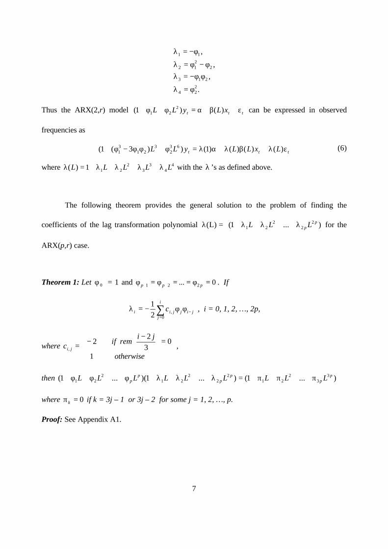
be small for the other cases. Figure 2 plots the first autocorrelation of tt Lv ελ= )( for the

quarterly-monthly ARX(2,r) stock variable case, which also follows an MA(1) process when

systematically sampled at the observed frequency. The autocorrelation is seen to lie between

5.0− and 0.5 for values of 1φ and 2φ in the stationary range. A plot of 1mρ in the ARX(2,r)

flow variable case shows this autocorrelation to range from about 6.0− to 6.0 .

The major obstacle posed by the autocorrelation problem is the inconsistency of the non-

linear LS estimator of the transformed model. Since the autocorrelations, and therefore the MA

parameters, depend on the AR parameters a simple alternative to least squares is to use a non-

linear IV estimator. After computing the autocorrelations from the estimated φ’s, the MA

parameters can be derived by solving the set of non-linear equations given in Box et al. (1994, p.

202, eq. 6.3.1). The same procedure can be used to estimate )var(2tε=σ and the standard errors

of the IV estimator can be recomputed by replacing 2vσ by 2σ (note that 22

vσ≤σ ). One has to

go through the trouble of deriving the MA parameters only if the model is designed for

11

forecasting. If the objective is to derive the impulse responses, then the MA parameters do not

enter the calculations and can be ignored.

The success of the IV estimator depends on the quality of the instrument used. One

possibility is to use lagged dependent variables yt-(p+j), j=1,2,.. as instruments, although this may

not work well if p is large. Monte Carlo studies carried out in relation to a flow ARX(1,1) model

shows that in small samples the LS and IV bias could be similar and may be negligible if the

autocorrelation is small (Abeysinghe, 1999).

Another practical problem is the choice of the lag orders p and r. As observed in

Abeysinghe (1998) if p is known the choice of r is not difficult. Starting with a large value for r

one can test downward to choose an appropriate value for r. Complications arise in the choice of

p because the form of the transformation polynomial )(Lλ depends on p. One possibility is to

treat (5) as a reduced form and estimate it as a linear model. The number of significant lags

would indicate the appropriate order of the lag polynomial )(Lφ . If, for instance, the coefficient

on 6−ty is significantly different from zero while those of 9−ty , 12−ty , …are not, this would imply

p = 2. If r* lags of tx are significant, this would suggest r = r* – 2p (inclusion of 6−ty would

necessarily imply the inclusion of at least four lags of tx ). The disadvantage of this approach is

that some reduced form parameters might be very small, even if the original structural

parameters are not, and in small samples these parameter estimates may turn out to be

statistically insignificant.

In summary, the practical implementation of our modeling approach might take the

following form: if unit root variables are involved, test for cointegration by converting all high

12

frequency variables to the low frequency available2. If cointegration cannot be rejected, use the

level variables for modeling, otherwise use differenced data. Estimating (5) as a reduced form,

as described in the previous paragraphs, would suggest suitable values of p and r, after which (5)

can be estimated using a non-linear IV technique. We suggest overfitting to see if the chosen p

and r are sufficient. Note that the standard t test is applicable here. If the residuals appear to be

empirically white noise, ignoring the MA structure of the transformed model would probably be

inconsequential, and the estimated model may be put to use. In this case a non-linear LS

estimation of the model might be better as the LS estimator is more efficient than the IV

estimator; if the residuals remain white noise under the LS method, the LS estimates would be

preferable for inference. If residual autocorrelation is present, the MA parameters can be derived

as described earlier in this section. An alternative is to identify an ARMA model for the error

term and estimate them together with the model parameters as in the Box-Jenkins transfer

function noise model approach, i.e., generalize the ARX model to an ARMAX structure.

3. Extensions to Quarterly-Annual and Monthly-Annual Cases

Another empirically important case is where the dependent variable is observed annually

and the independent variable is observed quarterly. The general strategy in this case will be to

apply the transformation given in the following theorem twice. The first transformation will

convert the quarterly lag structure into biannual terms, and the second transformation will

convert the biannual structure into an annual structure.

2 Integration and cointegration are invariant to temporal aggregation and systematic sampling (Marcellino, 1999).

13

Theorem 2: Let

iii φ−=λ )1( , i = 1, 2, …, p,

then )...1()...1)(...1( 22

221

221

221

pp

pp

pp LLLLLLLLL π++π+π+=λ++λ+λ+φ++φ+φ+

where 0=πk if k = 2j – 1 for some j = 1, 2, …, p.

Proof: See appendix A1.

For example, consider the AR(2) case ttt xLyLL ε+β+α=φ+φ+ )()1( 221 . We have to

convert this model to a form in which the lag structure on ty only contains the lags in multiples

of 4. Theorem 2 suggests applying the transformation )1()( 221 LLL φ+φ−=λ once to obtain a

lag structure in multiples of 2 for ty to obtain:

ttt LLxLLLyLL εφ+φ−+φ+φ−β+αφ+φ−=φ+φ−φ+ )1()1)(()1())2(1( 221

22121

422

2212 .

Applying a second transformation ))2(1( 422

2212 LL φ+φ−φ− gives us

t

t

t

LLLL

xLLLL

yLL

εφ+φ−φ+φ−φ−+

φ+φ−φ−φ+φ−β+ωφ+φ−φ−φ+φ−=

φ+φ−φ−φφ+

)1)()2(1(

))2(1)(1())2(1)(1(

))22(1(

221

422

2212

422

2212

221

22

21221

822

422

412

21

A similar idea can be applied to the monthly-annual case: first transform the lag structure on ty

to the bimonthly form (using Theorem 2), followed by a transformation to the biannual form

(using Theorem 1) and finally to the annual form (again using Theorem 2).

As in the monthly-quarterly case, these transformations create a problem of

autocorrelation of the transformed error term; the transformed error term follows an MA process

at the observed frequencies in all cases. For each p, the final transformation matrix will be of

14

order 3p, and the transformed error will follow, at the observed lags, an MA(q) process where

]4/3int[ pq ≤ for the stock variable case and ]4/)1(3int[ +≤ pq for the flow variable case.

Finally, we note that the above transformations can easily be adapted to the case where

the independent variable is observed less frequently than the dependent variable. Now the

transformation polynomial λ(L) has to be worked out in relation to β(L) in (1). To apply the

previous results β(L) can be written as )...1()( **10

rr LLL β++β+β=β where

riii ,...,2,1,/ 0* =ββ=β .

4. Concluding Remarks

This paper has provided a modeling approach which allows variables observed at

different frequencies to be framed within a single model without converting the higher frequency

variable into a lower frequency via systematic sampling or temporal aggregation. This approach

entails a number of advantages3. Firstly, we can recover the impulse responses or multipliers at

the high frequency time units. This information is totally lost if one were to use the standard

systematic sampling or temporal aggregation approach. Secondly, this approach is likely to

provide better forecasts compared to those based on the standard approach. Thirdly, forecast

updating can easily be done as and when the high frequency data become available.

The cases that we cover are mostly suitable for macroeconomic analysis, where data are

usually available in monthly, quarterly or annual frequencies. An extension to other

combinations of frequencies may be fruitful, especially for areas like finance. Other possible

avenues for future research include the extension of our methods to vector autoregression models

and for causality testing.

3 For an illustrative application see Abeysinghe (1998).

15

References

Abeysinghe, T., 1998, Forecasting Singapore’s Quarterly GDP Growth with Monthly External

Trade, International Journal of Forecasting 14, 505-513.

Abeysinghe, T., 1999, Modeling Variables of Different Frequencies, International Journal of

Forecasting, forthcoming.

Box, G.E.P., G.M. Jenkins, and G.C. Reinsel, 1994, Time Series Analysis: Forecasting and

Control, 3rd ed., (Prentice-Hall, Inc., New Jersey).

Brewer, K.R.W., 1973, Some Consequences of Temporal Aggregation and Systematic Sampling

for ARMA and ARMAX Models, Journal of Econometrics 1, 133-154.

Marcellino, M., 1999, Some consequences of temporal aggregation in empirical analysis, Journal

of Business and Economic Statistics 17, 129-136.

Sims, C.A., J.H. Stock, and M.W. Watson, 1990 Inference in Linear Time Series with Some Unit

Roots, Econometrica 58, 113-44.

Wei, W.W.S., 1981, Effect of Systematic Sampling on ARIMA models, Communications in

Statistics: Theory & Methods 10, 2389-2398.

Weiss, A.A., 1984, Systematic Sampling and Temporal Aggregation in Time Series Models,

Journal of Econometrics 26, 271-281.

Zellner, A., 1966, On the Analysis of First Order Autoregressive Models with Incomplete Data,

International Economic Review 7, 72-76.

16

Appendix A1

Proof of Theorem 1

By multiplying )...1)(...1( 22

221

221

pp

pp LLLLLL λ++λ+λ+φ++φ+φ+ , and

substituting the expressions for iλ from the theorem, we see that kπ takes the form

ik

k

ijij

i

jji

k

iikik

c −=

−=

=−

φφφ−=

φλ=π

∑∑

∑

0 0,

0

2

1

where

=

−

−=otherwise

jiremif

c ji

1

03

22

, .

Note that the subscripts of jφ , ji−φ and ik −φ add up to m. Note also that for kπ to be zero, all

terms in the double summation containing the same set of φ ’s must sum to zero, e.g., all terms of

the form, say, 431 φφφ , must sum to zero, likewise all 252 φφ terms must sum to zero, and so on.

Consider any one term in the summation in kπ containing, aφ , bφ and bak −−φ (where aφ ,

bφ and bak −−φ are not necessarily distinct). aφ , bφ and bak −−φ may appear because aj = ,

bji =− and bakik −−=− . There are six possibilities, with the corresponding values for i and

ji 2− , as follows

17

j i – j k – i i i – 2 j

a b k – a – b a + b b – a

a k – a – b b k - b k – 2a – b

b a k - a – b a + b a – b

b k – a – b a k – a k – a – 2b

k – a – b a b k – b 2a + b – k

k – a – b b a k – a 2b + a – k

We now show that 0=πk for each of these 6 cases, when k takes the form 13 −j or

23 −j for any positive integer value j . This amounts to showing that 00 0

, =∑∑= =

k

i

i

jjic in each

case.

For these 6 cases, we have to divide the problem into 18 sub-cases, 9 each for the cases

where k takes the form 13 −j and 23 −j , and depending on whether a takes the form 3m, 3m –

1 or 3m – 2 , and whether b takes the form 3n, 3n – 1 or 3n – 2 , where m and n are arbitrary

integer values. The label the eighteen sub-cases as follows

18

case k a b case k a b

1 3n 10 3n

2 3m 3n – 1 11 3m 3n – 1

3 3n – 2 12 3n – 2

4 3n 13 3n

5 3j – 1 3m – 1 3n – 1 14 3j – 2 3m – 2 3n – 1

6 3n – 2 15 3n – 2

7 3n 16 3n

8 3m – 2 3n – 1 17 3m – 2 3n – 1

9 3n – 2 18 3n – 2

The following table shows jic , for each of the 18 x 6 cases, and computes ∑∑= =

k

i

i

jjic

0 0, for each

case :

case

i – 2j 1 2 3 4 5 6 7 8 9 10 11 12 13 14 15 16 17 18

b – a -2 1 1 1 -2 1 1 1 -2 -2 1 1 1 -2 1 1 1 -2

k – 2a – b 1 -2 1 1 1 -2 -2 1 1 1 1 -2 -2 1 1 1 -2 1

a – b -2 1 1 1 -2 1 1 1 -2 -2 1 1 1 -2 1 1 1 -2

k – a – 2b 1 1 -2 -2 1 1 1 -2 1 1 -2 1 1 1 -2 -2 1 1

2a + b – k 1 -2 1 1 1 -2 -2 1 1 1 1 -2 -2 1 1 1 -2 1

2b + a – k 1 1 -2 -2 1 1 1 -2 1 1 -2 1 1 1 -2 -2 1 1

∑∑= =

m

n

n

jjnc

0 0, 0 0 0 0 0 0 0 0 0 0 0 0 0 0 0 0 0 0

19

In all cases 00 0

, =∑∑= =

k

i

i

jjic , hence 0=πk . A similar exercise for k of the form 3j will show that

in that case 0≠πk in general. Q.E.D.

Proof of Theorem 2

By multiplying )...1)(...1( 221

221

pp

pp LLLLLL λ++λ+λ+φ++φ+φ+ , we see that kπ

takes the form,

ik

k

ii

i

k

iikik

−=

=−

φφ−−=

φλ=π

∑

∑

0

0

)1(

for pk ...,,2,1= . If k of the form 2j – 1 then there is an even number of terms in the summation,

with the aka −φφ terms canceling out the aak φφ − terms, therefore 0=πk if k is odd. Q.E.D.

20

Appendix A2

The following table provides the coefficients of the transformation polynomial )...1( 2

22

21p

p LLL λ++λ+λ+ for the ARX(p,.) case where the dependent variable is observed

quarterly and the independent variable is observed monthly. ji,λ refers to the coefficient in the

ijth cell indicated by row λi and column ARX(j,.).

ARX(1,.) ARX(2,.) ARX(3,.) ARX(4,.) ARX(5,.)

1λ 1φ− 1,1λ 1,1λ 1,1λ 1,1λ

2λ 21φ 21,2 φ−λ 2,2λ 2,2λ 2,2λ

3λ 21φφ− 32,3 2φ+λ 3,3λ 3,3λ

4λ 22φ 312,4 φφ−λ 43,4 φ−λ 4,4λ

5λ 32φφ− 413,5 2 φφ+λ 54,5 φ−λ

6λ 23φ 423,6 φφ−λ 514,6 φφ−λ

7λ 43φφ− 524,7 2 φφ+λ

8λ 24φ 534,8 φφ−λ

9λ 54φφ−

10λ 25φ

21

Figure 1 Autocorrelation in the Quarterly-Monthly Flow Dependent Variable ARX(1,r) Case

-1 -0.5 0 0.5 1-0.1

-0.05

0

0.05

0.1

0.15

0.2

0.25

ρ

φ1

22

Figure 2 Autocorrelation in the Quarterly-Monthly Stock Dependent Variable ARX(2,r) Case

-2 -1.5 -1 -0.5 0 0.5 1 1.5 2-0.5

0

0.5

ρ

φ1

φ2 = 0.9 →

φ2 = 0.5 →

φ2 = 0.2 →

φ2 = -0.5 →

Notes: The dashed portions of the graphs show values of ρ in the non-stationary range of 1φ

and 2φ .