Copyright

by

Sai Krishna Yayavaram

2004

The Dissertation Committee for Sai Krishna Yayavaram certifies that

this is the approved version of the following dissertation:

Structure of a firm’s knowledge base and the

effectiveness of technological search

Committee:

________________________________________ James W. Fredrickson, Co-Supervisor

________________________________________ Gautam Ahuja, Co-Supervisor

________________________________________ George P. Huber

________________________________________ Douglas Morrice

________________________________________ Andrew Henderson

Structure of a firm’s knowledge base and the

effectiveness of technological search

by

Sai Krishna Yayavaram, B.Tech

Dissertation

Presented to the Faculty of the Graduate School of

the University of Texas at Austin

in Partial Fulfillment

of the Requirements

for the Degree of

Doctor of Philosophy

The University of Texas at Austin

August 2004

DEDICATION

To Salila, Siddharth and Arnav

ACKNOWLEDGEMENTS

I would like to thank members of my committee Gautam Ahuja, Jim Fredrickson,

George Huber, Doug Morrice and Andy Henderson for all their comments and

suggestions on my dissertation. Your invaluable advice played a large role in improving

my dissertation. I would especially like to thank Gautam who has devoted considerable

time over the years in being a mentor to me and helped me develop as a researcher.

I would like to thank my wife, Salila, who provided enormous support and

encouragement during all stages of my doctoral work. I would also like to thank my

fellow students from the doctoral program who have helped me in innumerable ways.

v

Structure of a firm’s knowledge base and the effectiveness of technological search

Publication No. ___________

Sai Krishna Yayavaram, Ph.D.

The University of Texas at Austin, 2004

Supervisors: James W. Fredrickson and Gautam Ahuja

This dissertation examines the impact of coupling that exists between the knowledge

elements of a firm (i.e., the structure of the firm’s knowledge base) on the firm’s

technological search activity. I define coupling as the decision made on how the search

across two knowledge elements should be combined and distinguish it from

interdependence, which is the inherent relationship between these two elements. I ask

two questions: 1) How does the structure of a firm’s knowledge base impact the

usefulness of a firm’s inventions? 2) How does the prior structure of a firm’s knowledge

base affect the malleability of the knowledge base? Malleability is defined as the

capacity for adaptive change.

vi

Inventions are generated when existing knowledge elements are combined in novel

ways. Given the large number of potential combinations of knowledge elements, the

problem of searching for technological inventions is computationally intractable. I use

the NK model to study this computationally complex problem and argue that the

structure of a knowledge base can mitigate the negative effects of complexity. In the

first part of the dissertation, I show through computer simulations that a structure that is

nearly decomposable (i.e. high coupling within a cluster of elements along with low

coupling across clusters) increases the effectiveness of search on an NK landscape. In

the second part of the dissertation, I test the relationship between near decomposability

in the structure of a knowledge base and technology search in the context of the

worldwide semiconductor industry. I find support for the hypothesis that a nearly

decomposable structure improves the search for technological inventions. Further, I also

find support for the hypothesis that firms with a nearly decomposable structure are

likely to undergo a larger change in their knowledge base over time.

vii

TABLE OF CONTENTS

GLOSSARY ix

1 INTRODUCTION 1

2 LITERATURE REVIEW 11

3 A SIMULATION BASED STUDY ON THE EFFECT OF COUPLING ON SEARCH ON AN NK LANDSCAPE

56

4 EMPIRICAL HYPOTHESES 67

5 METHODS AND MEASURES 86

6 RESULTS 105

7 CONCLUSIONS AND FUTURE RESEARCH 115

TABLES 125

FIGURES 149

REFERENCES 165

VITA 172

viii

GLOSSARY

System A collection of interacting nodes or elements or

components or very broadly, decisions. Examples: an economy, a strategy, a knowledge base

N Number of nodes in a system

Interdependence The extent to which the value or payoff of one element depends on other elements

K Number of nodes whose states affects a focal node’s value, i.e. the number of nodes with which a focal node is interdependent

State of node i si = 0 or 1

Configuration S = {s1, s2, s3 … sN}

Value contributed by a node ci = ci (si; si1, si2 …siK)

Value of System C(S) = [Σi ci ] / N

Landscape Set of all possible configurations and the value associated with each configuration

J Number of clusters

NJ Number of nodes in a cluster = N/J

Cluster {1,2…NJ} ε Gj, j=1 to J

Cluster value C(Gj) = [Σi ci ] / NJ, i ε Gj

Coupling Decision taken on how the search across two interdependent elements should be combined Lij = the weight given to the state of node j by the decision-maker in deciding the state of node i

Integration Coupling between clusters

Structure L – set of couplings between all elements of the system

Experiential search Trial and error search in which firms make an online evaluation of alternatives and accept those trials that

ix

are successful

Cognitive search Off-line evaluation of alternatives where testing is performed on mental models of the environment

x

1 INTRODUCTION

“The aim of science is not things themselves, …, but the relations among things;

outside these relations there is no reality knowable”

- Henri Poincare in Science and Hypothesis (1905)

1.1 The research questions

In this dissertation, I examine the impact of coupling that exists between the knowledge

elements of a firm on the firm’s technological search activity. The couplings between

the elements of a firm’s knowledge base comprise the structure of its knowledge base. I

define coupling as the decision made on how the search across two knowledge elements

should be combined and distinguish it from interdependence, which is the inherent

relationship between these two elements. I ask two questions: 1) How does the structure

of a firm’s knowledge base impact the usefulness of a firm’s inventions? 2) How does

the prior structure of a firm’s knowledge base affect the malleability of the knowledge

base? Malleability is defined as the capacity for adaptive change.

1.2 Theoretical perspectives and motivation

The knowledge-based view of the firm suggests that the firm’s knowledge base, the

domain of search and the type of search are some of the key determinants of the

effectiveness of technology search (see Figure 1). The domain of search represents the

choice between exploitation and exploration (March, 1991). The two broad types of

1

search considered in this study are experiential search and cognitive search (Gavetti and

Levinthal, 2000). Experiential or trial and error search involves online evaluation of

alternatives and acceptance of those trials that are successful. Cognitive search involves

off-line evaluation of alternatives where testing is performed on mental models of the

environment. Prior literature in this area has mainly conceptualized a firm’s knowledge

as a set of elements or components (Stuart and Podolny, 1996; Ahuja and Lampert,

2001; Fleming, 2001; Katila and Ahuja, 2002). In addition to the elements themselves, a

firm’s knowledge resides in the relationship or coupling between these elements as

well. Considering the structure of these relationships can provide additional insight into

the factors that affect technology search.

The effectiveness of technological research can be measured in two different ways.

One, it can be measured as the usefulness of inventions that are being generated in the

current time period. Second, it can be measured as the usefulness of inventions that are

generated in later time periods. For future inventions to be generated, a firm’s

knowledge base has to change to keep pace with a changing technological environment

and to avoid the exhaustion of useful combinations (Fleming, 2001). This capacity for

adaptive change is termed here as malleability. Technology search in the current time

period (a flow variable) has an important effect on the changes that occur in a

knowledge base (a stock variable). Hence, it is useful to examine the effect of structure

in the current time period on the changes that occur in the knowledge base. Looking at

2

how a knowledge base (and implicitly, its structure) changes also makes it possible to

address the issue of what determines structure. Hence, the two outcomes that are being

studied in this dissertation are the usefulness of inventions generated in the current time

period and the changes that occur in a knowledge base.

The motivation for studying the impact of structure is as follows. A technological

invention can be seen as a recombination of existing knowledge elements (Gilfillan,

1935; Schumpeter, 1939; Fleming, 2001). For example, a new type of storage device

that is being developed by IBM is based on punching holes using a scanning tunneling

microscope which was invented in 1981 and whose initial purpose was to produce

images of single atoms (Chang, 2002). Like computer punch cards, an early form of

computer storage, this new system also stores information in holes, though of a much

smaller size. Thus, recombining one element of knowledge, holes to store data, with

another element, scanning technology, resulted in a new invention.

The large number of potential combinations of existing elements leads to a

combinatorial explosion of the space of possible inventions. For instance, with just 100

elements and considering the simple case of an element being used/ not used, the

number of possible combinations is 2100. The actual number of knowledge elements is a

much larger number. The NK-model has been developed by Kauffman (1993) to study

such computationally complex problems. The two key parameters of the NK model are

N, the number of elements in a system (here, technology) and K, the number of

3

interdependencies between the elements. These two parameters can be used to generate

N-dimensional landscapes that are either smooth or rugged. Useful inventions can be

seen as the peaks on such a landscape. Computational complexity refers to the fact that

it is difficult to locate these peaks on such N-dimensional landscapes. To know how the

search process can be improved, it is necessary to study the effect of the parameters of

the model and the nature (viz. domain and type) of the search process.

A simple example of the elements in a technology (design of a coffee mug1) is shown in

Table 1. Each element can exist in various states. For example, the material of the

coffee mug can be either plastic or ceramic. The interdependencies across these

elements are shown in Table 2. For example, the manufacturing process depends on the

type of material. The goal of technology search is to identify a set of states or a

configuration that results in a coffee mug with certain desirable properties. Mug 1, a

ceramic mug, and Mug 2, a plastic mug, (Table 1) represent the outcomes or the

artifacts generated by this search process.

Prior literature has discussed the effect of interdependence (high vs. low) and the nature

of search (local vs. distant, experiential vs. cognitive) on the effectiveness of search

(Kauffman, 1993; Kauffman et al 2000; Gavetti and Levinthal, 2000). An important

result derived by Kauffman (1993) is that as K (the degree of interdependence)

increases, the landscape becomes more rugged, making it difficult to locate good peaks.

4

1 While this example refers to the design of a product and not a knowledge base, it still provides a useful illustration of the concepts of interdependence and coupling.

This deterioration in the outcomes of the search process as the number of

interdependences in the system increases is termed as the complexity catastrophe

(Kauffman, 1993). I develop an extension of the NK-model by introducing the concept

of coupling and seek to show that coupling has a significant impact on the effectiveness

of search even on landscapes that are rugged.

The concept of coupling can be illustrated as follows2. In designing the coffee mug, the

designer can partition the elements into subsets. A simple way would be to partition the

elements into those related to manufacturing, the vessel and the handle (Table 3). The

design process can be then carried on independently in these three sub-sets; this idea is

captured in the concept of coupling3. In this particular example, the search processes for

the elements in each subset are strongly coupled with each other and the search

processes for elements that are in two different subsets are weakly coupled. The pattern

of these couplings comprises the structure of the knowledge base of the firm.

This example also brings out the differences between interdependence and coupling

(summarized in Table 4). The decision on which elements should be strongly coupled

and which elements should be weakly coupled belongs to the made world – the world of

human designed artifacts. In contrast, interdependence exists in the natural world – the

world of laws of nature. These laws (going by our current knowledge) imply that unlike

plastics, ceramics cannot be injection molded. A second important difference is that

5

2 A formal definition of coupling is provided in §2.3 after the NK model is discussed in more detail. 3 The concept of coupling is closely related to the idea of modularity, as discussed later.

interdependence is often not known a priori. For example, it may be that ceramics can

indeed be injection molded but we do not how to do it as yet. Uncovering such

previously unknown relationships or getting a better understanding of these

relationships is a very important aspect of technology search. I develop arguments on

how coupling plays an important role in uncovering or improving our knowledge of

these interdependencies.

To hypothesize about the desired structure of a knowledge base, I draw upon the

literature on design modularity and the related work on nearly decomposable systems

(Simon, 1962). In particular, I seek to show that an intermediate level of coupling

between clusters of a firm’s knowledge elements achieves the right balance between

exploitation and exploration that is required for effective technology search. Further, I

seek to show that such a structure makes a knowledge base malleable, mainly because it

increases the absorptive capacity of the firm with respect to knowledge generated

through either experiential or cognitive search.

1.3 Research Design

In the first part of this dissertation, I examine the effect of coupling on the effectiveness

of search on NK landscapes through a simulation-based study. These simulations extend

the work done by Kauffman and his colleagues (Kauffman, 1993; Kauffman et al 1994;

Levitan et al, 1999). I also use these simulations to show that the optimal level of

coupling is associated with a balance between exploration and exploitation.

6

In the second part of the dissertation, I use the results from the simulation study to build

hypotheses that are tested empirically in the context of the worldwide semiconductor

industry. Longitudinal data from 1981 to 1999 was used. A number of reasons motivate

the choice of semiconductors as the setting for the study. First, the high R&D intensity

of the semiconductor implies that technology search is of considerable importance in

this industry. Second, use of scientific knowledge is taken as a measure of cognitive

search in this study. As the semiconductor industry has a high reliance on scientific

knowledge (Klevoric et al, 1995), it provides an opportunity to study the effects of

cognitive search.

1.4 Contributions

This dissertation makes a contribution to the literature on complex adaptive systems by

introducing the concept of coupling into the NK model. Prior research, for the most

part, has treated interdependence and coupling as equivalent concepts (or defined

coupling as interdependence across organisms (Kauffman, 1993)). The issue of how

knowledge of interdependencies is accumulated also has not been considered. This

dissertation brings out the difference between the two concepts and goes further by

examining the role of coupling in how interdependencies are discovered. Following

Kauffman (1993), many researchers have argued that interdependencies in a system

should be reduced to avoid the complexity catastrophe. I point out that changing

interdependencies is beyond the control of a decision-maker, especially in the case of

7

technology search. I argue that instead of trying to reduce interdependencies, one should

focus on choosing the appropriate structure of the coupling matrix to mitigate the

effects of the complexity catastrophe. Results from computer simulations show that a

nearly decomposable structure improves the search on NK landscapes, as compared to a

completely decomposed structure or no structure, even when interdependencies are

pervasive.

Second, this study makes a contribution to the literature on modularity by making clear

the mechanisms through which modularity affects technology search. It connects the

literature on modularity (and the associated literature on nearly decomposable systems)

with the NK model. Prior research has mostly assumed that near decomposability exists

in the interdependence matrix. I argue that near decomposability actually exists in the

coupling matrix and show that this near decomposability of the coupling matrix

improves the search process whether or not the interdependence matrix is nearly

decomposable. I develop on Levitan et al’s (1999) idea that complete modularity

achieves the right balance between exploitation and exploration and show that near

decomposability (i.e. modularity combined with integration between modules) has the

same effect. Further, I seek to show that near decomposability in the coupling matrix

makes the knowledge base malleable by increasing the absorptive capacity of the firm

with respect to the knowledge generated through experiential or cognitive search.

8

Third, this study contributes to our understanding about the role of science in

technology search. Prior research has suggested that science provides knowledge of

interdependencies (Fleming and Sorenson, 2001). However, the mechanism through

which such knowledge is used has not been made clear. In this study, I seek to show

that scientific knowledge about interdependencies is mainly used in changing the

structure of the coupling matrix. A more generalized implication that can be drawn from

this study is that the knowledge generated through experiential or cognitive search, in

addition to affecting the elements, affects the structure of the knowledge base as well.

Fourth, this study is a part of a planned research stream that explores the application of

Complex Adaptive Systems (CAS) theory to the fields of management and strategy. In

further work, I intend to apply the concept of coupling to issues such as organization

design, firm scope and intermediation. The idea of near decomposability in the coupling

matrix can be applied to coupling between organizational sub-units (the issue of

organization design) and coupling between firms (the issues of firm scope and

intermediation). In a related paper, I am attempting to show that the concept of coupling

provides an explanation of the effect of Information Technology on firm scope that

improves upon the explanations provided by the traditional theories of the firm. In

further work, I intend to explore the effects of IT on organization design and

intermediation by using the concept of coupling.

9

From an empirical standpoint, this study introduces a new measure of coupling. This

measure also captures the combinative aspects of a firm’s technological competencies.

It is also one of the few studies that test the results from the NK model in an empirical

setting. From the managerial practice point of view, this study seeks to make explicit

the desired structure of a knowledge base that maximizes the effectiveness of

technology search.

10

2 LITERATURE REVIEW

In this section, I review the three streams of literature on which this study is based:

technology search, modularity and the NK model. In the sub-section on technology

search, I explore the key issues that have an impact on the effectiveness of technology

search and discuss how they have been addressed by prior work. One such issue is

modularity, which is discussed extensively in the second sub-section. Finally, I review

the prior work on the NK model, discuss its usefulness in management and strategy and

then focus on how it has been used to study technology search and modularity.

2.1 Technology Search

Technology search is defined as the search for useful inventions. In discussing the

literature on technology search, I will also discuss the broader literature on search

focusing mainly on firm-specific characteristics.

2.1.1 Technology search as problem solving

Technology search is usefully seen as a problem-solving activity (Nelson and Winter,

1982; Ahuja and Katila, 2002). The problem of technology search is to find useful

inventions by searching through a space of possibilities. The space is usually called a

technology landscape as the landscape metaphor is seen as appropriate for the problem

of technology search. The goal of the search process is find hills or local peaks on the

landscape. These local peaks represent inventions.

11

2.1.2 Technology search and bounded rationality

An important aspect of the search process is that it is governed by bounded rationality

(March and Simon, 1958). Bounded rationality has two aspects. One, managers cannot

calculate the optimal solution due to the limits on their cognitive ability. This is the

aspect that has been studied extensively in the literature and has been used to explain

local search. The second aspect of bounded rationality refers to the difficulty in

knowing where the peaks are located on the landscape, not because managers lack the

necessary skills but due to the difficulty in devising formal algorithms and generating

close-ended solutions (Simon, 1996). The topography of the landscape cannot be

determined and the location of the peaks cannot be calculated due to the computational

complexity associated with the combinatorial explosion of the solution space4. Hence

managers have to use heuristics to search for good local peaks on the landscape. The

focus of this study is on this second aspect of bounded rationality.

In this study, I use the NK model (Kauffman, 1993) to explicitly model the

computational complexity that is associated with search on a landscape. While many

implications of complexity such as the presence of multiple optima, necessity of local

search and the presence of path dependence are very much the same as the conclusions

made by the extensive literature on search, the main difference between these two

streams is in what they consider as the drivers of these phenomena. The prior search

12

4 More accurately, it is widely believed but not proven that such combinatorial optimization problems cannot be solved in reasonable time (Rivkin, 2000). Providing a formal proof for this assertion is an important unsolved mathematical problem (http://www.claymath.org/millennium/P_vs_NP/).

literature focuses more on how search is constrained by organizational characteristics

and cognitive limitations of humans whereas the computational complexity perspective

emphasizes how search is constrained by the combinatorial explosion of the solution

space. As such, the complexity perspective focuses on ways in which these constraints

of complexity can be minimized.

2.1.3 The evolutionary nature of technological search

A second important aspect of search is its evolutionary nature. There are a large number

of studies that have explored the evolutionary nature of technology search and

developed a number of key ideas. First, technology search is characterized by path

dependence (Nelson and Winter, 1982). Technology develops on a trajectory (Sahal,

1981; Dosi, 1988) through a series of small improvements. While most of the progress

occurs through small changes (Mokyr, 2002), occasionally a large change occurs due to

a technological discontinuity (Tushman and Anderson, 1986). A second important

aspect of technological search is that it involves recombinant search (Gilfillan, 1935;

Schumpeter, 1939; Fleming, 2001). Most, if not all, inventions are generated when

known elements of knowledge are combined in a novel way. The idea that search is

characterized by path dependence and recombination is present in the computational

complexity perspective also, as discussed in §2.3.

Next, I define effectiveness of technological search and then discuss the determinants of

the effectiveness of technology search (Figure 1). As inventions are recombinations of

13

knowledge elements, the existing knowledge base of the firm is an important

determinant of the effectiveness of technology search. In addition, the domain of search

and the type of search are important determinants as discussed later.

2.1.4 Defining effectiveness of technological search

There are two important measures of the effectiveness of technological search. First,

effectiveness can be measured in terms of the usefulness of inventions generated in the

current time period. Second, effectiveness can be measured in terms of the malleability

of a knowledge base. Broadly speaking, any changes that occur in the knowledge base

of a firm (knowledge stock) would be a result of knowledge generation (knowledge

flows). As shown in Figure 1, the knowledge flows associated with the search process

and the inventions generated in the current time period affect the changes that occur in

the knowledge base of the firm and in turn the inventions generated in the next time

period. If the knowledge base is not malleable (i.e. if it is not capable of undergoing

adaptive change), inventions that are derived from the knowledge base become less

useful over time as the potential for recombination is exhausted (Fleming, 2001; Ahuja

and Katila, 2002). Also, a knowledge base has to be malleable so that the firm can keep

pace with a changing environment. Hence, malleability of the knowledge base is an

additional important measure of the effectiveness of technological search.

14

2.1.5 The constituents of a knowledge-base

The two important constituents of a knowledge base are its elements and its structure.

The elements of the knowledge base specify the position that a firm occupies on the

technology landscape. The position of a firm is usually defined using the firm’s existing

patents (e.g., Jaffe, 1989), its R&D expenditures (e.g., Helfat, 1994) or by its human

resources (e.g., Chang, 1996). As this study also uses inventions in the form of patents

to define a firm’s position, I discuss this method in greater detail. One such method

starts by placing a firm’s inventions in several technology categories, usually patent

classes (Jaffe, 1989, Patel and Pavitt, 1997; Silverman, 1999; Ahuja, 2000). A vector

then gives the position of a firm, with each element in the vector representing the

fraction of the firm’s inventions that fall in that category. Each element in this vector

can be considered as a technological competence (Patel and Pavitt, 1997) or as a

component competence (Henderson and Clark, 1990). Further, each firm’s position can

be additionally specified by its distance from its competitors (Stuart and Podolny, 1996;

Ahuja, 2000) or a technology cluster (Jaffe, 1989).

The focus of this study is on the structure of a firm’s knowledge base, which I argue is

also an important constituent of a firm’s knowledge base. The structure of a knowledge

base refers to the pattern of relationships that exist between the elements. Structure

represents the extent to which the search across pairs of elements is combined or

coupled as discussed further in greater detail in §2.2 and §2.3. Structure also represents

15

the combinative capabilities (Kogut and Zander, 1992) of the firm, as opposed to

knowledge elements, which represent the component competencies. In §4, I seek to

show that structure is an important determinant of the effectiveness of technological

search.

2.1.6 The domain of search

The combinatorial explosion of the solution space implies that decision-makers cannot

search over the entire space of possibilities. Instead, they have to focus their search on

only a part of the solution space. This domain of search, i.e., where search is conducted,

has important implications for the outcome of the search process. The domain of search

can be usefully categorized as local vs. distant domains. Localness is defined in terms of

distance from the current position on the landscape.

Local and distant search can be distinguished on the basis of elements that are

combined. Local search can be measured by depth, the number of times a knowledge

element has been used before (Katila and Ahuja, 2002), or the age of the knowledge

elements (Sorensen and Stuart, 2000; Ahuja and Lampert, 2001). Distant search can be

measured by breadth (across multiple technologies (Katila and Ahuja, 2002)) and use of

technologies or knowledge elements that are new to the firm (Ahuja and Lampert,

2001).

Distance between positions can also be measured in terms of the boundaries that the

search spans. The various boundaries that can be spanned either singly or in

16

combination are those of a sub-unit within the firm, the firm, the industry and the focal

technology (Rosenkopf and Nerkar, 2001). I use a similar idea and argue that a firm

needs to create boundaries between clusters of its knowledge elements to achieve

exploitation within the cluster. At the same time, coupling between these clusters is

required to achieve exploratory search that spans boundaries. An example of across

cluster and within firm exploration is IBM's development of a new storage device that

was discussed in §1.2. In this case, knowledge about hole based storage devices and

knowledge about scanning tunneling microscopes belong to different clusters and

combining knowledge across these two clusters leads to an exploratory invention.

Search distance is important because of its impact on the effectiveness of technology

search. Search in the local neighborhood of the current position or exploitation (March,

1991) is useful because it is easier for the firm to gain knowledge of the topography of

the local neighborhood (March and Simon, 1958; refer to §2.3.1 for a more extensive

discussion that is based on the NK model). So, by focusing on the local neighborhood,

the firm is able to refine its technological competencies. The prevalence of local

technology search has been established in a number of studies (for example, Helfat,

1994; Stuart and Podolny, 1996).

Search in a distant neighborhood or search that spans a boundary can be considered as

exploration (Kauffman, Lobo & Macready, 2000; Rosenkopf and Nerkar, 2001).

Exploration is necessary to achieve useful inventions (Ahuja and Lampert, 2001;

17

Rosenkopf and Nerkar, 2001), especially when the exploitative potential of the current

neighborhood is exhausted (Ahuja and Katila, 2002). Since knowledge of the

topography of the landscape in distant domains is less complete than the knowledge of

the topography of the current neighborhood, the outcomes of distant search are more

uncertain than the outcomes of local search (Fleming, 2001).

The distance of search has a further impact due to its reinforcing nature (March, 1991;

Levinthal and March, 1993). Firms that exploit their current opportunities are stuck to a

local peak on the landscape. These local peaks or learning traps (Levinthal and March,

1993; Ahuja and Lampert, 2001) make it difficult for the firm to explore a distant

neighborhood and find another peak because climbing a different hill requires a firm to

first climb down its current hill and experience performance deterioration. Given that

firms are less certain about the topography of the landscape at a distance, they would be

less reluctant to move from their current position. Similarly, exploration also tends to be

self-reinforcing. When a firm explores, it is unlikely to reach a good peak immediately.

To reach a good peak in the new neighborhood, the firm may need to search locally

through exploitation. Since the discovery of new peaks through exploitation does not

happen quickly, the firm tends to move on to a different neighborhood in the search for

good peaks and then repeat the process without ever exploiting the new knowledge that

it has acquired.

18

Given the self-reinforcing nature of both local and distant searches and their mutual

incompatibility, March (1991) was doubtful whether firms could achieve the right

balance between the two. However, Katila and Ahuja (2002) found that firms could

indeed achieve this balance; they found that the interaction between the depth and

breadth of search was positively related to the output of innovation search. I argue that

increasing both the breadth and depth of search simultaneously increases the

computational complexity associated with the search process. Hence if firms are

successful in conducting exploration and exploitation simultaneously, they must be

somehow reducing the effect of computational complexity. I seek to show that

introducing coupling between the knowledge elements and developing a structure for

the knowledge base is one such mechanism.

2.1.7 Type of search

While it is not possible to acquire knowledge of the topography of the entire landscape,

it is possible to acquire reasonably accurate knowledge of some domains. Such

knowledge is acquired in two broad ways. One, it can be acquired through experiential

search or trial and error search. In experiential search, firms make an online evaluation

of the alternatives and accept those trials that are successful (Gavetti and Levinthal,

2000). Typically, such search is backward looking and involves a narrow range of

alternatives that are close to the current position on the landscape (Gavetti and

Levinthal, 2000). Trial and error search is more successful in the neighborhood of the

19

current position because the neighborhood positions are likely to be close in value to the

value of the current position.

Second, knowledge about the topography of the landscape can be acquired through

cognitive search5 (Gavetti and Levinthal, 2000). In cognitive search, decision-makers

make an off-line evaluation of the alternatives. Offline evaluation is possible because

the testing is performed on mental models of the environment. Further, such mental

models make it possible to engage in distant search because alternatives associated with

poor outcomes can be easily discarded (Gavetti and Levinthal, 2000). For example,

recent developments in computing technology have made it possible to test models

through simulations (e.g., automobile crash simulations) at a much lower cost. Second,

mental models that include cause and effect mechanisms are in effect providing a map

of the landscape (Fleming and Sorenson, 2001b). Such a map makes it possible to

search for peaks in distant areas by reducing the uncertainty associated with distant

search (Fleming and Sorenson, 2001b).

In this study, use of scientific knowledge is assumed to represent cognitive search. It is

possible that inventions that do not rely on science are based on cognitive search and

inventions that rely on science are based on experiential search. Yet, it is reasonable to

assume that, on average, an invention that relies on science is more likely to be based on

20

5 While this clear distinction between experiential and cognitive search is unlikely to exist in practice, it is useful to treat them as two distinct types of search (Gavetti and Levinthal, 2000).

cognitive search than an invention that does not rely on science. Next, I briefly discuss

the literature on the role of science in technology search.

While it seems most natural to assume that science improves the process of technology

search, specifying the mechanism and empirically establishing the connection are not

straightforward tasks. While discussing the role of science, it is important to note that

many historical studies demonstrate that a large number of technological inventions

occurred without any direct use of science (Rosenberg, 1992; Mokyr, 2002). The

knowledge that is developed through technology is distinct from the knowledge that has

been developed though science. Even when scientific knowledge is directly applicable

to technology development, it has to be refined significantly before a useful invention is

generated (Rosenberg, 1982; Vincenti, 1990).

Science can improve technology search by providing knowledge about cause-and-effect

mechanisms. However, this can happen only when a simple scientific theory can be

constructed. For example, as Rosenberg (1992) points out there is no simple theory of

turbulence and hence domains in which turbulence exists are characterized by a

significant amount of experimentation (e.g. wind tunnels, CAD and computer based

simulations). Thus, science differs from other offline methods of evaluation (e.g.,

computer simulations) in that it based more on cause-and-effect mechanisms. Using the

knowledge about cause-and-effect mechanisms, a firm can identify useful combinations

(Henderson and Cockburn, 1994) or increase the number of elements that are available

21

for recombination (Ahuja and Katila, 2002). Knowledge about cause-and-effect

relationships is equivalent to the knowledge about interdependencies. In §4, I seek to

show how this knowledge of interdependencies is used in changing the structure of a

knowledge base.

2.1.8 Conclusions

Technology search is usefully characterized as a problem solving activity. The problem

of technology search involves searching through a large design space for useful

inventions. As the size of the design space is very large, technology search is associated

with computational complexity. Another important characteristic of technology search

is its evolutionary nature. Consequently, technology search is characterized by path

dependence and recombinant search. Any model of technology search has to capture

these essential features.

This study is concerned with the determinants of the effectiveness of technology search.

Effectiveness can be measured in terms of the usefulness of current and future

inventions. For future inventions to be generated, a firm’s knowledge base has to

change to keep pace with the environment and to avoid the exhaustion of useful

combinations. Technology search in the current time period (a flow variable) has an

important effect on the changes that occur in a knowledge base (a stock variable).

Hence, malleability of a knowledge base is an additional important measure of the

effectiveness of technology search. The determinants that are considered in this study

22

are the knowledge base of the firm, the domain of search and type of search (refer to

Figure 1). The domain of search represents the choice between exploitation and

exploration (March, 1991). The two broad types of search considered in this study are

experiential search and cognitive search (Gavetti and Levinthal, 2000).

As new technologies are very often (if not always) recombinations of existing

knowledge elements, a firm’s knowledge base is an obvious and important determinant

of effectiveness. The two important constituents of a knowledge base are its elements

and its structure. While prior research has considered the role of knowledge elements,

the role of the structure of a knowledge base in technology search has not received

equal attention. In this dissertation, I examine the role of structure in determining the

domain of search. I also examine how structure moderates the effects of the domain of

search and the type of search on the usefulness of inventions and the malleability of the

knowledge base.

2.2 Modularity and Technology Search

In this sub-section, I discuss how the extent of modularity that is present in the structure

of a firm’s knowledge base affects technology search. The concept of modularity has a

number of intellectual origins and consequently is defined in a number of ways. I adopt

a broad definition of modularity that is based on Simon’s (1962) notion of nearly

decomposable systems.

23

2.2.1 Nearly decomposable systems

The matrix in Figure 2 represents a hypothetical nearly decomposable system in which

an X in a cell implies that the row element of the cell interacts with the column element

of the cell. For example, A3 and B1 interact with each other. The matrix is nearly

decomposable in that one can identify three groups or modules A, B and C. All

elements or components within the group interact with each other and the number of

interactions that cut across group boundaries is small. It should be noted that this

interaction matrix, also called as an adjacency matrix (Ghemawat and Levinthal, 2000)

or an influence matrix (Rivkin and Siggelkow, 2003), indicates only whether a

component interacts or not with another component and does not provide the strength of

the interaction.

Decomposing a system can be seen to be the same as modularization of a system.

Decomposition is usually not complete as it is neither possible nor beneficial to remove

all the interdependencies that exist across modules. Hence, it is more useful to consider

a continuum between modularity and integration (Schilling, 2000). High integration

between the modules implies that it is difficult to identify the modules. Complete

integration refers to the case where modules do not exist.

A nearly decomposable system also exhibits a hierarchic structure. Simon (1962) argues

that a hierarchic structure allows for intermediate stable forms and greatly aids the

process of evolution. Almost all complex systems including physical, biological and

24

social systems seem to exhibit the property of near decomposability. This leads Simon

to propose the “empty world hypothesis” – most things are only weakly connected with

most other things. Further, he argues that if there were systems that are not

decomposable then they would elude our understanding because “analysis of their

behavior would involve such detailed knowledge and calculation of the interactions of

their elementary particles that it would be beyond our capacities of memory or

computation” (Simon, 1962: 477). However, he also says, “I shall not try to settle which

is chicken and which is egg; whether we are able to understand the world because it is

hierarchic, or whether it appears hierarchic because those aspects of it which are not

elude our understanding and observation. I have already given reasons for supposing

that the former is at least half the truth-that evolving complexity would tend to be

hierarchic-but it may not be the whole truth” (Simon, 1962: 478).

So, while Simon (1962) believes that interdependence in the natural world is likely to

be nearly decomposable, he also seems to accept that near decomposability is

something that we impose on the world. Further, he does not distinguish between near

decomposability of the natural world and near decomposability of the made world.

In this dissertation, while being agnostic about whether the natural world is nearly

decomposable or not, I argue (in §3 and §4) that near decomposability exists in the

made world. It is important to note that the concept of near decomposability is

applicable to coupling as well and not just the underlying interdependence structure (see

25

Figure 3). Near decomposability in the coupling matrix results in modular clusters (that

have high coupling within themselves) and integration (or low coupling) across these

clusters. I seek to show that near decomposability or the hierarchic nature of the made

world helps us in understanding the natural world. This understanding can in turn be

used to design newer artifacts of the made world.

2.2.2 Implications of near decomposability

What are the implications if the systems that we seek to analyze are nearly

decomposable? One important goal would be to try to guess the appropriate

decomposition of the system as modularization that matches the underlying

decomposition does better than both mismatched modularization (Ethiraj and Levinthal,

2003) and no modularization. A second goal would be to identify all the

interdependencies that exist across modules after a system has been modularized and

incorporate them into design rules (Baldwin and Clark, 2000). These design rules would

ensure that any changes made at the module level remain consistent with the changes

made in the other modules.

In addition to the above two ways in which modularity makes use of the underlying

decomposable structure, there are other benefits that modularity provides. These

benefits can be categorized as those that pertain to the search process and those that

pertain to the outcome of the search process, i.e., the end product (Baldwin and Clark,

2000; Sanchez and Mahoney, 1996). The benefits of modularity in the end product such

26

as economies of substitution (Garud and Kumaraswamy, 1995), ease of manufacture6,

meeting diverse customer preferences and ease of repair7 are not directly applicable to

technology search because a technology search that is not modular can still generate

products that are modular.

The benefits of modularity in search exist because modularization obtains the benefits

of breaking a large problem into manageable small problems that have fewer

constraints. Integrating the solutions of these smaller problems can remarkably improve

the solution of the larger problem. (The simulation study presented in §3 discusses why

this remarkable improvement occurs). Further, modularization leads to specialization

(for instance, Adam Smith’s famous example of specialization in pin-making) and

enables the development of component specific knowledge. Such component specific

knowledge can be usefully recombined in developing new technologies (Baldwin and

Clark, 2000; Schilling, 2000). When modularization does not exist, that is when

components do not exist, the firm will find it difficult to reuse parts of its earlier

technology8.

27

6 Modularity simplifies manufacturing and lowers manufacturing costs. 7 Modularity makes it easier to repair because in a modular product, only the defective part needs to be replaced. Further, replacing the defective part can be done on site, which further reduces the cost of repair and maintenance. 8 For example, Computer Numerical Controlled (CNC) machines have both hardware and software compared to non-CNC machines that have only hardware. Firms which manufacture CNC machines can reuse software related knowledge while this opportunity does not exist for firms that manufacture non-CNC machines.

The benefits of modularity have also been addressed by the literature on loose coupling

in organizations (Weick, 1976; Orton and Weick, 1990). The definition of loose

coupling provided by Weick (1976) is (deliberately) under specified. Consequently, it

has been used in addressing a variety of conceptual issues, summarized in Orton and

Weick (1990). The use of the concept of coupling in this study is limited to what Orton

and Weick (1990) term as the voice of organizational outcomes of loose coupling9.

2.2.3 Modularity and the literature on loose coupling

The organizational outcomes of loose coupling discussed in the literature summarized

by Orton and Weick (1990) include persistence, adaptability, buffering and satisfaction.

While persistence refers to stability and resistance to change, adaptability refers to

accommodation of the change. Orton and Weick (1990) make no attempt to reconcile

these divergent views. I suggest that distinguishing between coupling and

interdependence makes it clear how such divergent outcomes can be observed. When

interdependence between sub-units is low or does not exist, then changes in one module

do not affect the components of other modules and this leads to persistence. When

interdependence exists between modules but coupling between modules is low,

experimentation is possible at the module level because low coupling implies

independent decision-making across the modules. Interdependence between modules

implies that changes that occur within a module affect other modules and induce

28

9 The other themes that Orton and Weick (1990) explore are causes of loose coupling, types of loose coupling, direct effects of loose coupling and compensations for loose coupling.

changes in other modules. Thus, even when low coupling exists, changes in a module

can lead to system wide adaptation.

Buffering (Thompson, 1967) or sealing off one module from another is seen as a useful

outcome of modularization because such sealing off is thought to be necessary to

prevent the spread of problems (Weick, 1976). For example, in software design,

modularity has been seen as very desirable because it reduces ripple effects. Large

ripples occur when a change in one module requires a long sequence of changes in other

modules. Similarly, modularization has been extolled in the product design literature

due to its ability to limit ripple effects (Baldwin and Clark, 2000). However, ripple

effects actually increase when modularization is attempted in a system that has a large

number of interdependencies between the modules (Baldwin and Clark, 2000). Further,

choosing independent modules and avoiding ripple effects is not actually desirable in

technology search. In §4, I argue that such ripple effects can be equated with

exploration and hence should not be prevented from occurring.

Finally, loose coupling increases satisfaction because independence in decision-making

leads to self-determination and efficacy (Weick, 1976). The smaller size of groups

increases task visibility and deepens social interactions (Orton and Weick, 1990). Such

effects are important in the case of technology research as well because the presence of

social interactions improves the communication process among research personnel

(Allen, 1977). Further, independence in decision-making also makes it possible to set

29

performance objectives, provide incentives and improve monitoring (Orton and Weick,

1990).

2.2.4 Modularity in different contexts

While modularity has usually been discussed in the context of product design, recent

work has extended the idea to other contexts such as organization design (Sanchez and

Mahoney, 1996), firm scope (Brusoni et al, 2001) and technology search10 (Fleming and

Sorenson, 2001a). Two important issues need to be considered when one extends the

concept of modularity across contexts.

First, are the principles of modularity likely to remain the same as one moves from the

context of product design to other contexts? Specifically, are there any aspects of

modularity as applied to technology search that differ from modularity in other

contexts? While most principles of modular design seem to be applicable across

contexts, one has to keep in mind a few differences. As discussed above, modularity in

product design can have an effect on design development, product manufacture and

assembly and product use including maintenance and repair. In technology search, only

the development stage may exist. Given the multiple needs for modularity, there may be

a greater need for full modularity (i.e. less integration) in product design. In contrast, it

may be possible to accommodate more integration between knowledge clusters in the

case of technology search.

30

10 Modularity in product design and modularity in technology search are different in that the latter refers to modularity in the knowledge base of the firm.

Second, what is the effect of modularity in one context on modularity in another

context? It turns out that decisions made regarding the extent of modularity and

partitioning in one context can affect the extent of modularity and partitioning in

another context. For example, modularity in product design is reflected in modularity in

organization design and firm scope (Henderson and Clark, 1990). Baldwin and Clark

(2000) show how product modularity in the computer industry (e.g., modular design of

IBM’s system/360) led to the creation of new firms and eventually to the formation of

industry clusters. At the same time, modularity in organization design and firm scope

can also affect product design and technology search. The effects of divisionalization

(Argyres, 1996; West, 2000) and geographical localness in spillovers (Jaffe et al, 1993;

Almeida and Kogut, 1999) on technology search provide evidence that modularity in

other contexts can affect technology search.

This correspondence between modularity in different contexts raises an important

question: Is modularity in the knowledge base of a firm just an outcome of modularity

in product design? While modularity in product design may be related to modularity in

the knowledge base, the partitioning in the two contexts may not match exactly

(Brusoni et al. 2001). Further, firms tend to have higher technological diversification

than product diversification (Patel and Pavitt, 1997). More importantly, a given

knowledge element can be used across a number of products and evidence exists that

firms diversify to make use of their existing technological resources (Silverman, 1999).

31

Hence, it does not seem likely that modularity in the knowledge base of a firm is just a

consequence of modularity in product design.

2.2.5 Structure and malleability of a knowledge base

One important outcome of the correspondence between modularity in the knowledge

base and modularity in organization structure is that it increases the rigidity of the

structure of a firm’s knowledge base, as discussed next. Presence of modularity in an

invention implies that further changes in the invention can occur at two levels: at the

level of the module and at the level of the architecture, i.e. the relationships between the

modules. Henderson and Clark (1990) suggest that these two types of innovations have

different consequences for firms. After a dominant design emerges firms become more

adept at module innovation. However, when architectural innovations are required,

firms may not be successful in making the necessary changes in the product

architecture. The existing organization structure and accompanying information

channels become rigid making it difficult for the firm to recognize that change is

required in the architecture or make the required changes when the problem is

recognized.

A similar problem can be observed when the above logic is extended to the structure of

a knowledge base. The correspondence that exists between the structure of the

knowledge base and the structure of the organization may make the knowledge base

rigid. In this study, I argue that structures differ in their capacity to facilitate change. As

32

I later discuss in §4, the ability to adapt may depend on the level of coupling between

the clusters.

2.2.6 Conclusion

In this dissertation, I borrow from the literature on modularity and the associated

literature on nearly decomposable systems to study the effect of the structure of a

knowledge base on technology search. Structure represents the pattern of

interdependencies that exist between knowledge elements. The literature on modularity

and the literature on loose coupling suggest that a pattern that exhibits the property of

near decomposability has certain desirable properties such as potential for

recombination, persistence and adaptability. Near decomposability implies the existence

of clusters that have a large number of interactions within themselves along with weak

interactions across clusters.

While previous literature has suggested that near decomposability exists in the

underlying interdependencies (for example, Simon, 1962; Ethiraj and Levinthal, 2003),

I argue that near decomposability can be usefully applied to coupling as well. In §3, I

show that near decomposability in the coupling matrix improves the search process

even when the underlying interdependencies are pervasive. This distinction between

coupling and interdependence can also be used to explain some of the divergent

outcomes of loose coupling such as persistence and adaptability.

33

Lastly, it is important to study the inertial properties of a structure, as inertia in structure

will lead to rigidity of the knowledge base. In §4, I argue structures differ in their ability

to facilitate change. Specifically, I hypothesize that a nearly decomposable structure has

the additional attractive property that it can facilitate change.

2.3 The NK model

As §2.1 makes it clear, the features of the landscape and the nature of the search process

affect the outcomes of the search on a landscape. As such, it would be useful to

understand the factors that affect the features of the landscape. A formal model that can

capture the essential features of the landscape would be very helpful in furthering our

understanding of the search process.

The formal model that is presented in this study is based on the NK model proposed by

Kauffman (1993, 1995). The NK model was developed in the context of evolutionary

biology to explain the emergence of order in living systems. Even though the model had

been developed in evolutionary biology, it has proved to be useful in management and

strategy, albeit with some modifications. I will first discuss the basic features of the NK

model, its usefulness and limitations when applied in management and strategy

(especially to the problem of technology search), and then discuss what has been

suggested in prior work to overcome these limitations. As the subsequent discussion

shows, incorporating decision-making, knowledge and modularity into the basic NK

model enhances the applicability of the NK model to the organizational domain.

34

2.3.1 A brief introduction to the NK model

The NK model defines a system in terms of two key parameters: N, the number of

elements or nodes and K, the number of interdependencies for each node. Definitions of

the important concepts used in the basic NK model and the extended model are

provided in the Glossary. The ability of this model to generate a wide variety of

interesting landscapes with just two parameters is an important reason why this model

has been popular. The search problem is defined in terms of finding the configuration of

the system that has the highest fitness or value (see Table 5 for an illustration). The

states of the various nodes in the system constitute the configuration of the system. So,

a configuration S is a vector {s1, s2, s3…sN} where si, the state of the node i is an

integer. It is assumed that the state of the node can be either 0 or 1 as restricting the

possible states to these two integers simplifies the model without any loss in generality

(Kauffman, 1993). Each configuration has an associated value or payoff that is an

average over the values contributed by each node. The value that each node provides to

the entire system depends on its own state and the states of K other nodes. The notion

that any node is interdependent on K other nodes is captured through the effect that the

states of the K nodes have on the focal node. So, the contribution of each node is ci = ci

(si; si1, si2 … sik) and the value of the system C(S) for a configuration S is given as

C(S) = [Σi ci] / N

35

The various configurations can be represented as vertices of a N-dimensional hypercube

(Kauffman, 1995). (See Table 5 for an illustration). Each vertex is connected to N other

vertices, with each vertex being different from the focal vertex in the state of just one

node. These N dimensions along with the additional dimension of value associated with

each vertex constitute a landscape11. Searching for good configurations is equivalent to

searching for peaks on the landscape. I will next discuss the features of the NK

landscapes that have an effect on the search outcomes when search is conducted

through a simple hill-climbing procedure.

First, Rivkin (2000) shows that the problem of finding the configuration with the

highest value is computationally intractable for K >2. As the problem is NP-complete

(Kauffman, 1993; Rivkin, 2000), any general search procedure is likely to have non-

deterministic polynomial time solutions12. For example, if all possible configurations

are enumerated, when N =10,000 (a number much smaller than the number of

technological elements) the possible number of configurations of the system that have

to be evaluated is 210,000 (~ 103,000 whereas the number of known particles in the

universe is less than 10100). Kauffman (1995) concludes “...there is not enough time

since the Big Bang to find the global optimum” when the number of configurations is so

large. Such a combinatorial explosion occurs even for much smaller values of N

(Rivkin, 2000).

36

11 In simulations, the value of each configuration is randomly assigned a value between 0 and 1. Kauffman (1993) finds similar results in his simulations for other distributions of values. 12 In other words, the solution time increases as an exponential function of N.

The combinatorial explosion of the solution space and the resultant computational

complexity require the use of heuristics and abandoning of the quest for the globally

optimal solution. It is not possible to possess knowledge about the topography of the

entire solution space. Competition, evolution or any foreseeable growth in computing

power is unlikely to alter the necessity of using heuristics. As discussed in §2.1.2, this

computational complexity results in bounded rationality of managers (Simon, 1992).

Computational complexity implies that the effect of the features of this model on search

outcomes have to be studied through computer simulations. The following discussion is

based on the simulation results presented in Kauffman (1993, Chapter 3).

Second, the NK landscapes have multiple optima13. Further, the number and mean

values of local optima are related to the two parameters of the model (Kauffman, 1993)

in interesting ways. When K=0, changing the state of a node has no effect on the

contribution of the other nodes. A change in the state of a node has a small effect on the

system value. So, neighboring points14 on the landscape are close to each other in value

making the landscape smooth (i.e. high spatial autocorrelation). Further, there is a single

peak that can be identified quickly through simple hill climbing15.

37

13 Whether a particular point on a landscape is an optimum or not depends on the number of mutations considered at one time. For example, a point that is a local optimum for one-mutant moves may not be an optimum for two-mutant moves. In this study, unless otherwise mentioned, a peak is a local optimum with respect to one-mutant moves. 14 Neighboring points differ in the state of just one node. 15 Since the contribution of one node does not interfere with the contribution of another node, it is possible to set all nodes to states where they make their highest contribution.

When K>0, any change in the state of a node affects the contribution of this node and K

other nodes as well. A change in the state of a single node can thus have a large effect

on the system value. So, there maybe a large difference in the value of neighboring

points. Consequently, as K increases, the ruggedness of the landscape increases (i.e. less

spatial autocorrelation). Further, the number of optima increases rapidly as K increases

(Kauffman, 1993; Gavetti and Levinthal, 2000; Rivkin, 2000). At the extreme case of

K=N-1, the landscape is fully random (i.e. no spatial autocorrelation) and even a change

in the state of just one node can have a large impact on the mean value of the system.

As it becomes increasingly difficult to find a configuration in which nodes are

simultaneously in their optimal states, the average height of peaks found through simple

hill climbing drops.

Third, a very important result obtained by Kauffman (1993) is that the average height of

the peaks is highest for small values of K relative to N. The average value increases

initially and then drops off rapidly as K increases from 0 to N-1. The decline in average

height of the peaks as K (the measure of complexity) increases beyond its optimal value

is called the complexity catastrophe (Kauffman, 1993). Kauffman (1993) suggests that

the number of interdependencies has to be kept low to prevent the complexity

catastrophe from occurring.

Fourth, search on the NK landscapes can also be defined in relative terms. On the NK

landscape, movement from one position to another would be a movement from one

38

configuration to another. A movement from one configuration to another would imply a

change in the state of a certain number of nodes, say D. (D=1 for neighboring positions

on the landscape). D, which is also the distance between the two configurations, is the

number of nodes at which the two configurations have different states. Obviously, D

can vary from 1 to N. The local neighborhood of the current configuration consists of

all configurations for which D is small. Similarly, a neighborhood is distant when D is

large.

As with search on any type of landscape, it is useful to distinguish between exploitation,

which is search in the local neighborhood of the current configuration and exploration,

which is search in a distant neighborhood. Search in a local neighborhood can be

accomplished through local moves. A local move would be one in which only a few

states are changed. A move that changes the state of just one node is called a one-

mutant move. D can also be seen as the number of one-mutant moves that are required

to transform one configuration to another. For example, in the illustration shown in

Table 5, three one-mutant moves are required to move from 000 to 111.

Search in a distant neighborhood can be accomplished in two distinct ways. One, a

series of one-mutant moves can accomplish this transformation. For example, if we look

at the economy as a whole, any large-scale change that has occurred is the cumulative

outcome of a number of smaller changes. As Rosenberg (1982) points out, at any given

period, innovations enter the economy through a small door but have a pervasive

39

influence. The location of these doors changes over the course of time – from machine

tool and steam power in the nineteenth century to biotechnology and the Internet in

recent times. Further, path dependence exists only when search is conducted through

local moves. The presence of path dependence in technology search (Sahal, 1981; Dosi,

1988) and evidence that large technological changes often occur as a result of

cumulative and minor technological changes (Rosenberg, 1982; Mokyr, 2002) and not

just through discontinuous change (Tushman and Anderson, 1986) indicates that distant

search can be accomplished through local moves as well.

However, when a basic hill-climbing strategy is used16, one-mutant moves are unlikely

to take the system away from its local neighborhood as one-mutant moves will take the

system to a nearby local peak. By definition, all neighboring positions of a local peak

are inferior in value. There are no further one-mutant moves that increase the value of

the system and the system gets trapped at the peak. So, to accomplish distant search

though one-mutant moves the basic hill-climbing search has to be modified. One such

modification is to incorporate modularity, as discussed later.

A second way in which search in a distant neighborhood (at a distance, D) can be

conducted is by changing all the D states at once17. Such a move can be termed as a

long jump (Kauffman, 1993; Levinthal, 1997) or a distant move. In this case path

40

16 In such a strategy, only those moves that increase the value of the system as a whole are accepted. 17 Strictly speaking, one can think of one-mutant moves, two-mutant moves and so on till D-mutant moves. The extreme values of 1 and D are discussed here to bring out the difference local and distant moves.

dependence does not exist, as the movement of the system is not restricted to

neighboring configurations. So, exploration is possible through both local moves and

distant moves. I will discuss shortly the issue of when exploration should be conducted

through local moves and when it should be conducted through distant moves. The

choice between exploitation and exploration depends on where the peaks are located on

the landscape as discussed next.

Fifth, simulation results show that the distance between the peaks increases as K

increases (Kauffman, 1993). At low values of K, peaks are located close to one another.

This also implies that configurations that are close to a configuration that has a low

value are also likely to have a low value. So, when the system is at a configuration that

has a low initial value, distant search is likely to be more useful than local search

(Kauffman et al, 2000). After a peak has been found, local search is sufficient to find

other good peaks as the peaks are clustered together. So, on landscapes that have low K,

local search or exploitation is fruitful once a good peak has been identified.

As K increases, the peaks disperse (Kauffman, 1993; Ghemawat and Levinthal, 2000).

Knowing the location of one peak does not provide much information on the location of

other peaks on a rugged landscape. This has two implications. One, local search is not

sufficient to find other good peaks on landscapes that have K above a certain level.

Two, while distant search can lead the system to other parts of the landscape, changing

the states of a large number of nodes (i.e. a long jump) moves the system to a

41

neighborhood that has peaks with unknown values and which on average will be low on

a high K landscape. As discussed later, modularity and knowledge of the landscape can

improve the exploratory search process on high K landscapes.

Sixth, NK landscapes show the effects of imprinting (Levinthal, 1997). For each peak

on the landscape, one can visualize a basin of attraction (Kauffman, 1993). That is, any

series of one-mutant moves from a starting configuration in this basin will end up on the

same peak. The sizes of the basins of attraction decrease as K increases. With large

basins of attraction, configurations with large differences in their states can end up at

the same peak. So, the starting configuration at which an adaptive walk begins has little

effect when K is small. In contrast, when K is large and basin sizes are small, the

eventual peak that is reached depends on the starting configuration. In the context of

organizational level changes, this gives rise to imprinting effects whereby the

organization’s form at founding has a persistent effect on its future form (Stinchcombe,

1965; Levinthal, 1997).

This above description shows that the NK model generates a landscape that very much

resembles a landscape discussed in the conventional search literature. Next, I will

discuss prior studies that have applied the NK model in the management field and

discuss the key changes to be made to the basic NK model to make it applicable to such

contexts. The NK model has been used to in many different contexts as summarized in

Table 6. The system can represent an organization (Levinthal, 1997), a strategy (Rivkin,

42

2000; 2001), a technology landscape (Kauffman et al, 2000; Fleming and Sorenson,

2001a; 2001b) and an economy (Levitan et al, 1999). The features of the NK landscapes

lead to interesting results in all these contexts, which shows that the NK model exhibits

certain fundamental properties.

2.3.2 Incorporating decision-making and knowledge into the NK model

As the NK model has been developed in the context of evolutionary biology, decision-

making and knowledge play no role in the search process. Random mutations and

adaptation (i.e. accepting a change in a configuration when it increases the fitness) can

lead an organism to a peak. A random or blind search is also applicable to the

organizational world when managers are limited to trial-and-error approaches. The

incremental improvements that occur as a firm searches adaptively on the landscape can

also be considered as learning by doing (Auerswald et al, 2000). The learning curves

generated through adaptive walks on an NK landscape are very similar to actual

learning curves (Auerswald et al, 2000).

Humans do make decisions in the search process and often use their knowledge in these

decisions. Hence in the context of the organizational world it is important to incorporate

decision-making and knowledge into the search process that is used on NK landscapes.

Prior work has attempted this in many different ways. Broadly speaking, decision-

making is involved in choices related to (i) the length of the move (one-mutant moves

43

vs. long jumps), (ii) local vs. distant search and (iii) the grouping of nodes. Each of

these decisions is affected by the knowledge that the decision maker possesses.

Knowledge associated with the landscape can be classified into knowledge about nodes

and knowledge about the interdependencies between the various nodes. Two key issues

arise with respect to such knowledge: 1) How is knowledge about nodes and

interdependencies used to improve the search process? 2) How is such knowledge

obtained?

The knowledge about nodes would be in terms of knowing the sets of states (i.e.

configurations or points on the landscape) that are associated with high values (Rivkin,

2000). The knowledge about useful configurations can be obtained by a simple trial and

error search. Even without having any knowledge of the interdependencies on the

landscape, the decision-maker can make a change in the state of a randomly selected

node. Such trials are accepted when the value of the system increases. A sequence of

such trials or an adaptive walk takes the firm to a local peak. Local search can then

identify other nearby peaks. The decision-maker can use such knowledge in replication

whereby the firm can set various components (of a strategy or an organizational form)

to the same states that have proven to be useful (Rivkin, 2000). Given the knowledge of

the required states, it is not difficult to make long jumps on the landscape and change

the states of a large number of nodes simultaneously. However, knowledge of the

required states would provide only a limited value to a firm because replication and

44

local search will eventually be limited by the exhaustion of technology potential

(Fleming, 2001).

While it seems that knowledge of interdependencies is more useful, showing how

knowledge of interdependencies helps the search process is not a straightforward task.

Fleming and Sorenson (2001b) argue that scientific knowledge acts as a map for

technology search. Science provides inventors knowledge about the interdependencies

that exist between various components and thus can be used in the search for peaks on

the landscape. However, they do not discuss how knowledge of interdependencies helps

in the search process. It is important to show such knowledge results in a search process

that does better than trial and error search because even with trial and error search that

is not based on any knowledge of interdependencies (as is the case in the original NK

model), reasonably good peaks can be attained.

Gavetti and Levinthal (2000) suggest that knowledge of interdependencies can be used

to create cognitive maps or mental models of the interdependencies between the various

components of the system. One can then search for good configurations on these

cognitive maps. Gavetti and Levinthal point out that such cognitive maps would

necessarily be caricatures of the actual landscape and hence contain fewer dimensions

than the actual landscape. So, the outcome of cognitive search would be a set of states

for a subset of nodes (N1) that is optimal for this subset. The decision-maker can freeze

the states of these nodes and then search locally for the remaining N-N1 nodes.

45

(Freezing the states of the N1 nodes leads to a better peak than subsequent local search

that includes these N1 nodes). Gavetti and Levinthal found in their simulations that such

prior search on cognitive maps increases the average heights of the peaks that are

subsequently attained.

Interestingly, the initial search on the cognitive map leads to only a modest gain in

value and most of the performance enhancement that arises is due to the subsequent

local search (Gavetti and Levinthal, 2000). The initial search on the cognitive map helps

because it places the system in an attractive basin (i.e. a basin in which the peak is

high). This result is consistent with the evidence on the delayed effect of science (an

example of cognitive search) on technology search. Use of science rarely provides an

immediate benefit. A substantial effort is required before an invention that is based on

scientific knowledge becomes useful (Vincenti, 1990).

How is such knowledge of interdependencies obtained? As discussed before, science

plays an important role in identifying these interactions18. Further, knowledge about

states and interdependencies can also be obtained by observing competitors who have

attained such knowledge (Rivkin, 2000; Rivkin, 2001). Naturally, it is difficult to

observe the states that are attained by competitors and such knowledge can be copied

only imperfectly. Even the firm that has attained the valuable configuration has

imperfect knowledge of the states, though its knowledge is likely to be superior to its

46

18 This in turn begs the question of how scientists uncover the underlying interaction structure.

competitors’ knowledge. Such imitation by competitors becomes difficult as the number

of interdependencies increases (Rivkin, 2000). As such, firms that seek to prevent

imitation should increase the number of interdependencies among the components of

their strategies. However, as the number of interdependencies increases, replication also

becomes increasingly difficult (Rivkin, 2001). Rivkin demonstrates that when a strategy

has moderate interactions, the gap between a firm’s ability to replicate the strategy and

a competitor’s ability to imitate the strategy is at its highest.

In addition to cognitive search, are there other ways in which knowledge of

interdependencies can be used in the search process? In addition to the use of scientific

knowledge and imitation, are there any other mechanisms for identifying interactions?

In the next section, I argue that coupling plays a key role in using the knowledge of

interdependencies as well as in uncovering the underlying interdependence structure.

2.3.3 NK model and modularity

From the above simulation results, one can derive the broad implication that a complex

system that has a low density of interdependencies between the constituent parts is ideal

for search, especially when search is conducted by biological agents (Kauffman, 1993:

67). Levinthal and Warglien (1999) extend this logic to the organizational domain and

recommend that interdependencies should be tuned based on the outcome that is

desired. They suggest that interdependencies should be reduced to achieve robust

designs and interdependence should be increased to achieve higher levels of

47

exploration. I depart from this logic and argue that it is more appropriate to define

interdependence as something that is given and cannot be changed (as Levinthal and

Warglien (1999: 343) themselves note). Also, interdependence is not known a priori and

uncovering interdependencies or relationships that exist in the natural world is a key

goal of the search process. Further, it is quite possible that the number of

interdependencies in a given system is high. In such a case, one has to resort to other

mechanisms to avoid the complexity catastrophe and as discussed next, modularity is

one such important mechanism.

To show how modularity can be incorporated into the NK model, it is first useful to

define coupling. Most prior work has not distinguished between interdependence and

coupling. (For an exception, see Fleming and Sorenson (2001a) who point out the

difference but do not further pursue the issue). For example, Levinthal (1997) equates

an organization with low interdependencies among the constituent elements to a loosely

coupled organization. The term coupling also has a different meaning in earlier work on

the NK models (Kauffman, 1993; Levinthal and Warglien, 1999). Kauffman defines

coupling, C, as the number of interdependencies that exist across organisms as opposed

to K, the number of interdependencies within an organism. In this study, I propose to

use the term coupling as it is normally used in the management field. Next, I define

coupling, show how it is different from interdependence and discuss prior work on

modularity and the NK model.

48

In the basic hill-climbing heuristic used in the NK model, any change in the state of a

node is accepted only if it increases the value of the system as a whole. One can think of

other search procedures in which the criterion for accepting a move is based on value of

a node or a group of nodes rather than that of the entire system. Coupling (L) is defined

here as the weight attached to the value contributed by another node in deciding the

state of the focal node19. The search for higher value at a given node is based on

changes in C'i, which is defined as C'i = Lii*Ci + ΣLij*Cj, j=1 to N and ≠ i. In this study,

I set Lii =1 and restrict the value of Lij to the range (0,1) and leave the study of Lij>Lii to

further research20.

Zero coupling between two nodes implies that the search processes across the two

nodes are conducted independently. A change in the state of a node is accepted when it

results in an increase in the contribution of the node even if it reduces the value of the

other node. Perfect coupling (i.e. Lij=1) between two nodes implies that there is a single

and common search across the two nodes. When Lij=1 for all pairs of nodes, the

contribution of the rest of the system is given the same weight as the contribution of the

focal node. So when Lij=1 for all pairs of nodes, the search process is exactly equivalent

49

19 Rivkin and Siggelkow (2001) also define a similar search criterion, but use it to model incentives. Instead of L, they define a parameter INCENT. When INCENT = 0, a manager in charge of a group considers the value from only his group. When INCENT =1, a manager gives equal weight to the rest of the system as well. 20 When Lij>Lii, the contribution of the rest of the system is given higher importance. The economic and organizational implications of Lij>Lii, if any, are beyond the scope of this study.

to a system level search. Only those moves that result in an increase in system level

value are accepted. Implicitly, Lij=1 for all pairs of nodes in the original NK model.

The difference between interdependence and coupling (summarized in Table 4) is as

follows: interdependence is the extent to which the value contributed by a node is

affected by the states of K other nodes where as, coupling is the extent to which the

decision-maker considers the contributions of another node in deciding the state of the

focal node. While interdependence is what exists in the natural world and is governed

by natural laws, coupling is a choice made by the decision-maker (Fleming and

Sorenson, 2001a) in the made world or the “artificial” world (Simon, 1996). Earlier

research has suggested that decision-makers should focus on low K landscapes when

they want to identify peaks easily. Unfortunately, this may not be possible as changing

interdependence may be beyond the scope of decision-makers. In any situation where it

seems that decision-makers are changing the level of interdependence, it is easy to show

what is actually being changed is the level of coupling.

Specifying coupling between a pair of nodes serves a very important purpose of

specifying group or module membership. For example, a nearly decomposable coupling

matrix divides the system into groups or modules (see Figure 3b) even when

interdependence is pervasive (as implied by the number of Xs in the interaction matrix

(Figure 3a)). All nodes that have a coupling of 1 between each other (or more generally,

a coupling that is high) can be identified as a group. A level of coupling that is greater

50

than zero between two groups indicates that there is some integration across the two

groups. So, integration between the groups defines the continuum between complete

modularity (i.e. no across group interdependencies exist) and complete integration (i.e.

no groups exist). Therefore, studying the effect of coupling subsumes studying the

effect of modularity and integration.

Prior work on the NK model has only implicitly addressed the issue of coupling

between groups. Kauffman and his colleagues (Kauffman et al, 1994; Levitan et al,

1999) studied the effect of splitting a system into a number of groups, each with size

equal to NJ, on the search process on NK landscapes (Figure 4). Kauffman et al (1994)

found that a system with an intermediate group size (1<NJ<N) does better than a

system in which there is only group (NJ =N) and a system in which each node is a group

by itself (NJ =1). This simple study demonstrates the enormous power of modularity.

Their study is implicitly limited to studying the effect of zero coupling between groups.

In the next section, I explore the consequences of increasing the coupling between

groups and show that such coupling can increase the mean values of peaks attained even

when interdependence is high. In §4, I explore the role of coupling in uncovering

interdependencies and in making a knowledge base malleable.

2.3.4 NK Model and technological search

We saw that the landscapes generated by the NK Model have properties such as

bounded rationality, multiple optima, local search and imprinting that are supposedly

51

associated with technological landscapes as well. In this section, I specifically discuss

the prior work that has used the NK model to study technological landscapes.

Kauffman and colleagues (Auerswald et al, 2000; Kauffman et al, 2000) have studied

technological landscapes in an abstract setting. In their formal models, a configuration

represents a technology recipe (Auerswald et al, 2000). Each node represents an

element of the recipe. From a starting configuration, a firm randomly chooses a

mutation and then walks adaptively to a peak. The peak represents a technology recipe

that has higher values than other recipes. This approach has been applied to study

learning by doing (Auerswald et al 2000) and optimal search (local vs. distant search)

distance (Kauffman et al, 2000). This approach does not address the issues of either

recombination or modularity.

Fleming and Sorenson (2001a) applied the NK model to the problem of technology

search in an empirical context. Since this study builds on their work, it is discussed in

detail here. In their model, N is the number of components (viz. the number of patent

sub-classes to which each patent belongs) that are combined in an invention (viz., a

patent) and K is the interdependence among these components. It should be noted that

the analysis is at the level of a patent in their study. Fleming and Sorenson (2001a)

study the effect of interdependence between the components, the number of components

and the interaction between interdependence and the number of components on the

usefulness of the resulting innovations. Usefulness is measured as the number of

52

citations that a patent receives. A key result obtained by Fleming and Sorenson (2001a)

is that intermediate values of K are associated with high usefulness, which is in

agreement with the basic NK model.

A few important issues should be noted about the above formulation of the problem.

First, it is implicit that coupling is the same across all pairs of the components. That is, a

system-level search is conducted across all the components whereby a configuration

that is optimal is found. This particular formulation does not accommodate intermediate

values of coupling. Second, the authors are silent on whether the inventors make a local

search or distant search. Third, it is unclear whether their measure of K actually

represents interdependence. They measure K as the inverse of the ease of recombination

of a subclass and then average across all the subclasses that are present in the invention.

According to this measure, a patent that has subclasses that have been combined with a

wide variety of other subclasses has low interdependence and a patent that has

subclasses that have been combined with only a few other subclasses has high

interdependence. Ease of recombination may thus reflect the potential for

recombination and may not reflect interdependence at all.

2.3.5 Conclusion

The NK model is a formal approach to studying the process of search on landscapes

when the search problem is computationally complex. The NK model is appropriate for

addressing issues such as path dependence, recombinations, domain of search and type

53

of search, which are all key issues in technology search. However, the model (which

has its origins in evolutionary biology) has to be modified before it can be applied in the

fields of management and strategy. Specifically, decision-making and knowledge have

to be incorporated into the model to account for two of the major differences between

organisms and organizations.

Prior research in the management literature has incorporated knowledge of useful

configurations (Rivkin, 2000; Rivkin, 2001) and knowledge of interdependencies

(Gavetti and Levinthal, 2000) into the NK model. An additional type of knowledge that

needs to be incorporated into the NK model is the knowledge of which nodes should be

grouped or coupled together. While earlier research does not distinguish between

interdependence and coupling, I argue that they are distinct concepts. The concept of

coupling also makes it possible to use the NK model to study modularity, another

important characteristic of technology search. Not only does coupling play an important

role in mitigating the complexity catastrophe, it also plays an important role in

uncovering interdependencies.

In the subsequent sections, I develop a model of technology search that incorporates the

concept of coupling (i.e. both modularity and integration) and seek to show how

coupling improves the process of technology search. In §3, I present the results from a

simulation study that seeks to show that coupling improves the search on NK

landscapes. The results from the simulation study guide the development of the

54

hypotheses in §4. I also seek to show how coupling moderates the effects of experiential

and cognitive search and thereby affects the malleability of a firm’s knowledge base.

55

3 A SIMULATION BASED STUDY ON THE EFFECT OF

COUPLING ON SEARCH ON AN NK LANDSCAPE

In this section, I discuss the effect of coupling on the search on an NK landscape. This

simulation study builds on the work of Kauffman et al (1994), Kauffman (1995) and

Levitan et al (1999). The basic idea in this study that modularity improves the search

process for computationally complex problems has been demonstrated in a number of

studies previously (for example, Cohen, 1981). However, to my knowledge, this is the

first study that examines the effect of coupling between modular clusters on the search

process. First, I show that near decomposability in the coupling matrix improves the

search process compared to either no modularity or complete modularity. Then I discuss

the reasons why this seems to occur.

Kauffman (1993:55) reports the mean values of the peaks on NK landscapes for various

values of N and K. The key finding is that the mean value is highest for low values of K

(K=2 to 4) and drops as K increases as a constant proportion of N. In subsequent work,

Kauffman and his colleagues (Kauffman et al (1994), Kauffman (1995) and Levitan et

al (1999)) extended the basic model to incorporate the “Divide to Coordinate” heuristic.

In this heuristic, the system is divided into a number of clusters and the search for peaks

is conducted in each of these clusters independently. Remarkably, the mean height of

the peaks that are found increases when cluster size is between 1 and N. Kauffman and

colleagues interpret this as evidence that the invisible hand of coordination works.

56

In this simulation study, I extend the above results. First, I reinterpret Kauffman and

colleagues’ findings in terms of coupling between clusters. The three systems they

compare are shown in Figure 4. The number of clusters (J) is N in system A, 1 in

system B, and between 1 and N in system C. In system A, search at each node is

conducted selfishly, independent of all the other nodes. A move that increases the value

of the focal node is accepted even when it reduces the values of other nodes in the

system, which implies that coupling is zero. In system B, there is only one cluster and

search is conducted at a global or system level. A move is accepted only if it increases

the value of the system as a whole. Here, coupling is equal across all the nodes. In

system C, search is conducted selfishly at a cluster level. A move is accepted if it

increases the value of the cluster irrespective of the effect on other parts of the system.

Here, coupling is equal to one within the cluster and zero between clusters. Kauffman et

al (1994) find that system C reaches higher peaks on average than the other two

systems. Note that even after the system is divided into clusters, there are a considerable

number of interdependencies that cut across cluster boundaries.

In the current study, the effects of increasing the coupling between clusters on the mean

value of the system are explored. Introducing coupling between clusters changes a fully

decomposable system (system C in Figure 4) to one that is nearly decomposable

(system D in Figure 4). Instead of specifying coupling for all pairs of nodes, I simplify

by assuming that coupling is the same for all pairs of nodes within each cluster. Further,

57

LJ, the coupling within each cluster is set at 1. Coupling between pairs of nodes that

belong to different clusters is replaced by coupling between the clusters, LR, which is

assumed to be the same between all clusters. When LR = 0, coupling between clusters is

zero. When LR=1, equal weights are attached to both the focal cluster and all the other

clusters, which is the same as saying that there are no clusters21.

The mean values (for 1,000 simulations, at the end of 3,000 generations) are plotted

against LR (Figure 5) for N=12, K = 4, 6, 8 and 11 and different number of clusters22.

The interdependencies are assumed to be with the immediate neighbors. Nodes are

assumed to lie along a ring to avoid end effects. That is, for K=4, the 12th node is

interdependent with nodes 10, 11, 1 and 2. Separate simulations show that similar

results are obtained even when interdependencies are with randomly chosen pairs of

nodes. At the beginning of each simulation, each configuration of elements is randomly

assigned a value between 0 and 1.

As can be seen from Figure 5, a low coupling between clusters has a significant effect

on the mean value obtained for K>=8. The system performs better when LR is low and >

0 than when LR = 0 (a fully modular system) or LR = 1 (no clusters). As the number of

58

21 LR, the weight attached to the rest of the system can be higher than LJ, the weight attached to the group. Very interestingly, even such an altruistic search strategy results in higher system level values. The implications of such a search strategy are beyond the scope of this study. The search strategies can also differ across the groups, with some groups being more selfish than the others. Again, the implications of different search strategies across the groups are beyond the scope of this study. 22 In these simulations, the first one-mutant move that meets the acceptance criterion is accepted. Similar results were obtained when the best one-mutant move was chosen with the main difference that the minimum K at which coupling has an effect is higher for best one-mutant move strategies.

clusters decreases, the optimal level of LR decreases. However, this effect may

disappear when larger clusters are further split into sub-clusters such that coupling

between sub-clusters is higher than the coupling between clusters. This possibility will

be examined in subsequent work. A very interesting feature of these results is that even

when all nodes are interdependent with all the other nodes (K=11), dividing the system

into clusters and providing coupling between clusters improves the outcomes of the

search process. So, a nearly decomposable coupling matrix improves the search process

even when the underlying structure of interdependencies is not nearly decomposable.

With respect to the standard deviation of mean value (Figure 6), two observations can

be made. First, the standard deviation of the mean value increases as coupling between

the clusters decreases for all cluster sizes (Figure 6). Second, for low values of LR,

standard deviation increases as the number of clusters increases. These increases in

standard deviation provide pointers to the usefulness of low coupling between clusters,

as discussed next.

To understand why a nearly decomposable coupling matrix improves the search

process, I examine the number of peaks and their basins of attraction for different levels

of coupling between the clusters. In Figure 7 (which is similar to Fig 2.8 in Kauffman,

1993), the value of a peak is plotted against the number of times that peak was attained

with different starting configurations on the same landscape and for different values of

LR. The number of times a particular peak is attained is an approximation of its basin

59

size (Kauffman, 1993). In the basic NK model (where search is based on system-level

values, i.e. LR=1), Kauffman (1993) points out that for low K (K<=8) the highest peaks

also tend to have the largest basins increasing the probability that high peaks are found.

As K increases relative to N, the basin sizes of the highest peaks become very small

making it less likely that they are found. For larger K, the system reaches a certain peak

(which on average is small for higher K) and gets stuck at that peak.

The reason why search with coupling between clusters increases the mean value is that

the system does not get stuck to a poor peak (Kauffman et al, 1994). When search is

conducted based on system-level values, the system will not move from a peak if a

move reduces the system level value. When search is conducted based on cluster level

values, moves that increase the cluster value are accepted even when they reduce the

system value. Hence the system will wander away from a point that is a local peak for

system search until it reaches a point that is a local peak for all clusters. As the coupling

between the clusters decreases, the number of optima decreases (Figure 7) and their

basin size increases. It also turns out that the average height of these peaks is higher (for

LR=0.08) than the average height of the peaks that exist for system search. When search

is conducted at the cluster level, sooner or later, the search wanders into the basin of

attraction of these peaks. Hence, cluster search leads to a higher system value.

A further important insight on the usefulness of coupling can be obtained by looking at

the length of the adaptive walks and the percentage of adaptive walks that reach a local

60

optimum. Length of an adaptive walk is the number of one-mutant moves attempted

before a peak is reached. The larger the number of moves attempted, the farther is the

system from its current position. So walk length represents the continuum between

exploitation and exploration (Levitan et al, 1999). I show next that the mix between

exploitation and exploration changes as the level of coupling between clusters increases.

The usefulness of low coupling between clusters can be related to the balance between

exploitation and exploration that it achieves, as discussed next.

When search is conducted at a system level, the system moves incrementally to a peak

of the basin of attraction in which the system is initially located. After a peak is reached,

one can search locally for neighboring peaks. However, even that potential is soon

exploited and local search becomes increasingly ineffective. The general

recommendation that is provided in such a situation is that one should make a long

jump to a distant neighborhood to find new peaks through the process of exploration.

However, the average height of peaks is low for high K landscapes. So, such long jumps

will only find peaks that are, on average, inferior. In support of this argument, there is

extensive evidence that such long jumps can have adverse effects including mortality

(Gavetti and Levinthal, 2000). As such, firms get trapped to their existing peaks.

A way in which firms can combine local with distant search is by modularization or

near decomposability. Changes made in the states of nodes within a cluster affect the

contribution of nodes in a second cluster that are interdependent with the nodes in the

61

first cluster. It becomes necessary to change the states of the nodes in the second cluster

and this leads to a cascade of moves until a peak that is simultaneously optimal for all

the clusters is found. So, even when search is conducted locally at the cluster level, the

firm can experience a system wide exploration. For example, the Internet is leading to

an economy wide exploration after starting off as a small-scale activity in government

labs. The need for modularity is apparent here because it would not be possible for the

economy to take a long jump – from no Internet use to full-scale use. A modular

approach to Internet adoption at the level of the economy gives time to evaluate whether

to make the change and if change is seen as desired, how businesses should be

reconfigured to make use of the change.

The relative levels of exploitation and exploration depend on the structure of the

coupling matrix. The length of the adaptive walk and the percentage of times that the

system reaches equilibrium for various levels of coupling are shown in Fig 8. As can be

seen, length of the adaptive walk increases as LR decreases indicating that exploration

increases as coupling between clusters decreases. When all the elements are coupled to

each other (LR=1) the system is restricted to exploitation, as seen by the short walk

length (Figure 8a). When all the elements are decoupled and search at each node is

conducted independent of the other nodes (LR=0), the system does not reach a local

peak quickly as seen by the large walk lengths. The increasing amount of exploration as

LR decreases is also the reason why uncertainty increases with decreasing LR (Figure 6).

62

Also, some of these walks may never reach equilibrium (Figure 7b) in the time span

considered in the simulations when LR is very low or equal to zero. This suggests that

there seems to be more exploration than is optimal at these levels of LR. Levitan et al

(1999) suggest that the optimal values are obtained when there is a balance between

exploitation and exploration. Similarly, I suggest that the level of coupling that achieves

the highest value is that level of coupling that achieves the “right balance” between

exploitation and exploration.

To further characterize what this right balance between exploitation and exploration is,

one can compare the number of times exploitation occurs with the number of times

exploration occurs. More generally, one can plot the frequency with which an adaptive

walk of a certain length occurs against the length of the walk. Following Kauffman

(1993: 264) I generate adaptive walks of various lengths by changing the state of a

randomly chosen node after placing the system at a peak (for that level of coupling).

This process is repeated 5,000 times. The results are plotted on a log-log plot (Fig. 9,

which is analogous to Fig. 6.10 in Kauffman (1993: 264)). As expected, the number of

times exploration occurs is far less than the number of times exploitation occurs as seen

by the negative slope of the line. This is consistent with the evidence that most

technology search occurs through incremental innovations; occasionally, a few radical

innovations occur. More interestingly, the line is nearly straight when coupling is near

its optimal level (LR=.08) and convex for coupling higher than the optimal level (LR=1)

63

and concave for coupling lower than the optimal level (LR=.04). This implies that an

increase in the level of exploration results in a proportional decrease (on a log-log scale)

in the likelihood that the exploration will occur when coupling is near its optimal level.

In the other two cases, there is a disproportionate decrease or increase (on a log-log

scale).

Another way to characterize this balance between exploration and exploitation is by

relating them to ordered and chaotic regimes (Levitan et al, 1999). Kauffman (1993)

and Levitan et al (1999) show that the system performs best when it is near the phase

transition between the ordered and chaotic regimes, also called as the edge of chaos

(Kauffman, 1993). Here, non-completion of walks can be related to the presence of

chaos. Incomplete walks begin to occur at LR< 0.1 (Figure 9b). The optimal level of

coupling is slightly lower at 0.08 indicating that at this level of LR, the system seems to

be poised at the edge of chaos. The importance of this balance between order and chaos

has also been highlighted in the work of Eisenhardt and her colleagues (for example,

Brown and Eisenhardt, 1997).

Finally, the balance between exploitation and exploration implies that values obtained at

the end of adaptive walks would be the same whether they are exploitative or

exploratory in nature. On the other hand, at high levels of coupling there is less

exploration than required. This suggests that the returns to exploration will be higher

and the values of walks that are exploratory in nature would be higher than the values of

64

walks that are exploitative in nature. Similarly, when coupling between clusters is zero

or very low there is more exploration than necessary and the returns to exploitation

should be higher.

The above relationships were found in the simulation results. In Figure 10, the height of

the peak achieved is plotted against the length of the adaptive walk for different values

of coupling. The lines in Fig. 10 are the best-fit lines drawn through points representing

the height of peaks for 5,000 simulations. Each walk is initiated by changing the state of

a randomly selected node after placing the system at a local optimum. Fig. 10 shows

that when coupling between clusters is high, the line has an upward slope indicating that

longer walk lengths are more useful at higher values of coupling. At the optimal level of

coupling between clusters (~ 0.08), the line is flat indicating that values associated with

exploitative and exploratory walks are equally useful at this level of coupling. As

exploration crowds out exploitation at very low levels of integration, one can expect

exploitation to be more useful than exploration at this level of integration. However, for

very low values of coupling (~ 0.04), exploration and exploitation seem to be equally

useful (Figure 10). Further analysis is required to understand why the expected

relationship is not observed at very low levels of coupling.

Conclusion

The results from the simulation study show that near decomposability in the coupling

matrix improves the search process on NK landscapes even when interdependencies are

65

pervasive. This improvement seems to occur because near decomposability places the

system at the edge of chaos where it can achieve the balance between exploitation and

exploration. Accordingly, at the optimal level of coupling, exploitation and exploration

were found to be equally useful.

66

4 EMPIRICAL HYPOTHESES

In this section, I develop hypotheses about the impact of the structure of a firm’s

knowledge base on its technology search, to be tested in an empirical context. In §4.1, I

discuss why the structure of a firm’s knowledge is likely to be nearly decomposable. In

terms of coupling, this has two implications. First, knowledge clusters that have high

coupling within themselves are likely to exist. Second, a low level of integration is

likely to exist between these clusters. Then I discuss the performance implications of

near decomposability and propose a curvilinear (inverted U) relationship between level

of integration between clusters and usefulness of inventions.

In §4.2, I discuss the role of structure in changes that occur in a firm’s knowledge base.

I first discuss the mechanisms through which a knowledge base changes and then

discuss the effect of structure on these mechanisms. The mechanisms of change that I

consider are use of knowledge about past successes and use of scientific knowledge.

While the first mechanism represents experiential search, the latter represents cognitive

search. I then propose that firms with an intermediate level of coupling are also in a

better position to use these two mechanisms of change. The proposed hypotheses are

summarized in Table 7 and illustrated in Figure 11.

67

4.1 Structure of a firm’s knowledge base

When the landscape metaphor is applied to technology search, the landscape represents

the space of technological possibilities. Each point on the landscape represents a

particular configuration of all knowledge elements i.e. each point represents an

invention23. The value associated with a configuration represents the usefulness of the

invention. In this study, a patent represents an invention and its usefulness is measured

by the number of times it is subsequently cited. The problem of searching for useful

inventions can now be represented as the problem of finding peaks associated with high

values.

Given that there are a very large number of elements, the first issue that has to be

decided is which elements should be combined. Initially, let us assume that the firm can

combine only those knowledge elements that it has accumulated. Later on, this

assumption can be relaxed to examine the effect of other sources of knowledge,

specifically knowledge acquired through science or imitation. The knowledge elements

that the firm has accumulated can be approximated by its patent portfolio, which

includes its own patents as well as the patents that it had cited (Ahuja and Katila, 2001).

The firm now has to search for configurations of these knowledge elements that are

associated with high values.

68

23 It should be noted that most points on the landscape would not be “inventions” in the common sense of the word because they would turn out to be useless.

Let us first consider trial-and-error search, i.e. search in which the elements whose

states are changed are chosen randomly. The firm can determine the value of any new

configuration after it has been put together. Whether it will accept this new

configuration or not will be based on a decision criterion. The simplest criterion is that

the firm accepts the new configuration if its value is higher than the value of the old

configuration. Introducing coupling into the system changes the decision criteria, as

discussed shortly. From the new configuration, the firm searches for other

configurations and repeats the process until it ends up at a local peak or a useful

invention. Starting from different initial configurations or taking different paths from an

initial configuration, the firm can generate more than one invention.

As discussed before, the firm can move to a new configuration by changing a certain

number of nodes, the number varying from 1 to all the elements. However, when one

does not possess knowledge about the features of the landscape and searches through

trial-and-error search, one is restricted to considering moves that involve very few

mutations. If too many mutations are considered at one time, the firm is more likely to

end up at a distant neighborhood with peaks which on average will be low for a high K

landscape. Even when one possesses knowledge of the landscape, such knowledge is

never complete. Hence, search through one-mutant or few-mutant moves is more likely

than search than n-mutant moves. However, when one-mutant moves are considered,

the system reaches a local peak very quickly, especially on high K landscapes. Also, the

69

average height of such peaks is also low on high K landscapes. Structuring the

knowledge base through coupling between elements can improve the search process as

discussed next.

4.1.1 Near-decomposability of a firm’s knowledge base

The results from the simulation study presented in §3 suggest that when modularity

accompanied by integration exists in the structure of the system that represents the

firm’s knowledge elements, there is an improvement in the outcomes of the search

process. The reasons are as follows. First, modularity implies that the firm is no longer

searching across all its elements simultaneously. The search process can be divided

across various clusters, which has the advantages of both simplicity within a cluster and

simultaneity across clusters.

Dividing the knowledge base into clusters can also be seen as the process of

differentiation (Lawrence and Lorsch, 1967) or using the splitting operator (Baldwin

and Clark, 2000). Ignoring the interdependencies that exist between elements belonging

to two different clusters makes it simpler to search within each cluster. It is easier to

search for good configurations for the elements within the cluster because of the

reduced number of elements under consideration. For this reason, Thompson (1967)

suggests that the technical core of a firm should be buffered to achieve technical

rationality. The process of splitting into clusters also leads to specialization. The

technical personnel of the firm do not need to know all the knowledge elements of the

70

firm. They can restrict themselves to a single cluster and increase their expertise in that

area.

Second, as discussed before, firms are not aware of the true underlying

interdependences and an important aim of technology search is to uncover these

interdependencies. Splitting into clusters has the further advantage that it makes the task

of uncovering interdependencies easier24. It is easier to observe the relationships

between a set of variables when the effects of other variables are not considered25.

Research in cognitive psychology shows that restricting the scope of a problem can

make it easier to notice the unexpected (Goldenberg et al 1999) and uncover the “true”

underlying relationship within the cluster. Obviously, the “true” relationships between

the entire set of variables would be better understood if it were possible to handle all the

variables simultaneously. However, computational complexity implies that inventors

have to set a boundary at some stage or the other and it is this boundary that results in

the formation of clusters.

Third, modularity can lead the firm to exploration. When changes are made to the states

of nodes within a cluster, then sometimes, these changes affect the contributions of

nodes that are in a second cluster. The changes made in the first cluster can lead to

changes in the second cluster and these changes can result in further changes in other

71

24 For instance, when a set of 10 elements is divided into two sub-sets of 5 elements each, the number of relationships to be considered drops from 1,024 (210) in the entire set to 32 (25) in each set. 25 The effects of other variables are controlled, with varying levels of success.

clusters and so on. When such walks traverse cluster boundaries, the search moves

away from the local neighborhood of the current configuration and leads to exploration

of distant neighborhoods. Here, it should be noted that walks that cross cluster

boundaries take the system away to a distant neighborhood only when boundaries are

well defined, as discussed later. So, firms can explore distant neighborhoods even

through local search when modularization is present. When modularization is absent,

local search pulls the firm back to the starting local peak, its competency trap (Levitt

and March, 1988).

However, there is a legitimate concern that such independent searches in each cluster

can make the system unstable with changes in one cluster negating the effect of changes

in other clusters (Levinthal and March, 1993; Baldwin and Clark, 2000). The results

from the simulation study also show that a perfectly modularized system can end up on

unproductive and very long adaptive walks (Fig. 8). These long unproductive walks can

be constrained by providing coupling between clusters as discussed next.

While splitting the system into clusters has a large number of advantages, prior theory

strongly suggests that differentiation should be accompanied by integration (Lawrence

and Lorsch, 1967; Galbraith, 1973; Baldwin and Clark, 2000). This is accomplished

through the process of coupling between clusters. This makes the matrix of couplings

between the knowledge elements nearly decomposable – coupling within clusters will

be high compared to the coupling between clusters. Such coupling leads to the

72

following improvements in the search process. First, while ignoring interactions that

exist across clusters improves the search within a cluster, it also limits the search

process. A constraint that exists when search is confined to the cluster may disappear

when elements of other clusters are considered. Ignoring the interactions across clusters

may thus lead to under exploitation of an opportunity. These limits on search are

increasingly felt as the technological potential of the cluster is exhausted through

exploitation. So, when changes in a cluster are made after considering the effect on

nodes in another cluster, that is when the clusters are coupled, the search process can be

improved.

Second, coupling between clusters also has a positive effect on discovering the “true”

level of interdependencies. This would happen if an interaction between two clusters

previously assumed to be weak turns out to be more important. A firm is more likely to

be aware of this interaction if it has provided for this interaction in its coupling matrix.

Hence, coupling between clusters makes it easier to uncover interdependencies that

exist across clusters and thus ensures that the firm is able to redefine the partitioning of

its knowledge system when necessary. I will next consider the effect of the level of

coupling or integration between clusters on the search process. I will consider three

different levels of integration between clusters: zero or very low integration, an

intermediate level of integration and a high level of integration.

73

The results of the simulation study (§3) suggest that a certain level of coupling between

clusters achieves the necessary balance between exploitation and exploration and leads

to good inventive outcomes. The results from the simulation model cannot be applied to

the problem of technology search directly. When the states of nodes in a cluster change,

the contributions of nodes in a second cluster that are interdependent on these nodes

also change even when coupling between the two clusters is zero. In the simulation

model, it was assumed that the effect is immediately noticed and the inventors in the

other cluster factor this into their search. Results from the simulation model show that

when coupling is zero or at a very low value, adaptive walks tend to be very long.

However, in technology search inventors in the second cluster may not be aware of the

changes in the contributions of their nodes brought into effect by changes in the first

cluster because lack of coupling may be associated with lack of communication

(Glassman, 1973). As a consequence, inventors in the second cluster may not make the

necessary changes in their own search and may be missing out on inventive

opportunities. So when coupling is zero or very low between clusters, the long adaptive

walks as predicted by the simulation model may not actually occur. A similar analogy

exists in the case of modular design or products. A complete modularization or zero

coupling between modules implies that the inventive search in each module is carried

on independent of the search in other modules. Baldwin and Clark (2000) point out that

complete modularization can result in a long cascade of changes that may never reach

74

equilibrium. To prevent such long walks, modularization includes specification of

design rules that inventors in each module should adhere to. These design rules ensure

that long adaptive walks that cut across modules do not occur. Consequently, when long

adaptive walks are avoided, the firm is likely to restrict itself to exploitation and miss

out on any advantages that exploration may provide.

When coupling between clusters is high, or equivalently when clusters do not exist

adaptive walks will be short in length because when coupling is high between clusters

inventors across the two clusters are aware of the changes that are occurring in the other

cluster and are then likely to keep in mind these changes when conducting their own

search. The negative side of being aware of the changes in the other clusters is that

inventors would then tend to make only those changes in their own cluster that will

have a positive effect on the second cluster as well. This would reduce the number of

possible moves they consider because many moves that have a positive effect on the

first cluster may have a negative impact on the second cluster. Consequently, they tend

to resist exploratory moves that will take them away from their current local peak.

At low-to-intermediate values of coupling between the clusters, decision-makers are

aware of the interaction effects across clusters but achieve the right balance between

ignoring the effects that occur in other clusters and giving them too much importance.

At the same time, they are also likely to allow the adaptive walks or exploration to

occur. This leads to the following hypothesis:

75

Hypothesis 1: The level of exploration in a firm’s inventions is related to the

integration between its clusters of knowledge in a curvilinear (inverted-U

shaped) manner.

The results from the simulation study show that the mean value of the peaks found at

the end of the search is dependent on the level of integration (Fig. 5) and is highest for a

low-to-intermediate level of integration. So, firms that have this optimal level of

integration are likely to generate useful inventions. If all firms have a nearly

decomposable structure and if all achieve the optimal level of coupling, then there

would be no performance differences between firms with respect to their technological

search. I next explore why performance differences are likely to exist.

It can be seen from Figure 5 that the mean value of the peaks is highly sensitive to the

level of coupling between clusters in the region where coupling is optimal. This implies

that it would not be easy for firms to determine the level of coupling that would lead to

the most useful inventions. It is easy to see why firms would err on both sides and

choose higher than optimal levels of differentiation or integration. When different

project groups are working on different clusters, integration between clusters would not

happen naturally. The firm may need to set up integration mechanisms and these

mechanisms can be expected to have varying levels of success. Making the coupling

matrix nearly decomposable also implies setting up boundaries between previously

integrated elements of knowledge. Once a certain set of knowledge elements have a

76

high level of coupling, organizational inertia may make it difficult to bring about the

process of differentiation. Also, ignoring interactions between clusters of knowledge

elements as required in the process of differentiation would also be counter-intuitive to

many managers. Consequently, across the spectrum of firms, one can expect to see

firms that have got it right (and reap the benefits in terms of generating useful

inventions) and others that have too much or too little integration. This leads to the

following hypothesis:

Hypothesis 2: The usefulness of a firm’s inventions is related to the level of

integration between its clusters of knowledge in a curvilinear (inverted-U

shaped) manner.

4.2 Changes in a firm’s knowledge base

I look at the changes that occur in the knowledge base of a firm for two reasons. First,

firms need to change their knowledge base to ensure that their knowledge base includes

some of the new knowledge that is being generated. They also need to change their

knowledge base because the potential for generating inventions from an unchanging

knowledge base decreases over time (Ahuja and Katila, 2002). For this reason, it is

important to know how a firm’s knowledge base changes over time and examine the

factors that improve or hinder this process.

Second, the previous hypotheses discussed the structure of couplings in a firm’s

knowledge base. They imply that coupling between some elements should be high and

77

coupling between some other elements should be low. But, how does a firm know

which particular coupling has to be high and which coupling has to be low? I argue here

that this decision is based on the current guesses that the firm has on the

interdependencies such that the firm is able to generate useful inventions that make use

of the knowledge about these interdependencies. Also, this decision on which two

elements should be coupled also reflects the firm’s attempts to uncover new

interdependencies or improve guesses about interdependencies. To test these two basic

arguments, I look at how the knowledge base of a firm and its structure change over

time. I first discuss the reasons why a firm’s knowledge base is likely to be rigid and

then discuss how such rigidity can be minimized.

Prior research shows that firms engage in local search in the space of possible states of

the elements that they recombine (Stuart and Podolny, 1996; Patel and Pavitt, 1997).

One can extend the logic to the case of the structure of a knowledge base and argue that

firms engage in local search in the space of possible structures as well. Henderson and

Clark (1990) point out that changing the architectural knowledge of a firm is difficult

because it is difficult to change the firm’s organization systems and information

channels in which the architectural knowledge is embedded. So, any changes that occur

in the architectural knowledge are likely to be small. A similar argument can be applied

to the case of the structure of a knowledge base as well. Structures at adjacent times

78

would be very similar due to the difficulty in changing the systems and information

channels.

4.2.1 Malleability of the knowledge base

However, near decomposability in the structure can increase the malleability of the

structure and provide the capacity for adaptive change, as discussed next. First, I will

discuss the mechanisms through which structure changes and then discuss how firms

that have knowledge bases that are nearly decomposable are in a better position to make

use of these mechanisms.

Broadly speaking, any changes that occur in the knowledge base of a firm (knowledge

stock) would be a result of knowledge generation (knowledge flows). These changes

can be expected to occur in response to the changes in perceived interdependence or in

the process of search for previously unknown interdependencies. Previous work

suggests that there are a number of sources of new knowledge including knowledge of

successes and failures, scientific knowledge (Rosenberg, 1982; Klevoric et al, 1995),

suppliers, users (von Hippel, 1988), alliances (Ahuja, 2000; Ahuja and Katila, 2001),

and mobility of inventors. In this dissertation, I focus on the first two sources of

knowledge, which represent experiential and cognitive search respectively. Knowledge

of successes and failures is an essential part of experiential search. Application of

scientific knowledge is an important way in which cognitive search is conducted.

79

4.2.2 Experiential search and changes in the structure of a knowledge base

While changes in the elements of a knowledge base can occur due to both local and

distant search, changes in the structure are more likely to be an outcome of distant

search. Local search or exploitation works well when interdependencies are reasonably

well understood. Naturally, the scope for discovering new interdependencies is limited.

In contrast, distant search or exploration occurs when search cuts across cluster

boundaries and leads to changes in the states of elements across clusters. Some of these

distant searches would be based on knowledge of interdependencies that is relatively

less complete. Hence, distant search has the potential for uncovering new

interdependencies.

When does a firm realize that it needs to update its guesses about interdependencies?

One way in which this would happen is when a firm does trial-and-error search or

experiential search and one of the trials leads to a successful invention. Such knowledge

of a success would alert the firm to the fact that the interaction between the two

elements is stronger that was previously assumed. Consequently, the firm is likely to

increase the coupling between the two elements and achieve a change in the structure of

its knowledge base.

Hypothesis 3a: The change in coupling between two knowledge elements is

related to the success of prior exploratory inventions that combine these two

elements.

80

An increase in integration will naturally occur because the successful invention by

definition is a patent that is cited by many later patents, which presumably would also

be combining elements across the two clusters. So the above measure of increase in

coupling has to be based on patents that are not direct descendants of the original

exploratory invention. The hypothesis would still hold, as the usefulness of the first

invention would push the firm to search for other inventions that combine these two

elements.

4.2.3 Cognitive search and changes in the structure of a knowledge base

81

A second way in which a firm recognizes the need to update its guesses on

interdependencies is when it performs cognitive search, for example, in the form of

using scientific knowledge. Previous research suggests that science plays an important

role in expanding the set of elements that are available for recombination (Ahuja and

Katila, 2002). Further, science provides a cause-and-effect relationship that informs the

firm of potentially valuable recombinations (Henderson and Cockburn, 1994; Fleming

and Sorenson, 2001b). Both these arguments suggest that firms can reach a higher level

of understanding about the “true” level of interdependence between knowledge

elements by using scientific knowledge. Such new knowledge about underlying

interactions would result in a change in the structure of the knowledge base. These

changes are likely to higher for those couplings that are low to begin with. So,

inventions that use scientific knowledge are more likely to be exploratory than

exploitative. Even when science is used for within cluster exploitative inventions, it

could be playing a role in reorientation of the partitioning that is present within the

cluster. But, the importance of science is higher at higher levels of analysis i.e. science

is more used when reorienting coupling between clusters than when reorienting

coupling between sub-clusters. The above discussion leads to the following hypotheses:

Hypothesis 3b: The change in coupling between two knowledge elements is

related to the use of science in exploratory inventions that combine these two

elements.

Hypotheses 3a and 3b are restricted to changes in coupling between technology classes

that have a non-zero coupling in the previous time period. Technology classes that are

used in the later time period but not used in a previous period also involve a change in

coupling but such a change in coupling is not based on a firm's observations of the

success of its own patents or use of scientific knowledge in exploratory inventions and

involves other sources of knowledge which are not covered in this study. It should be

noted that for hypotheses 3a and 3b, analysis is at the level of technology class pairs.

For all the other hypotheses, the analysis is at the level of the firm.

4.2.4 The role of past structure on the changes in the structure of a knowledge base

Firms are likely to differ in their ability to accomplish changes in their structure. I argue

that this ability is related to the integration between a firm’s knowledge clusters. That is,

the structure of a knowledge base can affect the changes that occur in itself. Hypothesis

1 predicts that firms that have an intermediate level of integration between clusters are

82

more likely to generate exploratory inventions. Since, exploratory inventions are more

likely to lead to changes in structure, firms that generate more exploratory inventions

would be in a better position to accomplish changes in structure. Further, one can argue

that they also have the absorptive capacity (Cohen and Levinthal, 1990) to integrate the

new knowledge that is generated with their existing knowledge base because of the

presence of coupling across the clusters. Galunic and Eisenhardt (2001) present

evidence on the importance of coupling across clusters for change, though in a different

context. They show that relatedness between the modular structures (i.e. business

divisions) in a firm facilitates charter recombinations26.

Hypothesis 1 also predicts that firms that have integration that is above or below the

optimal level are likely to generate fewer exploratory inventions. So these firms are less

likely to generate inventions that will affect their perceptions of the underlying

interactions. However, they can observe the inventions of their competitors and then

make the necessary changes. This is not likely to be easy for two reasons. First,

Tratjenberg et al (1997) show that firms that develop an invention are able to recognize

the potential for further development earlier than other firms. So firms that do not

generate exploratory inventions are unlikely to immediately recognize the usefulness of

their competitor’s exploratory inventions or the implications of such inventions. Second

and more importantly, even when they recognize the importance, imitation will not be

easy because firms with very low coupling (i.e. coupling below the optimal level) will

83

26 Relatedness implies that coupling is likely to exist between the business divisions.

lack the absorptive capacity to make use of this knowledge. Firms that have high

integration between clusters achieve this high integration at the cost of the variety in the

knowledge elements that they possess. So, firms that have high integration between

clusters may also lack the absorptive capacity to make use of this knowledge unless the

exploratory invention falls in their narrow range of knowledge. To conclude, firms that

have an intermediate level of integration between their clusters are more likely to

accomplish changes in structure than firms that have integration that is above or below

the intermediate level. This leads to the following hypothesis:

Hypothesis 4a: The extent of changes that occur in the structure of a firm’s

knowledge base is related to the level of integration between its clusters of

knowledge in a curvilinear (inverted U-shaped) manner.

Now, I look at the effect of scientific knowledge at the level of the firm. Following

Hypothesis 3b, one can argue that firms can accomplish changes in the structure of their

knowledge base when they use scientific knowledge in their inventions. So, I

hypothesize:

Hypothesis 4b: The extent of changes that occur in the structure of a firm’s

knowledge base is related to the firm’s use of scientific knowledge.

84

Again, firms that have an intermediate level of coupling are likely to be in a better

position to use scientific knowledge to change their structure because of their higher

absorptive capacity (Cohen and Levinthal, 1990).

Hypothesis 4c: The effect of use of scientific knowledge on the extent of

changes that occur in the structure of a firm’s knowledge base depends on the

level of integration between its clusters of knowledge in a curvilinear (inverted

U-shaped) manner.

85

5 METHODS AND MEASURES

5.1 Empirical setting: Semiconductors

The empirical setting for this study is the worldwide semiconductor industry.

Longitudinal data from 1981 to 1999 was used. A number of reasons motivate the

choice of semiconductors as the setting for the study. First, the high R&D intensity of

semiconductors implies that technology search is of considerable importance in this

industry. Second, the industry is also characterized by incessant technology change.

Since some of the hypotheses examine the changes in a firm’s knowledge base, an

industry that has witnessed considerable technological change is an appropriate setting

for the study. Third, as the semiconductor industry has a high reliance on science

(Klevoric et al, 1995), it provides an opportunity to study the effects of cognitive

search.

The key dependent and independent variables are based on patents granted by the US

patent office (USPTO). While patent and citation based measures have certain

limitations, a number of studies have demonstrated their validity as measures of

invention (for example, Narin, Noma and Perry, 1987; Hall, Jaffe & Trajtenberg, 2000).

Further, since this study is limited to a single industry, differences in patenting and

citation rates across industries, a key problem with using patent data (Hall, Jaffe &

Trajtenberg, 2001) is not present here.

86

Each patent provides information on the firm (or inventor) to which the patent has been

assigned, its year of application and citations to previously granted patents. Further,

USPTO assigns each patent to a 3-digit technology classes. There are about 400

technology classes to which a patent can be assigned. This classification system is being

continuously updated as the technologies continue to evolve. I used the classification

that was current on 31st December 1999 (Hall et al, 2001).

Several studies (for example, Jaffe, Trajtenberg and Henderson, 1993; Stuart &

Podolny, 1996) have shown that patents and the citations to patents can be used to study

the search behavior of firms. I follow a similar approach and examine the citations

made by the firm’s patents. Each cited patent has an assigned class and in the following

discussion I refer to the class of the cited patent as the cited class.

As this study used patents for building both dependent and independent variables, firms

that did not patent were excluded. I identified 115 semiconductor firms across North

America, Europe and Asia. Patents belonging to these firms and their subsidiaries were

identified. Information on subsidiaries was collected from Who Owns Whom Corporate

Directories and Lexis-Nexis news reports. Data on control variables was obtained from

Compustat, Japan Company Handbooks and Lexis-Nexis. Lack of data on performance

and firm size reduced the sample to 85 firms. As discussed later, I also ran all my

models on the entire sample of 115 firms while excluding size related data.

87

I used the data on technology classes to identify semiconductor patents among the

patents granted to the semiconductor firms in the sample by the following method. I

ranked all technology classes by the number of semiconductor firms that had a patent

belonging to that technology class and then assumed that the top 30 classes by rank can

be considered as semiconductor classes. I also considered an alternative method for

identifying semiconductor classes in which I identified 12 of the above 30 classes as

semiconductor classes based on the description of technology classes provided by

USPTO. In both these cases, I placed no restriction on the number of cited classes27.

Using 30 classes resulted in 51% of all patents that were assigned to the semiconductor

firms in the sample being identified as semiconductor patents. The corresponding figure

was 28% when 12 classes were used.

5.2 Variable definitions and operationalizations

Usefulness of inventions (Usefulnessi,t)

The number of citations that a patent receives is a significant predictor of the value or

usefulness of a patent or invention (Albert, Avery, Narin & McAllister, 1991; Harhoff,

Narin, Scherer & Vopel, 1999; Hall et al, 2001). Usefulness of inventions, at the firm

level, is measured as the sum of number of citations that each of the firm’s patents in

year t receive in subsequent years till 1999. Consistent with the literature, I use the date

of application for a patent and not the date when it was granted. I control for number of

88

27 The data shows that the number of cited classes is over 200 for some firms when the number of semiconductor technology classes is 30.

patents that the firm has received in year t as the number of citations received is highly

correlated with the number of patents.

Measuring coupling between knowledge elements

The coupling between the knowledge elements of a firm’s knowledge base is

approximated by the recombinations that exist in its patent portfolio. The underlying

assumption is that if firms jointly search across two elements, that is, when the two

elements are coupled, they are likely to generate an invention that repeatedly

recombines these two elements. Reversing the logic, I consider that a repeated

recombination of two elements can be taken as an indicator that the two elements are

coupled. A firm’s knowledge base or patent portfolio in year t consists of all the patents

that the firm has accumulated during t-3 to t-1 years. To ease calculations, the

technology classes that a firm cites are assumed to be the elements in the firm’s

knowledge base28. Technology sub-classes and patents represent the sub-elements of

knowledge. The knowledge base in year t (comprising of patents from t-3 to t-1) is used

in generating inventions or patents in year t. The coupling between technology classes j

and k for firm i, Li, j-k, t-3 to t-1 is calculated as

Li, j-k, t-3 to t-1= Number of patents in which patents belonging to the two

technology classes are cited together (If patent 1 cites patent 2 belonging to class

89

28 If technology sub-classes or patents are taken as elements, then the number of elements in a firm’s knowledge base will be large. This makes the task of measuring integration between clusters difficult.

j and patent 3 belonging to class k, then patent 1 is counted)/ Number of patents

in which either class j or class k are cited (see Figure 12 for an illustration).

The coupling matrix, Li, t-3 to t-1 consisting of Li, j-k, t-3 to t-1 for all pairs of elements

represents the structure of the firm’s knowledge base. This coupling matrix is used to

measure the integration between clusters as discussed next.

Integration between clusters (Integrationi, t-1 to t-3)

I used two alternative conceptualizations for this variable both of which are based on

clustering coefficient, a concept used in the literature on complex networks (Watts &

Strogatz, 1998; Barabasi, 2002). It is useful to visualize the structure of a firm's

knowledge base as a network while measuring integration between clusters (see Figure

12 for an illustration). In this network, cited technology classes represent nodes and

coupling between two classes represents a tie between the two nodes. The level of

coupling represents the strength of the tie.

Clustering coefficient for an element or a node with k ties is defined as i

2)1( −×

=ii

ii kk

nCC ,

where is the number of ties between the neighbors of . The denominator is the

maximum number of ties that are possible between the k neighbors of i and the

numerator is the actual number of ties that exist. Clustering coefficient for the

network, , is averaged over all nodes (see Figure 12 for an illustration). A high

in ik i

i

CC iCC

90

clustering coefficient indicates that the system can be decomposed into clusters. A low

clustering coefficient implies that clusters cannot be identified.

As defined in the current literature, the definition of clustering coefficient does not take

the strength of a tie into account. The measure of integration between clusters that I

built for this study is a modification of clustering coefficient that takes into account the

strength of ties between nodes. First, I classify ties between nodes as strong or weak ties

based on whether tie strength is greater or less than a prescribed cutoff value. I will

discuss shortly how this cutoff value is determined. Second, I identify those nodes that

can be considered as within cluster neighbors and across cluster neighbors for each

node in the network29 by a method that I will discuss later. Then, for each node I

calculate its integration with neighboring nodes outside its cluster as

gggwhnIntegratio node

+−×+

=

2)1(

where number of neighboring nodes which are outside the focal node's cluster =h

number of ties between neighboring nodes that are outside the focal node's cluster

=w

g = number of all nodes to which focal node is connected such that 2

)1( −× gg

is the maximum possible number of ties between the nodes to which focal node is

connected. Finally, integration between clusters for the entire network is measured as a

91

29 A neighbor is another node with which the focal node has a tie.

weighted sum of the integration for each node, with the percentage of patents that cite

each node (i.e., class) as the weight (see Figure 12 for an illustration).

I used the following procedure to determine the cutoff value for classifying ties as

strong or weak. Using a single value of coupling as a cutoff across all patent portfolio

sizes is not appropriate as the median level of coupling (among all couplings greater

than zero) in a patent portfolio depends on the size of the patent portfolio to a large

extent. This decrease in the median value can be a true effect of size, which implies that

in larger networks nodes are relatively weakly connected as compared to smaller

networks. On the other hand, it can be an artifact of the measurement process. For each

firm’s knowledge network, one can assume that each class pair ji − will contain a

certain proportion ( ) of the total number of patents in the patent portfolio. So, the

number of patents in each class pair can be calculated as number of patents in patent

portfolio × . This number will be small if number of patents in patent portfolio is

small or if is small. Since patents are count variables, any value less than 1 will

imply that no patents will belong to that class pair. Consequently, the number of nodes

in a firm’s knowledge network will be small when number of patents is small, even

when

ijp

ijp

ijp

ijp is independent of size. In contrast, when the size of the patent portfolio is

large, the number of nodes is much larger. As the number of nodes increases, the

number of ties for each node increases, which in turn decreases the value of coupling

between any two nodes. To remove this effect of size, I estimated the median value of

92

coupling as a function of the size of the patent portfolio and time then assumed that this

median value is the cutoff that is comparable across patent portfolios of different sizes

for classifying ties into strong and weak ties. A log-log or power relationship proved to

be a better fit than linear, exponential or log relationship. The estimating equation is

Log (median value) = 0.30443 - 0.00403 × (year-1974) - 0.52853 × log (number

of patents in patent portfolio)

(R-squared=0.93)

I used two alternative methods to identify which neighboring nodes can be considered

to be within cluster for each node. In the first method, I considered two nodes to be

within the same cluster if one of the following conditions was satisfied:

1. They have a strong tie between them and there is at least one common node to

which both are tied30.

2. They have a strong tie between them and both nodes do not have any other ties

at all.

3. They have a weak tie and there exists at least one node to which both are

strongly tied.

All other ties are classified as weak ties. In the second and simpler method, I consider

two nodes to be in the same cluster if they have a strong tie. I used the second method to

test the sensitivity of the results to the first conceptualization.

93

30 A strong tie between two nodes that have neighbors but not any common neighbors is still considered as an across cluster tie.

It should be noted that in both these approaches, cluster relationships are not transitive.

That is, if node A and node B are in the same cluster and node B and node C are in the

same cluster, then it does not follow that node A and node C are in the same cluster. So,

this measure results in "fuzzy" clusters and avoids the problems associated with

identifying precise cluster boundaries.

Exploratory inventions

An exploratory invention is characterized by search in a distant neighborhood that

results in changes in the states of a number of nodes. As discussed before, when nodes

from different clusters are combined, that is when a boundary is crossed, the firm is

more likely to reach a distant neighborhood. The boundary can be internal or external to

the firm. For example, an internal boundary can exist between knowledge clusters,

between sub-units or between geographical locations. External boundaries that can be

spanned include firm and industry. This study is limited to examining the effect of

spanning the boundaries of knowledge clusters. I look at the cited classes for each

invention or patent for firm i in year t and assume that the patent represents an instance

of a tie between all pairs of cited classes. To measure boundary spanning, I measure the

percentage of ties between classes that can be considered as across cluster ties i.e. ties

94

between classes that are not within the same cluster31. I refer to this percentage as the

across tie ratio for a patent in subsequent discussion.

However, boundary spanning is more likely to result in exploration when the boundary

is distinct. That is, when integration between two knowledge clusters is high, boundary

spanning may not always result in exploration. So, all inventions that combine

knowledge elements across clusters are not likely to be exploratory. One has to make a

further stipulation that the states of at least some knowledge elements should also be

changing if the invention is to be considered as an exploratory invention. One good

indicator that a knowledge element has changed states is that a new sub-element

(technology sub-class) from an existing knowledge element (technology class) is being

used for the first time. So, exploratory patents are defined as those inventions in year t

that satisfy three criteria: a) they have to cite a sub-class which the firm has not cited

during t-3 to t-1 years, b) at least half the ties between the technology classes cited by

the patent can be considered as across cluster ties32, i.e. across tie ratio is greater than

0.5 and c) no new technology classes are cited by the patent. The third criterion is

required because the type of exploration that is considered in the study is limited to

boundary spanning across existing knowledge clusters and a new technology class is not

95

31 Whether two classes are in the same cluster or not is determined by the couplings that exist in the firm’s patent portfolio. 32 I test the sensitivity of the results by considering a more stringent criterion (at least 75% of the ties between the technology classes cited by the patent can be considered as across cluster ties) and a less stringent criterion (there is at least one tie between the technology classes cited by the patent that can be considered as an across cluster tie).

part of an existing knowledge cluster. The above definition of an exploratory patent

implies that patents that combine classes that belong to the same cluster are not

considered exploratory even when they cite a new sub-class. Such patents are

exploratory to the cluster but not the firm. Patents that are not exploratory will be

considered as exploitative patents.

Percentage of exploratory inventions (Percent_Exploratoryi,t)

Percentage of exploratory inventions is a measure of the level of exploration in a firm's

inventions.

Percent_Exploratoryi, t = Number of firm i’s exploratory patents in year t/ Total number

of firm patents in year t.

Success of exploratory inventions (Success_Exploratoryi, j-k, t-3 to t-1)

This variable is used in Hypothesis 3a which considers changes that occur in the

coupling between technology classes. The success of exploratory inventions is

measured by the average citation rate of exploratory patents that cited a class pair.

Average citation rate is calculated as the number of citations received by exploratory

patents that cited a class pair in a six year period subsequent to the patent grant date

divided by the number of such patents.

96

Use of scientific knowledge (Sci_Usage i, j-k, t-3 to t-1)

I assume that a patent is based on scientific knowledge if it cites a non-patent reference

(Trajtenberg, Henderson & Jaffe, 1997). A firm’s Sci_Usagei is measured as the

percentage of patents in a firm’s patent portfolio that cite a non-patent reference.

Average use of scientific knowledge (Perc_Sciencei, j-k, t-3 to t-1)

This variable is used in Hypothesis 3b which considers changes that occur in the

coupling between technology classes. The average use of scientific knowledge for a

technology class pair was measured as the percentage of patents that cited a non-patent

reference among those that cited the technology class pair.

Changes in coupling between elements (Increase_Li, j-k, t , Decrease_Li, j-k, t)

Hypotheses 3a and 3b discuss the effects of experiential and cognitive search on

changes in the coupling between elements. I consider only a significant increase or

decrease in coupling such that changes in coupling are comparable across patent

portfolios of different sizes. A significant change in coupling was defined as change in

coupling between two time periods that exceeds one quartile. I estimated the 25th

percentile and the 75th percentile value of coupling as a function of the size of the patent

portfolio and time. The estimating equations are:

Log (25th percentile) = 0.13610 - 0.01065 × (year-1974) - 0.59788× log (number

of patents in patent portfolio)

(R2=0.93)

97

Log (75th percentile) = 0.57673 - 0.00081155 × (year-1974) – 0.46515×

log (number of patents in patent portfolio)

(R2=0.90)

The coupling for each class pair can be placed in one of four quartiles in both the

previous and later time periods. I consider that a significant increase in coupling has

occurred when the coupling for a class pair changes from a) first quartile in the previous

time period to the third or fourth quartile in the later period or b) from second to fourth

quartile and a significant decrease has occurred when the coupling for a class pair

changes a) from fourth to first or second quartile or d) from third to first quartile. So,

the variable Increase_Li, j-k, t takes on a value of 1 if a significant increase has taken

place in the coupling between a pair of elements, j and k for firm i at year t. Similarly,

the variable Decrease_Li, j-k, t takes on a value of 1 if a significant decrease has taken

place.

As discussed before (Hypothesis 3a), successful patents by definition would receive a

large number of citations. As many of these citing patents are likely to combine the

same technology classes as the original patent, there may be a natural increase in the

level of coupling between the classes combined in the original patent. To remove this

effect, changes in coupling between elements were calculated after removing the

descendants of patents in the first time period. It should be noted that the level of

analysis for these hypotheses is at the level of technology class pairs. So changes in

98

coupling are measured for pairs of classes that are combined in a patent. The change in

structure is measured at the level of a firm as discussed next.

Extent of change in structure (Changei, t-3 to t-1, t)

For calculating change, I compared the coupling matrix at time t (Li, t-3 to t-1), with the

coupling matrix at time ( L3+t i, t to t+2) . This ensured that there are no common patents

between the two coupling matrices that are being compared. Change in structure was

measured as the weighted number of technology class pairs that had a significant

change in coupling between two time periods. The weight is equal to

22

''jiji pppp +

++

where and represent the percentage of patents that

belong to a technology class at time t and

)( jp

)( ji

ip )( ''ji pp

3+t respectively. This ensures that

change in coupling between two technology classes that contain a higher proportion of

patents at either t or t or both is given a larger weight. I logged this variable as it

can take on only positive values.

3+

Control Variables

The control variables that were included in the analysis are listed below.

Firm Sizei, t-1 The number of firm employees is used as a measure of firm size.

This variable would control for the effects of scale and scope on technology search

(Henderson and Cockburn, 1996). It would also control for inertia in large firms that

99

may make a knowledge base rigid. Size data was obtained from Compustat, Japan

Company Handbooks and Worldscope.

R&D Intensityi, t-1 The firm’s R&D intensity is a measure of the inputs to the

technology search process. Firms that invest more in R&D generate more inventions

and hence it is necessary to control for this input measure. R&D intensity is measured

as R&D expenditure divided by net sales. This data was obtained from Compustat and

Worldscope.

Product Diversificationi, t-1 Both positive and negative effects of diversification

on the search process have been discussed in previous literature. Product diversification

can have a positive effect as it increases the opportunities for using knowledge

internally (Kamien and Schwartz, 1982). It may also have a negative effect because the

top management team in a diversified firm may have a poor understanding of R&D and

therefore is less likely to invest in R&D (Hoskisson and Hitt, 1988). Product

diversification may also affect the rigidity of the knowledge base because of

bureaucracy effects. It is measured as a dummy variable with a value of 1 if a firm had

businesses other than semiconductors. I also used an alternative measure for product

diversification. I used an entropy measure = Σ Pj × ln (1/Pj), where Pj is defined as the

percentage of firm sales in segment j and ln (1/Pj) is the weight for each segment j

(Palepu, 1985). Segment sales information was collected from Compustat and Japan

Company Handbook. Lack of segment wise data resulted in a reduced sample size when

this measure was used.

100

Firm Performancei, t-1 Again, both positive and negative effects of firm

performance have been hypothesized previously. While profitable firms may have the

slack to pursue exploration, they may have fewer incentives as compared to less

profitable firms. Similarly, firm performance may affect the malleability of a

knowledge base in both positive and negative ways. Firm performance data was

obtained from Compustat, Japan Company Handbooks and Worldscope.

Non-American firm This variable controls for differences in research

productivity and patenting propensity across different countries. This variable is a coded

as a dummy variable and coded 1 if a firm is located outside North America and 0 if it

is located in North America.

Technology Controli, t-1 Citation frequency varies across classes independent of

the usefulness of the invention. This variance may be due to factors such as patenting

propensity and technological opportunity, which may vary across technological fields.

So, a firm that patents mainly in classes that have high citation rates can get spuriously

high citation rates for its inventions. To control for this effect, a technology control

variable is defined. For each technology class, the average citation rate of all patents in

a given year in that technology class is calculated. For each firm and each year, the

technology control variable is defined as citation rate for each class in that year ×

number of the firm’s inventions in that year that belong to that technology class.

Calendar Year Year dummies are included to control for any industry wide time

varying effects as well as any trends in patenting rates and citation rates.

101

Technology Class Dummies are included to control for differences between

firms in terms of the distribution of their patents across the semiconductor technology

classes. Each class dummy was coded as 1 if the firm had a patent in that technology

class in that year and 0 otherwise. Technology class dummies were not included in

those models that included the technology control variable.

5.3 Research Design

While the sample data is from 1981 to 1999, hypotheses are tested for the years 1984 to

1999. Patents from 1995 to 1999 are excluded because there is not sufficient time

available to observe the citations received by these patents. Patents from 1981 to 1983

were excluded because the patent portfolio is assumed to consist of patents from the

previous three years.

Since the dependent variable in Hypothesis 1 , Percent_Exploratoryi, t, is expressed as a

percentage and thus restricted to the range (0,1), it is transformed with the logit

transformation:

Logit (y) = ln {y/(1-y)}

The equation for Hypothesis 1 is given as:

Logit (Percent_Exploratoryi, t) = β0 + β1 Integrationi, t-1 to t-3 + β2 Integrationi, t-1

to t-3 2 + β3 Number of Patentsi, t-1 +β4 Firm Sizei, t-1 + β5 R&D Intensityi, t-1 + β6

Product Diversificationi, t-1 + β7 Firm Performancei, t-1 + β8 Non-American

Firmi + Year dummies +Class dummies + Firm dummies + εi, t-1

102

For Hypothesis 2, where the dependent variable is a count measure, a fixed effects

negative binomial models was used. Count models such as the Poisson model are

necessary when the dependent variable takes on only positive and integer values. The

negative binomial model which is a modified version of the Poisson model is more

appropriate in this study due to the over-dispersion (i.e. variance exceeds the mean) in

the data. The equation for hypothesis 2 is given as follows:

Ln (Usefulnessi, t) = β0 + β1 Integrationi, t-1 to t-3 + β2 Integrationi, t-1 to t-3 2 + β3

Number of Patentsi, t-1 +β4 Firm Sizei, t-1 + β5 R&D Intensityi, t-1 + β6 Product

Diversificationi, t-1 + β7 Firm Performancei, t-1 + β8 Technology Controli, t-1 + β9

Non-American Firmi + Year dummies + εi, t-1

The equations for Hypotheses 3a and 3b are given as:

Increase_Li, j-k, t = β0 + β1 Success of Exploratory Inventionsi, j-k, t-3 to t-1 + β2

Perc_Sciencei, j-k, t-3 to t-1 + Year dummies

Decrease_Li, j-k, t = β0 + β1 Success of Exploratory Inventionsi, j-k, t-3 to t-1 + β2

Perc_Sciencei, j-k, t-3 to t-1 + Year dummies

Since the dependent variable takes on only values of 0 or 1, the above equation was

estimated through a random effects logit regression with each firm class pair being

considered as one group. Analysis of the data showed that most of groups had a fixed

103

outcome across years. As a fixed effects regression model will leave out all such groups

while estimating the coefficients, I used a random effects model.

The equation for Hypotheses 4a, 4b and 4c is given as:

Log (Changei, t-3 to t-1, t) = β0 + β1 Integrationi, t-1 to t-3 + β2 Integrationi, t-1 to t-3 2 +

β3 Sci_Usagei, t-3 to t-1 + β4 Sci_Usagei, t-3 to t-1 × Integrationi, t-1 to t-3 + β5 Sci_Usagei, t-

3 to t-1 × Integrationi, t-1 to t-3 2 + β6 Firm Sizei, t-1 to t-3 + β7 R&D Intensityi, t-1 to t-3 +

β8 Product Diversificationi, t-1 + β9 Firm Performancei, t-1 to t-3 + β10 Non-

American Firmi + Firm dummies + Class dummies + Year dummies + εi,t-1

Since the dependent variable in the above equation can take on only positive values, I

logged the dependent variable.

104

6 RESULTS

In this chapter, I report results from data analysis and hypothesis testing. First, I look at

the differences between firms in terms of the structure of their knowledge bases in an

attempt to show that the couplings that exist in a knowledge base are not driven by

technological imperatives (§6.1). Second, I discuss the findings related to the effect of

near decomposability on exploratory search (§6.2). Third, I discuss the findings for the

hypothesis related to the usefulness of inventions (§6.3). Fourth, I discuss the effect of

use of scientific knowledge and near decomposability on the changes that occur in a

knowledge base (§6.4). Key results are summarized in §6.5.

6.1 Differences in knowledge-base structures between firms

It can be argued that near decomposability in the structure of the coupling matrix is a

consequence and a mirror of near decomposability in the structure in the underlying

interdependencies. However, if firms in the semiconductor industry have different

structures even when only their semiconductor patents are considered, then it implies

that decomposability in coupling is not being driven by decomposability in

interdependencies. To show that firms differ in how they structure their knowledge

bases, I compared each firm’s knowledge-base structure with that of the knowledge-

base structure of the entire industry because any firm differences that exist will be

reflected in differences between individual firms and the industry. Further, I show such

differences in terms of couplings between technology classes. More specifically, I

105

assume that a difference or a mismatch exists when a firm provides strong coupling

between two technology classes while the coupling between these technology classes is

weak at the industry level or vice versa.

Given that firms differ in the technology classes that they use in a significant manner, it

follows that there will be many instances in which coupling between two technology

classes provided by a firm will be zero while coupling at the industry level is nonzero

and hence my assertion that firms differ will be trivially true. To make a more stringent

claim, I consider only those technology class pairs for each firm for which the firm has

a nonzero coupling. Difference between firm and industry is measured as the number of

technology class pairs for which there is a match between firm and industry divided by

the total number of nonzero couplings that exist in the firm’s knowledge base. Results

show that this measure is less than 0.7 for about 75% of the firms in the sample.

I performed a similar analysis by comparing the knowledge-base structures of all firms

with the knowledge-base structure of a single firm (Intel). This comparison was

performed only for those technology classes for which both the firm and Intel had non-

zero couplings. Again, I found that the difference measure was less than 0.7 for about

70% of the firms in the sample. These findings suggest that firms do differ from each

other in terms of how they couple technology classes and that coupling involves choices

made by the firm and is not entirely driven by technological imperatives or

interdependencies between elements.

106

6.2 Results on exploratory search

Table 8 provides descriptive statistics and correlations for all variables at the firm level

of analysis. In this section, I test Hypothesis 1 which states that the level of exploration

in a firm’s inventions is related to the integration between its clusters of knowledge in a

curvilinear (inverted-U shaped) manner. Table 9 presents the results for this hypothesis.

Model 1 in Table 9 presents the results for the control variables. Model 2 adds the

variable integration between clusters and Model 3 adds the squared term. Model 3

indicates support for Hypothesis 1 that integration between clusters of a firm’s

knowledge base has a curvilinear relationship with the level of exploration in a firm’s

inventions. The estimated coefficients indicate that the maximum value is reached at a

value (-6.08/(2*-10.43)=0.29) that is within the observed range of the variable (0 to 1).

Among the control variables, the number of patents has a negative effect on level of

exploration while the other control variables such as firm size, performance, research

intensity and diversification have no significant effect. Year dummies are also not

significant indicating that there is no discernible trend in the level of exploration across

time.

To test the sensitivity of the results to the assumption that a patent for which the across-

tie ratio is greater than 0.5 is exploratory, I tried two alternative specifications. In the

first case, I consider a patent to be exploratory if the across-tie ratio is greater than 0.75

and in the second case if the across-tie ratio is greater than zero. Results presented in for

107

these two cases in (Model 4 and Model 5 in Table 9) show that Hypothesis 1 is still

supported.

As mentioned earlier, lack of data on firm size and performance reduced the size of the

sample. I tested Hypothesis 1 for the entire sample of 115 firms while excluding firm

size, performance and research intensity. Results are presented in Model 6. Model 7 in

Table 9 provides the results for the case where the definition of semiconductor classes is

more restrictive as compared to the main model. In this model, I considered patents

belonging to only 12 technology classes while constructing the coupling matrix for each

firm as compared to 30 technology classes in the main model. Model 8 presents the

results when the alternative measure for integration between clusters discussed in §5 is

used. Measurement of exploration is also changed accordingly. The results from all

these models provide support for Hypothesis 1.

6.3 Results on usefulness of inventions

Table 10 presents the results of the hypothesis testing for the number of citations.

Model 1 in Table 10 presents the results for the control variables. Model 2 adds the

variable integration between clusters and Model 3 adds the squared term. Model 3

indicates support for Hypothesis 2 that integration between clusters of a firm’s

knowledge base has a curvilinear relationship with the number of citations received by a

firm’s patents. The estimated coefficients indicate that the maximum value is reached at

a value (-1.66/(2*-5.72)=0.15) that is within the observed range of the variable (0 to 1).

108

Among the control variables, the number of patents and the technology control variable

are significant predictors of the number of citations as expected. Further, firm size, firm

performance, research intensity and product diversification also increase the number of

citations received. In the early part of the time period (1986 and 1987), the year

dummies are positive and significant which is consistent with the observation that the

number of citations received by patents is increasing over time. This increase in

citations is not present in the later part of the time period, which is also consistent with

the decreased time period that these patents were available for citation.

I tested the sensitivity of the results in a number of ways. First, I tested Hypothesis 2

with alternative measures of citations received. Model 4 in Table 10 presents the results

when the dependable variable is number of non-self citations. That is, this measure

excludes all citations that a firm makes to its own patents. Results are again consistent

with Hypothesis 2 in that the number of citations is curvilinearly related to the

integration between clusters. Model 5 presents the results when the dependant variable

is number of citations received within six years of the patent's grant date. The dependent

variable in the main model (model 3 in Table 10) is the number of citations received in

all the subsequent years. When citations in all subsequent years are counted, patents in

earlier years get more citations as they are available for citation for a longer period.

While the year dummies control for this effect in the main model, counting the citations

received within a fixed duration is an alternative way to ensure comparability across

109

years. In this model, year dummies are positive and significant and increase over time

which is consistent with the observation that the number of citations received by patents

is increasing over time. Results from Model 5 in Table 10 provide weak support for

Hypothesis 1 as the coefficient for the linear term integration between clusters fails to

reach significance by a small margin.

I tested Hypothesis 2 for the entire sample of 115 firms while excluding firm size,

performance and research intensity (Model 6 in Table 10). Results still provide support

for Hypothesis 2. I also tested Hypothesis 2 with an alternative measure of product

diversification, the entropy measure of product diversification. As segment wise sales

data was not available for all companies, there is a reduction in sample size. Model 7 in

Table 10 shows that this alternative measure of product diversification does not alter the

support for Hypothesis 2. Model 8 in Table 10 uses an alternative method to control for

variation in citations received by patents that belong to different technology classes.

Instead of using the technology control variable, I used dummies for the 30 technology

classes. Each class dummy variable takes on a value of 1 if the firm has a patent

belonging to that class and zero otherwise. As can be seen from Model 8 in Table 10,

Hypothesis 2 is still supported. As the technology control variable partly controls for the

effect of reduced number of years that are available for citation for patents in later

years, its exclusion in model 8 results in significant and negative coefficients for year

dummies for the years 1991 to 1994.

110

The main model (Model 3 in Table 10) excludes observations for which the number of

patents in the patent portfolio is zero because without patents the main independent

variable integration between clusters cannot be calculated. To test the sensitivity of the

results to the exclusion of these observations, I tested Hypothesis 2 by including these

observations and assigning a value to integration between clusters for those

observations where size of patent portfolio is zero. I used three different values - 0, 1

and the mean value of integration between clusters for each firm33. Models 9, 10 and 11

in Table 10 present the results for these three cases respectively. All three models

provide support for Hypothesis 2.

Model 12 in Table 10 provides the results for the case where the definition of

semiconductor classes is more restrictive (12 technology classes) as compared to the

main model. I also tested Hypothesis 2 with an alternative conceptualization for

integration between clusters (Model 13 in Table 10) discussed in §5. Again, results are

consistent with Hypothesis 2. Overall, the results from the main model and the models

that test the sensitivity of the results provide support for Hypothesis 2.

6.4 Results on change in coupling and structure of a knowledge base

First, I will discuss change in coupling at the level of technology class pairs and then

discuss change in structure at the level of the firm. Table 11 provides descriptive

statistics and correlations for all variables at the technology class pair level of analysis.

111

33 The mean value for each firm is the mean of integration between clusters for all years where the number of patents in the patent portfolio is greater than zero.

Table 12 presents the results for Hypothesis 3a and Hypothesis 3b which state that the

change in coupling between two knowledge elements is related to the success of prior

exploratory inventions and use of science in exploratory inventions that combine these

two elements.

Model 1 and Model 2 present the results for increase and decrease in coupling between

technology classes as a function of the average citation rate and average use of scientific

knowledge of all patents that combine a technology class pair. These two models show

that a high average citation rate is more likely to lead to increased coupling between

technology classes and less likely to lead to decreases in coupling between technology

classes thus providing support for Hypothesis 3a. Use of scientific knowledge among

patents that cite a technology class pair has no effect on the increase in coupling but

decreases the likelihood that coupling between technology classes will decrease in the

next time period thus providing only partial support for Hypothesis 3b. Model 3 and

Model 4 present the results for increase and decrease in coupling while excluding firm

size, firm performance and research intensity. Conclusions remain the same. Model 5

presents the results when the alternative measures of integration between clusters and

exploratory patent are used34. Again, a higher average citation rate is likely to result in

an increase in coupling between technology classes. Model 6 and Model 7 present the

112

34 In this alternative measure of integration, an exploratory tie exists between two classes when the coupling between the two is less than the median value of coupling. According to the definition that I used, a significant decrease can occur only when coupling in the first period is higher than the median value of coupling. Consequently, there are no cases where a significant decrease in coupling can take place and hence only the results for increase in coupling are presented.

results when all patents and not just exploratory patents are considered while calculating

average citation rate and average use of scientific knowledge. Again, Hypothesis 3a

finds support while Hypothesis 3b finds only partial support. In models 4 to 7, coupling

between technology classes in the previous time period has a negative and significant

effect on increase in coupling and a positive and significant effect on decrease in

coupling. This shows the expected regression to the mean effect i.e. a high coupling is

more likely to be followed by a lower coupling in the next time period and vice versa.

Next, I look at the changes that occur in coupling at the level of a firm, i.e. the changes

that occur in the structure of a knowledge base. Table 13 presents the results for the

change that occurs in the structure of a firm’s knowledge base. Model 1 in Table 13

presents the base line case with control variables. Model 2 adds the variable integration

between clusters and Model 3 adds the squared term. Model 3 indicates support to

Hypothesis 4a that the extent of change that occurs in the structure of a firm’s

knowledge base is curvilinearly related to the integration between clusters. The

estimated coefficients indicate that the peak is reached at a value of .31 (=- 1.4/ (2* -

2.84)), which is within the observed range of integration between clusters. Model 4 adds

the term for use of scientific knowledge. Model 4 finds support for Hypothesis 4b that

firms that use scientific knowledge are more likely to undergo change in the structure of

their knowledge base. Model 5 adds the interaction term use of scientific knowledge ×

integration between clusters and Model 6 adds the interaction term use of scientific

113

knowledge × integration between clusters squared. Results from Model 6 indicate no

support for Hypothesis 4c that use of scientific knowledge has its maximum effect on

change when integration is at an intermediate value. None of the control variables

except for performance and research intensity had an effect on the extent of change.

Since performance and research intensity are highly correlated, I ran separate

regressions including only one of these two variables at a time. Results show that

neither of these two variables had a significant effect on the extent of change indicating

that the significant effects on change that were present in the main model may have

been spurious and due to the high correlation that these two variables had with each

other.

Model 7 in Table 13 presents the results for the entire sample of 115 firms while

excluding firm size, performance and research intensity. Model 8 in Table 13 provides

the results for the case where the definition of semiconductor classes is more restrictive

as compared to the main model. Model 9 presents the results when the alternative

measure for integration between clusters is used. Hypothesis 4a and Hypothesis 4b are

supported in all these models. Hypothesis 4c on the interaction between use of scientific

knowledge and integration between clusters was not supported in any of the models.

6.5 Summary of key results

The findings of the study are summarized in Table 14. This study finds evidence that

firms that have an intermediate level of integration between knowledge clusters are

114

more likely to achieve higher levels of exploration, generate more useful inventions,

and undergo more changes in the structure of their knowledge bases as compared to

firms that have either a low or a high level of integration between knowledge clusters.

There is support for the hypothesis that firms change the coupling between technology

classes by looking at the success of past exploratory inventions that cite these

technology classes together. Since firms with an intermediate level of integration

between clusters are more likely to generate exploratory inventions, this finding

provides additional support to the claim that firms with an intermediate level of

integration between clusters are more likely to undergo changes in the structure of their

knowledge bases.

The hypotheses on the effects of cognitive search on changes in coupling and structure

received either no support or partial support. One possible reason for this is that the

measure used for identifying science based patents is based on non-patent citations.

Since non-patent citations include citations to non-scientific sources, this measure is

noisy and hence may have led to lack of significant results.

115

7 Conclusions and Future Research

7.1 Conclusions

This dissertation investigates the relationship between the structure of a knowledge base

and the effectiveness of technology search. Structure of a knowledge base is an

important determinant of the usefulness of inventions as it plays an important role in

mitigating the effects of computational complexity associated with technological search.

Specifically, it can be shown that a nearly decomposable structure leads to both

exploitation and exploration and thus improves the search process on high dimensional

landscapes. A nearly decomposable structure also increases malleability of a knowledge

base by increasing the absorptive capacity of the firm.

Prior literature in the management area has applied the idea of near decomposability to

interdependence (Ethiraj & Levinthal, 2003; Rivkin and Siggelkow, 2003). Here, I

apply the idea of near decomposability to couplings that exist in the made world and

remain agnostic about its existence in interdependencies that exist in the natural world.

Since interdependencies are usually not known a priori, it may not be appropriate to

assume that the underlying problem (i.e. the interdependencies between elements) has

any structure.

I make several theoretical contributions in this study. First, I emphasize the difference

between coupling and interdependence and establish them as distinct concepts.

116

Interdependence is what exists in nature and needs to be determined. Coupling involves

decision making and has an important role in improving our knowledge about

interdependencies including discovering new ones. One could possibly raise a few

objections to this conceptual difference between coupling and interdependence. First,

coupling could just be a reflection of interdependence and near decomposability in the

coupling matrix could just be an outcome of near decomposability in the

interdependence matrix. If coupling were entirely to be decided by interdependence

between knowledge elements, then all firms in an industry should exhibit the same

pattern of couplings. This study shows that within the context of the semiconductor

industry, individual firms vary considerably in their decision to couple technologies and

thus even with the same technological context the actual patterns of combinative

structuring differs across firms.

Second, if interdependence is something that is given and a part of the natural world,

then it follows that interdependence between elements cannot be modified. This goes

against the recommendations made by numerous researchers both in the organizational

literature as well as in the modularity literature that interdependence between elements

needs to be modified according to the situation. For example, modularization is

supposed to involve a reduction of interdependence between the elements of a product

(Baldwin and Clark, 2000). However, I argue that modularization actually involves a

change in the coupling between elements and any ostensible change in the

117

interdependence between elements is actually an outcome of using a different set of

elements. For example, the interdependence between the display unit and the rest of the

computer in a laptop is higher as compared to the interdependence between the display

unit and the rest of the computer in a desktop. Moving from a desktop to a laptop does

not result in an increase in the interdependence between the display unit and the rest of

the computer. It actually involves using a new element which then implies that there has

been a change in the coupling between elements.

My second theoretical contribution is that I explicate the role of modularity in

technology search. Buffering (Thompson, 1967) or sealing off one module from another

is usually seen as useful outcome of modularization because such sealing off is thought

to prevent the spread of problems (Weick, 1976). For example, in software design,

modularity has been seen as very desirable because it reduces ripple effects. Similarly,

modularization has been extolled in the product design literature due its ability to limit

ripple effects (Baldwin & Clark, 2000). Other recent studies point out the dangers of

excessive modularity which include loss of competitive advantage (Fleming and

Sorenson, 2001a) and losses due to the non-utilization of synergistic potential

(Schilling, 2000). In this study, I argue that choosing independent modules and avoiding

ripple effects is not actually desirable in technology search. An intermediate level of

integration between modules is necessary to initiate boundary spanning adaptive walks

118

that lead to exploration. While complete modularity can lead to exploration within a

module, it limits exploration across modules.

Third, I point out the role played by the structure of a firm’s knowledge base in making

the knowledge base malleable. It has been argued previously that firms are constrained

to local search due to the cognitive limitations of managers and lack of absorptive

capacity that is required for long jumps and such local search by firms can lead to

inertia. In this study I argue that firms can engage in search in distant neighborhoods or

exploration even through a series of local moves. In the absence of near

decomposability, these local moves fail to take the firm away from its local peak.

However, an intermediate level of integration between clusters ensures that local moves

at the level of a cluster sometimes lead to adaptive walks that span cluster boundaries

and thus lead to exploration. While making such exploratory moves, a firm improves its

knowledge of interdependencies and thus is able to bring about changes in its

knowledge base.

Fourth, this study shows knowledge of successes (an example of experiential search)

and scientific knowledge (an example of cognitive search) have both direct and indirect

effects on the search process. In addition to the direct effect of showing where peaks are

located on the landscape, these two types of knowledge have an indirect effect on the

search process through their impact on the structure of a knowledge base. These

changes in structure guide the firm to new peaks on the landscape. The delayed effect of

119

science on technological inventions (Vincenti, 1990) suggests that this indirect effect is

likely to be the more important effect.

From an empirical standpoint, this study introduces new measures of coupling and

integration between clusters. The measure used for coupling also captures the

combinative aspects of a firm’s technical competencies. This study is also one of the

few that test the results from the NK model in an empirical setting. From the managerial

practice point of view, this study seeks to make explicit the desired structure of a

knowledge base that maximizes the effectiveness of technology search.

7.2 Limitations and Future Research

This study has several limitations. The empirical setting is the semiconductor industry

and the usual caveats of a single industry study apply here. Second, I use patents as a

measure of a firm’s knowledge base. There are some aspects of a firm’s knowledge

base that are not captured in its patent portfolio. However, patents are of considerable

importance in the semiconductor industry and the most significant aspects of a firm's

knowledge base should be captured by its patent portfolio in this setting. Third, I do not

measure the coupling between a firm’s knowledge elements directly. I use

recombinations as evidence that two elements are coupled. Couplings of knowledge

elements that do not result in patentable inventions are not measured. Next, I look at the

extensions to this study.

120

First, I will discuss the extensions to the simulation study discussed in §3. Then, I will

discuss the extensions to the empirical hypotheses that examine the relationship

between structure of a knowledge base and technology search. Finally, I will discuss the

extensions of the concept of coupling to other organizational issues.

In further work on the effect of coupling on the search on an NK landscape, I intend to

extend the simulation study in two ways. First, in the simulation study described in §3,

cluster membership does not reflect the underlying pattern of interdependencies,

especially when interactions are between randomly chosen nodes. Assignment of nodes

to clusters that reflects the assumed underlying interaction structure can possibly

improve the search process (Ethiraj and Levinthal, 2003). This would match the

decomposition of the coupling matrix with the decomposition of the underlying

interaction matrix.

In the empirical study, I consider the knowledge structure of the firm that pertains only

to semiconductors. In further work, I will examine the knowledge structure of the firm

as a whole and study how the knowledge structures of different business units in a firm

interact with each other and the effects of such interaction on the search process. Also,

it has been assumed in this study that all changes in the structure of a knowledge base

are desirable. In further work, I will examine the performance effects of changes in

structure.

121

In this study, I mainly focus on the integration between clusters and how it affects the

process of technological search. I argue that an intermediate level of coupling between

clusters leads to both exploitation and exploration. It would be interesting to look at

how integration within a cluster affects technological search. Also, the issue of how

integration within clusters interacts with integration between clusters need to be

addressed in future research. Whether they are complements or substitutes or co-vary

with each other needs to be determined as well.

In this study, I focus on the usefulness of inventions. It is also important to look at the

uncertainty associated with inventions because an increase in uncertainty (even at the

cost of lower average usefulness) increases the chances that a firm finishes at the top of

a race (March, 1991). Finishing at the top is especially important in technology search

because the benefits of an invention are often captured by the first firm that generates

the invention.

The exploration that is considered in this study is limited to boundary spanning across

internal clusters of knowledge. It is important to consider other types of exploration

such as spanning firm boundaries and how such exploration affects the outcomes of the

search process and changes in the coupling between elements.

122

In the simulation study and in the theory section leading to the empirical hypotheses, I

assumed that clusters and cluster boundaries can be precisely identified. However,

analysis of the data showed that such precise clusters are unlikely to exist in practice.

Consequently, the method I used for measuring integration between clusters allows for

"fuzzy" clusters. It would be useful to modify the simulation and refine the theoretical

arguments to account for fuzzy clusters.

Rivkin (2000) suggests that complexity of a system increases as the number of

interdependencies increases. He argues that such complexity can create barriers to

imitation. So, the conclusion that follows is that any firm trying to ward off competitors

should increase the interdependencies in its strategy. On the other hand, Kauffman

suggests that the most complex behaviors are observed at intermediate levels of

interdependence, which places the system at the edge of chaos35. These two arguments

can be reconciled when one distinguishes between interdependence and coupling. While

high interdependence increases the complexity of the system (that exists in the natural

world), a near decomposable coupling matrix (i.e. a combination of high and low

couplings) increases the complexity of the artifact36 (examples include products,

strategies and knowledge bases) and hence increases the complexity of behavior. Since,

it is artifacts that are imitated and not the system, it would be interesting to study the

effect of near decomposability on imitation.

I also intend to extend the concept of coupling to other organizational issues such as

organization design, firm scope and intermediation. While the arguments in this study

123

35 Systems that have low K are in the ordered regime and systems that have high K are in the chaotic regime. Complex behavior is observed at the edge of chaos (Kauffman, 1993). 36 The complexity of the artifact increases because near decomposability leads to good peaks and increases the evolvability of the artifact.

have been directed at technological search, the mechanism through which coupling

works can be extended to the above issues as well. For example, at the level of an

economy, clusters of high coupling represent hierarchies and low couplings across

clusters represent market interactions. Such a view of firm organization is compatible

with the view that hierarchies and markets are intermediate points on a continuum

(Hennart, 1993) between pure hierarchy (perfect coupling within a cluster) and pure

market (no coupling across clusters, i.e., complete modularization). I intend to show

that the decisions on firm scope are guided by the attempt to improve the search

process. To show that such a view of firm scope can potentially improve upon the

current explanations of firm scope, I intend to examine the effect of Information

Technology on firm scope. Similarly, I intend to examine the effects of Information

technology on organization design and intermediation to establish the usefulness of the

concept of coupling for such issues.

124

Table 1 Knowledge Elements – Coffee Mug

Design or Knowledge Element

Mug 1 Mug 2

Material Ceramic Plastic

Tolerance 0.5 cm <0.1 cm

Mfr. Process Shape/glaze/bake Injection mold

Height 9.5cm 16cm

Vessel Diameter 8 8.1

Width of Walls 0.3cm 0.1cm

Type of Walls Single Double

Weight xx oz yy oz

Handle Material Ceramic Plastic

Handle Shape Complex Complex

Handle Attachment Integral Glued on

Cap/ No Cap No cap Cap Source: Baldwin & Clark, 2000: 26

125

Table 2 Interdependence Matrix - Coffee Mug

Design or Knowledge Element

1 2 3 4 5 6 7 8 9 10

Material 1 • x x x x x x

Tolerance 2 x • x x x x x x

Mfr. Process 3 x x • x x x x x

Height 4 x • x x x

Vessel Diameter 5 x x x • x x x

Width of Walls 6 x x x x x • x x

Type of Walls 7 x x x x x • x x

Weight 8 x x x x x x • x

Handle Material 9 x x x x x • x

Handle Shape 10 x x x x x • Source: Baldwin and Clark, 2000: 41 x – implies that row parameter is dependent on the column parameter

126

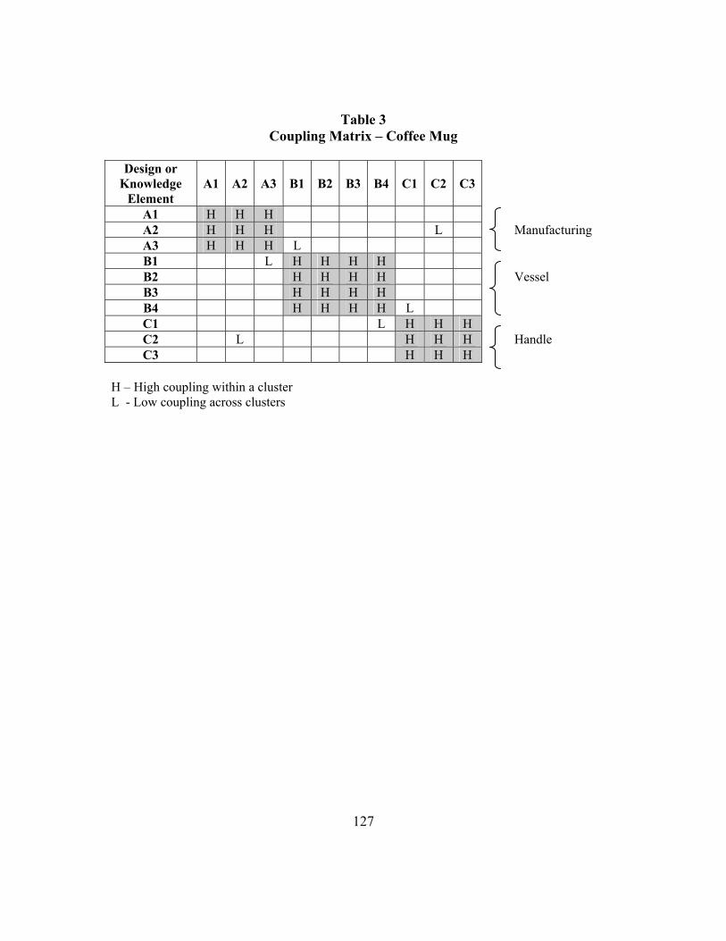
Table 3 Coupling Matrix – Coffee Mug

Design or

Knowledge Element

A1 A2 A3 B1 B2 B3 B4 C1 C2 C3

A1 H H H A2 H H H L Manufacturing A3 H H H L B1 L H H H H B2 H H H H Vessel B3 H H H H B4 H H H H L C1 L H H H C2 L H H H Handle C3 H H H

H – High coupling within a cluster L - Low coupling across clusters

127

Table 4 Interdependence vs. coupling

Interdependence Coupling

Inherent relationship between elements

Not known a priori

May not be low

Decision taken on how the search across two interdependent elements should be combined

Exists in the natural world or the world of natural laws

Exists in the made world or the world of artifacts

Uncovering interdependencies and making valuable guesses on interdependencies is a key aspect of technological search

Mechanism for uncovering interdependencies

e.g., handle shape of the coffee mug is dependent on the width of the walls, height and diameter of the vessel

e.g., how closely tied is the design of the handle of the coffee mug to the design of the vessel

128

Table 5

Example of a N=3, K=2 landscape

Configuration of the System

Value

State of Node 1

State of Node 2

State of Node 3

Value of Node

1

Value of Node

2

Value of Node

3

Total Value of the System

s1 s2 s3 c1 c2 c3 C=Σ ci / N

0 0 0 .6 .3 .5 .47

0 0 1 .1 .5 .9 .50

0 1 0 .4 .8 .1 .43

0 1 1 .3 .5 .8 .53

1 0 0 .9 .9 .7 .83*

1 0 1 .7 .2 .3 .40

1 1 0 .6 .7 .6 .63

1 1 1 .7 .9 .5 .70*

* - Local peak

Arrows point in the direction of increasing values.

000(0.47)

101(0.40)

100(0.83)

110(0.63)

010(0.43) 011

(0.53)

001(0.50)

111(0.70)

000(0.47)

101(0.40)

100(0.83)

110(0.63)

010(0.43) 011

(0.53)

001(0.50)

111(0.70)

129

Table 6 Comparison of studies that have used the NK model

System Studies Nodes Issues addressed

Organization Levinthal (1997)

Sub-units within an organization

How does the coupling between the sub-units affect the survival of the organization?

Technology landscape

Kauffman et al (2000); Fleming and Sorenson, (2001a)

Technology recipes or components

Search on the technology landscape: local search vs. distant search; the effect of N and K on usefulness of inventions

Strategy Rivkin (2000; 2001)

Components of a strategy Effect of the number of interactions between the components (~ complexity of the strategy) on the imitatability and replicability of the strategy, when components can be copied, but less than perfectly.

Economy Kauffman et al (1994), Levitan et al (1999)

Decisions or tasks or activities; A cluster of nodes represents a hierarchy

How should the decisions be coordinated? What is the optimal organization size?

130

Table 7 Summary of Hypotheses

Level of analysis: Firm

Hypothesis Independent variable Dependent variable Relationship Hypothesis 1 Integration between clusters,

Integration i,t-3 to t-1 Percentage of exploratory inventions at time t, Percent_Exploratoryi,t

Inverted U

Hypothesis 2 Integration between clusters, Integrationi,t-3 to t-1

Usefulness of inventions at time t, Usefulnessi,t

Inverted U

Hypothesis 4a Integration between clusters, Integrationi,t-3 to t-1

Change in structure, Changet-3 to t-1, t

Inverted U

Hypothesis 4b Use of scientific knowledge, Sci_Usagei, t-3 to t-1

Change in structure, Changet-3 to t-1, t

Linear

Hypothesis 4c Integration between clusters × Use of scientific knowledge, Integration i,t-3 to t-1 × Sci_Usagei, t-3 to t-1

Change in structure, Changet-3 to t-1, t

Inverted U

Level of analysis: Technology class pairs

Hypothesis Independent variable Dependent variable Relationship Hypothesis 3a Success of exploratory patents

that combine classes j and k, Success_Exploratoryi, j-k, t-3 to t-1

Increase/ Decrease in the coupling between classes j and k, Increase_Li, j-k, t , Decrease_Li, j-k, t

Linear

Hypothesis 3b Percentage of exploratory patents that combine classes j and k, Perc_Sciencei, j-k, t-3 to t-1

Increase/ Decrease in the coupling between classes j and k, Increase_Li, j-k, t , Decrease_Li, j-k, t

Linear

131

TABLE 8

132

le 7 8 9 10 11 12Descriptive Statistics and Correlations for Firm Level of Analysis a,b

ean . in ax. 1 2 3 4 5 6Variab M s d. M . M

1. Number of citations 684.19 1242.33 0 7633

2. Number of patents 85.71 155.88 0 1042 0.88*

3. Number of patents in patent portfolio 202.16 369.01 1 2206 0.85* 0.97*

4.

Integration betweenclusters 0.16 0.16 0 1 -0.30* -0.31* -0.31*

5. Reliance on science 0.41 0.24 0 1 0.08* 0.07 0.08* -0.06

6. Technology control 671.92 1189.04 0 6569 0.97* 0.93* 0.90* -0.31* 0.07

7. Research intensity 0.14 0.47 0 7.97 -0.06 -0.06 -0.06 0.05 0.05 -0.06

8. Firm size 43716.82 90016.44 22 593000 0.58* 0.51* 0.56* -0.26* 0.13* 0.58* -0.07

9. Firm performance -0.07 0.94 -15.5 0.33 0.06 0.06 0.05 -0.02 -0.01 0.06 -0.97* 0.05

10. Product diversification -15.52 0.50 0 1 0.24* 0.33* 0.34* -0.17* -0.12* 0.33* -0.15* 0.27* 0.09*

11. Non-American firm 0.27 0.44 0 1 0.21* 0.33* 0.34* -0.08 -0.13* 0.33* -0.10* 0.16* 0.06 0.67*

12. Level of exploration 0.16 0.17 0 1 -0.14* -0.14* -0.14* 0.12* 0.02 -0.13* -0.03 -0.04 0.03 -1e-3 -0.01

13. Change in structure 24.43 21.48 0 179.2 0.27* 0.28* 0.27* -0.30* 0.12* 0.24* -0.07 0.22* 0.09* 0.06 -0.05 -0.08a n=639 firm years b All independent variables except for number of patents are lagged by one year * p<.05

TABLE 9 Results of Fixed Effects Analyses for Level of Exploration

Variable Model 1 Model 2 Model 3 Model 4 Model 5

Constant -2.52 *** -2.69 *** -3.02 *** -4.37 *** -2.05*** 0.45

0.46 0.46 0.60 0.38

Integration between clusters

0.94 † 6.28 *** 7.21 *** 4.01** 0.55 1.54 2.01 1.27

Integration between clusters squared -10.77 *** -9.89 * -7.05** 2.91 3.80 2.41

Number of patents

-2.70E-03 ** -2.67E-03 ** -2.33E-03 ** -2.64E-03 * -1.40E-03*8.02E-04 8.00E-04 7.94E-04 1.04E-03 6.57E-04

Research Intensity

-1.50E-03 -0.02 0.07 0.49 -2.02* 1.05 1.05 1.04 1.35 0.86

Firm size

1.16E-06 1.14E-06 1.14E-06 -1.28E-07 1.19E-062.87E-06 2.86E-06 2.82E-06 3.68E-06 2.33E-06

Firm performance

-3.85E-03 -0.03 0.06 0.20 -0.95* 0.47 0.47 0.47 0.61 0.39

Product diversification

-0.31 -0.35 -0.43 -0.53 -0.430.36 0.36 0.36 0.47 0.30

1985 -0.11 -0.10 -0.08 0.03 -0.070.31 0.31 0.30 0.39 0.25

1986 -0.17 -0.16 -0.10 -0.11 -0.120.30 0.30 0.30 0.39 0.25

133

134

1987 -0.47 -0.45 -0.34 -0.28 -0.220.30 0.30 0.30 0.39 0.25

1988 -0.01 0.02 0.04 0.01 0.080.30 0.30 0.30 0.39 0.25

1989 -0.05 -0.03 -0.03 -0.31 0.060.30 0.30 0.30 0.39 0.25

1990 -0.10 -0.08 -0.07 -0.09 -4.90E-030.31 0.31 0.30 0.39 0.25

1991 -0.27 -0.23 -0.20 -0.34 -0.100.31 0.31 0.30 0.39 0.25

1992 0.14 0.17 0.24 0.24 0.280.31 0.31 0.30 0.39 0.25

1993 0.36 0.37 0.40 0.18 0.400.31 0.31 0.30 0.40 0.25

1994 0.26 0.29 0.33 0.31 0.49†0.32 0.32 0.32 0.41 0.26

Number of observations 568 568 568 568 568

Number of groups 85 85 85 85 85a All regressions include class dummies for which results have not been displayed. † p <.10 * p <.05 ** p <.01 *** p <.001

TABLE 9 (CONTINUED) Results of Fixed Effects Analyses for Level of Exploration

Variable Model 6 Model 7 Model 8

Constant -4.17 *** ***-5.91 -2.54 *** 0.34 0.90 0.42

Integration between clusters 5.37 *** 7.82 *** 3.66 *** 1.02 2.05 1.01

Integration between clusters squared -7.92 *** -8.57 ** -4.18 ** 1.60 3.17 1.34

Number of patents -2.61E-03 ** -0.01 ** -1.56E-03 * 7.93E-04 2.57E-03 6.51E-04

Research Intensity 1.77 -1.39 1.96 0.86

Firm size -1.10E-05 * 8.22E-07 5.23E-06 2.32E-06

Firm performance 0.84 -0.68 † 0.88 0.39

Product diversification 0.01 -1.95 ** -0.38 0.26 0.71 0.29

1985

0.11 -0.69 -0.02 0.28 0.60 0.25

1986 0.13 -0.57 -0.14 0.27 0.60 0.25

1987 -0.12 -0.60 -0.20

135

136

0.27 0.60 0.25

1988 0.32 -0.90 -0.01 0.26 0.60 0.25

1989 0.34 -0.84 -0.03 0.26 0.60 0.25

1990 0.18 **-1.61 -0.05 0.27 0.60 0.25

1991 -0.02 †-1.16 -0.11 0.27 0.60 0.25

1992 0.44 -0.94 0.19 0.27 0.60 0.25

1993 0.48 † -0.75 0.26 0.27 0.60 0.25

1994 0.53 † -0.72 0.27 0.29 0.64 0.26

Number of observations 759 501 568

Number of groups 115 75 85 a All regressions include class dummies for which results have not been displayed. † p <.10 * p <.05 ** p <.01 *** p <.001

TABLE 10 Results of Fixed Effects Negative Binomial Regression Analyses for Number of Citations

Model 1 Model 2 Model 3 Model 4 Model 5 Model 6 Model 7

Constant -0.04 0.24 0.07 0.21

Variable

0.07 0.15 0.050.15

0.15 0.16 0.16 0.16 0.14 0.17

Integration between clusters

-1.11*** 1.66* * 1.10 1.60** 1.74*0.26 0.75 0.76 0.75 0.58 0.76

Integration between clusters squared

-5.72*** -5.83*** -5.00** -3.96*** -5.73***1.54 1.56 1.51 1.05 1.54

Number of patents

6.74E-04* 6.44E-04* 7.12E-04* 7.30E-04* 1.05E-03***

4.02E-04 6.87E-04*2.92E-04 2.84E-04 2.82E-04 2.83E-04 2.49E-04 3.11E-04 2.77E-04

Research Intensity

1.61** 1.58** 1.56** 1.59** 1.14** 1.68**0.50 0.48 0.47 0.47 0.43 0.49

Firm size

3.29E-06***

3.07E-06***

3.06E-06***

3.04E-06***

2.87E-06***

3.02E-06*** 4.34E-07 4.29E-07 4.34E-07 4.34E-07 4.47E-07 5.05E-07

Firm performance

0.70** 0.69** 0.69** 0.71** 0.50* 0.75**0.23 0.22 0.22 0.22 0.20 0.23

Product diversification

0.41** 0.39** 0.33** 0.32** 0.39** 0.54*** 0.67***0.12 0.12 0.12 0.12 0.11 0.09 0.12

Non-American

0.37* 0.33† 0.35† 0.30† 0.31† -0.43*** 0.000.18 0.18 0.18 0.18 0.18 0.10 0.19

Technology control

3.30E-04***

3.26E-04***

3.30E-04***

3.32E-04***

2.95E-04***

4.53E-04***

3.16E-04*** 4.52E-05 4.40E-05 4.39E-05 4.41E-05 3.97E-05 4.58E-05 4.43E-05

1985

0.13 0.12 0.12 0.13 0.16 -0.08 0.140.12 0.12 0.12 0.12 0.13 0.13 0.12

1.76

137

138

1986

0.25* 0.25* 0.25* 0.26* 0.27* 0.12 0.23*0.12 0.11 0.11 0.11 0.13 0.12 0.11

1987

0.27* 0.25* 0.25* 0.25* 0.32* 0.16 0.25*0.12 0.11 0.11 0.11 0.13 0.12 0.11

1988

0.21† 0.18 0.18 0.18 0.32* 0.10 0.20†0.12 0.12 0.12 0.12 0.13 0.12 0.12

1989

0.18 0.16 0.16 0.16 0.42** 0.01 0.21†0.12 0.12 0.12 0.11 0.12 0.12 0.12

1990

0.07 0.04 0.04 0.05 0.44*** -0.16 0.100.12 0.12 0.12 0.12 0.12 0.12 0.12

1991

0.07 0.02 0.03 0.03 0.54*** -0.12 0.090.12 0.12 0.12 0.12 0.12 0.12 0.12

1992

0.01 -0.04 -0.03 -0.04 0.57*** -0.16 0.040.12 0.12 0.12 0.12 0.12 0.12 0.12

1993

1.8e-03 -0.03 -4.5E-03 -0.02 0.61*** -0.09 0.060.13 0.12 0.12 0.12 0.13 0.12 0.12

1994

-0.07 -0.11 -0.09 -0.10 0.48*** -0.20 -0.030.14 0.13 0.13 0.13 0.14 0.13 0.13

Log Likelihood -2932.91 -2923.49 -2914.4 -2854.33 -2714.93 -3873.87 -2835.58

Number of observations 617 617 617 617 617 847 604

Number of groups 85 85 85 85 85 115 81† p <.10 * p <.05 ** p <.01 *** p <.001

TABLE 10 (CONTINUED) Results of Fixed Effects Negative Binomial Regression Analyses for Number of Citations

Variable Model 8 Model 9 Model 10 Model 11 Model 12 Model 13

Constant -0.17 ***-0.95 -0.33* ***-0.77 -0.57** -0.38* 0.15

0.15 0.15 0.17 0.18 0.19

Integration between clusters

1.15† 6.00*** 1.62** 2.34** 2.82*** 4.96***0.68 0.90 0.51 0.81 0.65 0.78

Integration between clusters squared

-3.67** -11.64*** -3.58*** -5.28** -5.03*** -7.07***1.35 2.02 0.57 1.58 1.07 1.07

Number of patents

1.74E-03***

6.08E-04† 6.93E-04* 3.96E-04 2.22E-03***

8.80E-04** 1.15E-04 3.25E-04 3.01E-04 3.29E-04 5.38E-04 2.76E-04

Research Intensity

1.43** 1.87*** 2.10*** 2.03*** 1.83** 1.89***0.42 0.43 0.47 0.42 0.57 0.47

Firm size

4.59E-07 3.84E-06***

3.48E-06***

3.80E-06***

3.63E-06***

2.92E-06*** 3.72E-07 4.61E-07 4.44E-07 4.53E-07 4.92E-07 4.29E-07

Firm performance

0.60** 0.83*** 0.93*** 0.89*** 0.88** 0.83***0.20 0.20 0.22 0.20 0.28 0.22

Product diversification

-0.04 0.47*** 0.47*** 0.56*** 0.34* 0.27* 0.08 0.13 0.12 0.13 0.14 0.11

Non-American

0.26 0.43* **0.50 *0.43 **0.72 †0.320.18 0.18 0.18 0.18 0.21 0.18

Technology control

Class 3.78E-04***

3.48E-04***

3.84E-04***

4.62E-04***

2.99E-04*** dummies 4.94E-05 4.62E-05 4.93E-05 7.83E-05 4.32E-05

1985

0.01 0.07 0.10 0.04 0.12 0.170.07 0.14 0.13 0.14 0.14 0.12

139

140

1986

0.05 0.26* 0.24* 0.23† 0.31* 0.24*0.07 0.13 0.12 0.13 0.13 0.11

1987

0.08 0.26* 0.23† 0.24† 0.35** 0.27*0.07 0.13 0.12 0.13 0.13 0.11

1988

0.04 0.24† 0.18 0.22† 0.23† 0.20†0.07 0.13 0.12 0.13 0.13 0.11

1989

-0.01 0.17 0.11 0.16 0.20 0.150.07 0.13 0.12 0.13 0.13 0.11

1990

-0.10 0.12 0.04 0.10 0.07 0.060.07 0.13 0.12 0.13 0.13 0.11

1991

-0.17* 0.13 0.03 0.11 0.04 0.020.07 0.13 0.12 0.13 0.14 0.11

1992

-0.40*** 0.12 -4.9E-04 0.11 0.00 -0.050.07 0.13 0.13 0.13 0.13 0.12

1993

-0.55*** 0.13 -4.7E-03 0.11 -0.04 -0.040.08 0.14 0.13 0.14 0.14 0.12

1994

-0.89*** 0.08 -0.08 0.07 -0.20 -0.170.08 0.15 0.14 0.15 0.15 0.13

Log Likelihood -2705.5 -3134.99 -3101.99 -3156.67 -2463.53 -2906.73

Number of observations 617 739 739 739 561 617

Number of groups 85 89 89 89 74 85† p <.10 * p <.05 ** p <.01 *** p <.001

TABLE 11 Descriptive Statistics and Correlations for Technology class pair Level of Analysis a

141

Variable Mean s.d. Min. Max. 1 2 3 4 5 6 7 8 9

1 Increase in coupling 0.05 0.21 0 1

2 Decrease in coupling 0.03 0.16 0 1 -0.04*

3 Average citation rate 5.91 7.13 0 136 0.03* -0.05*

4 Average use of scientific knowledge 0.46 0.48 0 1 -0.01 -0.04* 0.10*

5 Number of patents that cite class pair in previous time period 1.20 0.59 1 11 0.02* -0.03* 0.00 0.01

6 Research Intensity 0.10 0.15 0 5.36 0.01* -0.02* 0.06* 0.01 0.01

7 Firm size 119889.10 141219.60 18.67 756193 -0.05* -0.04* -0.04* 0.07* -0.03* -0.13*

8 Firm performance 0.02 0.29 -10.29 0.22 4.50E-03 2.70E-03 0.01 2.60E-03 1.00E-04 -0.95* 0.07*

9 Product diversification 0.69 0.46 0 1 -0.05* 0.04* -0.19* -0.10* 4.90E-03 -0.18* -0.08* 0.06*

10 Non-American 0.46 0.50 0 1 -0.04* 0.03* -0.15* -0.08* 0.03* -0.05* -0.02* 0.02* 0.61*a n=26589 technology class pair years * p<.05

TABLE 12 Results of Random Effects Regression Analyses for Change in Coupling between Technology Class Pairsa

Variable

Model 1 Increase in

coupling

Model 2 Decrease in

coupling

Model 3 Increase in

coupling

Model 4 Decrease in

coupling

Model 5 Increase in

coupling

Model 6 Increase in

coupling

Model 7 Decrease in

coupling

Constant -5.09*** -7.32*** -5.05*** -11.22*** -4.63*** -5.24*** 1.97*** 0.33

0.72 0.24 0.60 0.17 0.15 0.10

Average of citations received

0.02** -0.11*** 0.03*** -0.16*** 0.02*** 0.02*** -0.04***0.01 0.02 0.01 0.02 3.04E-03 2.65 E-03 2.54 E-03

Average use of scientific knowledge

-0.16 -0.73** -0.14 -0.53* -0.02 -4.95E-03

-0.09* 0.10 0.26 0.09 0.22 0.05 0.04 0.03

Coupling between class pair in previous time period

-0.11 0.24 -0.02 0.40** -0.22*** -0.64*** 0.03***0.07 0.15 0.07 0.15 0.03 0.02 0.00

Across cluster tie

0.31***

-5.96*** 0.05 0.09

Research Intensity

2.98** -25.47*** 3.11*** 4.83*** -8.93***1.05 4.13 0.63 0.54 0.53

Firm size

-2.48E-06***

-8.49E-06***

-5.66E-07** 4.31E-07* -3.61E-06*** 4.23E-07 1.41E-06 2.01E-07 1.74E-07 1.66E-07

Firm performance

1.56** -7.06*** 1.67*** 2.53*** -4.34***0.52 1.27 0.33 0.29 0.27

Product diversification

-0.41** -0.77† -0.68*** 0.19 -0.27*** -0.19** -0.050.15 0.42 0.10 0.25 0.08 0.07 0.06

Non-American

-0.15 1.02** 0.08 0.78** -0.08 -0.02 -0.51***0.14 0.38 0.10 0.24 0.07 0.06 0.06

142

143

1985

0.25 -0.29 0.26 -0.33 0.16 0.10 -0.050.23 0.44 0.19 0.39 0.12 0.11 0.07

1986

0.35 -0.12 0.36† -0.23 0.35** 0.26* -0.31***0.23 0.45 0.19 0.40 0.12 0.11 0.07

1987

0.10 -0.31 0.13 -0.56 0.28* 0.23* -0.44***0.24 0.45 0.20 0.41 0.12 0.11 0.07

1988

0.25 -0.24 0.44* -0.45 ***0.46 0.37** -0.59***0.23 0.46 0.19 0.40 0.12 0.11 0.07

1989

-0.43† -1.21* -0.30 -1.38** 0.28* 0.26* -0.56***0.24 0.48 0.20 0.42 0.12 0.11 0.06

1990

-0.19 -1.36** -0.04 -1.37** 0.24* 0.23* -0.53***0.23 0.47 0.19 0.42 0.12 0.11 0.06

1991

-0.24 -1.42** -0.08 -1.45** 0.39** 0.35** -0.57***0.23 0.48 0.19 0.42 0.12 0.11 0.06

1992

0.27 ***-1.67 0.41* -1.72*** 0.93*** 0.84*** -0.88***0.22 0.47 0.18 0.41 0.12 0.11 0.06

1993

0.62** -1.81*** 0.66*** -1.74*** 1.27*** 1.18*** -1.11***0.22 0.47 0.18 0.41 0.12 0.10 0.06

Number of observations 26589 26589 29789 29789 67796 135500 135500

Number of groups 12648 12648 14076 14076 22173 36734 36734

Log Likelihood -4590.21 -2213.76 -5426.38 -2560.46 -15759.64 -18770.52 -55376.76a All regressions include dummies for each firm class pair for which results have not been displayed. † p <.10 * p <.05 ** p <.01 *** p <.001

TABLE 13

Results of Fixed Effects Regression Analyses for Change in Structurea

Model 1 Model 2 Model 3 Model 4 Model 5 Model 6

Constant 2.45 *** 2.49 *** 2.34 ****** 2.16 2.16 *** 2.14 *** 0.32

1.44 3.44

0.32 0.32 0.32 0.32 0.32Integration between clusters

-0.22 1.41 ** 1.19 * 1.17 * 1.21 * 0.21 0.52 0.52 0.55 0.56

Integration between clusters squared

-2.84 ** -2.46 ** -2.44 ** -2.54 ** 0.84 0.84 0.88 0.92

Use of scientific knowledge

0.50 ** 0.50 ** 0.54 ** 0.17 0.17 0.19

Integration between clusters × Use of scientific knowledge

0.08 0.35 0.73 0.98

Integration between clusters squared × Use of scientific knowledge

-

Number of patents in patent portfolio

-1.27E-04 -1.33E-04 -7.41E-05 -1.05E-04 -1.05E-04 -1.01E-04 1.63E-04 1.63E-04 1.62E-04 1.60E-04 1.61E-04 1.61E-04

Research Intensity

-2.61 ** -2.63 ** -2.56 ** -2.78 ** -2.77 ** -2.77 **0.97 0.97 0.96 0.95 0.95 0.96

Firm size

1.45E-08 1.33E-08 -1.57E-08 -9.63E-09 -7.57E-09 -1.33E-088.40E-07 8.40E-07 8.29E-07 8.21E-07 8.22E-07 8.23E-07

Firm performance

-1.15 ** -1.16 ** -1.14 ** -1.25 ** -1.25 ** -1.25 **0.43 0.43 0.42 0.42 0.42 0.42

Product diversification

0.08 0.08 0.06 0.11 0.11 0.110.17 0.17 0.17 0.16 0.17

144

0.17

145

Non-American

0.31 0.33 0.44 0.41 0.41 0.420.79 0.79 0.78 0.77 0.77 0.78

1985 0.16 0.16 0.15 0.15 0.15 0.150.12 0.12 0.11 0.11 0.11 0.11

1986 0.23 * 0.23 * 0.25 * 0.25 * 0.25 * 0.24 *0.11 0.11 0.11 0.11 0.11 0.11

1987 0.22 † 0.21 † 0.23 * 0.22 † 0.22 † 0.22 †0.12 0.12 0.11 0.11 0.11 0.11

1988 0.32 ** 0.31 ** 0.31 ** 0.31 ** 0.31 ** 0.31 **0.12 0.12 0.11 0.11 0.11 0.11

1989 0.28 * 0.27 * 0.26 * 0.25 * 0.25 * 0.25 *0.12 0.12 0.11 0.11 0.11 0.11

1990 0.40 ** 0.39 ** 0.38 ** 0.37 ** 0.37 ** 0.36 **0.12 0.12 0.12 0.12 0.12 0.12

1991 0.41 ** 0.40 ** 0.39 ** 0.38 ** 0.38 ** 0.38 **0.12 0.12 0.12 0.12 0.12 0.12

1992 0.55 *** 0.54 *** 0.54 *** 0.53 *** 0.53 *** 0.53 ***0.12 0.12 0.12 0.12 0.12 0.12

1993 0.60 *** 0.59 *** 0.59 *** 0.61 *** 0.61 *** 0.60 ***0.12 0.12 0.12 0.12 0.12 0.12

Number of observations 527 527 527 527 527 527

Number of groups 85 85 85 85 85 85a All regressions include class dummies for which results have not been displayed. † p <.10 * p <.05 ** p <.01 *** p <.001

TABLE 13 (CONTINUED) Results of Fixed Effects Regression Analyses for Change in Structurea

Model 7 Model 8 Model 9

Constant 2.06 *** 2.03 *** 1.06 † 0.14

0.39 0.61Integration between clusters

1.04 * 1.77 ** 2.14 ***0.44 0.53 0.50

Integration between clusters squared

-2.51 *** -2.72 *** -3.11 ***0.68 0.74 0.66

Use of scientific knowledge

0.39 * 0.57 ** 1.02 ***0.16 0.20 0.24

Integration between clusters × Use of scientific knowledge

-0.69 -0.76 0.260.73 1.00 0.50

Integration between clusters squared × Use of scientific knowledge

1.72 -0.08 -6.19 **2.01 2.11 2.18

Number of patents in patent portfolio

-3.15E-04 * -3.05E-05 -1.21E-04 1.56E-04 3.37E-04 1.52E-04

Research Intensity

-2.06 † -2.21 * 1.20 0.94

Firm size 5.16E-07 0.09 9.80E-07 0.06

Firm performance

-0.93 † -0.96 * 0.53 0.42

Product diversification

-0.01 0.05 0.160.12 0.20 0.16

146

147

Non-American

-0.07 -0.06 0.320.12 0.95 0.75

1985 3.93E-03 0.16 0.20 †0.11 0.14 0.11

1986 0.16 0.19 0.20 †0.10 0.14 0.11

1987 0.17 0.20 0.21 †0.10 0.14 0.11

1988 0.21 * 0.20 0.30 **0.10 0.14 0.11

1989 0.17 † 0.21 0.22 *0.10 0.14 0.11

1990 0.27 ** 0.29 * 0.33 **0.10 0.14 0.11

1991 0.35 ** 0.36 * 0.34 **0.10 0.14 0.11

1992 0.48 *** 0.48 ** 0.47 ***0.11 0.15 0.11

1993 0.64 *** 0.69 *** 0.54 ***0.11 0.15 0.12

Number of observations 719 482 527

Number of groups 115 75 85a All regressions include class dummies for which results have not been displayed. † p <.10 * p <.05 ** p <.01 *** p <.001

Table 14 Proposed effects and findings

Hypothesis Independent

variable Dependent variable Relationship Findings

H1 Integration between clusters

Percentage of exploratory inventions at time t

Inverted U Inverted U

H2 Integration between clusters

Usefulness of inventions at time t

Inverted U Inverted U

H3a Success of exploratory patents that combine classes j and k

Increase/ Decrease in the coupling between classes j and k

Linear Linear

H3b Percentage of exploratory patents that combine classes j and k and cite a non-patent reference

Increase/ Decrease in the coupling between classes j and k

Linear Not significant

H4a Integration between clusters

Change in structure Inverted U Inverted U

H4b Use of scientific knowledge

Change in structure Linear Linear

H4c Integration between clusters × Use of scientific knowledge

Change in structure Inverted U Not significant

148

Figure 1 Determinants of Effectiveness of Technological Search

Knowledge Base • Elements • Structure

Inventions • Usefulness

Where? Domain of search

How? Type of search

149

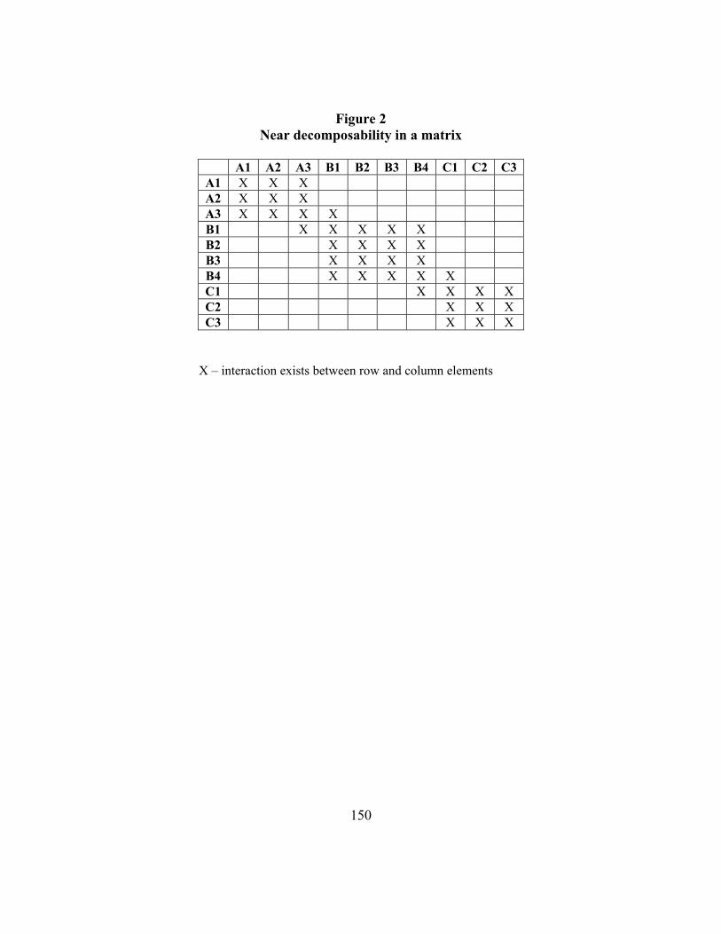
Figure 2 Near decomposability in a matrix

A1 A2 A3 B1 B2 B3 B4 C1 C2 C3

A1 X X X A2 X X X A3 X X X X B1 X X X X X B2 X X X X B3 X X X X B4 X X X X X C1 X X X X C2 X X X C3 X X X

X – interaction exists between row and column elements

150

Figure 3 Interdependence and coupling

a) Interaction matrix for two-way interdependencies (K=2)

A1 A2 A3 B1 B2 B3 B4 C1 C2 C3

A1 X X X X X X A2 X X X X A3 X X X X X B1 X X X X X X X B2 X X X X X B3 X X X X B4 X X X X X X C1 X X X X C2 X X X X X C3 X X X X

X – Row and column elements are interdependent

b) Coupling matrix with near decomposability

A1 A2 A3 B1 B2 B3 B4 C1 C2 C3

A1 H H H A2 H H H L A3 H H H L B1 L H H H H B2 H H H H B3 H H H H B4 H H H H L C1 L H H H C2 L H H H C3 H H H

H – High Coupling L- Low Coupling

151

152

Figure 4

Broad alternatives for coupling (adapted from Kauffman (1995:255))

A

B

C

D

A nearly

decomposable system

High

within cluster and

low between clusters

4

4

A system that combines

decentralization at a global level

with centralization at the local level

Perfect within

cluster and zero

between all nodes

4

4

A perfectly centralized

system

Perfect between all the nodes

1

16

A perfectly decentralized

system

Zero between all the nodes

16

1

Interpretation Coupling(L)

Number of clusters (J)

Cluster size (NJ)

153

Figure 5 Mean payoffs for various levels of coupling

(J = Number of clusters)

(Continued…)

N=12, K=6

0.64

0.66

0.68

0.7

0 0.2 0.4 0.6 0.8 1

Coupling between clusters

Mea

n Pa

yoff

J=2J=3J=6J=12

N=12, K=4

0.64

0.66

0.68

0.7

0 0.2 0.4 0.6 0.8 1

Coupling between clusters

Mea

n Pa

yoff

J=2J=3J=6J=12

154

Figure 5 (Contd.) Mean payoffs for various levels of coupling

(J = Number of clusters)

N=12, K=8

0.64

0.66

0.68

0.7

0 0.2 0.4 0.6 0.8 1

Coupling between clusters

Mea

n Pa

yoff

J=2J=3J=6J=12

N=12, K=11

0.64

0.66

0.68

0.7

0 0.2 0.4 0.6 0.8 1

Coupling between clusters

Mea

n Pa

yoff

J=2J=3J=6J=12

155

Figure 6 Standard deviations of mean payoffs

(J = Number of clusters)

N=12, K=11

0.04

0.06

0.08

0.1

0 0.2 0.4 0.6 0.8 1

Coupling between clusters

S.D

. (Pa

yoff

)

J=2J=3J=6J=12

N=12, K=4

0.04

0.06

0.08

0.1

0 0.2 0.4 0.6 0.8 1

Coupling between clusters

S.D

. (Pa

yoff

)

J=2J=3J=6J=12

156

Figure 7 Payoff of local optimum vs. number of times each local optimum was attained

N=12, K=11

Coupling between groups = .08

0.4

0.5

0.6

0.7

0.8

0 100 200 300

Number of times optimum is attained

Mea

n pa

yoff

Coupling between groups = .1

0.4

0.5

0.6

0.7

0.8

0 50 100 150 200

Number of times optimum is attained

Mea

n pa

yoff

Coupling between groups = .2

0.4

0.5

0.6

0.7

0.8

0 50 100

Number of times optimum is attainedM

ean

payo

ff

Coupling between groups = 1

0.4

0.5

0.6

0.7

0.8

0 10 20 30

Number of times optimum is attained

Mea

n pa

yoff

157

Figure 8 Mean walk length to local optima and percentage of walks that reached local

optima

a) N=12, K=11

1

10

100

1000

0 0.2 0.4 0.6 0.8 1

Coupling between clusters

Mea

n w

alk

leng

th to

opt

ima J=2

J=3J=6J=12

N=

20

40

60

80

100

0 0.05

Coupling be

Perc

enta

ge o

f wal

ks th

at

reac

hed

a lo

cal o

ptim

um

1

)

b

0

tw

2, K=11

.1 0.15 0.2

een clusters

J=2J=3J=6J=12

158

Figure 9 Distribution of walk lengths

N=12, K=11

0

0.5

1

1.5

2

2.5

3

0 1 2 3

Log (Walk Length)

Log

(Fre

quen

cy)

Coupling between clusters = 1

0

0.5

1

1.5

2

2.5

3

0 1 2 3

Log (Walk Length)

Log

(Fre

quen

cy)

Coupling between clusters = .08

0

0.5

1

1.5

2

2.5

3

0 1 2 3

Log (Walk Length)

Log

(Fre

quen

cy)

Coupling between clusters = .04

a) b)

c)

159

Figure 10 Mean value vs. length of adaptive walk

N=12, K=11

Coupling between clusters = .04

0.6

0.65

0.7

0.75

1 401 801 1201

Length of adaptive walk

Mea

n pa

yoff

Coupling between clusters = 1

0.6

0.65

0.7

0.75

1 4 7 10

Length of adaptive walk

Mea

n pa

yoff

Coupling between clusters = .08

0.6

0.65

0.7

0.75

1 301 601 901

Length of adaptive walk

Mea

n pa

yoff

160

Figure 11 Model of hypothesized relationships

The Structure of a knowledge base

(Continued…)

Integration between clusters

Usefulness of inventions

H1Percentage of

exploratory inventions

+/-

H2

+/-

161

Figure 11 (Continued)

Changes in the structure of a knowledge base

At the level of the technology-class pairs

At the level of the firm

Intermediate level

of coupling

Use of scientific

knowledge

Integration between clusters

Cognitive Search

H4b

+/-

Changes in the structure of a

knowledge base

H4a

H4c

+/- X

Success of exploratory inventions

H3a

Experiential Search

Change in coupling between

elements

Cognitive Search

Exploratory inventions that use

science H3b

162

Figure 12 Variable Definitions and Operationalizations

Coupling matrix, Li, t-3 to t-1 C1 C2 C3 C4 C1 C2 C3 C4 C1 1 C1 1 C2 2/(2+0+1) 1 = C2 2/3 1 C3 0/(0+2+3) 1/(1+2+2) 1 C3 1/5 1 C4 0/(0+2+2) 0/(0+2+3) 2/(2+0+1) 1 C4 2/3 1

Each cell is the similarity between the row technology class and the column technology class measured as the Jaccard’s coefficient (Everitt, 1993). Jaccard’s Coefficient = a/(a+b+c)

where a = number of patents in which the two classes are used together b = number of times class 1 is used, but class 2 is not used

c = number of times class 2 is used, but class 1 is not used

(Continued…)

Cited patentsin t-3 to t-1

Technology classes to which

cited patents belong

C1

C2

C1

C2

Patents int-3 to t-1

Patent 10

Patent 11

Patent 8

Patent 9 Patent 1

Patent 3

Patent 1

Patent 2

Patent 3

Patent 4

Patent 4

Patent 5

C2

C3

C3

C4

Patent 6

Patent 7

C3

C4 Patent 12

Patent 15

Patent 13

Patent 14

Patents in t Citing patents, t+1 to 1999

Patent 18

Patent 19

Patent 16

Patent 17

Patent 20

163

Figure 12 (Contd.)

Coupling matrix visualized as a network

Nodes represent technology classes A tie represents coupling between two technology classes Strength of tie is given by level of coupling • Dark lines – Strong ties • Light lines – weak ties Clustering coefficient

Node Number of neighbors

Number of possible ties between neighbors

Number of actual ties between neighbors

Clustering coefficientnode

A 2 1 1 1 B 2 1 1 1 C 4 6 2 0.33 D 3 3 2 0.66 E 2 1 1 1 F 3 3 2 0.66

D

CA

F

B

E

Clustering coefficient = Number of actual ties / Number of possible ties between neighbors = Σ Clustering coefficientnode / number of nodes = (1+1+0.33+0.66+1+0.66)/6 = 0.78

(Continued…)

Figure 12 (Contd.)

Integration between clusters 1. Classify ties as weak and strong ties based on a cutoff value. In the above figure, the ties between node C and node D, between node D and node E and between node C and node F are classified as weak ties while the other ties are classified as strong ties. 2. For each node identify nodes that are outside its cluster.

Method 1: two nodes belong to the same cluster if a. They have a strong tie between them and there is at least one common node to which

both are tied. b. They have a strong tie between them and both nodes do not have any other ties at all c. They have a weak tie and there exists at least one node to which both are strongly tied. Method 2: Two nodes belong to the same cluster if they have a strong tie

3. For each node calculate its integration with nodes outside its cluster as

gggwhnIntegratio node

+−×+

=

2)1(

where number of neighboring nodes which are outside the focal node's cluster number of ties between neighboring nodes that are outside the focal node's cluster

= number of all nodes to which focal node is connected such that

=h=w

g2

)1( −× gg is the

maximum possible number of ties between the nodes to which focal node is connected.

Node or Tech. Class

Neighbors within cluster

Neighbors outside cluster according to Method 1

Number of neighbors outside cluster, h

Number of actual ties between neighbors outside cluster, w

Number of possible ties between neighbors + Number of ties, (g × (g-1))/2 + g

Integrationnode

A B,C - 0 0 1+2=3 (0+0)/3 = 0 B A,C - 0 0 1+2=3 (0+0)/3=0 C A,B D,F 2 1 6+4=10 (2+1)/10=0.3 D E,F C 1 0 3+3=6 (1+0)/6=0.16 E D,F - 0 0 1+2=3 (0+0)/3=0 F D,E C 1 0 3+3=6 (1+0)/6=0.16

4. Integration i, t-3 to t-1 = Σj Integrationnode j × Number of patents that cite node (or class) j That is, integration between clusters for firm i is the weighted sum of the integration for each node with the number of patents that cite each class as the weight.

164

REFERENCES

Ahuja, G. 2000. Collaboration networks, structural holes, and innovation: A longitudinal study. Administrative Science Quarterly. 45: 425-455.

Ahuja, G. and Lampert, C.M. 2001. Entrepreneurship in the large corporation: a longitudinal study of how established firms create breakthrough inventions. Strategic Management Journal. 22: 521-543.

Ahuja and Katila, 2001. Technological acquisitions and the innovation performance of acquiring firms: a longitudinal study, Strategic Management Journal. 22: 197-220.

Ahuja and Katila, 2002. Searching distant domains: How geography and science search promote innovation. Working Paper.

Albert, M., Avery, D., Narin, F., & McAllister, P. 1991. Direct validation of citation counts as indicators of industrially important patents. Research Policy, 20: 251-259

Allen, T.J., 1977. Managing the flow of technology: Technology transfer and the dissemination of technological information within the R&D organization. MIT Press: Cambridge, MA.

Almeida, P. and Kogut, B. 1999. Localization of knowledge and the mobility of engineers in regional networks. Management Science. 45: 905-917.

Argyres, N. 1996. Capabilities, technological diversification and divisionalization. Strategic Management Journal. 17: 395-410.

Auerswald, P., Kauffman, S., Lobo, J. and Shell, K. 2000. The production recipes approach to modeling technological innovation: An application to learning by doing. Journal of Economic Dynamics and Control. 24: 389-450.

Baldwin, C. and Clark, K. 1997. Managing in the age of modularity. Harvard Business Review. September/ October: 84-93.

165

Baldwin, C. and Clark, K. 2000. Design rules: The power of modularity. MIT Press: Cambridge, MA.

Barabasi, A. 2002. Linked: The new science of networks. Perseus Publishing: Cambridge, MA.

Brown, S.L. and Eisenhardt, K.M. 1997. The art of continuous change: Linking complexity theory and time-paced evolution in relentlessly shifting organizations. Administrative Science Quarterly. 42: 1-34.

Brusoni, S., Prencipe, A. and Pavitt, K. 2001. Knowledge specialization, organizational coupling, and the boundaries of the firm: Why do firms know more than they make? Administrative Science Quarterly. 46: 597-621.

Cameron, A. and Trivedi, P. 1986. Econometric models based on count data: Comparisons and applications of some estimators and tests. Journal of Applied Econometrics. 1: 29-53.

Chang, S.J. 1996. An evolutionary perspective on diversification and corporate restructuring: Entry, exit, and economic performance during 1981-89. Strategic Management Journal. 17: 587-611.

Chang, K. 2002. A New System for Storing Data: Think Punch Cards, but Tiny. New York Times. June 11, 2002.

Cohen, M.D. 1981. The power of parallel thinking. Journal of Economic Behavior and Organization. 2: 285-306.

Cohen, W.M. and Levinthal, D.A. 1990. Absorptive capacity: A new perspective on learning and innovation. Administrative Science Quarterly. 35: 128-152.

Dosi, G. 1988. Sources, procedures, and microeconomic effects of innovation. Journal of Economic Literature. 26: 1120-1171.

Ethiraj, S.K. and Levinthal, D. 2003. Modularity and innovation in complex systems. Management Science. 50: 159-173.

Everitt, B.S., Cluster Analysis (3rd ed.). London: Edward Arnold.

Fleming, L. 2001. Recombinant uncertainty in technology search. Management Science. 47: 117-132.

166

Fleming, L. and Sorenson, O. 2001a. Technology as a complex adaptive system: Evidence from patent data. Research Policy. 30: 1019-1039.

Fleming, L. and Sorenson, O. 2001b. Science as a map in technological search. Working Paper.

167

Science. 40: 1720-1747.

Henderson, R.M. and Clark, K.B. 1990. “Architectural innovation: The reconfiguration of existing product technologies and the failure of established firm”. Administrative Science Quarterly. 35: 9-30.

Galunic, D.C. and Eisenhardt, K.M. 2001. Architectural innovation and modular corporate forms. Academy of Management Journal. 44: 1229-1249.

Garud, R. and Kumaraswamy, A. 1995. Technological and organizational designs for realizing economies of substitution. Strategic Management Journal. 16: 93-109.

Gavetti, G., Levinthal, D. 2000. Looking forward and looking backward: Cognitive and experiential search. Administrative science Quarterly, 45: 113-137.

Galbraith, J.R. 1973. Designing complex organizations. Addison-Wesley, Reading, MA.

Gilfillan, S. 1935. Inventing the ship. Follett Publishing Co., Chicago.

Glassman, R.B. 1973. Persistence and loose coupling in living systems. Behavioral Science. 18: 83-98.

Goldenberg, J., Mazursky, D. and Solomon, S. 1999. Toward identifying the inventive templates of new products: A channeled ideation approach. Journal of Marketing Research. 36: 200-210.

Ghemawat, P. and Levinthal, D. 2000. Choice structures, business strategy and performance: A generalized NK-simulation approach. Working Paper.

Hall, B.H., Jaffe, A. and Tratjenberg, M. 2000. Market value and patent citations: A first look. Working Paper No. 7741, NBER Working Paper Series.

Hall, B.H., Jaffe, A. & Trajtenberg, M. 2001. The NBER patent data citation file: Lessons, insights and methodological tools. Working Paper No. 8498, NBER Working Paper Series. Harhoff, D., Narin, F., Scherer, F.M. & Vopel, K. 1999. Citation frequency and the value of patented innovations. The Review of Economics and Statistics, 81: 511-515.

Helfat, C.E. 1994. Evolutionary trajectories in petroleum firm R&D. Management

168

Coevolutionary problem solving. Working Paper No. 94-06-031, The Santa Fe Institute: Santa Fe

Klevorick, A., Levin, R., Nelson, R. and Winter, S. 1995. On the sources and significance of interindustry differences in technological opportunities. Research Policy. 24: 185-205.

Henderson, R. and Cockburn, I. 1994. Measuring competence? Exploring firm effects in pharmaceutical research. Strategic Management Journal. 15 (Special Issue): 63-84.

Henderson, R. and Cockburn, I. 1996. Scale, scope, and spillovers: The determinants of research productivity in drug discovery. Rand Journal of Economics. 27: 32-59.

Hennart, J. 1993. Explaining the swollen middle: Why most transactions are a mix of market and hierarchy. Organization Science. 4: 529-547.

Hoskisson, R. and Hitt, M. 1988. Strategic control systems and relative R&D investment in large multiproduct firms. Strategic Management Journal. 9: 605-621.

Jaffe, A.B. 1989. Characterizing the “technological position” of firms, with application to quantifying technological opportunity and research spillovers. Research Policy. 18: 87-97.

Jaffe, A.B., Tratjenberg, M. and Henderson, R. 1993. Geographic localization of knowledge spillovers as evidenced by patent citations. The Quarterly Journal of Economics. 108: 577-598.

Kamien, M. and Schwartz, N. 1982. Market structure and innovation. Cambridge University Press: New York.

Katila, R. and Ahuja, G. 2002. Something old, something new: A longitudinal study of search behavior and new product introduction. Forthcoming in Academy of Management Journal.

Kauffman, S. 1993. The origins of order: Self-organization and selection in evolution. Oxford University Press.

Kauffman, S. 1995. At Home in the Universe. New York: Oxford University Press.

Kauffman, S., Lobo, J., & Macready, W.G. 2000. Optimal search on a technology landscape, Journal of Economic Behavior & Organization. 43:141-166.

Kauffman, S., Macready, W.G., & Dickinson, E. 1994. Divide to coordinate:

169

Academy of Management Review. 15: 203-223.

Palepu, K. 1985. Diversification strategy, profit performance and the entropy measure. Strategic Management Journal. 6: 239-255.

Kogut, B. and Zander, U. 1992. Knowledge of the firm, combinative capabilities, and the replication of technology. Organization Science. 3: 383-397.

Lawrence, P.R. and Lorsch, J.W. 1967. Organization and environment: Managing differentiation and integration.

Levinthal, D. A. 1997. Adaptation on rugged landscapes. Management Science. 43: 934-950.

Levinthal, D.A. and March, J.G. 1993. The myopia of learning. Strategic Management Journal. 14: 95-112.

Levinthal, D.A. and Warglien, M. 1999. “Landscape design: Designing for local action in complex worlds”. Organization Science. 10: 342-357.

Levitan, B., Lobo, J., Kauffman, S. and Schuler, R. 1999. Optimal organizational size in a stochastic environment with externalities. Working Paper No. 99-04-024, The Santa Fe Institute.

Levitt, B. and March, J.G. 1988. “Organizational learning”. In W.R. Scott (Ed.), Annual Review of Sociology. 14: 319-340.

March, J.G. 1991. “Exploration and exploitation in organizational learning”. Organization Science. 10: 342-357.

Mokyr, J. 2002. Innovation in an historical perspective: Tales of technology and evolution. In Steil, B., Victor, D.G. and Nelson, R.R. (Eds.) Technological innovation and economic performance: 23-46. Princeton University Press: Princeton.

Narin, F., Noma, E. & Perry, R. Patents as indicators of corporate technological strength. Research Policy, 16: 143-155.

Nelson, R. and Winter, S. 1982. An evolutionary theory of economic change. Harvard University Press, Cambridge, MA.

Orton, J.D. & Weick, K. 1990. Loosely coupled systems: A reconceptualization.

170

Philosophical Society, 106: 467-482.

Simon, H.A. 1996. The sciences of the artificial (3rd Edition). The MIT Press: Cambridge, MA.

Patel, P. and Pavitt, K. 1997. The technological competencies of the world's largest firms: Complex and path-dependent, but not much variety. Research Policy. 26: 141-156. Rivkin, J.W. 2000. Imitation of complex strategies. Management Science. 46: 824-844.

Rivkin, J.W. 2001. Reproducing knowledge: Replication without imitation at moderate complexity. Organization Science. 12: 274-293.

Rivkin, J.W. & Siggelkow, N. 2003. Balancing search and stability: Interdependencies among elements of organizational design. Management Science. 49: 290-311.

Rosenberg, N. 1982. Inside the black box: Technology and economics. Cambridge University Press. Cambridge.

Rosenberg, N. 1992. Science and technology in the twentieth century. In Dosi, G., Giannetti, R. and Toninelli, P. (Eds.). Technology and enterprise in a historical perspective: 63-96. New York: Oxford University Press

Rosenkopf, L. and Nerkar, A. 2001. Beyond local search: Boundary-spanning, exploration, and impact in the optical disc industry. Strategic Management Journal. 22: 287-306.

Sanchez, R. and Mahoney J.T. 1996. “Modularity, flexibility, and knowledge management in product and organization design”. Strategic Management Journal. 17(Winter Special Issue): 63-76.

Sahal, D. 1981. Patterns of technological innovation. Addison-Wesley: Reading, MA.

Schilling, M.A. 2000. Toward a general modular systems theory and its application to interfim product modularity. Academy of Management Review. 25: 312-334.

Schumpeter, J. 1939. Business cycles. McGraw-Hill, New York.

Simon, H.A. 1962. The architecture of complexity. Proceedings of the American

Silverman, B.S. 1999. Technological resources and the direction of corporate diversification: Toward an integration of the resource-based view and transaction cost economics. Management Science. 45: 1109-1124.

Sorensen, J. and Stuart, T.E., 2000. Aging, obsolescence, and organizational innovation. Administrative Science Quarterly. 45: 81-112.

Stuart, T.E. and Podolny, J.M. 1996. Local search and the evolution of technological capabilities. Strategic Management Journal. 17: 21-38.

Thompson, J.D. 1967. Organizations in action. New York: McGraw-Hill.

Tratjenberg, M., Henderson, R. and Jaffe A. 1997. University versus corporate patents: A window on the basicness of invention. Economics of Innovation and New Technology. 5: 19-50

Tushman, M.L. and Anderson, P. 1986. Technological discontinuities and organizational environments. Administrative Science Quarterly. 31: 439-465.

Vincenti, W.G. 1990. What engineers know and how they know it: Analytical studies from aeronautical history. The John Hopkins University Press: Baltimore.

von Hippel, E. 1988. The sources of innovation. Oxford University Press: New York. Watts, D. & Strogatz, S.H. 1998. Collective dynamics of small-world networks. Nature. 393: 440-442.

Weick, K.E. 1976. Educational organizations as loosely coupled systems. Administrative Science Quarterly. 21: 1-18.

West, J. 2000. Institutions, information processing, and organization structure in research and development: Evidence from the semiconductor industry. Research Policy. 29: 349-373.

171

172

VITA

Sai Krishna Yayavaram was born in Narasaraopet, India on March 1, 1970, the son of

Yayavaram Saraswathi and Yayavaram Sriramamurty. He attended the B.H.P.V.

English Medium High School, Visakhapatnam, India till 1985 and Kendriya Vidyalaya,

Visakhapatnam, India from 1985 to 1987. He entered the Indian Institute of

Technology, Madras, India in 1988 from where he received the degree of Bachelor of

Technology in Mechanical Engineering in 1992. He received a Post Graduate Diploma

in Management from the Indian Institute of Management, Ahmedabad, India in 1994.

During the years 1994-1998 he was employed at Tata Strategic Management Group,

Bombay, India. In August 1998, he entered the doctoral program in Management at the

University of Texas at Austin.

Permanent Address: 3 Fletcher Circle, Hanover, NH 03755, USA

This dissertation was typed by the author.