Copyright by Rodolfo Santana 2015

Copyright

by

Rodolfo Santana

2015

The Dissertation Committee for Rodolfo Santanacertifies that this is the approved version of the following dissertation:

Towards understanding magnetic field generation in

relativistic shocks with GRB afterglow observations and

the GRB radiation mechanism with Photospheric

simulations and the X-ray flare radiation mechanism

Committee:

Pawan Kumar, Supervisor

Milos Milosavljevic

Edward L. Robinson

J. Craig Wheeler

Richard A. Matzner





by

Rodolfo Santana, B.S.Phy.

DISSERTATION

Presented to the Faculty of the Graduate School of

The University of Texas at Austin

in Partial Fulfillment

of the Requirements

for the Degree of

DOCTOR OF PHILOSOPHY

THE UNIVERSITY OF TEXAS AT AUSTIN

December 2015

Dedicated to my parents and sisters.

Acknowledgments

First and foremost, I would like to thank my advisor, Pawan Kumar.

I would like to thank him for his patience, for never giving up on me, and for

giving me the opportunity to join his research group. It was also a privilege to

get to experience his great joy of Astrophysics and his deep understanding of

Physics, always being able to distill the most complicated processes into simple

terms. I also appreciate the interest he has for my research, it allowed me to

see the implications of my work and kept me motivated to continue moving

forward. I also learned how to approach and solve difficult problems under his

guidance, these are skills that will definitely help me in the future. This thesis

would have definitely have not been possible without his support. I would also

like to thank him for always being available to answer my research questions,

for allowing me to be his TA and develop course materials, for allowing me to

work on research proposals with him, and for allowing me to give feedback on

his review.

I would also like to thank my committee members for attending my

committee meetings and for giving me honest feedback. Milos for generously

providing computational resources, which helped us perform a large suite of

simulations, which produced exciting results and allowed us to obtain a deeper

physical insight. Craig and Rob for their encouragement and Richard for

v

allowing me to stop by his office at any time to get help with General Relativity

homework as a first year.

I would also like to thank all the graduate students from Pawan’s group

and their significant others: Rongfeng Shen, Rodolfo Barniol Duran and Jessa

Hollett de Barniol, Patrick Crumley and Diana Crumley, Roberto Hernandez

and Daniela DaSuta, and Wenbin Lu. They were very supportive of my re-

search and were great collaborators for talking about Astrophysics and getting

answers to my research questions. They were also among my best friends in

Austin and provided a lot of support and enjoyment outside of research life.

I would like to thank all my previous research advisors from MIT, for

allowing me to join their research groups and for writing recommendation

letters for me. Prof. Joshua Winn was my academic advisor and always gave

me very helpful advice when faced with difficult decisions about coursework

and grad school applications. Prof. Sara Seager was the first person to allow

me to join her research group and provided a lot of helpful lessons about

attitude and researching, lessons which continue to help me today. Prof. Alison

Malcolm for allowing me to work on a computational project for the first time.

I learned to code from her, a skill which has been extremely valuable for grad

school. Prof. Bernd Surrow, for allowing me to join his research group for my

undergrad thesis, for giving me great advice for grad school, and for keeping

in touch and continuing to believe in me.

I would also like to thank my fellow classmates: Chi-Ting Chiang,

Taylor Chonis, Sam Harrold, Jacob Hummel, Myoungwon Jeon, Jared Rand,

vi

Alan Sluder, Mimi Song, Nalin Vutisalchavakul. It was great to be part of

a big class with them and I have learned a lot from them. They were also

great to hangout with and understanding/supportive when talking about grad

school life.

I would also like to thank my office mates: Sehyun Hwang, John Jardel,

JJ Hermes, Yi-Kuan Chiang, Kevin Gullikson, Briana Indahl, Jacob Hummel

Sarah Danielle Hummel for putting up with me and being great people to

discuss Astronomy and life.

I would also like to thank the following grad students who I shared time

with in UT: Tim Weinzirl, Masa Shoji Meghann Agarwal, Paul Robertson,

John Jardel, Chris Lindner, Manos Chatzopoulos, Manuel Antonio Merello

Ferrada and Victoria Gamonal Gamonal, Michael Gully-Santiago, Jonathan

Ganc, Chalence Timber Safranek-Shrader, Julie Krugler Hollek, Randi Lud-

wig, Benny Tsang Tsz Ho, Aaron Smith, Jeremy Ritter. They made the

department and my PhD experience much more enjoyable.

I also had many friends outside the department who were great to talk

to and made my life in Austin much more pleasant and enjoyable. I would like

to thank Charlie Chen Chieh, Weimin Chen, Juan Guevara, Juan Martinez,

Cedric Yu Hao Tsai, Bora Sohn, Tsung-Wei Huang Yingyue Boretz, Elizabeth

Lam, Naa Korkoi Pappoe, Nathan Erickson, Bobby Stevens, Akshay Singh,

Raj Rao.

I would also like to thank my friends from back home who continue

vii

to believe in me and have always been great friends when I visited home.

I would like to thank Mayra Lazarit, Jovanny Navarro , Esmeralda Alvarez,

Hiral Bhakta, Denise Cardenas, Joshua Colato, Steven Suon, Evelyn Martinez,

Pablo Martinez, Luis Luna, Daniel Cendejaz Mendez, Rudy Torres.

I would also like to thank my cousins for being great family and always

being great to talk to when I see them: Irma Zambrano, Henry Zambrano,

Edgar Preciado Garcia, Francisco Santana, Chico Santana.

I would also like to thank my high school teachers for challenging me

in middle school/high school, believing in me, and doing the best they could

to prepare me for the future. I thank them for their unending support and

encouragement: Mrs. Mardirosian, Mr. Hart, Mr. Pierson, Mr. Soo Hoo,

Mrs. Velarde-Hernandez, Mr. Contreras, Ms. Lo Verme, Mr. Cathers.

I would also like to thank the Astronomy grad coordinators for helping

me navigate the graduate program, I definitely would not have graduated

without their help: Char Charmarie, Rachel Walker, Susy Graves.

I would also like to thank the following libraries/coffee shops and the

librarians/baristas working there. Much of the work presented in this thesis

was completed in these fine establishments: 24th street Starbucks, PCL, PMA,

Epoch, Strange Brew, Bennu, Mozarts. They provided a nice atmosphere

outside of RLM.

Last, but not least, I would like to thank my parents and sisters for

always loving me, always encouranging me, always supporting me, and always

viii

being there for me when I needed help.

ix





Publication No.

Rodolfo Santana, Ph.D.

The University of Texas at Austin, 2015

Supervisor: Pawan Kumar

In this thesis, we present three projects on open questions in the Gamma-

ray Burst (GRB) field. In the first project, we used X-ray and optical ob-

servations to determine the amount of amplification of the ISM magnetic

field needed to explain the GRB afterglow observations. We determined that

mild amplification is required, at a level stronger than shock-compression but

weaker than predicted by the Weibel mechanism. In the second project, we

present a Monte Carlo code we wrote from scratch to perform realistic simula-

tions of the photospheric process, one of the mechanisms considered to explain

the GRB gamma-ray emission. We determined that photospheric emission can

explain the GRB gamma-ray spectrum above the peak-energy if the photons

are taken to have a temperature much smaller than the electron tempera-

ture and if the interactions between photons and electrons take place at a

x

large optical depth. In the third project, we used multi-wavelength observa-

tions to constrain the X-ray flare radiation mechanism. We determined that

synchrotron from a Poynting jet and the Photospheric process are the best

candidates to explain the X-ray flare observations.

xi

Table of Contents

Acknowledgments v

Abstract x

List of Tables xvii

List of Figures xx

Chapter 1. Introduction 1

1.1 Brief Overview of GRBs . . . . . . . . . . . . . . . . . . . . . 1

1.1.1 Summary of GRB Observations . . . . . . . . . . . . . . 1

1.1.2 Main Steps Involved in Forming a GRB . . . . . . . . . 4

1.1.3 The Swift Satellite and X-ray Flares . . . . . . . . . . . 11

1.2 Brief Motivation for Research Projects Presented in This Thesis 11

1.2.1 Constraining the Magnetic Field Strength Needed to Pro-duce the Afterglow Emission . . . . . . . . . . . . . . . 12

1.2.2 Performing Realistic Monte Carlo Simulations of the Pho-tospheric Process . . . . . . . . . . . . . . . . . . . . . . 13

1.2.3 Constraining the X-ray Flare Radiation Mechanism withOptical Observations . . . . . . . . . . . . . . . . . . . . 14

Chapter 2. Magnetic Fields In Relativistic Collisionless Shocks 15

2.1 Abstract . . . . . . . . . . . . . . . . . . . . . . . . . . . . . . 15

2.2 Introduction . . . . . . . . . . . . . . . . . . . . . . . . . . . . 16

2.3 Literature Review Of Values Of ǫe and ǫB . . . . . . . . . . . . 21

2.4 Upper Limit On ǫB With Swift X-ray Light Curves . . . . . . 24

2.4.1 Constraining ǫB With The X-ray Light Curve Steep Decline 24

2.4.2 The Other Afterglow Parameters . . . . . . . . . . . . . 27

2.4.2.1 E and ǫe . . . . . . . . . . . . . . . . . . . . . . 27

xii

2.4.2.2 Electron power-law index and density profile . . 29

2.4.2.3 Density . . . . . . . . . . . . . . . . . . . . . . 30

2.4.3 The X-ray Sample . . . . . . . . . . . . . . . . . . . . . 30

2.4.4 Expected External-Forward Shock Emission At The EndOf The Steep Decline . . . . . . . . . . . . . . . . . . . 34

2.4.5 ǫB Upper Limits For Our X-ray Sample . . . . . . . . . 41

2.5 Measurement Of ǫB With Optical Light Curves . . . . . . . . . 44

2.5.1 ǫB Determination With Optical Data . . . . . . . . . . . 44

2.5.2 The Optical Sample . . . . . . . . . . . . . . . . . . . . 45

2.5.3 Optical External-Forward Shock Spectral Regime and Af-terglow Parameter Assumptions . . . . . . . . . . . . . 49

2.5.4 ǫB Results For Optical Sample . . . . . . . . . . . . . . 50

2.5.5 Comparison Of Our Results On ǫB To Previous Studies 52

2.6 GRBs In Common To Both Our X-ray And Optical Samples . 54

2.7 E vs. ǫB Correlation? . . . . . . . . . . . . . . . . . . . . . . . 55

2.8 Magnetic Field Amplification Factor For X-ray And Optical Re-sults . . . . . . . . . . . . . . . . . . . . . . . . . . . . . . . . 57

2.8.1 Amplification Factor Upper Limit For Our X-ray Sample 59

2.8.2 Amplification Factor Measurement For Our Optical Sample 60

2.9 Discussion And Conclusions . . . . . . . . . . . . . . . . . . . 62

Chapter 3. Monte Carlo Simulations of the Photospheric Pro-cess 75

3.1 Abstract . . . . . . . . . . . . . . . . . . . . . . . . . . . . . . 75

3.2 Introduction . . . . . . . . . . . . . . . . . . . . . . . . . . . . 76

3.3 Description of Monte Carlo Photospheric Code . . . . . . . . . 80

3.3.1 Input Parameters for Simulations with Seed BB Photons 80

3.3.2 Initializing Electrons and Photons . . . . . . . . . . . . 82

3.3.2.1 Initialization of Direction and Energy of Electrons 83

3.3.2.2 Initialization of Direction, Energy, and Positionof Photons . . . . . . . . . . . . . . . . . . . . . 83

3.3.3 Adiabatic Cooling of Photons and Electrons . . . . . . . 84

3.3.4 Main MC Photospheric Program . . . . . . . . . . . . . 85

3.3.5 MC Photospheric Code Tests . . . . . . . . . . . . . . . 87

xiii

3.4 Parameters Considered for MC Simulations with Seed BB Photons 89

3.5 Simulation Results for Comptonization of Seed BB Spectrum . 93

3.5.1 Simulation Results for One Dissipation Event . . . . . . 93

3.5.2 Simulation Results with Electron Re-heating . . . . . . 99

3.6 Discussion of Results for the Comptonization of BB Photons . 101

3.6.1 Energy Requirement for Power-Law Spectrum . . . . . . 102

3.6.2 Discussion of MC Simulation Results with One HeatingEvent . . . . . . . . . . . . . . . . . . . . . . . . . . . . 103

3.6.2.1 Estimating Npl . . . . . . . . . . . . . . . . . . 104

3.6.2.2 Condition for electron γ′e at which Comptoniza-

tion is no longer important . . . . . . . . . . . . 105

3.6.2.3 Estimating NComp . . . . . . . . . . . . . . . . . 106

3.6.2.4 Interpretation of MC Simulation Results withOne Heating Event . . . . . . . . . . . . . . . . 108

3.6.3 Discussion of MC Simulation Results with Electron Re-heating . . . . . . . . . . . . . . . . . . . . . . . . . . . 111

3.6.3.1 Estimating Nrh,min . . . . . . . . . . . . . . . . 111

3.6.4 Dependence of Comptonization of Seed BB SimulationResults on Nγ/Ne . . . . . . . . . . . . . . . . . . . . . 112

3.7 Comptonization of Synchrotron fν ∝ ν−1/2 Spectrum . . . . . 115

3.7.1 Input Parameters for Simulations with Seed fν ∝ ν−1/2

Spectrum . . . . . . . . . . . . . . . . . . . . . . . . . . 115

3.7.2 Simulation Results for Comptonization of fν ∝ ν−1/2

Seed Spectrum . . . . . . . . . . . . . . . . . . . . . . . 116

3.8 Conclusions . . . . . . . . . . . . . . . . . . . . . . . . . . . . 119

Chapter 4. Constraining The X-ray Flare Mechanism with Op-tical Observations 121

4.1 Abstract . . . . . . . . . . . . . . . . . . . . . . . . . . . . . . 121

4.2 Introduction . . . . . . . . . . . . . . . . . . . . . . . . . . . . 122

4.3 X-ray Flares with Self-Absorption break between Optical andX-ray band . . . . . . . . . . . . . . . . . . . . . . . . . . . . . 124

4.3.1 Extrapolating X-ray flare peak-flux to Optical band . . 124

4.3.2 Sample of X-ray flares . . . . . . . . . . . . . . . . . . . 126

4.3.3 Flare Properties Used for Parameter Space Search . . . 126

xiv

4.4 Synchrotron Parameter Space Search . . . . . . . . . . . . . . 127

4.4.1 Methodology for Synchrotron Parameter Space Search . 127

4.4.2 Free Parameter Ranges for 5D Parameter Space Search . 131

4.4.3 Constraints for Valid Synchrotron Solutions . . . . . . . 131

4.4.4 Results for Synchrotron Parameter Space Search . . . . 133

4.5 SSC Parameter Space Search . . . . . . . . . . . . . . . . . . . 136

4.5.1 Methodology for SSC Parameter Space Search . . . . . 136

4.5.2 Constraints for Valid SSC Solutions . . . . . . . . . . . 138

4.5.3 Results for SSC Parameter Space Search . . . . . . . . . 139

4.6 Synchrotron from a Poynting Jet Parameter Space Search . . . 140

4.6.1 Methodology for Poynting Jet Parameter Space Search . 141

4.6.2 Constraints for Valid Poynting Solutions . . . . . . . . . 142

4.6.3 Results for Poynting Jet Parameter Space Search . . . . 143

4.7 Parameter Space Search for the Photospheric Process . . . . . 145

4.7.1 Parameters Considered for MC Photospheric Simulations 147

4.7.1.1 Input Parameters for MC Simulations . . . . . . 147

4.7.1.2 Values considered for γ′e . . . . . . . . . . . . . 149

4.7.2 Results for MC Photospheric Simulations . . . . . . . . 150

4.8 Discussion And Conclusions . . . . . . . . . . . . . . . . . . . 151

Appendices 155

Appendix A. ǫe And ǫB Values From The Literature 156

Appendix B. MC Photospheric Code Algorithm 159

B.1 Conventions for Appendices . . . . . . . . . . . . . . . . . . . 159

B.2 Initialization of Electrons . . . . . . . . . . . . . . . . . . . . . 160

B.2.1 Drawing Random Electron Directions . . . . . . . . . . 160

B.2.2 Drawing Electron Energy from MB and PL Distributions 160

B.2.2.1 Maxwell Boltzmann Electrons . . . . . . . . . . 160

B.2.2.2 Power-Law Distribution of Electrons . . . . . . 161

B.3 Initialization of Photons . . . . . . . . . . . . . . . . . . . . . 161

B.3.1 Photon Directions . . . . . . . . . . . . . . . . . . . . . 161

xv

B.3.2 Photon Energies . . . . . . . . . . . . . . . . . . . . . . 162

B.3.2.1 BB Distribution . . . . . . . . . . . . . . . . . . 162

B.3.2.2 Power-Law Distribution . . . . . . . . . . . . . 162

B.3.3 Photon Propagation . . . . . . . . . . . . . . . . . . . . 162

B.4 Electron Photon Scattering Interaction . . . . . . . . . . . . . 165

B.5 Updating Electron Energy and Direction After Scattering . . . 167

Appendix C. X-ray and Optical Lightcurves of the GRBs in ourSample 168

Bibliography 171

Vita 192

xvi

List of Tables

2.1 Properties of X-ray Sample . . . . . . . . . . . . . . . . . . . 32

2.1 Properties of X-ray Sample (Continued) . . . . . . . . . . . . 33

2.1 Properties of X-ray Sample (Continued) . . . . . . . . . . . . 34

2.1 This table displays the properties of our X-ray sample. The GRBs thatare in bold are also part of our optical sample. The second and thirdcolumns show the redshift and the luminosity distance dL (in units of 1028

cm), respectively. The fourth column shows the fluence detected by BATin units of 10−6ergs/cm2. The next column shows Eγ

iso,52, the isotropicequivalent energy released in gamma-rays during the prompt emission, inunits of 1052 ergs. t2,EoSD represents the time at the end of the steepdecline (EoSD) in units of 102 seconds. The column f1keV,EoSD shows thespecific flux at 1 keV at the end of the steep decline, in units of µJy. Thelast two columns show the upper limits on ǫB, assuming p = 2.4. Onecolumn shows the results for a constant density medium (s = 0) assumingn = 1 cm−3 (filled-in histogram in the Top-Right panel of Figure 2.2) andthe other column shows the results for a wind medium (s = 2) assumingA∗ = 0.1 (un-filled histogram in the Top-Right panel of Figure 2.2). . . 34

2.2 This table shows the extrapolation of νc from late times to the end of thesteep decline for GRBs in common to our sample and to the sample inLiang et al. (2008) (first column). The second column shows tlate,4, thelate time in units of 104 seconds at which Liang et al. (2008) determined νc.The third column shows tEoSD,2, the time at the end of the steep declinein units of 102 seconds. νc,late, given in keV, is the value found in Lianget al. (2008) for νc at tlate. The last column shows νc,EoSD in keV. νc,EoSD

is found by extrapolating νc,late to tEoSD. Since Liang et al. (2008) assumea constant density medium, we take a constant density medium for all theGRBs in this sample when making the extrapolation of νc to tEoSD. . . 38

2.4 Optical Sample Properties . . . . . . . . . . . . . . . . . . . . 46

2.4 Optical Sample Properties (Continued) . . . . . . . . . . . . . 47

xvii

2.4 The bursts in bold are also part of our X-ray sample and the two burstsin italics were detected by INTEGRAL, instead of Swift. The redshift andthe corresponding luminosity distance in units of 1028 cm, dL28, are shownin the second and third columns, respectively. The fluence, in units of10−6ergs/cm2, is shown in the fourth column. In the next column we showthe isotropic equivalent energy released in gamma-rays during the promptemission in the units of 1052 ergs, Eγ

iso,52. The temporal decay of theoptical light curve, αO, is shown in the sixth column. The reference wherewe found each optical light curve and αO is shown in the seventh column.The time in units of 102 seconds, and the flux in mJy of the data pointwe used to determine ǫB are shown in the next two columns. For 050730and 060904B, we display the time and flux at the peak of the optical lightcurve that are given in Melandri et al. (2010) (we could not find a opticallight curve in units of specific flux in the literature for these two bursts).In the last column we show the ǫB measurements for n = 1 cm−3 and pdetermined from αO (See Bottom-Right panel of Figure 2.3). Referencesfor light curves and αO: [1] = Panaitescu et al. (2006) [2] = Melandri et al.(2008) [3] = Panaitescu (2007) [4] = Antonelli et al. (2006) [5] = Schulzeet al. (2011) [6] = Stratta et al. (2009) [7] = Panaitescu & Vestrand (2011)[8] = Covino et al. (2010) [9] = Perley et al. (2008) [10] = Perley et al.(2009) [11] = Kruhler et al. (2009) [12] = Uehara et al. (2010) [13] =Guidorzi et al. (2011) [14] = Perley et al. (2011) [15] = Greiner et al.(2009) [16] = Yuan et al. (2010) [17] = Melandri et al. (2010). . . . . . 47

2.3 Mean and median ǫB values for the X-ray (upper limits on ǫB)and optical (measurements of ǫB) histograms shown in Figures2.2 and 2.3. The section labeled “X-ray (s = 0)” (“X-ray (s =2)”) shows the mean and median ǫB upper limits assuming aconstant density (wind) medium with a standard n = 1 cm−3

(A∗ = 0.1). The columns show the value of p that was assumed.The section labeled “Opt. (s = 0)” (“Opt. (s = 2)”) showsthe mean and median ǫB measurements assuming a constantdensity (wind) medium with a standard n = 1 cm−3 (A∗ =0.1). The columns show the value of p that was assumed. Thecolumn labeled “p from αO” shows the mean and median ǫBmeasurements with p determined from αO. There are 60 GRBsin our X-ray sample and 35 GRBs in our optical sample. . . . 68

2.5 Mean and median AF values for the X-ray (upper limits onAF ) and optical (measurements of AF ) histograms shown inFigures 2.6 and 2.7. All the labels are the same as in Table 2.3.A constant density medium with n = 1 cm−3 (the amplificationfactor has a weak dependence on the density, see Section 2.8and Equation 2.15) and a seed magnetic field B0 = 10µG wereassumed for all the bursts in our X-ray and optical samples. . 71

xviii

3.1 γ′e values we consider for our simulations for each value of kBT

′γ

and the 3 different electron distributions we consider. For theMB distribution, we give the value of kBT

′e = (γad,el − 1)(γ′

e −1)mec

2, where γad,el = (4γ′e + 1)/(3γ′

e) is the electron adiabaticindex, since kBT

′e measures the kinetic energy of the electrons. 92

3.2 Values of NComp for the simulations we presented in Figures3.2-3.4. NComp,MR and NComp,Rel were calculated with Equation3.26 and Equation 3.27, respectively. . . . . . . . . . . . . . . 108

4.1 Properties of the 8 X-ray flares for which we determined that νamust be between the optical and the X-ray band. The top [bot-tom] part of this table shows the properties of the four [four]X-ray flares whose spectrum is better fit by a Band function[Single Power-Law (SPL)] spectrum. References for X-ray spec-trum and optical data: [1] = Butler & Kocevski (2007a), [2] =Margutti et al. (2010), [3] = Rossi et al. (2011), [4] = Falconeet al. (2007), [5] = Krimm et al. (2007), [6] = Evans et al.(2010), [7] = Yuan et al. (2010), [8] = Romano et al. (2006),[9] = Kann et al. (2010), [10] = Klotz et al. (2008), [11] = Pageet al. (2007), [12] = Kopac et al. (2013), [13] = Goad et al.(2007), [14] = Littlejohns et al. (2012). . . . . . . . . . . . . . 152

4.2 Break frequencies of SSC spectrum. When max(γi, γa, γc) = γa,there are two break frequencies associated with νa, which wedenote as νIC

a,1 and νICa,2 (Panaitescu & Meszaros, 2000). . . . . 153

A.1 ǫe and ǫB Values From The Literature . . . . . . . . . . . . . 156

A.1 ǫe and ǫB Values From The Lit. (Continued) . . . . . . . . . . 157

A.1 ǫe and ǫB Values From The Lit. (Continued) . . . . . . . . . . 158

A.1 In this table, we show all of the ǫe and ǫB values, determined inprevious afterglow modelling studies, that we were able to find in theliterature. These values are plotted in the histograms in Figure 2.1.In the column labeled Ref. we give the reference where we found eachvalue of ǫe and ǫB . Reference Legend: [1] = Panaitescu & Kumar(2002), [2] = Yost et al. (2002), [3] = Panaitescu & Kumar (2001b),[4] = Panaitescu & Kumar (2001a), [5] = Panaitescu (2005), [6] =Berger et al. (2003a), [7] = Bjornsson et al. (2004), [8] = Bergeret al. (2003b), [9] = Soderberg et al. (2007), [10] = Cenko et al.(2010), [11] = Frail et al. (2006), [12] = Rol et al. (2007), [13] =Soderberg et al. (2006) [14] = Chandra et al. (2008), [15] = Gao(2009), [16] = Rossi et al. (2011), [17] = Cenko et al. (2011), [18] =Chandra et al. (2010) . . . . . . . . . . . . . . . . . . . . . . . 158

xix

List of Figures

1.1 Schematic of the main steps involved in the production of aGRB. For the central engine, in addition to an accreting blackhole, the magnetar is another possibility for the central engine.For the dissipation of kinetic energy of the jet, in addition tointernal shocks, dissipation of magnetic energy by magnetic re-connection in a magnetized jet is another possibility. Figuretaken from (Gehrels et al., 2009). . . . . . . . . . . . . . . . . 5

1.2 X-ray light curves for three GRBs which display X-ray flares.Figure taken from O’Brien et al. (2006a). . . . . . . . . . . . 12

2.1 Top Panel: Histogram of the distribution of ǫe values we foundin the literature (Table A.1 in Appendix A). Bottom Panel:Histogram of the distribution of ǫB values we found in the lit-erature (Table A.1 in Appendix A) . . . . . . . . . . . . . . . 67

2.2 The Top-Left, Top-Right, and Bottom panels show the histogramsof upper limits assuming p = 2.2, p = 2.4, and p = 2.8 respec-tively, for all of the GRBs in our X-ray sample (obtained withEquation 2.7). The filled-in (un-filled) histograms show upper

limits on the quantity ǫBn2/(p+1)0 (ǫBA

4/(p+1)∗−1 ) for s = 0 (s = 2)

assuming all the GRBs in our X-ray sample are described by aconstant density (wind) medium. . . . . . . . . . . . . . . . . 69

2.3 The Top-Left, Top-Right, and Bottom-Left panels show the his-tograms of measurements assuming p = 2.2, p = 2.4, andp = 2.8 respectively for all of the GRBs in our optical sam-ple. The filled-in (un-filled) histograms show measurements of

the quantity ǫBn2/(p+1)0 (ǫBA

4/(p+1)∗−1 ) assuming all the GRBs in

our optical sample are described by a constant density (wind)medium. Bottom-Right Panel: The filled-in histogram shows

the measurements on the quantity ǫBn2/(p+1)0 with p determined

from αO. The un-filled histogram shows measurements on the

quantity ǫBn2/(p+1)0 , assuming p = 2.4 for all of the bursts in our

optical sample (this histogram was also shown in the Top-Rightpanel). . . . . . . . . . . . . . . . . . . . . . . . . . . . . . . 70

xx

2.4 Comparison of the ǫB upper limits from X-ray data to the ǫBmeasurements from optical data. The 14 dots correspond to the14 GRBs that are both in our X-ray and optical samples. Thestraight line indicates where the ǫB measurements are equal tothe ǫB upper limits. . . . . . . . . . . . . . . . . . . . . . . . 71

2.5 We plot the values of E and the measurements of ǫB to de-termine if they are correlated. The 35 points represent theGRBs in our optical sample and the straight line is the best fitline: log10(ǫB) = −1.02log10(E53) − 4.51, with the slope of theline being −1.02 ± 0.23 and the y-intercept of the line being−4.51 ± 0.16. The correlation coefficient of the fit is 0.62 andthe P-value of the correlation is 1.2 × 10−4 (3.8σ significance).The ǫB measurements are for n = 1 cm−3 and p determinedfrom αO (shown in the filled-in histogram in the Bottom-Rightpanel of Figure 2.3 and Table 2.4) and the values of E weredetermined by assuming an efficiency ∼ 20% for all the GRBsin our optical samples. . . . . . . . . . . . . . . . . . . . . . . 72

2.6 Top Panel: Upper limits on the quantity (AF )B0,10µG for ourX-ray sample assuming p = 2.4. Bottom Panel: Upper limitson the quantity (AF )B0,10µG for our X-ray sample assumingp = 2.2 and p = 2.8. A fixed n = 1 cm−3 was assumed for allof the histograms (the precise value of n is unimportant sinceAF has a weak dependence on n, see Section 2.8 and Equation2.15). . . . . . . . . . . . . . . . . . . . . . . . . . . . . . . . 73

2.7 Top Panel: The filled-in (un-filled) histogram shows the mea-surements on the quantity (AF )B0,10µG for p calculated fromαO (p = 2.4). Bottom Panel: The filled-in (un-filled) his-togram shows the measurements on the quantity (AF )B0,10µG

for p = 2.2 (p = 2.8). A fixed n = 1 cm−3 was assumed for allof the histograms (the precise value of n is unimportant sinceAF has a weak dependence on n, see Section 2.8 and Equation2.15). . . . . . . . . . . . . . . . . . . . . . . . . . . . . . . . 74

3.1 Top Panel: Comparison of our MC photospheric simulationresults (solid lines) to those from Figure 4 of Lazzati & Begel-man (2010) (dotted lines). These simulations are for the Comp-tonization of seed BB photons with kBT

′γ = 90 eV, Γ = 1000

with mono-energetic electrons with initial γ′e = 2, τinitial = 2,

8, 16, and no adiabatic cooling. Bottom Panel: Comparisonof Nγ = 109, Ne = 104 (stars) simulation results to Nγ = 108,Ne = 103 (solid lines) simulation results. The simulations arefor the Comptonization of seed BB photons with kBT

′γ = 300

eV, Γ = 300 with mono-energetic electrons with initial γ′e = 2,

30, τinitial = 2, and adiabatic cooling. . . . . . . . . . . . . . . 88

xxi

3.2 Top-Left panel: Simulation results for the Comptonization ofseed BB photons with kBT

′γ = 300 eV, Γ = 300 with mono-

energetic electrons with initial γ′e = 2, 10, 30 and τinitial = 2.

Top-Right panel: Same as Top-Left panel for kBT′γ = 100 eV,

Γ = 300 and mono energetic electrons with initial γ′e = 2, 30, 50.

Bottom-Left panel: Same as Top-Left panel for kBT′γ = 30 eV,

Γ = 300 and mono energetic electrons with initial γ′e = 2, 30, 80. 94


′γ = 300 eV, Γ = 300 with elec-

trons following MB, mono energetic, and PL distributions, andτinitial = 2. For each distribution, we considered the largestvalue of γ′

e we can consider for kBT′γ = 300 eV (see discussion

in Section 4.7.1.2 and Table 3.1). Top-Right panel: Same asTop-Left panel but with kBT

′γ = 100 eV, Γ = 300. Bottom-

Left panel: Same as as Top-Left panel but with kBT′γ = 30 eV,

Γ = 300. . . . . . . . . . . . . . . . . . . . . . . . . . . . . . 96


′γ = 300 eV, Γ = 300 with MB elec-

trons with initial γ′e ∼ 30 and τinitial = 2, 8 16. The photon

(electron) spectra are represented by solid (dotted) lines. Forboth the photons and the electrons, we are plotting their energyspectrum fν = ENE . The photon spectra are peak normalizedand the electron spectra are shifted down by a factor of 10 foreach τinitial to better see if there is any change as τinitial be-comes larger. Top-Right panel: Same as Top-Left panel, butwith kBT

′γ = 100 eV, Γ = 300 and MB electrons with initial

γ′e ∼ 50. Bottom-Left panel: Same as Top-Left panel, but with

kBT′γ = 30 eV, Γ = 300 and MB electrons with initial γ′

e ∼ 80. 97

3.5 Top-left Panel: Simulation results for the Comptonization ofseed BB photons with kBT

′γ = 300 eV, Γ = 300 with mildly

relativistic electrons with initial γ′e ∼ 2, τinitial = 5, and Nrh =

10, 100, 1000 electron re-heating events. Top-right Panel: Sameas top-left panel, but with γ′

e ∼ 30 and Nrh = 2, 20, 200 electronre-heating events. Bottom-left Panel: Simulation results forthe Comptonization of seed BB photons with kBT

′γ = 100 eV,

Γ = 300 with mildly relativistic electrons with initial γ′e ∼ 2,

τinitial = 5, and Nrh = 5, 50, 500 electron re-heating events.bottom-right Panel: Same as top-left panel, but with γ′

e ∼ 50and Nrh = 0, 5, 50 electron re-heating events. . . . . . . . . . 100

xxii

3.6 Evolution of γ′e for 3 electrons from the τinitial = 16 simulations

shown in the Bottom-Left panel of Figure 3.4. The γ′e of the

electrons were offset by a factor of 10 to better see the evolutionof γ′

e for each electron. Each of the spikes for γ′e represents an

episode when an electron interacts with an energetic photon,causing the energy of the electron to increase by a large factor. 110

3.7 Top Panel: Simulation results for the Comptonization of seedBB photons with kBT

′γ = 300 eV, Γ = 300 with mildly rel-

ativistic electrons with initial γ′e = 2, four different values for

the photon to electron ratio, and τinitial = 2. Bottom Panel:Same as Left Panel but with mono-energetic electrons with ini-tial γ′

e = 30. . . . . . . . . . . . . . . . . . . . . . . . . . . . 113

3.8 Top Panel: Simulation results for the Comptonization of a seedfν ∝ ν−1/2 spectrum (E ′

1,γ = 10−2 eV, E ′2,γ = 300 eV) with

MB electrons with kBT′e ∼ (2000− 1)mec

2 and τinitial = 2, 5, 8,16. Bottom Panel: Same as Left Panel, but with E1,γ = 0.3 eV. 117

4.1 Parameter space of acceptable solutions for synchrotron for theX-ray flares in our sample. . . . . . . . . . . . . . . . . . . . 134

4.2 Allowed values for Compton-Y , EB, Ee, and Ep for the syn-chrotron parameter space search. . . . . . . . . . . . . . . . . 135

4.3 Parameter space of acceptable solutions for synchrotron radia-tion from a Poynting jet for the X-ray flares in our sample. . 143

4.4 Allowed values for ξ, EB, Ee, and Ep for our synchrotron emis-sion from a Poynting jet parameter space search. In the top-leftpanel, the blank spaces in between the horizontal lines are dueto our grid size of 5 points per log decade in ξ. . . . . . . . . 144

4.5 Output spectrum for MC photospheric simulations for MaxwellBoltzmann (MB) electrons, τinitial = 2, 8, 16, and Γ = 30. Thesolid (dotted) lines correspond to the photon (electron) spec-trum at the end of the simulations in the observer frame. Thephoton and electron temperatures for each panel are: kBT

′γ =

1 eV, kBT′e = (320 − 1)mec

2 (top-left panel), kBT′γ = 3 eV,

kBT′e = (200−1)mec

2 (top-right panel), kBT′γ = 10 eV, kBT

′e =

(130 − 1)mec2 (bottom-left panel), kBT

′γ = 30 eV, kBT

′e =

(80− 1)mec2 (bottom-right panel). . . . . . . . . . . . . . . . 154

xxiii

C.1 In this figure, we show the lightcurves for 4/8 X-ray flares inour sample with coincident optical observations. The spectrumfor these 4 flares was better fit by a Band-function. The lightcurves were taken from the following works: GRB 060124 fromRomano et al. 2006, GRB 060904B from Rykoff et al. 2009,GRB 061121 from Page et al. 2007, and GRB 080928 from Rossiet al. 2011. . . . . . . . . . . . . . . . . . . . . . . . . . . . . 168

C.2 Same as in Figure C.1. There 3 X-ray flares shown in thisfigure were better fit by a single-power law. The light curveswere taken from the following works: GRB 060714 from Krimmet al. 2007, GRB 080310 from Littlejohns et al. 2012, and GRB081008 from Yuan et al. 2010. . . . . . . . . . . . . . . . . . 169

C.3 In this figure we show the lightcurves of GRB 051117A, whoseX-ray flare spectrum was better fit by a single-power law. TheX-ray light curve for this burst is shown on the left and theoptical light curve is shown on the right. Both light curves weretaken from Goad et al. 2007. . . . . . . . . . . . . . . . . . . 170

xxiv

Chapter 1

Introduction

1.1 Brief Overview of GRBs

1.1.1 Summary of GRB Observations

Gamma-ray Bursts (GRBs) are short, intense, and non-repeating flashes

of gamma-rays associated with energetic explosions of stars. They typically

last ∼ 10 sec, they occur in random directions in the sky a few times a day,

and they have been observed in distant galaxies. Their gamma-ray spectrum

is a non-thermal broken power-law with a peak energy between a few keV

and a few MeV and a typical spectrum fν ∝ ν0 (fν ∝ ν−1.2) below (above)

the peak energy (Band et al., 1993; Kaneko et al., 2006). From the observed

redshift and gamma-ray flux, it is determined that GRBs typically radiate

∼ 1050 − 1054 ergs, if their emission is isotropic (Kulkarni et al., 1999). How-

ever, the GRB outflow is not spherical, but is instead a highly collimated jet

with an opening angle ∼ 2 − 10 degrees. This reduces the amount of energy

released in GRBs to ∼ 1048−1052 ergs, similar to supernova explosion energies

(Frail et al., 2001; Panaitescu & Kumar, 2001a; Berger et al., 2003a; Curran

et al., 2008; Liang et al., 2008; Racusin et al., 2009; Cenko et al., 2010). The

typical Lorentz factor of the GRB jet is Γ = 300 (corresponding to 99.9995%

the speed of light) (Molinari et al., 2007; Xue et al., 2009; Liang et al., 2010),

1

where Γ = 1/√

1− (v/c)2, v is the speed of the jet, and c is the speed of light.

These large Lorentz factors make GRB outflows among the fastest sources in

nature. Their spectacular nature, their origin in the distant Universe, and

their connection with supernovae explosions have placed the study of GRBs

at the forefront of astrophysical research (Piran, 2004; Gehrels et al., 2009;

Zhang, 2014; Kumar & Zhang, 2015).

Much of what we have learned about GRBs comes from afterglow ob-

servations. The afterglow emission refers to rapidly fading synchrotron emis-

sion in the X-ray, optical, and radio bands following the burst of gamma-

rays. As the relativistic jet expands outwards, it collides with the surrounding

medium. This interaction drives a shock, referred to as the external-forward

shock, which deposits energy to the surrounding medium. As GRB jet deceler-

ates, the surrounding medium heats up and radiates the afterglow synchrotron

emission (Paczynski & Rhoads, 1993; Meszaros & Rees, 1997; Sari et al., 1998;

Sari & Piran, 1999b; Panaitescu & Kumar, 2000; Granot & Sari, 2002). The

afterglow light curves typically decline as a power-law fν ∝ t−1.0. Evidence

for the GRB outflow being a highly collimated jet comes from observations

of the steepening of afterglow lightcurves to fν ∝ t−2.0 at ∼ 1 day (Rhoads,

1999; Sari et al., 1999). As the GRB jet is decelerated, the strength of the

relativistic beaming diminishes and the edge of the GRB jet becomes visible

to the observer. The finite angular extent of the ejecta leads to a faster decline

of the emission from the jet (the so-called “jet-break”). Direct evidence that

the GRB outflow is relativistic comes from the measurement of “superlumi-

2

nal” motion of the radio afterglow of a relatively nearby burst, GRB 030329

(Taylor et al., 2004). The confirmation of GRBs occurring at cosmological

distances comes from the detection of the redshift of the GRB host galaxy

from observations of the afterglow spectrum (Costa et al., 1997; van Paradijs

et al., 1997; Frontera et al., 1998).

There are two different progenitors that produce GRBs. The so-called

“long” GRBs, which emit gamma-rays for more than 2 seconds (Kouveliotou

et al., 1993), are associated with the core-collapse of a massive star. Direct

evidence for the association of long-GRBs with the explosion of massive stars

comes from optical afterglow observations. For several long-GRBs, broad-

lined type Ic supernova associated with the GRB have been detected with

optical spectrum (Galama et al., 1998; Hjorth et al., 2003; Stanek et al., 2003;

Malesani et al., 2004; Modjaz et al., 2006; Campana et al., 2006; Pian et al.,

2006; Chornock et al., 2010; Starling et al., 2011; Sparre et al., 2011; Melandri

et al., 2012; Xu et al., 2013; Levan et al., 2014). On the other hand, “short”

GRBs emit gamma-rays for less than 2 seconds and are associated with the

binary merger of two compact object (either two neutron stars or a neutron

star and a black hole). Indirect evidence for the association of short GRBs with

binary mergers comes from the analysis of short GRB host galaxies. About

20% of the host galaxies of short GRBs are elliptical galaxies with old stellar

populations and they are all at low redshifts z < 2 (Gehrels et al., 2005; Fox

et al., 2005; Barthelmy et al., 2005a; Berger et al., 2005; Bloom et al., 2006;

Nakar, 2007; Berger, 2014). Recently, several groups have claimed to have

3

found more direct evidence for the association of short GRBs with binary

mergers from the detection of an infrared excess in the afterglow light curve

of short GRB 130603B (Tanvir et al., 2013; Berger et al., 2013). The ejecta

launched from short GRBs is expected to be neutron rich, which allows for the

creation of heavy elements through the r-process. The infrared excess comes

from these heavy elements undergoing radioactive decay (Li & Paczynski, 1998;

Metzger et al., 2010; Barnes & Kasen, 2013).

1.1.2 Main Steps Involved in Forming a GRB

These observational signatures have lead to the following general pic-

ture for GRBs, shown in Figure 1.1 (Gehrels et al., 2009), with many of the

details still not well understood and the focus of active research. On the

left hand side of Figure 1.1, as we discussed, long GRBs are produced by

the collapse of the core of a massive star, referred to as the collapsar model

(Woosley, 1993; Paczynski, 1998; MacFadyen & Woosley, 1999), and short

GRBs are produced by the binary merger of two compact objects (Eichler

et al., 1989; Narayan et al., 1992). Then, for both long and short GRBs, a

central engine is produced. One of the major open questions in the GRB field

is: what is the central engine that powers GRBs? The two main central en-

gines that have been studied are the magnetar, a highly magnetized, rapidly

rotating neutron star, and the hyper-accreting black hole. In the magnetar

model, the source of energy for the relativistic jet is the rotational energy of

the magnetar, Erm = 2 × 1052M1.4R210P

−2ms ergs, where M = 1.4M⊙M1.4 is the

4

Figure 1.1: Schematic of the main steps involved in the production of a GRB.For the central engine, in addition to an accreting black hole, the magnetar isanother possibility for the central engine. For the dissipation of kinetic energyof the jet, in addition to internal shocks, dissipation of magnetic energy bymagnetic reconnection in a magnetized jet is another possibility. Figure takenfrom (Gehrels et al., 2009).

mass of the neutron star, R = 1010 cmR10 is the radius of the neutron star,

and P = 1 msecPms is the rotational period of the neutron star (Usov, 1992;

Thompson, 1994a; Dai & Lu, 1998; Kluzniak & Ruderman, 1998; Wheeler

et al., 2000; Zhang & Meszaros, 2001; Dai et al., 2006a; Bucciantini et al.,

2008, 2009; Metzger et al., 2011). Thus, for a neutron star with a typical M

and R, a rapid rotation period ∼ 1 msec is required to have enough energy

5

budget to explain the beaming corrected energies ∼ 1051 − 1052 ergs observed

for GRBs. In the black hole model, an accretion disk is produced by gravi-

tationally bound material falling back to the black hole. In order to form a

disk, the specific angular momentum of the fallback material needs to be larger

than jmin ∼ 1.5×1016[MBH/(3M⊙)]cm2/sec, where jmin is the specific angular

momentum of the inner most stable orbit around a black hole with mass MBH

(Woosley, 2011). The energy released in gamma-ray rays, in terms of the ac-

cretion rate M and the efficiency of converting accretion power to radiation η,

is Eγ = 2 × 1052 ergs(η/10−3)[M/(M⊙/sec)]. For a typical η ∼ 10−3, a high

accretion rate (0.01 − 1)M⊙/sec is required to produced the observed energy

in gamma-rays.

After the central engine is formed, the jet is launched. In the mag-

netar model, the jet is formed by a combination of a neutrino driven wind

and magnetic dipole radiation (Qian & Woosley, 1996; Metzger et al., 2008;

Bucciantini et al., 2008, 2009; Metzger et al., 2011). When the magnetar is

born, it is very hot and cools by emitting neutrinos. The large neutrino flux

drives baryons from the surface of the neutron star, which produces a wind.

Initially, the wind cannot attain a large Lorentz factor since it has a heavy

baryon loading. As the magnetar cools, the neutrino flux, and thus the baryon

loading of the jet, decreases, allowing for the wind to become relativistic. In

the black hole model, the two main mechanisms that have been investigated to

power the jet are neutrino annihilation and the Blandford-Znajek (BZ) mech-

anism. The large accretion rate (0.01 − 1)M⊙/sec required for the black hole

6

central engine implies that the accretion flow is very dense and cannot cool by

emitting photons. At distances ∼ 10 Schwarzschild Radii from the black hole,

the gas becomes very hot and dense and the accretion flow can cool by pro-

ducing neutrinos, referred to as a Neutrino-dominated accretion flow (NDAF)

(Popham et al., 1999; Narayan et al., 2001; Di Matteo et al., 2002; Kohri &

Mineshige, 2002; Kohri et al., 2005). Neutrino anti-neutrino emission from

the NDAF can produce a hot photon and electron-positron pair gas (Qian &

Woosley, 1996; Chen & Beloborodov, 2007; Zalamea & Beloborodov, 2011; Lei

et al., 2013). Neutrinos can also transfer momentum to protons through weak

interactions. This hot gas of photons, electron-positron pairs, and protons can

then expand to relativistic speeds under its own thermal pressure. In the BZ

mechanism, the rotational energy of the black hole is the source of energy for

the GRB jet (Blandford & Znajek, 1977; Lee et al., 2000; Wang et al., 2002;

McKinney, 2005; Tchekhovskoy & McKinney, 2012a). A magnetic field, which

is anchored to the black hole by an accretion disk, extracts the rotational en-

ergy of the black hole. In this scenario, the jet is initially magnetized and the

jet can accelerate to relativistic speeds either by dissipating its magnetic en-

ergy and converting it to kinetic energy or by adiabatic expansion (Drenkhahn,

2002; Drenkhahn & Spruit, 2002; Komissarov, 2004; McKinney, 2005; McK-

inney & Narayan, 2007; Tchekhovskoy et al., 2008; Komissarov et al., 2009;

McKinney & Blandford, 2009; Tchekhovskoy et al., 2010; Granot et al., 2011;

Tchekhovskoy & McKinney, 2012b).

After the jet is launched and becomes relativistic, the kinetic energy of

7

the jet is dissipated and transferred to the particles to produce the gamma-

ray emission, referred to as the prompt emission. The two main mechanisms

investigated for the dissipation of the kinetic energy of the jet are shocks in

baryon-dominated jets, referred to as internal shocks (Rees & Meszaros, 1994),

and dissipation of the magnetic field by magnetic reconnection in magnetized

jets (Parker, 1957; Sweet, 1958; Kulsrud, 1998; Zweibel & Yamada, 2009; Ka-

gan et al., 2015). In shocks, the particles are accelerated by crossing the shock

front multiple times, i.e. the Fermi mechanism (Fermi, 1949; Blandford &

Eichler, 1987; Achterberg et al., 2001). In the magnetic reconnection scenario,

the particles are accelerated in particle acceleration sites where the magnetic

field is small due to magnetic reconnection and the electric field created in this

process accelerates the particles (Drake et al., 2006, 2010; Kagan et al., 2013;

Sironi & Spitkovsky, 2014; Guo et al., 2014; Werner et al., 2014; Guo et al.,

2015).

With the particles now accelerated to relativistic speeds, the radiation

mechanism that produces the prompt gamma-ray emission is unknown and

one of the major open questions in the GRB field. The radius of emission

of the prompt emission is very uncertain, with the possible values ranging

from (distances measured with the central engine as the origin) R ∼ 1011 cm

(location at which the outflow becomes optically thin to electron scattering) to

R ∼ 1017 cm (location at which the jet collides with the surrounding medium)

(Kumar et al., 2007; Zhang, 2011; Kumar & Zhang, 2015). The three main

mechanisms that have been studied are synchrotron, synchrotron self-Compton

8

(SSC), and the photospheric process. Each of these three mechanisms faces

major problems for explaining the prompt emission observations.

The main problem with synchrotron is that for typical GRB parame-

ters, the synchrotron cooling time is much smaller than the dynamical time

(Sari et al., 1996; Ghisellini et al., 2000). For rapidly cooling electrons, the

spectrum below the peak energy is fν ∝ ν−1/2, in disagreement with the ob-

served fν ∝ ν0 low-energy spectrum of the prompt emission. One possibility

to avoid the fast cooling of electrons is to have the electrons be re-accelerated

before they cool in multiple particle acceleration sites in a magnetized jet

(Ghisellini et al., 2000; Kumar & McMahon, 2008). This possibility is cur-

rently the focus of active research since the details of energy dissipation and

particle acceleration due to magnetic reconnection are complex and poorly

understood. In the SSC process, a seed photon field is produced by the syn-

chrotron process and then this photon field is inverse-Compton (IC) scattered

by the same electrons that produced the synchrotron photons to the gamma-

ray band. The SSC process faces several problems for explaining the prompt

emission: 1. the expected seed synchrotron flux in the optical band is ∼ 103

times larger than the observed optical flux during the prompt emission (Piran

et al., 2009; Kumar & Zhang, 2015) 2. A 2nd IC scattering, where the gamma-

ray photons are IC scattered to higher energies, is also expected to take place.

The main problem with a 2nd IC scattering is that it is not detected by the

Fermi -LAT telescope.

The photospheric process involves photons and electrons undergoing

9

multiple scatterings while the medium is optically thick (Ghisellini & Celotti,

1999; Meszaros & Rees, 2000; Meszaros et al., 2002; Rees & Meszaros, 2005;

Pe’er et al., 2006; Thompson et al., 2007; Pe’er, 2008; Pe’er & Ryde, 2011). The

average energy of the photons is taken to be much smaller than the average

energy of the electrons. Thus, the photons gain energy from the electrons

until they escape the photosphere or until they reach the average energy of

the electrons. The photons are usually taken to initially have a blackbody

(BB) spectrum. Thus, the goal of the photospheric process is to broaden the

BB spectrum so that the exponentially declining Wien tail becomes fν ∝ ν−1.2

and so that the Rayleigh-Jeans fν ∝ ν2 spectrum becomes fν ∝ ν0. As with

the synchrotron process, the major problem with the photospheric process is

that it is very difficulty to broaden the Rayleigh-Jeans part of the BB spectrum

to fν ∝ ν0 (Vurm et al., 2013; Lundman et al., 2013; Deng & Zhang, 2014).

After the prompt gamma-ray emission is produced, the jet continues to

travel outwards until it collides with the surrounding medium at a distance R ∼

1017 cm. As mentioned above, this interaction drives a shock, which interacts

with the surrounding medium, referred to as the external-forward shock. The

external-forward shock is taken to accelerate the particles of the surrounding

medium to relativistic speeds and to amplify the pre-existing magnetic field

in the surrounding medium. The accelerated electrons then gyrate around the

magnetic field and produce synchrotron emission. This synchrotron emission

produces the afterglow emission observed in the X-ray, optical, and radio bands

after the burst of gamma-rays.

10

1.1.3 The Swift Satellite and X-ray Flares

Observations from the Swift satellite, launched in November 2004 (Gehrels

et al., 2004a), have answered a few questions and provided additional puzzles

for GRBs. Prior to the Swift satellite, afterglow observations typically began

∼ 10 hours after the burst of gamma-rays. Swift was designed to begin tak-

ing X-ray and optical observations ∼ 1 minute after the burst of gamma-rays

(Burrows et al., 2005b; Roming et al., 2005), closing the gap between the end

of the gamma-ray observations and the start of the afterglow emission. Swift

found many surprising features in the GRB X-ray light curves(Nousek et al.,

2006; Zhang et al., 2006). In particular, the X-ray light curves for∼ 33% of the

GRBs detected by Swift display a X-ray flare (Burrows et al., 2005a; Chincarini

et al., 2007, 2010; Bernardini et al., 2011; Margutti et al., 2011). X-ray flares

are large rebrightenings in the X-ray light curve which occur ∼ 100− 105 sec

after the gamma-ray emission. The X-ray flares in Figure 1.2 display a sudden

rise in the X-ray flux by a factor ∼ 102 − 104. They are called X-ray flares

because the sudden rise in the flux is not seen in any other bands. The energy

source that powers X-ray flares and the X-ray flare radiation mechanism are

current open questions in the GRB field.

1.2 Brief Motivation for Research Projects Presented

in This Thesis

In this thesis, we present research work on the magnetic field strength

needed to produce afterglow observations, a Monte-Carlo code we wrote to

11

Figure 1.2: X-ray light curves for three GRBs which display X-ray flares.Figure taken from O’Brien et al. (2006a).

simulate the photospheric process and the simulation results, and a study on

using optical observations to constrain the X-ray flare radiation mechanism.

We now give a brief motivation for each of these projects.

1.2.1 Constraining the Magnetic Field Strength Needed to Pro-

duce the Afterglow Emission

The X-ray, optical, and radio afterglow observations are well described

by synchrotron radiation produced when the jet collides with the surrounding

medium. One of the open questions in the GRB field is, how much amplifica-

12

tion of the seed magnetic field is needed to explain the afterglow observations?

Different theories for magnetic field generation in relativistic shocks predict

different levels of amplification for the seed magnetic field. Thus, assuming a

typical seed ISM magnetic field ∼ 10µG, if we could determine the magnetic

field needed to produce the afterglow observations, we can infer the amount

of amplification the seed magnetic field experienced. Determining the amount

of amplification would then allow us to constrain the mechanism at work for

generating the magnetic field in relativistic shocks. In Chapter 2 of this thesis,

we use X-ray and/or optical observations from the Swift satellite to determine

the magnetic field strength needed to produce the afterglow observations. Our

study was performed for a large sample of GRBs and is systematic, i.e. we

apply the same method to determine the magnetic field strength for each GRB.

1.2.2 Performing Realistic Monte Carlo Simulations of the Photo-

spheric Process

One of the main radiation mechanisms discussed in the literature to

explain the prompt gamma-ray emission is the photospheric process. The

photospheric process involves the Comptonization of photons and electrons,

i.e. photons and electrons undergoing multiple scatterings while the medium

is still optically thick. For this project, we wrote a Monte Carlo (MC) code

from scratch to simulate this process. In order to simulate it, the prompt

emission observations require a photon to electron ratio ∼ 105. We were able

to carry out MC photospheric simulations with a realistic photon to electron

ratio ∼ 105 for the first time and our simulations were performed for a wide

13

parameter space. From our simulation results, we will be able to determine

under what conditions, if any, can the photospheric model explain the prompt

gamma-ray observations. In Chapter 3, we present our MC code algorithm

and our MC simulation results.

1.2.3 Constraining the X-ray Flare Radiation Mechanism with Op-

tical Observations

GRB X-ray flares have been demonstrated to have many similarities to

the prompt emission. Thus, understanding the X-ray flare radiation mecha-

nism may help us understand the prompt gamma-ray emission, one of the long

standing questions in the GRB field. One of the main observational proper-

ties of X-ray flares is that although they are extremely bright in the X-ray

band, they do not emit radiation in any other band. This is surprising since

the Swift satellite has provided optical observations for many flares during

the X-ray flare episode. Using the optical and X-ray observations, we deter-

mined that in order for the X-ray flare to not produce any emission in the

optical band, there needs to be a self-absorption break between the optical

and X-ray band. We use the location of the self-absorption frequency to de-

termine if synchrotron, SSC, synchrotron radiation from a magnetized jet, or

the photospheric process can explain the X-ray flare observations.

14

Chapter 2

Magnetic Fields In Relativistic Collisionless

Shocks

2.1 Abstract

We present a systematic study on magnetic fields in Gamma-Ray Burst

(GRB) external forward shocks (FSs). There are 60 (35) GRBs in our X-

ray (optical) sample, mostly from Swift. We use two methods to study ǫB

(fraction of energy in magnetic field in the FS). 1. For the X-ray sample, we

use the constraint that the observed flux at the end of the steep decline is

≥ X-ray FS flux. 2. For the optical sample, we use the condition that the

observed flux arises from the FS (optical sample light curves decline as ∼ t−1,

as expected for the FS). Making a reasonable assumption on E (jet isotropic

equivalent kinetic energy), we converted these conditions into an upper limit

(measurement) on ǫBn2/(p+1) for our X-ray (optical) sample, where n is the

circumburst density and p is the electron index. Taking n = 1 cm−3, the

distribution of ǫB measurements (upper limits) for our optical (X-ray) sample

has a range of ∼ 10−8 − 10−3 (∼ 10−6 − 10−3) and median of ∼ few × 10−5

(∼ few × 10−5). To characterize how much amplification is needed, beyond

shock compression of a seed magnetic field ∼ 10µG, we expressed our results

in terms of an amplification factor, AF , which is very weakly dependent on n

15

(AF ∝ n0.21). The range of AF measurements (upper limits) for our optical

(X-ray) sample is ∼ 1−1000 (∼ 10−300) with a median of ∼ 50 (∼ 50). These

results suggest that some amplification, in addition to shock compression, is

needed to explain the afterglow observations.

2.2 Introduction

Gamma-Ray Bursts (GRBs) are bright explosions occurring at cosmo-

logical distances which release gamma-rays for a brief time, typically on a

timescale of ∼ few× 10 sec (e.g. Piran 2004, Gehrels et al. 2009, Zhang

2011). This short-lived emission of gamma-rays is known as the prompt emis-

sion. After the prompt emission, long-lived emission in the X-ray, optical,

and radio bands (on timescales of days, months, or even years) is also ob-

served from what is called the “afterglow”. Although the mechanism for the

prompt emission is currently being debated, the afterglow emission has a well-

established model based on external shocks (Rees & Meszaros, 1992; Meszaros

& Rees, 1993; Paczynski & Rhoads, 1993). In this framework, a relativistic jet

emitted by the central engine interacts with the medium surrounding the GRB

progenitor. This interaction produces two shocks; the external-reverse shock

and the external-forward shock (Meszaros & Rees, 1997; Sari & Piran, 1999b).

The external-reverse shock heats up the jet while the external-forward shock

heats up the medium surrounding the explosion. The external-reverse shock is

believed to be short-lived in the optical band (Sari & Piran, 1999a) and might

have been observed, perhaps, in a few cases. The long-lived afterglow emis-

16

sion is interpreted as synchrotron radiation from the external-forward shock.

This shock is taken to produce a power-law distribution of high energy elec-

trons and to amplify the pre-existing seed magnetic field in the surrounding

medium. These high energy electrons are then accelerated by the amplified

magnetic field and emit radiation by the synchrotron process.

One of the open questions in the field of GRB afterglows is: what is the

dynamo mechanism amplifying magnetic fields in the collisionless relativistic

shocks involved for GRB external shocks? The magnetic field strength down-

stream of the shock front is expressed in terms of ǫB, which is defined as the

fraction of energy that is in the magnetic field downstream of the shock front.

With this definition, the explicit expression for ǫB is

ǫB =B2

32πnmpc2Γ2, (2.1)

where B is the co-moving magnetic field downstream of the shock front, n is

the density surrounding the GRB progenitor, mp is the proton mass, c is the

speed of light, and Γ is the Lorentz factor of the shocked fluid downstream

of the shock front (e.g. Sari et al., 1998; Wijers & Galama, 1999; Panaitescu

& Kumar, 2000). If shock compression is the only mechanism amplifying the

magnetic field downstream of the shock front, then B is given by B = 4ΓB0

(e.g. Achterberg et al., 2001), where B0 is the seed magnetic field in the medium

surrounding the GRB progenitor. Using this expression for B, ǫB simplifies

to ǫB = B20/2πnmpc

2. Using the value for the ambient magnetic field of the

Milky Way galaxy B0 ∼ few µG and a density for the surrounding medium

of n = 1 cm−3, ǫB is expected to be ∼ 10−9.

17

Several studies have modeled afterglow data to determine what val-

ues of the afterglow parameters best describe the observations (e.g. Wijers &

Galama, 1999; Panaitescu & Kumar, 2002; Yost et al., 2003; Panaitescu, 2005).

The results from previous studies show that ǫB ranges from ǫB ∼ 10−5− 10−1.

These values for ǫB are much larger than the ǫB ∼ 10−9 expected from shock

compression alone and suggest that some additional amplification is needed to

explain the observations. There have been several theoretical and numerical

studies that have considered possible mechanisms, operating in the plasma in

the medium surrounding the GRB, that can generate extra amplification for

the magnetic field. The mechanisms that have been proposed are the two-

stream Weibel instability (Weibel, 1959; Medvedev & Loeb, 1999; Gruzinov

& Waxman, 1999; Silva et al., 2003; Medvedev et al., 2005) and dynamo gen-

erated by turbulence (Milosavljevic & Nakar, 2006; Milosavljevic et al., 2007;

Sironi & Goodman, 2007; Goodman & MacFadyen, 2008; Couch et al., 2008;

Zhang et al., 2009; Mizuno et al., 2011; Inoue et al., 2011).

Recent results (Kumar & Barniol Duran, 2009, 2010) found surprisingly

small values of ǫB ∼ 10−7 for 3 bright GRBs with Fermi/LAT detections.

These values of ǫB are ∼ 2 orders of magnitude smaller than the smallest

previously reported ǫB value and they can be explained with the only amplifi-

cation coming from shock compression of a seed magnetic field of a few 10µG

1. Although this seed magnetic field is stronger than the one of the Milky Way

1The values given above of ǫB ∼ 10−7 are under the assumption of n = 1 cm−3. Itis important to note that when reaching the conclusion that shock compression provides

18

galaxy by about a factor ∼ 10, seed magnetic fields of a few 10µG have been

measured before. The seed magnetic fields in the spiral arms of some gas-rich

spiral galaxies with high star formation rates have been measured to be 20-30

µG (Beck, 2011). Seed magnetic fields as high as 0.5− 18 mG were measured

in starburst galaxies by measuring the Zeeman splitting of the OH megamaser

emission line at 1667 MHz (Robishaw et al., 2008).

Given this disagreement between the recent and previous results, the

question regarding the amplification of magnetic fields in GRB external rela-

tivistic collisionless shocks remains unanswered. The first goal of this study

is to provide a systematic determination of ǫB for a large sample of GRBs by

using the same method to determine ǫB for each burst in our X-ray or optical

sample. This is the first time such a large and systematic study has been

carried out for ǫB. Knowing the value of ǫB for large samples will help us

determine how much amplification of the magnetic field is needed to explain

the afterglow observations. We mostly limit our samples to GRBs detected

by the Swift satellite, with measured redshift. In this study, we determine

an upper limit on ǫB for our X-ray sample and a measurement of ǫB for our

optical sample. We use a new method to determine an upper limit on ǫB

with X-ray data, which relies on using the steep decline observed by Swift

enough amplification to explain the afterglow data, Kumar & Barniol Duran (2009, 2010)did not assume a value for n. Also, the results of small ǫB ∼ 10−7 values do not depend onwhether or not the LAT emission is produced by the external-forward shock. These smallǫB values were inferred from the late time X-ray and optical data and from the constraintthat the external-forward shock does not produce flux at 150 keV that exceeds the observedprompt emission flux at 50 seconds.

19

in many X-ray light curves. We expect that the observed flux at the end of

the steep decline is larger than the predicted flux from the external-forward

shock. Making reasonable assumptions about the other afterglow parameters,

we are able to convert this constraint into an upper limit on ǫB. To determine

a measurement of ǫB for our optical sample, we restrict our sample to light

curves that show a power law decline with a temporal decay ∼ 1 at early

times, ∼ 102 − 103 seconds, as expected for external-forward shock emission.

We choose this selection criteria so that the optical emission is most likely

dominated by external-forward shock emission. Making the same reasonable

assumptions for the other afterglow parameters and using the condition that

the observed flux from the optical light curve is equal to the external-forward

shock flux, we are able to convert this condition into a measurement of ǫB.

We also applied a consistency check for the bursts that are in common to our

X-ray and optical samples to make sure our results for ǫB are correct. The

second goal of this study is to determine how much amplification, in addi-

tion to shock compression, is needed to explain the results for the ǫB upper

limits/measurements. To quantify how much amplification beyond shock com-

pression is required by the observations, we also express the results we found

for the ǫB upper limits (measurements) for our X-ray (optical) sample in terms

of an amplification factor.

This paper is organized as follows. We begin in Section 2.3 by present-

ing a review of the values previous studies have found for the microphysical

afterglow parameters ǫe (the fraction of energy in electrons in the shocked

20

plasma) and ǫB. In Section 2.4 (Section 2.5), we present the method we use

to determine an upper limit (measurement) on ǫB and apply it to our X-ray

(optical) sample of GRBs. In Section 2.6, we use the GRBs that are in com-

mon to both samples to perform a consistency check. We search for a possible

correlation between the kinetic energy of the blastwave and ǫB in Section 2.7.

In Section 2.8, we write our results for ǫB for our X-ray and optical samples

in terms of an amplification factor, which quantifies how much amplification –

beyond shock compression – is required by the observations. Lastly, in Section

4.8, we discuss our results and present our conclusions. The convention we use

for the specific flux fν , the flux per unit frequency ν, is fν ∝ ν−βt−α. In this

convention, β is the spectral decay index and α is the temporal decay index.

For a GRB at a given redshift z, when calculating the luminosity distance to

the GRB, dL, we used the Cosmological parameters H0 = 71 km/sec/Mpc,

Ωm = 0.27, and ΩΛ = 0.73.

2.3 Literature Review Of Values Of ǫe and ǫB

The flux observed from the external-forward shock depends on 6 pa-

rameters. These parameters are E, n, s, ǫe, ǫB, and p. E is the isotropic

equivalent kinetic energy of the jet and n is the number density of the sur-

rounding medium. The density is taken to be spherically symmetric and to

decrease with r as n(r) ∝ r−s, where s is a constant determining the density

profile of the surrounding medium and r is the distance from the center of

the explosion. Two cases are usually considered for the density profile: s = 0

21

and s = 2, which respectively correspond to a constant density medium and

a wind medium. The microphysical parameters are ǫe and ǫB, where ǫe (ǫB)

is the fraction of energy in the electrons (magnetic field) in the shocked fluid.

The microphysical parameters are taken to be constant throughout the after-

glow emission. A power law distribution of electrons, dNe/dγe ∝ γ−pe with

γe ≥ γi, where γe is the Lorentz factor of the electrons, γi is the minimum

Lorentz factor of the electrons, and Ne is the number of electrons, is assumed

to be produced when the external-forward shock interacts with the surround-

ing medium. The power-law index of the electron distribution, p, is a constant

known as the electron index.

In practice, it is very difficult to determine the values of the 6 afterglow

parameters. The value of p and the density profile of the surrounding medium

(whether we have a s = 0 or s = 2 medium) can be determined from obser-

vations of the afterglow spectral decay and temporal decay of the light curve

with the so-called “closure” relations (e.g. Zhang et al., 2006). The remain-

ing 4 afterglow parameters are more difficult to determine. What is needed

to determine these 4 parameters is observations of the afterglow emission in

the 4 different spectral regimes of the synchrotron afterglow spectrum (we will

discuss the afterglow synchrotron spectrum in more detail in Section 2.4.4).

In practice, most GRBs do not have this wealth of observations. In order to

determine these 4 parameters, previous works have either focused only on de-

termining the afterglow parameters for bursts with high quality data, spanning

all portions of the synchrotron spectrum, or have applied various simplifying

22

assumptions.

We performed a literature search for papers that determine values for

ǫe and ǫB to get an idea of what typical values previous works have found.

Different authors applied different techniques for finding ǫe and ǫB. When

displaying the results from the literature, we did not discriminate against any

method and simply plotted every value we found. However, we did not consider

works that made simplifying assumptions when determining ǫe and ǫB, such

as equipartition of proton and electron energy (ǫe). The GRBs for which

we found ǫe and ǫB values are shown in Table A.1 in Appendix A. Except

for GRB 080928, all the GRBs in our sample have radio, optical, and X-ray

observations, allowing for a determination of all the afterglow parameters. We

included GRB 080928 in our sample because ǫe and ǫB were able to be uniquely

determined from optical and X-ray observations (Rossi et al., 2011).

The ǫe values we found in the literature for 29 GRBs are shown in the

histogram in the left panel of Figure 2.1. There is a narrow distribution for ǫe;

it only varies over one order of magnitude, from ∼ 0.02 − 0.6, with very few

GRBs reported to have ǫe < 0.1. The mean of this distribution is 0.24 and the

median is 0.22. About 62% of the GRBs in this sample have ǫe ∼ 0.1 − 0.3.

These results for ǫe are also supported by recent simulations of relativistic

magnetized collisionless electron-ion shocks presented in Sironi & Spitkovsky

2011, where they found ǫe ∼ 0.2. The narrow distribution of ǫe values from

the literature and the results from recent simulations both show that ǫe does

not change by much from GRB to GRB.

23

The ǫB values we found in the literature for 30 GRBs are show in the

histogram in the right panel of Figure 2.1. Comparing the two histograms in

Figure 2.1, we can immediately see that there is a much wider range in the

distribution of ǫB, with ǫB ranging from ∼ 3.5×10−5−0.33. A noticeable peak,

containing about 24% of the bursts, is seen in the bin with −1 < log10(ǫB) <

−0.5. Two other peaks, each containing about 17% of the GRBs, are seen in

the bins with −2 < log10(ǫB) < −1.5 and −4 < log10(ǫB) < −3.5. The mean

of this distribution is 6.3× 10−2 and the median is 1.0× 10−2. The important

point of the ǫB histogram is that ǫB varies over 4 orders of magnitude, showing

that ǫB has a wide distribution and is an uncertain parameter.

2.4 Upper Limit On ǫB With Swift X-ray Light Curves

2.4.1 Constraining ǫB With The X-ray Light Curve Steep Decline

One interesting property found by Swift (Gehrels et al., 2004b) is that

at early times, about 50% of the light curves detected by the XRT (X-ray

Telescope, Burrows et al., 2005a) display a very rapid decline in flux, known

as the steep decline (Gehrels et al., 2009). The flux during the steep decline

typically decays as t−3 and it usually lasts ∼ 102 − 103 sec. By extrapolating

the BAT (Burst Alert Telescope, Barthelmy et al., 2005b) emission to the X-

ray band, O’Brien et al. 2006b showed that there is a continuous transition

between the end of the prompt emission and the start of the steep decline

phase. This important conclusion lead to the interpretation that the X-ray

steep decline has an origin associated with the end of the prompt emission.

24

The favored interpretation for the origin of the steep decline is high lat-

itude emission (Kumar & Panaitescu, 2000). Although high latitude emission

is able to explain most of the steep decline observations, some GRBs display

spectral evolution during the steep decline (Zhang et al., 2007b), which is not

expected. In any case, the steep decline cannot be produced by the external-

forward shock. Therefore, the observed flux during the steep decline should be

larger than or equal to the flux produced by the external-forward shock. We

do however assume that the time at which the steep decline typically ends,

at about 102 − 103 seconds, is past the deceleration time2. For our upper

limit on ǫB with X-ray data, we will use the expression for the flux from the

external-forward shock, which uses the kinetic energy of the blastwave given

by the Blandford and McKee solution (Blandford & McKee, 1976). Since this

solution is only valid for a decelerating blastwave, we need to be past the

deceleration time for it to be applicable.

Theoretically, it is expected that that the deceleration time occurs be-

fore the end of of the steep decline. Depending on the density profile of the

surrounding medium, the deceleration time tdec is given by

tdec =

(220 sec)E1/353 n

−1/30 Γ

−8/32 (1 + z) s = 0

(67 sec)E53A−1∗,−1Γ

−42 (1 + z) s = 2

(2.2)

(e.g. Panaitescu & Kumar, 2000). In these expressions, Γ is the Lorentz factor

of the shocked fluid, z is the redshift, and we have adopted the usual notation

2The deceleration time marks the time when about half of the kinetic energy of theblastwave has been transferred to the surrounding medium.

25

Qn ≡ Q/10n. For s = 2, the proportionality constant of the density, A, is

normalized to the typical mass loss rate and stellar wind velocity of a Wolf-

Rayet star, which is denoted by A∗ and is defined as A∗ ≡ A/(5×1011 g cm−1)

(Chevalier & Li, 2000). For typical GRB afterglow parameters of E53 = 1,

n0 = 1 (or A∗ = 0.1 for s = 2), Γ2 = 3, and z = 2.5, the deceleration time is

under 100 seconds for both s = 0 and s = 2. Although there can be a large

uncertainty in the afterglow parameters E and n, Γ is the most important

parameter when calculating tdec since tdec has a very strong dependence on

Γ. For s = 0 (s = 2), even if we take extreme parameters for E and n, such

as a high kinetic energy of E53 = 100 and a low density of n = 10−3 cm−3

(A∗ = 10−2), with a typical Γ2 = 3 − 4 (e.g. Molinari et al., 2007; Xue et al.,

2009; Liang et al., 2010), tdec is still a few hundred seconds. Thus, since the

deceleration time is less than the typical time at which the steep decline ends,

the onset of the external-forward shock emission occurs before the end of the

steep decline.

Observationally, the deceleration time is also seen to occur before the

end of the steep decline for many GRBs. If the dominant contribution to the

light curves at early times is the external-forward shock, the light curve is

expected to rise as a power law, reach a peak, and then decline as a power

law, with the peak signifying the deceleration time. In Liang et al. 2010, a

sample of optical light curves that display this peak is studied. In their Figure

1, for each GRB, they display both the optical light curve and the X-ray light

curve. For all their bursts that display a steep decline in the X-ray light curve

26

(except for GRB 080303 and GRB 081203A), it can be seen that the peak of

the optical light curve occurs before the end of the X-ray steep decline. We

did not include GRB 080330 and GRB 081203A in our samples.

Since an increase in ǫB increases fES (external-forward shock flux), the

condition that the X-ray flux during the steep decline should be larger than or

equal to fES gives an upper limit on ǫB. Since our goal is to attain the most

stringent upper limit on ǫB, we take this constraint at the end of the steep

decline. Explicitly, the constraint we will use to find an upper limit on ǫB with

X-ray data is

fEoSD ≥ fES(E, n, s, ǫe, ǫB, p). (2.3)

In this inequality, fEoSD represents the observed flux at the end of the steep

decline (EoSD). We have also explicitly shown the dependence of fES on the

afterglow parameters. We will now discuss the assumptions we make on the

other afterglow parameters, which will allow us to calculate an upper limit on

ǫB.

2.4.2 The Other Afterglow Parameters

2.4.2.1 E and ǫe

Although we do not know the isotropic equivalent kinetic energy of the

blastwave E, we can calculate the isotropic energy released in gamma-rays

during the prompt emission:

Eγiso =

fluence × 4πd2L1 + z

. (2.4)

27

In this equation, the fluence has units of ergs/cm2 and it represents the flux

detected in gamma-rays, integrated over the duration of the prompt emission.

dL is the luminosity distance. Since we are interested in the fluence radiated

in gamma-rays, we use the fluence detected in the BAT band, ranging from

15-150 keV (Barthelmy et al., 2005b). The fluences detected by BAT for each

GRB can be found in NASA’s Swift GRB Table and Lookup website.

To convert Eγiso to E, we need to know the efficiency in the conversion

of kinetic energy of the jet to prompt gamma-ray emission. Recent studies on

the prompt emission efficiency, using X-ray light curves with plateaus detected

by Swift, were presented in Granot et al. (2006) and Zhang et al. (2007a). For

the 23 GRBs for which Zhang et al. (2007a) presented results for the efficiency

(see their Table 3), more than half of them were found to have a high efficiency

& 30% 3, with a few being estimated to have an efficiency as high as 90%. A

high efficiency of ∼90% was also found in Granot et al. (2006). However,

Fan & Piran 2006 argue that bursts with X-ray plateaus should have more

moderate efficiencies ∼ 10%. In addition, Zhang et al. (2007a) mention that

the efficiencies they calculate for some bursts have large errors due to the

uncertainty in the microphysical parameters ǫe and ǫB. In this work, we will

3In Table 3 of Zhang et al. (2007a), they present two different estimates for the efficiency.If the shallow decay of plateaus seen in X-ray light curves is due to energy injection, themore appropriate of the two estimates for the efficiency is denoted as ηγ(tdec). ηγ(tdec)represents the efficiency in gamma-ray radiation (ηγ) calculated at the deceleration timetdec.

28

take a standard choice and calculate E with the expression

E = 5Eγiso. (2.5)

From the definition of the efficiency, η = Eγiso/(E

γiso + E), Equation 2.5 corre-

sponds to an efficiency of ∼ 20%. At the end of Section 2.4.5, we will discuss

in more detail how the uncertainty in the efficiency affects our results. For our

X-ray sample (see Section 2.4.3), from Equation 2.5, we found values for E in

the range of 1051 − 1054 ergs, with a typical value ∼ 1053 ergs. The average

value of E53 for our X-ray sample is 2.8 and the median is 1.6. The fluence

detected in the BAT band, Eγiso,52, z, and dL28 for each GRB in our X-ray

sample are shown in Table 2.1 4.

For ǫe, we assumed a value of 0.2 for all of the GRBs in our sample. This

choice for ǫe is justified from the results of ǫe with previous afterglow studies

(Figure 2.1) and with recent results from simulations (Sironi & Spitkovsky,

2011), as discussed in Section 2.3.

2.4.2.2 Electron power-law index and density profile

In afterglow studies, s and p can be obtained by determining which

closure relation the observed temporal and spectral decay indices satisfy. We

cannot use this strategy to determine p and s for our X-ray sample since

the external-forward shock flux is below the observed steep decline emission.

4Except for GRBs 060708, 060906, 061021, 061222A, 080906, and 081230, we obtainedall the redshifts from NASA’s Swift GRB Table and Lookup website. For the exceptions,we obtained the redshifts from the website on GRB redshifts maintained by J. Greiner.

29

Instead, we use a fixed p for all GRBs in our X-ray sample. We consider a small

value of p = 2.2, a typical value of p = 2.4 for Swift GRBs (Curran et al., 2010),

and a larger value of p = 2.8. Previous afterglow studies have found that the

majority of afterglow observations are better described by a constant density

medium (e.g. Panaitescu & Kumar, 2002; Schulze et al., 2011). However, there

are still a number of cases where the wind medium is a better model for the

afterglow observations. Therefore, we will consider both s = 0 and s = 2 when

displaying the results for the upper limit on ǫB.

2.4.2.3 Density

The density of the medium in the vicinity of GRBs is a highly uncer-

tain parameter. A histogram of values of n determined by previous afterglow

modelling studies can be found in Figure 9 of Soderberg et al. (2006), which

shows n to vary over 5 orders of magnitude, ranging from ∼ 10−3 cm−3 to

∼ 102 cm−3. In Section 2.4.5, we will discuss in more detail how the uncer-

tainty in the density affects our results for the ǫB upper limits.

2.4.3 The X-ray Sample

For our constraint on ǫB with X-ray data, we only consider X-ray data

detected by the XRT on board Swift. We used the X-ray light curves presented

in Butler & Kocevski (2007b). With the exception of two cases, we only con-

sider bursts that display a steep decline in their X-ray light curve (see below).

After the end of the steep decline, GRBs display a variety of temporal decays

30

(Evans et al., 2009). Our sample can be divided into 4 different subgroups,

based on the temporal decay after the steep decline:

1. Steep Decline To Plateau: In this subgroup, GRBs display a plateau af-

ter the steep decline (∼ 73% of our sample). In Table 2.1, we display

the time at the end of the steep decline in units of 102 sec, t2,EoSD, and

the observed flux at the end of the steep decline at 1 keV, f1keV,EoSD, in

µJy.

2. Steep Decline To Normal Decline: In this subgroup, GRBs display a tem-

poral decay of α ∼ 1 after the steep decline (∼ 18% of our sample). In

Table 2.1, we show the time and the flux at the end of the steep decline.

3. Clear Steep Decline But Not A Clear End To The Steep Decline: In this

subgroup, it cannot be determined where the steep decline ends (the XRT

observations end before the steep decline ends). The following GRBs fall

into this subgroup: 050315, 060202, 070419A, 071122, and 090516. For

these GRBs, in Table 2.1, we show the flux and the time of the last steep

decline point observed. For these GRBs, to be sure that the last steep

decline point observed is past the deceleration time, we made sure that

it is at a few hundred seconds.

4. No Clear Steep Decline Seen, Just Plateau: Two of the GRBs in our X-

ray sample, 050401 and 060927, do not display a steep decline. The first

observation of the X-ray light curve for these bursts is during the plateau.

31

We did not remove these GRBs from our X-ray sample because they

are also part of our optical sample (bursts with both X-ray and optical

data are important because they allow us to cross-check our results, see

Section 2.6). For these 2 bursts, we considered the first observation

in the X-ray light curve for our constraint so that we have the least

amount of energy injection. We made sure that this point is at least at

a few hundred seconds so that we can be confident that the onset of the

external-forward shock emission has occurred. For these two bursts, we

show the time and the flux of the first X-ray observation of the plateau

in Table 2.1.

In addition, 25% of the GRBs in our X-ray sample display X-ray flares during

the steep decline. We only consider bursts where the X-ray flare ends before

the end of the steep decline because it is difficult to determine the flux and time

at the end of the steep decline for bursts that show X-ray flares near the end

of the steep decline. It is fine to consider these bursts because observationally,

after the X-ray flare, the X-ray light curve is seen to return to the same

temporal decay prior to the X-ray flare (e.g. Chincarini et al. 2007). Lastly,

GRB 051221A is the only short GRB in our X-ray sample; all the other bursts

in our X-ray sample are long GRBs.

Table 2.1: Properties of X-ray Sample

GRB z dL28 Fluence Eγiso,52

t2,EoSD f1keV,EoSD log10(ǫB) log10(ǫB)

[×10−6 ergs/cm2] [µJy] (s = 0) (s = 2)050315 1.949 4.71 3.22 3.04 4 3 -5.2 -6.0050401 2.9 7.67 8.22 15.56 2 80 -4.7 -5.4050721 2.5 6.40 3.62 5.32 4 30 -4.2 -5.0050803 0.422 0.71 2.15 0.10 3 10 -3.8 -5.4050814 5.3 15.76 2.01 9.95 9 1 -5.4 -6.0

32

Table 2.1: Properties of X-ray Sample (Continued)

GRB z dL28 Fluence Eγiso,52 t2,EoSD f1keV,EoSD log10(ǫB) log10(ǫB)

[×10−6 ergs/cm2] µJy s = 0 s = 2051221A 0.547 0.97 1.15 0.09 6 5 -3.5 -4.9060108 2.03 4.95 0.37 0.38 6 0.8 -4.2 -5.5060111B 2 4.86 1.60 1.58 2 8 -4.6 -5.8060115 3.53 9.72 1.71 4.48 8 1 -5.2 -5.9060210 3.91 10.99 7.66 23.66 8 40 -4.4 -4.7060418 1.49 3.37 8.33 4.79 5 40 -4.3 -4.9060502A 1.51 3.43 2.31 1.36 3 7 -4.6 -5.7060607A 3.082 8.25 2.55 5.35 5 60 -3.6 -4.3060707 3.425 9.37 1.60 3.99 9 3 -4.5 -5.2060708 1.92 4.62 0.49 0.45 2 10 -3.7 -5.2060714 2.71 7.06 2.83 4.78 3 10 -4.8 -5.7060729 0.54 0.96 2.61 0.20 6 7 -3.8 -5.1060814 0.84 1.65 14.60 2.71 8 8 -5.0 -5.6060906 3.686 10.24 2.21 6.21 4 0.8 -5.9 -6.7060926 3.208 8.66 0.22 0.49 2 4 -3.8 -5.4060927 5.6 16.81 1.13 6.08 0.8 8 -5.3 -6.6061021 0.3463 0.56 2.96 0.09 3 10 -3.9 -5.5061110A 0.758 1.45 1.06 0.16 5 5 -3.6 -6.0061121 1.314 2.88 13.70 6.19 2 40 -5.1 -5.8061222A 2.088 5.13 7.99 8.55 2 40 -4.9 -5.7070110 2.352 5.94 1.62 2.14 4 8 -4.3 -5.3070306 1.497 3.39 5.38 3.12 7 4 -5.0 -5.6070714B 0.92 1.85 0.72 0.16 4 6 -3.5 -5.0070802 2.45 6.24 0.28 0.40 5 0.8 -4.2 -5.5071122 1.14 2.41 0.58 0.20 8 0.8 -4.1 -5.4080310 2.43 6.18 2.30 3.22 10 2 -4.8 -5.4080413A 2.433 6.19 3.50 4.91 2 10 -5.1 -6.0080430 0.767 1.47 1.20 0.19 2 10 -3.9 -5.5080607 3.036 8.10 24.00 49.07 3 90 -5.2 -5.5080721 2.591 6.68 12.00 18.75 0.7 900 -4.3 -5.1080905B 2.374 6.00 1.80 2.42 2 20 -4.3 -5.4080906 2.1 5.16 3.50 3.78 7 20 -4.0 -4.7080916A 0.689 1.29 4.00 0.50 3 10 -4.4 -5.7081007 0.5295 0.93 0.71 0.05 2 8 -3.5 -5.3081008 1.9685 4.77 4.30 4.14 6 20 -4.2 -4.9081230 2 4.86 0.82 0.81 3 6 -4.1 -5.3090418A 1.608 3.71 4.60 3.05 2 20 -4.8 -5.8090516A 4.109 11.66 9.00 30.08 6 10 -5.4 -5.7090519 3.85 10.79 1.20 3.62 5 0.8 -5.4 -6.2090529 2.625 6.79 0.68 1.09 20 0.5 -4.3 -5.1090618 0.54 0.96 105.00 7.86 4 200 -4.9 -5.3090926B 1.24 2.68 7.30 2.95 5 10 -4.8 -5.6091029 2.752 7.19 2.40 4.16 6 1 -5.5 -6.2091109A 3.076 8.25 1.60 3.35 5 2 -5.0 -5.8100302A 4.813 14.06 0.31 1.33 8 1 -4.2 -5.2100425A 1.755 4.14 0.47 0.37 3 7 -3.6 -5.0100513A 4.772 13.92 1.40 5.91 9 7 -4.1 -4.8100621A 0.542 0.96 21.00 1.58 4 20 -5.0 -5.8100704A 3.6 9.95 6.00 16.23 6 9 -5.1 -5.5100814A 1.44 3.23 9.00 4.85 6 9 -5.0 -5.6100906A 1.727 4.05 12.00 9.09 3 20 -5.2 -5.9110808A 1.348 2.98 0.33 0.16 3 3 -3.6 -5.2110818A 3.36 9.16 4.00 9.67 20 1 -5.3 -5.5111008A 4.9898 14.68 5.30 23.95 3 9 -5.5 -6.1111228A 0.72 1.36 8.50 1.15 5 8 -4.8 -5.7

33

Table 2.1: Properties of X-ray Sample (Continued)

GRB z dL28 Fluence Eγiso,52 t2,EoSD f1keV,EoSD log10(ǫB) log10(ǫB)

[×10−6 ergs/cm2] µJy s = 0 s = 2

Table 2.1: This table displays the properties of our X-ray sample.The GRBs that are in bold are also part of our optical sample.The second and third columns show the redshift and the luminositydistance dL (in units of 1028 cm), respectively. The fourth columnshows the fluence detected by BAT in units of 10−6ergs/cm2. Thenext column shows Eγ

iso,52, the isotropic equivalent energy released

in gamma-rays during the prompt emission, in units of 1052 ergs.t2,EoSD represents the time at the end of the steep decline (EoSD) inunits of 102 seconds. The column f1keV,EoSD shows the specific fluxat 1 keV at the end of the steep decline, in units of µJy. The lasttwo columns show the upper limits on ǫB, assuming p = 2.4. Onecolumn shows the results for a constant density medium (s = 0)assuming n = 1 cm−3 (filled-in histogram in the Top-Right panelof Figure 2.2) and the other column shows the results for a windmedium (s = 2) assuming A∗ = 0.1 (un-filled histogram in theTop-Right panel of Figure 2.2).

2.4.4 Expected External-Forward Shock Emission At The End Of

The Steep Decline

The synchrotron afterglow spectrum consists of four power-law seg-

ments that are smoothly joined together at three characteristic frequencies of

synchrotron emission (e.g. Sari, Piran, & Narayan, 1998; Granot & Sari, 2002).

These three characteristic frequencies are: νa, the synchrotron self-absorption

frequency, νi (also commonly referred to as νm), the frequency of the photons

emitted by the power-law distribution of injected electrons with the smallest

energy, and νc, the cooling frequency corresponding to electrons cooling on

a dynamical time. For this work, we will only consider the standard case

for the ordering of the characteristic frequencies, the slow cooling case, where

34

νa < νi < νc. One argument against the fast cooling case (νa < νc < νi) is

that if the observing frequency is between νc and νi, the spectrum should be

fν ∝ ν−1/2; however, the spectral index β = 0.5 disagrees with the typical

observed afterglow spectral index β ≈ 0.9 (e.g. Piro, 2001). The next question

we need to consider is where the X-ray band lies at the end of the steep decline

(here, we consider 1 keV for the X-ray band because the light curves we used

are plotted at this energy). The two possibilities for the spectral regime of the

X-ray band are νi < 1 keV < νc or νc < 1 keV. We rule out νc < 1 keV with

the following two arguments.

First, we compare the observed flux at the end of the steep decline,

f1keV,EoSD, to the flux predicted by the external-forward shock at the same

time, if νc < 1 keV (defined as fpred). For s = 0 , fpred is given by (Granot &

Sari, 2002)

fpred = 0.855(p− 0.98)103p+2

4 8.643p−2

4 e1.95p

×(1 + z)p+24 (ǫe,−1)

p−1ǫp−24

B Ep+24

53 (t2,EoSD)−

(3p−2)4

×d−2L28ν

−p2

14 mJy , (2.6)

where ǫe,−1 ≡ (p− 2)/(p− 1)ǫe,−1. For νc < 1 keV, the external-forward shock

flux is independent of the density and the s = 2 expression is almost identical.

When calculating fpred, for each of the bursts in our X-ray sample, we assumed

a standard p = 2.4, ǫe = 0.2, and ν14 = 2.4× 103, the frequency corresponding

to 1 keV. For the parameters E, t, z, and dL, we used the values given in Table

2.1 for each burst (E = 5Eγiso). The remaining parameter we need to compute

35

fpred is ǫB. Since ǫB is raised to the power of (p− 2)/4, for a typical p ∼ 2− 3,

the dependence on ǫB is very weak. When calculating fpred, we assumed a low

value of ǫB = 10−3.

We computed the ratio fpred/f1keV,EoSD for all the GRBs in our X-ray

sample and found that fpred/f1keV,EoSD > 1 for all the bursts and fpred/f1keV,EoSD >

10 for 54/60 bursts. The mean value of fpred/f1keV,EoSD is 50 and the median

value is 34. This means that the predicted flux from the external-forward

shock, when νc < 1 keV, over-predicts the observed flux at the end of the

steep decline by a factor that is larger than 10 for the majority of the bursts.

Therefore, the assumption that νc < 1 keV is incorrect. This is a robust con-

clusion because the X-ray flux from the external-forward shock, when νc < 1

keV, basically only depends on ∼ ǫeE (see Equation 2.6), which cannot be

decreased by a factor of > 10 without introducing serious efficiency problems

in producing the prompt gamma-rays. Even if we allow for an uncertainty of a

factor of∼ 2−3 in both ǫe and E, this is not enough to decrease fpred/f1keV,EoSD

below 1 for the majority of bursts in our X-ray sample.

Before continuing, we want to add that fpred (Equation 2.6) also has

a dependence on the Compton-Y parameter: fpred ∝ (1 + Y )−1. With this

dependence, if the Compton-Y parameter is large, then it is possible for fpred

to decrease below f1keV,EoSD. For a few bursts in our X-ray sample, we per-

formed a detailed numerical calculation of the external-forward shock flux with

the formalism presented in Barniol Duran & Kumar (2011), which includes a

detailed treatment of Compton-Y with Klein-Nishina effects. From this calcu-

36

lation, we also found that fpred over-predicts f1keV,EoSD by a factor larger than

10, which means that the Inverse Compton (IC) cooling of electrons producing

1 keV synchrotron photons is a weak effect (even when ǫB is small). Numer-

ically, we also found that without making any assumption about the location

of νc, solutions to the constraint fES,1keV ≤ f1keV,EoSD were only found when 1

keV < νc (when ǫB is small such that 1 keV < νc, it turns out that IC cooling

of electrons producing 1 keV photons takes place in the Klein-Nishina regime

at these early times of ∼ few ×100 sec).

Another argument in favor of the spectral regime of the X-ray band

being νi < 1 keV < νc at the end of the steep decline comes from the ex-

trapolation of νc at late times to the end of the steep decline. In Liang et al.

(2008), they made fits to late time XRT light curves during the normal decline

phase and they also provided the value of νc during the geometrical midpoint

of the normal decline phase5. For this argument, we focus on GRBs that are

in common to our X-ray sample and to the sample of Liang et al. (2008). For

these bursts, we extrapolate νc at late times to the end of the steep decline.

In Liang et al. (2008), they only considered a constant density medium, where

νc ∝ t−1/2. The results of the extrapolation of νc are shown in Table 2.2. In

Table 2.2, we find that at the end of the steep decline, 1 keV < νc,EoSD for all

GRBs. This further confirms our choice that νi < 1 keV < νc at the end of

5The geometrical midpoint of the normal decline is defined by log10t = (log10t1 +log10t2)/2 , where t1 represents the time of the first observation of the normal declineand t2 represents the time of the last observation of the normal decline.

37

GRB tlate,4 tEoSD,2 νc,late (keV) νc,EoSD (keV)

050315 3.5 4 0.17 1.6050401 6.9 2 4.1 77051221A 1.7 6 4.1 22060210 3.2 8 0.97 6.1060502A 0.42 3 4.1 15060714 3.5 3 3.6 39060729 40 6 1.4 36060814 2.0 8 4.1 21060926 0.26 2 6.7 24061121 1.1 2 4.2 31070110 14 4 4 74

Table 2.2: This table shows the extrapolation of νc from late times to the end of thesteep decline for GRBs in common to our sample and to the sample in Liang et al. (2008)(first column). The second column shows tlate,4, the late time in units of 104 seconds atwhich Liang et al. (2008) determined νc. The third column shows tEoSD,2, the time at theend of the steep decline in units of 102 seconds. νc,late, given in keV, is the value foundin Liang et al. (2008) for νc at tlate. The last column shows νc,EoSD in keV. νc,EoSD isfound by extrapolating νc,late to tEoSD. Since Liang et al. (2008) assume a constant densitymedium, we take a constant density medium for all the GRBs in this sample when makingthe extrapolation of νc to tEoSD.

the steep decline6.

The knowledge of the spectral regime regime at the end of the steep

6Including energy injection will make the values of νc,EoSD in Table 2.2 larger, makingthe conclusion that νi < 1 keV < νc at the end of the steep decline more robust. For thebursts that have plateaus in their X-ray light curve, energy injection needs to be considered.During the energy injection episode, E increases as E ∝ t1−q (Zhang et al., 2006), where qis a positive constant that satisfies 0 ≤ q ≤ 1. Therefore, between the end of the plateauand the end of the steep decline, since νc ∝ E−1/2t−1/2, νc ∝ t−1+(q/2). This time evolutionof νc is steeper than νc ∝ t−1/2 without energy injection for s = 0 (Liang et al. (2008) onlyconsidered s = 0).

38

decline allows us to write in an explicit expression for fES in Equation 2.3:

f1keV,EoSD

mJy≥

0.461(p− 0.04)103p+1

4 8.643(p−1)

4 e2.53p

×(1 + z)p+34 (ǫe,−1)

p−1ǫp+14

B n120E

p+34

53

×(t2,EoSD)−

3(p−1)4 d−2

L28ν−

(p−1)2

14 s = 0

3.82(p− 0.18)103p−1

4 8.643p−1

4 e2.54p

×(1 + z)p+54 (ǫe,−1)

p−1ǫp+14

B A∗,−1E(p+1)/453

×(t2,EoSD)−

(3p−1)4 d−2

L28ν−

(p−1)2

14 s = 2.

(2.7)

On the left hand side of this inequality, we have the observed X-ray flux at

the end of the steep decline and on the right hand side we have the expression

for the external-forward shock flux when νi < 1 keV < νc (Granot & Sari,

2002). The notation used for ǫe and A∗ is defined as ǫe,−1 ≡ ǫe/10−1 and

A∗,−1 ≡ A∗/10−1. The expressions in Equation 2.7 are only valid for p > 2,

which we consider in this work (for p < 2, see Bhattacharya 2001 and Resmi

& Bhattacharya 2008).

Before displaying our results for the ǫB upper limit for our entire X-ray

sample, we show a simple calculation to get an idea of what values to expect

for the ǫB upper limits from the X-ray constraint given in Equation 2.7. For

a standard p = 2.4, the X-ray constraint is

f1keV,EoSD

mJy≥

5.0× 101t−1.052,EoSDǫ

1.4e,−1E

1.3553 n0.5

0 ǫ0.85B s = 0

7.0× 102t−1.552,EoSDǫ

1.4e,−1E

0.8553 A∗,−1ǫ

0.85B s = 2.

(2.8)

For this calculation, we used the average z = 2.5 for Swift GRBs (Gehrels

et al., 2009) (with a corresponding dL28 = 6.4) and ν14 corresponding to 1

39

keV. Solving for ǫB, the upper limit depends on the afterglow parameters as7

ǫB ≤

1.0× 10−2(

f1keV,EoSD

mJy

)1.18

t1.242,EoSD

×ǫ−1.65e,−1 E−1.59

53 n−0.590 s = 0

4.5× 10−4(

f1keV,EoSD

mJy

)1.18

t1.822,EoSD

×ǫ−1.65e,−1 E−1

53 A−1.18∗,−1 s = 2.

(2.9)

The median values for our X-ray sample for the parameters f1keV,EoSD, t2,EoSD,

and E53 are 8× 10−3 mJy, 4, and 1.6, respectively. Using these median values

and ǫe,−1 = 2, the upper limit on ǫB becomes

ǫB ≤

2.8× 10−5 × n−0.590 s = 0

3.7× 10−6 × A−1.18∗−1 s = 2.

(2.10)

For a standard n0 = 1 and A∗,−1 = 1, it can be seen that the ǫB upper limit

is lower for s = 2. This is expected because for A∗,−1 = 1, there is a larger

density for the surrounding medium within a typical deceleration radius of

1017 cm.

In Equation 2.10, the explicit dependence of the ǫB upper limit on

the density is shown for p = 2.4. In the next subsection, we will display the

results of the ǫB upper limits for our entire X-ray sample. To keep the density-

dependence, we will display histograms of upper limits on the quantity ǫBn0.590

7For bursts with plateaus in their X-ray light curve, it is possible that energy injectionbegins before the steep decline ends. However, even with energy injection, there still existsa self-similar solution for the energy (Equation 52 of Blandford & McKee 1976). For boths = 0 and s = 2, we calculated the external-forward shock synchrotron flux with this newself-similar solution and then calculated the upper limit on ǫB as shown in Equation 2.9.We found that the ǫB upper limits are affected by less than a factor of ∼ 2. Thus, even ifenergy injection begins before the end of the steep decline, it has very little to no effect onour ǫB upper limit results.

40

(ǫBA1.18∗−1) for s = 0 (s = 2) for p = 2.4, or ǫBn

2/(p+1)0 (ǫBA

4/(p+1)∗−1 ) for s = 0

(s = 2) for a general p (see Equation 2.7).

2.4.5 ǫB Upper Limits For Our X-ray Sample

We display the results for the upper limits (from Equation 2.7) on the

quantity ǫBn2/(p+1)0 (ǫBA

4/(p+1)∗−1 ) for s = 0 (s = 2) assuming all GRBs in our X-

ray sample have p = 2.2, 2.4, and 2.8 in the Top-Left, Top-Right, and Bottom

panels of Figure 2.2, respectively. Two histograms are shown in each panel,

one for s = 0 and the other for s = 2. Table 2.3 shows the mean and median

upper limits on the quantity ǫBn2/(p+1)0 (ǫBA

4/(p+1)∗−1 ) for s = 0 (s = 2) for each

histogram. For the remainder of this section, we assume a standard n0 = 1

(A∗−1 = 1) for s = 0 (s = 2) when discussing our results for the ǫB upper

limits.

The ǫB upper limit histograms show a wide distribution. For a constant

density (wind) medium, all the histograms show a distribution ranging from ∼

10−6−10−3 (∼ 10−7−10−4). For a constant density (wind) medium, the mean

and median ǫB upper limit values are ∼ few×10−5 (∼ few×10−6). Assuming

a different value of p does not have a significant effect on the distributions of

the ǫB upper limits for our X-ray sample. For both the s = 0 and s = 2 cases,

when changing p, the mean and median ǫB upper limit values change by less

than a factor ∼ 2. Although previous afterglow studies also showed a wide

distribution for ǫB (Figure 2.1), our distribution of ǫB upper limits is shifted

towards lower values. Unlike Figure 2.1, which shows that many GRBs have

41

been reported to have ǫB ∼ 10−3 − 10−1, none of our histograms of ǫB upper

limits show an ǫB upper limit larger than 10−3.

We now discuss how our assumptions on the afterglow parameters can

affect the distribution of ǫB upper limits. For this discussion, we will take a

typical p = 2.4; Equation 2.9 shows how the ǫB upper limit depends on the

other afterglow parameters. The strongest dependence is on ǫe, which is raised

to the power of −1.65. However, as we displayed in Figure 2.1, according to

previous studies, the distribution of ǫe values is narrow, with the ǫe values

ranging only over one order of magnitude. In addition, ∼ 62% of the bursts

have ǫe ∼ 0.1 − 0.3. From Figure 2.1, a likely error in ǫe from our assumed

ǫe = 0.2 is a factor ∼ 2. From Equation 2.9, an error in ǫe by a factor ∼ 2 will

only lead to an error in the ǫB upper limit by a factor ∼ 3. For a constant

density (wind) medium, the ǫB upper limit depends on E as E−1.59 (E−1).

We assumed an efficiency of ∼ 20% in the conversion of kinetic energy to

prompt gamma-ray radiation. Recent studies have found higher values for the

efficiency (Granot et al. 2006, Zhang et al. 2007a, see however, Fan & Piran

2006). In Zhang et al. 2007a, the mean (median) efficiency they reported is

∼ 37% (∼ 32%). Taking the efficiency to be ∼ 30%− 40% instead of ∼ 20%

would lead to an error in E by a factor ∼ 2− 3. From Equation 2.9, an error

in E by a factor ∼ 2 − 3 would lead to an error in the ǫB upper limit by a

factor ∼ 3 − 6 (∼ 2 − 3) for a constant density (wind) medium. Lastly, the

largest source of uncertainty for the ǫB upper limits is the density, since it

has been reported to have a range ∼ 10−3 cm−3 − 102 cm−3. For a constant

42

density (wind) medium, the ǫB upper limit depends on the density as n−0.59

(A−1.18∗ ). For s = 0 (s = 2), we assumed a standard n = 1 cm−3 (A∗ = 0.1).

An error in the density by a factor ∼ 103 (∼ 102) will lead to an error in the

ǫB upper limit by a factor ∼ 60 (∼ 230).

In summary, the expected errors in ǫe and E of a factor ∼ 2−3 will not

change the ǫB upper limits by an order of magnitude. On the other hand, the

density is a very uncertain parameter and an error in the density by ∼ 2 − 3

orders of magnitude will lead to an error in the ǫB upper limits by ∼ 1 − 2

orders of magnitude.

Two additional parameters that can affect our ǫB upper limits are:

1. ξ, the fraction of electrons accelerated to a power-law distribution and

2. f , which is a factor that takes into account the degeneracy for a set of

afterglow parameters. For a set of parameters E, n, ǫe, ǫB, ξ producing the

observed external-forward shock flux, another set of primed parameters E ′ =

E/f , n′ = n/f , ǫ′e = fǫe, ǫ′B = fǫB, ξ

′ = fξ can also produce the observed

external-forward shock flux (Eichler & Waxman, 2005). Afterglow studies

usually assume ξ = f = 1 for simplicity but ξ ≤ 1 and me/mp ≤ f ≤ 1

(Eichler & Waxman, 2005), where me (mp) is the electron (proton) mass.

The external-forward shock flux depends on ξ and ǫB as fν ∝ ξ2−pǫ(p+1)/4B

(Leventis et al., 2012). From this dependence, we find that the ǫB upper limit

∝ ξ4(p−2)/(p+1). Thus, including ξ will decrease the values of our ǫB upper

limits. Values of ξ have not been determined for GRB external-forward shocks

so we cannot quantify by how much the ǫB upper limit values will decrease.

43

Including f will also decrease the values of the ǫB upper limits since ǫ′B = fǫB

and f < 1. Like ξ, values of f have also not been determined from afterglow

observations. The largest effect f can have on the ǫB upper limit values is

decrease them by a factor of mp/me ∼ 2000. For the remainer of this paper,

we will be conservative and continue to assume ξ = f = 1, but we should

keep in mind that considering ξ and f will decrease the values of the ǫB upper

limits.

2.5 Measurement Of ǫB With Optical Light Curves

2.5.1 ǫB Determination With Optical Data

The light curves we consider for our optical sample decline with a tem-

poral decay index α ∼ 1 from early times, ∼ 102−103 sec, as expected for the

external-forward shock emission (see Section 2.5.2). Since the light curves of

these bursts are likely dominated by the external-forward shock, this means

that the observed optical flux is an actual measurement of the external-forward

44

shock flux, that is8

fobs = fES(E, n, ǫe, ǫB, p, s). (2.11)

Later in this section we will use this condition to determine ǫB for the bursts

in our optical sample. We want to stress that we determine ǫB for the optical

sample. This is in contrast to the X-ray sample, which only allowed us to

determine an upper limit on ǫB.

2.5.2 The Optical Sample

Our optical sample consists of 35 GRBs. 33/35 of the bursts triggered

Swift and the remaining two bursts, 050502A and 080603A, were detected by

INTEGRAL (INTErnational Gamma-Ray Astrophysics Laboratory, Winkler

et al. 2003). Table 2.4 shows properties of our optical sample. With a few

exceptions, most of the GRBs in our optical sample have a known redshift9.

8At late times, ∼ 103−105 sec, many X-ray light curves decline with α ∼ 1: the “normal”decline. If this segment arises from the external-forward shock, then ǫB can be determinedas described in this Section for our optical sample. However, this is not straightforwardsince energy injection (as evidenced by the plateau phase) should be considered. Also, onecan attempt to use the upper limit on ǫB, found in Section 2.4, to calculate a lower limit onνc during the normal decline and compare this to the observed spectral regime (1 keV < νcor 1 keV > νc). However, there are two difficulties with this νc consistency check: 1. several“closure relations” are simultaneously satisfied within 2-σ for most of our sample (due tolarge errors in the spectral and temporal indices at late times, which can be found in Evanset al. (2007, 2009)). 2. for the bursts that uniquely satisfy one closure relation, νc cannot bedetermined precisely since Klein-Nishina suppression is weaker at late times and νc dependsstrongly on n when Compton-Y is considered.

9The redshifts were taken from NASA’s Swift GRB Table and Lookup website (exceptionsare GRB 071003 (Perley et al., 2008) and GRBs 050502A and 071025 (J. Greiner’s website)).Three GRBs (050721, 070420, 060111B) in our optical sample do not have a known redshift.For GRB 050721 and GRB 070420, we assumed the average redshift of 2.5 for Swift GRBs(Gehrels et al., 2009). The redshift for GRB 060111B was approximated as 2 in Strattaet al. (2009).

45

Table 2.4: Optical Sample Properties

GRB z dL28 Fluence Eγiso,52

αO Ref. t2 f2eV log10(ǫB)

[×10−6 ergs/cm2] [mJy] (s = 0)050401 2.9 7.67 8.22 15.55 0.80 ± 0.03 [1] 0.72 0.3 -5.5050502A 3.793 10.59 1.4 4.12 1.16 ± 0.03 [2] 1 5 -4.5050525A 0.606 1.10 15.3 1.45 1.12 ± 0.05 [3] 34.56 0.5 -4.3050721 2.5 6.40 3.62 5.32 1.29 ± 0.06 [4] 20 0.2 -5.0050730 3.97 11.19 2.38 7.53 0.89 ± 0.05 [17] 7.5 0.57 -3.9050802 1.71 4.00 2.00 1.49 0.82 ± 0.03 [1] 3.6 0.5 -3.5051111 1.55 3.54 4.08 2.52 1.00 ± 0.02 [2] 30 0.4 -3.8051221A 0.5465 0.97 1.15 0.09 0.96 ± 0.03 [5] 100 0.02 -3.4060111B 2 4.86 1.60 1.58 1.18 ± 0.05 [6] 2 0.4 -5.2060210 3.91 10.99 7.66 23.65 1.03 ± 0.06 [2] 10 0.1 -6.0060418 1.49 3.37 8.33 4.78 1.13 ± 0.02 [7] 2 8 -4.6060607A 3.082 8.25 2.55 5.34 1.20 ± 0.03 [7] 2 10 -4.2060904B 0.703 1.32 1.62 0.21 1.00 ± 0.18 [17] 5.5 0.58 -3.5

060908 2.43 6.18 2.80 3.91 1.05+0.03−0.03 [8] 2 2 -4.5

060927 5.6 16.81 1.13 6.08 1.21 ± 0.06 [2] 0.5 2 -5.5061007 1.26 2.74 44.4 18.48 1.70 ± 0.02 [7] 2 50 -6.0061110B 3.44 9.42 1.33 3.34 1.64 ± 0.08 [2] 20 0.02 -5.9061121 1.314 2.88 13.7 6.19 0.82 ± 0.02 [7] 4 0.5 -4.7061126 1.159 2.47 6.77 2.39 0.89 ± 0.02 [2] 10 0.2 -4.6070318 0.84 1.65 2.48 0.46 0.96 ± 0.03 [7] 20 0.2 -3.7070411 2.954 7.84 2.70 5.27 0.92 ± 0.04 [2] 20 0.07 -4.7070420 2.5 6.40 14.0 20.56 0.81 ± 0.04 [2] 3 0.8 -4.7070714B 0.92 1.85 0.72 0.16 0.83 ± 0.04 [2] 10 0.03 -3.7071003 1.6 3.69 8.3 5.45 1.466 ± 0.006 [9] 0.6 20 -5.7071025 5.2 15.41 6.5 31.26 1.27 ± 0.04 [10] 20 0.02 -6.8071031 2.692 7.00 0.9 1.5 0.97 ± 0.06 [11] 10.5 0.4 -3.4071112C 0.823 1.61 3.00 0.53 0.95 ± 0.02 [12] 10.5 0.003 -6.3080603A 1.688 3.94 1.1 0.80 0.99 ± 0.07 [13] 30 0.1 -3.6080607 3.036 8.10 24.0 49.04 1.65 [14] 3 0.2 -8.0080721 2.591 6.68 12.0 18.74 1.22 ± 0.01 [5] 3 10 -5.0080810 3.35 9.13 4.60 11.06 1.23 ± 0.01 [7] 3 30 -3.9080913 6.7 20.72 0.56 3.92 1.03 ± 0.02 [15] 10 0.02 -5.2081008 1.967 4.76 4.30 4.13 0.96 ± 0.03 [16] 2 3 -4.1090313 3.375 9.21 1.40 3.41 1.25 ± 0.08 [17] 20 2 -3.4090418A 1.608 3.71 4.60 3.05 1.21 ± 0.04 [7] 2 0.8 -5.5

46

Table 2.4: Optical Sample Properties (Continued)

GRB z dL28 Fluence Eγiso,52 αO Ref. t2 f2eV log10(ǫB)

[×10−6 ergs/cm2] [mJy] (s = 0)

Table 2.4: The bursts in bold are also part of our X-ray sample andthe two bursts in italics were detected by INTEGRAL, instead ofSwift. The redshift and the corresponding luminosity distance inunits of 1028 cm, dL28, are shown in the second and third columns,respectively. The fluence, in units of 10−6ergs/cm2, is shown in thefourth column. In the next column we show the isotropic equivalentenergy released in gamma-rays during the prompt emission in theunits of 1052 ergs, Eγ

iso,52. The temporal decay of the optical lightcurve, αO, is shown in the sixth column. The reference wherewe found each optical light curve and αO is shown in the seventhcolumn. The time in units of 102 seconds, and the flux in mJy ofthe data point we used to determine ǫB are shown in the next twocolumns. For 050730 and 060904B, we display the time and flux atthe peak of the optical light curve that are given in Melandri et al.(2010) (we could not find a optical light curve in units of specificflux in the literature for these two bursts). In the last column weshow the ǫB measurements for n = 1 cm−3 and p determined fromαO (See Bottom-Right panel of Figure 2.3). References for lightcurves and αO: [1] = Panaitescu et al. (2006) [2] = Melandri et al.(2008) [3] = Panaitescu (2007) [4] = Antonelli et al. (2006) [5] =Schulze et al. (2011) [6] = Stratta et al. (2009) [7] = Panaitescu& Vestrand (2011) [8] = Covino et al. (2010) [9] = Perley et al.(2008) [10] = Perley et al. (2009) [11] = Kruhler et al. (2009)[12] = Uehara et al. (2010) [13] = Guidorzi et al. (2011) [14] =Perley et al. (2011) [15] = Greiner et al. (2009) [16] = Yuan et al.(2010) [17] = Melandri et al. (2010).

With the exception of the only short GRB in our optical sample, GRB

051221A, all the optical light curves in our sample decline before 3500 seconds.

Considering early times has the advantage of minimizing possible energy in-

jection. Our optical sample can be separated into 4 different subgroups, de-

pending on the temporal behavior of the light curve before the α ∼ 1 decay

as follows.

47

1. Light Curves With A Peak At Early Times: The light curves of this sub-

group are characterized by a power law rise, reaching a peak, and then a

power law decline with αO ∼ 1 (∼43% of our sample). The peak of the

light curve is believed to be due to the deceleration time. For the bursts

in this subgroup, we show the temporal decay of the optical light curve

after the peak and the flux and the time of the second data point after

the peak in Table 2.4. We take the second data point to be confident

that the optical light curve is declining.

2. Single Power Law Decay From Early Times: In this subgroup, the opti-

cal light curve shows a decline as a single power law with α ∼ 1 from

the beginning of the observations (∼ 40% of our sample). We display

the temporal decay of the optical light curve and the time and the flux

of the second data point observed in Table 2.4.

3. Optical Light Curves With Plateaus At Early Times: The optical light

curves of 3 bursts in our optical sample (GRBs 050525A, 060210, and

070411) display plateaus at early times. The plateaus in our optical

sample are short, with the longest plateau lasting under 3500 seconds.

After the plateau ends, the light curves of these 3 bursts show a decay

αO ∼ 1, as expected for the external forward-shock emission. In Table

2.4, for these 3 bursts, we show the temporal decay after the plateau and

the time and the flux of the second data point after the plateau.

4. Light Curves With Possible Reverse Shock Emission At Early Times: 3

48

GRBs in our optical sample (060111B, 060908, and 061126) show possible

emission from the reverse shock. The light curves in this subgroup show

an initial steep decline at early times, characteristic of the reverse shock,

and then transition to a more shallow decay of α ∼ 1 that is more typical

for the external-forward shock emission. For these GRBs, in Table 2.4

we show the temporal decay of the light curve and the time and flux of

the second data point after the possible reverse shock emission.

2.5.3 Optical External-Forward Shock Spectral Regime and After-

glow Parameter Assumptions

When referring to the optical band, we will use 2 eV since most of the

light curves in our optical sample are either plotted at 2eV or were observed in

the R filter. As we did with the X-ray sample, we will only consider the slow

cooling ordering of the synchrotron characteristic frequencies, νa < νi < νc.

Because the optical light curve is declining at the time we are considering,

the optical band must be above νi at this time. In Section 2.4.4, we argued

that the X-ray band is between νi and νc at the end of the steep decline at a

few 100 sec; therefore, the optical band must also be in this spectral regime

at the early times (∼ 102 − 103) sec we are considering. The expression we

will use to determine the optical external-forward shock flux is also Equation

2.7; however, we will have an equality (instead of an inequality), we replace

f1keV,EoSD with f2eV (which represents the specific flux observed at 2 eV), and

use ν14 corresponding to 2 eV.

49

The other afterglow parameters are determined as in Section 2.4.2:

ǫe = 0.2 and with z and the fluence10, we obtain Eγiso and use E = 5Eγ

iso.

As with our X-ray sample, we will display our ǫB results with p = 2.2, 2.4,

and 2.8. We can also determine p by using the temporal decay of the optical

light curve, αO, which is shown in Table 2.4 for each burst (optical spectrum

is not always available, so we cannot use the closure relations for the optical

sample). In order to have p > 2 for all of the bursts in our optical sample,

we only consider a constant density medium when determining p with αO

(αO = 3(p − 1)/4 for s = 0 and αO = (3p − 1)/4 for s = 2). Lastly, as we

did for our X-ray sample, to keep the density-dependence, we will plot the


4/(p+1)∗−1 ) for s = 0 (s = 2).

2.5.4 ǫB Results For Optical Sample

We display the results for the measurements (from Equation 2.7) on the


4/(p+1)∗−1 ) for s = 0 (s = 2) assuming all the GRBs in

our optical sample have p = 2.2, 2.4, and 2.8 in the Top-Left, Top-Right, and

Bottom-Left panels of Figure 2.3, respectively. Two histograms are shown in

each panel, one for s = 0 and the other for s = 2. We also use αO to determine

p (assuming s = 0) and compare the results to the ones obtained with p = 2.4

and s = 0 (Bottom-Right panel of Figure 2.3). In Table 2.3, we display a

10For the two bursts detected by INTEGRAL, the fluence in Table 2.4 is in the 20-200 keVband of the instrument IBIS (Imager on-Board the INTEGRAL Satellite, Ubertini et al.(2003)): GRB 050502A (Gotz & Mereghetti, 2005) and GRB 080603A (Guidorzi et al.,2011).

50

summary of the mean and median values of the measurements of the quantity

ǫBn2/(p+1)0 (ǫBA

4/(p+1)∗−1 ) for s = 0 (s = 2) for each histogram. For the remainder

of this section, we assume a standard n0 = 1 (A∗−1 = 1) for s = 0 (s = 2)

when discussing our results for the ǫB measurements for our optical sample.

For a constant density (wind) medium, the mean and median ǫB mea-

surements are ∼ few× 10−5 (∼ few× 10−6) The mean and median ǫB mea-

surements only change by a factor of a few when assuming a different value of

p. To determine if assuming a standard p = 2.4, as opposed to determining

p for each burst from αO, significantly affects the distribution of ǫB measure-

ments, we compared the two histograms in the Bottom-Right panel of Figure

2.3 with a Kolmogorov-Smirnov (KS) test. The null hypothesis of the KS test

is that the two histograms are drawn from the same distribution. We test this

null hypothesis at the 5% significance level. The KS test confirmed the null

hypothesis that the two histograms are consistent with being drawn from the

same distribution.

As with the ǫB upper limits from X-ray data, the mean and median ǫB

measurements decrease by about an order of magnitude when assuming a wind

medium as opposed to a constant density medium. Compared to the distribu-

tion of ǫB upper limits we attained from X-ray data, the ǫB measurements from

optical data show a much wider distribution. For a constant density (wind)

medium, the ǫB measurements range from ǫB ∼ 10−8−10−3 (ǫB ∼ 10−9−10−3).

Also, since we used the same equation (Equation 2.7) to find both the upper

limits on ǫB with X-ray data and the ǫB measurements with optical data, the

51

discussion at the end of Section 2.4.5 on how the uncertainty in the afterglow

parameters and the parameters ξ and f can affect the distribution of ǫB upper

limits also applies to the distributions of ǫB measurements we presented in

this section. In addition, since ξ and f are less than unity, including these two

parameters will mean that our ǫB measurements are effectively upper limits

on ǫB .

2.5.5 Comparison Of Our Results On ǫB To Previous Studies

We performed a KS test between our optical ǫB measurements and the

results from previous studies on ǫB (Figure 2.1). For our ǫB results, we used the

optical ǫB measurements with n = 1 cm−3 and p determined from αO (filled-in

histogram in Bottom-Right panel of Figure 2.3; the ǫB values are shown in

Table 2.4). The result of the KS test is that the null hypothesis is rejected.

The P-value, which measures the probability that the null hypothesis is still

true, is 2.1× 10−9. This result shows that the rejection of the null hypothesis

is statistically significant. It is not surprising that the null hypothesis was

rejected. The distribution from the previous studies is very inhomogeneous,

with the values for ǫB being drawn from many different studies with different

methodologies. Also, comparing the histogram in Figure 2.1 to the filled-in

histogram in the Bottom-Right panel of Figure 2.3, a couple of significant

differences can be seen. The range for the histogram of ǫB values found in the

literature is∼ 10−5−10−1, whereas the range for our ǫB results is∼ 10−8−10−3.

The mean and median values for these two histograms are also significantly

52

different. The mean (median) value for the ǫB histogram from the literature,

6.3 × 10−2 (1.4 × 10−2), is a factor ∼ 700 (∼ 600) times larger than the

mean (median) ǫB value of the histogram with our results, which is 9.5× 10−5

(2.4× 10−5).

One assumption that is commonly made in afterglow modeling studies

is equipartition between ǫe and ǫB. As we discussed in Section 2.3, the results

for ǫe from the literature and the results from recent simulations of relativistic

collisionless shocks support ǫe ∼ 0.2. From this result, many works assume

ǫB ∼ 10−2 − 10−1. However, there is no physical argument to expect equipar-

tition. Our distribution of ǫB upper limits and measurements, although wide,

supports that there is no equipartition between electron and magnetic ener-

gies because none of the ǫB upper limits or measurements in our samples has

a value larger than ǫB ∼ few × 10−3. Another source of error that can lead

to differences in ǫB values is differences in the determination of the spectral

regime for the optical band. We took it to be between νi and νc, but it is also

possible for the optical band to be above νc at late times (e.g. Panaitescu &

Kumar, 2002; Cenko et al., 2010). Another source for error is energy injec-

tion. We did not consider energy injection as a source of error because only

3/35 of the bursts in our optical sample show plateaus (and these plateaus

are short). The X-ray and optical light curves of many bursts show plateaus

and in these cases energy injection needs to be considered. Also, errors in our

determination of fluxes and times from X-ray and optical light curves can also

lead to small errors in ǫB. In summary, the main assumption we made when

53

determining ǫB is an efficiency of ∼ 20% in the conversion of kinetic energy to

gamma-ray energy, and we did not assume equipartition between ǫe and ǫB.

Different authors have made different assumptions that can have a large effect

on the results for ǫB.

Lastly, for a few bursts, we checked if our method of determining ǫB

is consistent with the values determined for ǫB with other techniques. GRBs

980519 and 990123, discussed in the afterglow modelling study of Panaitescu

& Kumar 2002, have optical light curves that decline as a power-law before

the jet-break. The optical band for both of these bursts was determined to

be in the spectral regime νi < 2 eV < νc. Applying our technique to find a

ǫB measurement for both of these bursts and using the value of n reported in

Panaitescu & Kumar 2002 for both of these bursts, we find that these bursts

have ǫB ∼ 10−5, consistent with the results reported in Panaitescu & Kumar

2002 for both of these bursts within a factor of a few. The small differences in

ǫB values can be accounted for by differences in the coefficients used for the

external-forward shock flux.

2.6 GRBs In Common To Both Our X-ray And Optical

Samples

14 bursts we considered are both in our X-ray and in our optical sample

(GRB number is in bold in the first columns of Tables 2.1 and 2.4). In this

section, we verify for these bursts that the X-ray ǫB upper limit is above the

optical ǫB measurement. For the optical data, we will use the ǫB measurements

54

with p determined from αO and n = 1 cm−3 (filled-in histogram in the Bottom-

Right panel of Figure 2.3). For the X-ray data, in this section, we will also

consider n = 1 cm−3 (s = 0) and we will use the value of p determined from

αO11. The comparison between the X-ray ǫB upper limits and the optical ǫB

measurements is shown in Figure 2.4. This plot shows that all the X-ray ǫB

upper limits are above the optical ǫB measurements.

2.7 E vs. ǫB Correlation?

We now use the ǫB measurements from our optical sample to determine

if there is a correlation between E and ǫB. The 3 bursts studied in Kumar

& Barniol Duran 2009, 2010 have small values of ǫB, consistent with shock

compression of a seed magnetic field B0 ∼ few × 10µG. One property that

distinguishes these 3 GRBs is that they were particularly energetic, with Eγiso ∼

1053−1054 ergs. Could the large energy intrinsic to these 3 bursts explain why

these 3 bursts have low ǫB values? We investigate this possibility in Figure

2.5 by plotting the values of E and ǫB for all the bursts in our optical sample.

For the energy of each burst, we assumed an efficiency of ∼ 20%

(E = 5Eγiso) in the conversion of the kinetic energy of the jet to gamma-

ray radiation; the observables involved in calculating E are the gamma-ray

1110 out of 14 of these bursts have optical data before 1000 seconds. For these 10 bursts,we can use the optical data to check if they satisfy the assumption we made in Section2.4.1, tdec < tEoSD. 9 of these 10 GRBs do satisfy this assumption; for the remaining GRB(080721), we are not able to check this assumption because the first optical observation (at100 sec.) is after the end of the steep decline (tEoSD = 70 sec).

55

fluence and z. For the ǫB measurements, we used the values with p deter-

mined from αO and n = 1 cm−3. The observables involved in determining ǫB

are the observed specific optical flux and the time. In Figure 2.5, we also show

the best fit line12. This fit shows that an increase in E leads to a decrease

in ǫB. The correlation coefficient of the fit is 0.62, indicating that there is

a weak correlation between E and ǫB. A value of the correlation coefficient

close to 1 would indicate a strong correlation. The P-value of the correlation

is 1.2 × 10−4 (3.8σ significance), indicating that there is a small probability

that the correlation occurred by chance.

Although many points show large deviations from the best fit line, the

scatter of the points may be reduced or increased by the uncertainty in the

afterglow parameters. An error in the efficiency would affect the values of

E and an error in ǫe, the efficiency, or n would affect the ǫB measurements

(see Section 2.4.5 for a discussion on how the ǫB measurements would be

affected when an error in a afterglow parameter is made). It is possible that

the uncertainty in E and ǫB can reduce or increase the scatter and make the

correlation between E and ǫB stronger or weaker.

12From Equation 2.7, it may be expected that E and ǫB are correlated. This is notnecessarily true because each burst has a different value for the observed quantities fν andt. In addition, since p was determined from αO, each burst has a different p. We alsochecked if E and ǫB were correlated when assuming a fixed p = 2.4. From Equation 2.9,we would expect the slope of the line to be −1.59. The best fitting line for p = 2.4 islog10(ǫB) = −0.77log10(E53) − 4.53, with the slope of the line being −0.77± 0.24 and they-intercept being −4.53 ± 0.16. The slope of this line is more than 3σ away from −1.59,showing that there is no expected correlation between E and ǫB for our methodology ofdetermining ǫB.

56

2.8 Magnetic Field Amplification Factor For X-ray And

Optical Results

In Sections 2.4-2.6, we presented our results for the strength of the mag-

netic field downstream of the shock front in terms of the afterglow parameter

ǫB. If shock compression was the only mechanism amplifying the ambient mag-

netic field (assuming a standard B0 ∼ few µG and a standard n = 1 cm−3),

then ǫB ∼ 10−9 is expected. Most of the bursts in our distributions of ǫB

upper limits and measurements have values larger than ǫB ∼ 10−9. These

results suggest that amplification of the magnetic field, in addition to shock

compression, is needed to explain the afterglow observations. In this section,

we will present our results in terms of an amplification factor, which quantifies

the amplification that is needed, beyond shock compression, to explain the

observations.

If shock compression were the only mechanism amplifying the seed mag-

netic field B0, then B = 4ΓB0. To quantify how much additional amplification

of the ambient magnetic field is needed, beyond shock compression, we define

the amplification factor, AF , as

AF ≡ B

4B0Γ. (2.12)

AF is a constant that satisfies AF ≥ 1 since B ≥ 4B0Γ. AF = 1 means than

the observed B is consistent with the only amplification arising from seed mag-

netic field shock compression. The expression for ǫB is ǫB = B2/32πmpc2nΓ2.

57

With the definition for AF , ǫB is

ǫB = (AF )2 × B20

2πnmpc2. (2.13)

We note that ǫB is given by (AF )2 times the ǫB we would get if shock com-

pression were the only mechanism amplifying the magnetic field.

We will now use Equation 2.13 and our previous results for the X-ray

ǫB upper limits to determine an upper limit on AF . In Section 2.4.5, if we

assumed a standard n = 1 cm−3, we were able to attain an upper limit on ǫB

for a constant density medium 13. We will refer to these ǫB upper limits as

ǫB(p, n0 = 1). In the notation ǫB(p, n0 = 1), the bar over ǫB signifies that this

is an upper limit on ǫB, the p in the parenthesis shows that the ǫB upper limit

depends on the value of p we used, and the n0 = 1 shows that we assumed

n = 1 cm−3. With this notation, we can keep the dependence of the ǫB upper

limit on n (see Equation 2.7):

ǫB <ǫB(p, n0 = 1)

n2/(p+1)0

. (2.14)

Combining Equation 2.13 and Equation 2.14, the expression for the upper

limit on AF is

AF <1.0× 104[ǫB(p, n0 = 1)]1/2

B0,10µGn(1−p)/(2p+2)0

, (2.15)

where B0,10µG ≡ B0/10µG. One advantage to expressing the results of the

magnetic field downstream of the shock front in terms of AF is that AF

13We will only consider a constant density medium when displaying the results for theamplification factor. We will show in Equation 2.15 that AF has a weak dependence on thedensity.

58

depends weakly on n. For a standard p = 2.4, AF ∝ n0.21. On the other hand,

there is a strong dependence on B0, AF ∝ B−10 .

2.8.1 Amplification Factor Upper Limit For Our X-ray Sample

We will now show the results for the AF upper limits we obtained from

Equation 2.15. Since the amplification factor has a weak dependence on the

density, we will assume a standard n0 = 1 when displaying the results for

the AF upper limits. When plotting the results for AF , we will keep the

dependence on B0 and plot the quantity (AF )B0,10µG. In the left and right

panels of Figure 2.6, we show the upper limits on the quantity (AF )B0,10µG

for a fixed p = 2.4 and p = 2.2, 2.8, where the values of ǫB(p, n0 = 1) used

in Equation 2.15 were shown in Top-Right, Top-Left, and Bottom panels of

Figure 2.2, respectively. For the remainder of this section, we will assume

B0 = 10µG when discussing the results for the AF upper limits.

The mean and median values of the AF upper limits are summarized

in Table 2.5. The mean (median) AF upper limits range from AF ∼ 60− 80

(AF ∼ 40 − 60). The AF upper limit histograms show a wide distribution,

with a range of ∼ 10 to ∼ 300. To determine if assuming a different value of p

has a significant effect on the distribution of AF upper limits, we performed a

KS test between the histograms in the right panel of Figure 2.6. The KS test

confirmed the null hypothesis, leading us to conclude that the AF upper limit

results are not sensitive to the value of p we assume.

We now discuss how an error in each of the afterglow parameters can

59

affect our results for the AF upper limits. For this discussion, we will as-

sume p = 2.4. From Equation 2.15, AF ∝√

ǫB(p = 2.4, n0 = 1)B−10 n0.2

and from Equation 2.9, ǫB ∝ ǫ−1.6e E−1.6n−0.6. From these two expressions,

AF ∝ ǫ−0.8e E−0.8n0.2B−1

0 . We note that compared to the ǫB upper limit (Equa-

tion 2.9), the AF upper limit has a weaker dependence on ǫe, E, and n. As we

discussed at the end of Section 2.4.5, a likely error in ǫe is a factor of ∼ 2; this

error in ǫe will translate into an error in the AF upper limits by a factor of

only ∼ 2. For the energy, we assumed an efficiency ∼ 20% and a likely error in

the efficiency is a factor ∼ 2− 3 (see Section 2.4.5); this error in the efficiency

would lead to an error in the AF upper limits by only a factor ∼ 2. One

advantage to expressing the results of the magnetic field downstream of the

shock front in terms of AF is that AF has a very weak dependence on n. An

error in n by a factor ∼ 103 (see Section 2.4.5) from our assumed n = 1 cm−3

will only lead to an error in the AF upper limits by a factor ∼ 4. The price to

pay for a weak n dependence is a linear dependence on B0, with AF ∝ B−10 . B0

is an uncertain parameter that likely varies from GRB environment to GRB

environment and it is the largest source of uncertainty for AF .

2.8.2 Amplification Factor Measurement For Our Optical Sample

As we discussed in Section 2.5.2, for our optical sample, we found a

measurement for ǫB instead of an upper limit. This will allow us to determine

a measurement for AF . To do this, we will use Equation 2.15, but in this case

we have an equality instead and we have ǫB(p, n0 = 1) instead of ǫB(p, n0 = 1).

60

The notation ǫB(p, n0 = 1) denotes the ǫB measurements for our optical sample

from Section 2.5.4 if we assume a standard n = 1 cm−3. Also, as with the X-

ray sample, we only consider s = 0 when calculating the AF measurements

and assume a fixed n = 1 cm−3. In the left panel of Figure 2.7, we show the

results for the measurements on the quantity (AF )B0,10µG for p determined

from αO and also assuming p = 2.4. In the right panel of Figure 2.7, we show

the measurements on the quantity (AF )B0,10µG for p = 2.2 and p = 2.8. For

the remainder of this section, we will assume B0 = 10µG when discussing the

results for the AF measurements.

A summary of the mean and median AF measurements for our optical

sample is shown in Table 2.5. To determine if assuming a standard p =

2.4, as opposed to determining p from αO for each burst, has a statistically

significant effect on the distribution of AF measurements, we performed a KS

test between the two histograms in the left panel of Figure 2.7. The KS test

confirmed the null hypothesis. The mean (median) AF measurements for the

optical histograms range from ∼ 40 to ∼ 130 (∼ 20 to ∼ 100). Compared

to the AF upper limit histograms, the AF measurement histograms show a

wider distribution, ranging from AF ∼ 1 to AF ∼ 1000. Also, since we used

the same expression to determine the AF upper limits and measurements

(Equation 2.15), the discussion at the end of Section 2.8.1 on how an error in

one of the afterglow parameters can affect the AF upper limits also applies to

the AF measurements14.

14ξ and f also affect our AF results. To account for ξ, since the ǫB upper

61

2.9 Discussion And Conclusions

In this work, we presented a systematic study on the magnetic field

downstream of the shock front for large samples of GRBs (60 in our X-ray

sample and 35 in our optical sample). We expressed the strength of the down-

stream magnetic field in terms of both the afterglow parameter ǫB and a am-

plification factor, denoted by AF , which quantifies how much amplification,

beyond shock compression of the seed magnetic field, is needed to explain the

downstream magnetic field. This is the first time a large and systematic study

has been carried out to study ǫB and to determine how much amplification

of the seed magnetic field is required by the observations. For our X-ray (op-

tical) sample, we determined an upper limit (measurement) for both ǫB and

AF . The upper limits on ǫB and AF for our X-ray sample were found from

the constraint that the observed flux at the end of the steep decline is greater

than or equal to the external-forward shock flux. This is a new method to con-

strain ǫB that relies on the steep decline emission, which has been observed

by Swift for many GRBs. Our optical sample was restricted to light curves

that decline with α ∼ 1 from the early times ∼ 102 − 103 sec, as expected for

the external-forward shock emission. We found the measurements for ǫB and

limit/measurement is ∝ ξ4(p−2)/(p+1) and the AF upper limit/measurement is ∝ (ǫB(p, n0 =1))1/2, AF ∝ ξ2(p−2)/(p+1). To account for f , since AF ∝ (ǫB(p, n0 = 1))1/2, AF ∝ f1/2.Thus, including ξ and f will decrease the values of the AF upper limits/measurements.Taking the lowest possible value for f , the AF upper limits/measurements can decrease byup to a factor ∼ 40. This would make ∼ 50%(∼ 60%) of the bursts in our X-ray (opti-cal) sample consistent with shock compression. In addition, as with the ǫB measurements,since ξ and f are less than unity, including these two parameters will mean that our AFmeasurements will become upper limits on AF .

62

AF for our optical sample from the condition that the observed flux is equal

to the external-forward shock flux.

The condition used for our X-ray (optical) sample was converted into an

upper limit (measurement) on the quantity ǫBn2/(p+1) for s = 0 or ǫBA

4/(p+1)∗−1

for s = 2 by assuming a ∼ 20% efficiency in the conversion of kinetic energy

to prompt gamma-ray radiation. To find an upper limit (measurement) on ǫB

for our X-ray (optical) sample, we assumed a standard n = 1 cm−3 (A∗ = 0.1)

for the density for a constant density (wind) medium. A discussion on how

the uncertainty in the afterglow parameters affects our results for ǫB can be

found at the end of Section 2.4.5. The largest source of uncertainty for our

results on ǫB is the density, since the value of the density has been observed

to vary over many orders of magnitude and its precise value is not known for

each GRB (see Section 2.4.2). For the bursts that are both in our X-ray and

optical samples, we also applied a consistency check to make sure our results

for ǫB are correct (see Section 2.6).

From Table 2.3, for a constant density (wind) medium, most of the ǫB

upper limit and measurement histograms have a median value ∼ few × 10−5

(∼ few × 10−6). These results imply that half of the bursts in both our X-

ray and optical samples have a ǫB value ∼ few × 10−5 or lower. Assuming

n = 1 cm−3 and B0 ∼ few × µG, shock compression is only able to produce

ǫB ∼ 10−9. Although ǫB ∼ 10−9 is 4 orders of magnitude lower than ǫB ∼ 10−5,

ǫB ∼ 10−5 is smaller by ∼ 2−4 orders of magnitude compared to the majority

of previously reported ǫB values (Figure 2.1), which are ǫB ∼ 10−3 − 10−1.

63

Assuming B0 ∼ 10µG, ǫB ∼ few × 10−5 corresponds to AF ∼ 50 (Equation

2.15). Our result of a median ǫB ∼ few × 10−5 shows that the majority of

the bursts in our X-ray and optical samples only require a weak amplification

beyond shock compression, by a factor ∼ 50 or lower.

The near equipartition ǫB ∼ 0.01 − 0.1 determined near the shock

front by theoretical studies and Particle-In-Cell (PIC) simulations (Medvedev

& Loeb, 1999; Chang et al., 2008; Martins et al., 2009; Keshet et al., 2009;

Lemoine, 2013; Sironi et al., 2013) stands in contrast with our median results

of ǫB ∼ few × 10−5. PIC simulations of relativistic collisionless shocks per-

formed by Chang et al. 2008 and Keshet et al. 2009 found that the magnetic

field generated near the shock front decays with distance downstream of the

shock front. Lemoine 2013 and Lemoine et al. 2013 studied the effects that

this decaying magnetic field has on the shock accelerated electrons radiating

afterglow emission downstream of the shock front. The main effect is that

electrons with different Lorentz factors cool in regions with different mag-

netic fields, with the higher (lower) energy photons being emitted by electrons

that are closer (further) from the shock front (Lemoine et al., 2013). Con-

sidering the decay of the downstream magnetic field, Lemoine et al. (2013)

modelled the afterglow data of 4 GRBs that have extended emission at ener-

gies > 100 MeV (detected by Fermi -LAT) and also X-ray, optical, and radio

data. Their afterglow modelling results for the X-ray, optical, and radio data

found ǫB ∼ 10−6 − 10−4, consistent with our results for the median ǫB upper

limits and measurements attained from X-ray and optical data.

64

Our next main result relates to the distribution of ǫB values. One

property the ǫB values from the literature shared with our optical ǫB measure-

ments is that they both show a wide distribution. The literature compilation

(Figure 2.1) showed ǫB ∼ 10−5 − 10−1 and our optical ǫB measurement his-

tograms showed an even wider distribution, ranging from ǫB ∼ 10−8 − 10−3

(ǫB ∼ 10−9 − 10−3) for a constant density (wind) medium. One possibility

we investigated to explain the wide distribution of ǫB values is whether bursts

with smaller ǫB values are more energetic than bursts with larger ǫB values

(Figure 2.5). Although the bursts in our optical sample did show the trend

that bursts with larger E have a smaller ǫB, the correlation was weak, with a

correlation coefficient of 0.62 and a P-value of 1.2× 10−4 (3.8σ significance).

Another possibility to explain the wide distribution of ǫB relates to

the uncertainty in the environmental parameters (B0 and n) in the medium

surrounding GRBs. One possibility to explain bursts with values of ǫB ∼

10−5 − 10−3, under the interpretation of weak amplification beyond shock

compression, is that they occurred in environments with particularly high seed

magnetic fields. Since ǫB ∝ B20 , an increase in B0 by an order of magnitude

will lead to an increase in ǫB by two orders of magnitude. A weak amplification

beyond shock compression of AF ∼ 50 (as inferred for the bursts with ǫB ∼

few × 10−5) and a strong B0 ∼ 10µG − 100µG yields ǫB ∼ 10−5 − 10−3 (see

Equation 2.15). We note that for this estimate we assumed n = 1 cm−3, but as

we discussed in Section 2.8, the amplification factor has a weak dependence on

the density. This possibility, that the larger values of ǫB may be explained by

65

bursts going off in environments with particularly strong B0, will be discussed

further in Barniol Duran 2013 (in preparation).

In addition to many bursts in our optical sample having particularly

large ǫB ∼ 10−5−10−3, there were also some bursts in our optical sample that

have particularly low ǫB values. For p determined from αO and n = 1 cm−3

(Bottom-right panel of Figure 2.3), GRBs 071025 and 071112C have ǫB ∼ 10−7

and GRB 080607 has ǫB ∼ 10−8. Assuming n = 1 cm−3 and B0 = 10µG, these

bursts with ǫB ∼ 10−8 − 10−7 are consistent with shock compression of a seed

magnetic field of a few 10 µG being the only amplification necessary to explain

the observations.

Lastly, we mention that a similar conclusion for radio observations of

supernova remnants (SNRs) was reached in Thompson et al. (2009). Like

GRB afterglow emission, SNR emission arises from a blastwave interacting

with the surrounding medium, but at non-relativistic speeds. Thompson et al.

(2009) found that starburst galaxies have strong ambient magnetic fields ∼ 1

mG and they concluded that shock compression of this strong seed magnetic

field is enough to explain the radio emission from SNRs. On the other hand,

for normal spiral galaxies with ambient magnetic fields ∼ 5 − 10µG, they

concluded that additional amplification beyond shock compression by a factor

∼ 3− 7 was necessary to explain the radio emission from SNRs.

66

−1.75 −1.5 −1.25 −1.0 −0.75 −0.5 −0.25 0.00

5

10

15

20

25

30

35

Histogram Of εe Values From The Literature

log10

(εe)

Per

cent

age

of G

RB

s (o

ut o

f 29)

−4.5 −4.0 −3.5 −3.0 −2.5 −2.0 −1.5 −1.0 −0.5 0.00

5

10

15

20

25

Histogram Of εB

Values From The Literature

log10

(εB

)

Per

cent

age

of G

RB

s (o

ut o

f 30)

Figure 2.1: Top Panel: Histogram of the distribution of ǫe values we found inthe literature (Table A.1 in Appendix A). Bottom Panel: Histogram of thedistribution of ǫB values we found in the literature (Table A.1 in Appendix A)

67

X-ray(s = 0) p = 2.2 p = 2.4 p = 2.8

Mean 1.1× 10−4 7.2× 10−5 6.1 × 10−5

Median 4.2× 10−5 2.8× 10−5 2.0 × 10−5

X-ray(s = 2) p = 2.2 p = 2.4 p = 2.8

Mean 7.9× 10−6 5.5× 10−6 5.6 × 10−6

Median 4.0× 10−6 3.2× 10−6 3.4 × 10−6

Opt.(s = 0) p = 2.2 p = 2.4 p = 2.8 p from αO

Mean 3.5× 10−4 1.0× 10−4 2.9 × 10−5 9.5 × 10−5

Median 1.1× 10−4 3.3× 10−5 5.5 × 10−6 2.4 × 10−5

Opt.(s = 2) p = 2.2 p = 2.4 p = 2.8

Mean 7.2× 10−5 2.4× 10−5 7.5 × 10−6

Median 1.2× 10−5 3.9× 10−6 8.8 × 10−7

Table 2.3: Mean and median ǫB values for the X-ray (upper limits on ǫB) andoptical (measurements of ǫB) histograms shown in Figures 2.2 and 2.3. Thesection labeled “X-ray (s = 0)” (“X-ray (s = 2)”) shows the mean and medianǫB upper limits assuming a constant density (wind) medium with a standardn = 1 cm−3 (A∗ = 0.1). The columns show the value of p that was assumed.The section labeled “Opt. (s = 0)” (“Opt. (s = 2)”) shows the mean andmedian ǫB measurements assuming a constant density (wind) medium with astandard n = 1 cm−3 (A∗ = 0.1). The columns show the value of p that wasassumed. The column labeled “p from αO” shows the mean and median ǫBmeasurements with p determined from αO. There are 60 GRBs in our X-raysample and 35 GRBs in our optical sample.

68

−7.0 −6.5 −6.0 −5.5 −5.0 −4.5 −4.0 −3.5 −3.00

5

10

15

20

25

30

35

40

45X−ray Upper Limits for p = 2.2

log10

(εB

n00.63 , ε

BA

*−11.25)

Per

cent

age

of G

RB

s (o

ut o

f 60)

s=0s=2

−7.0 −6.5 −6.0 −5.5 −5.0 −4.5 −4.0 −3.5 −3.00

5

10

15

20

25

30

35

40


log10

(εB

n00.59 , ε

BA

*−11.18)

Per

cent

age

of G

RB

s (o

ut o

f 60)

s=0s=2

−7.0 −6.5 −6.0 −5.5 −5.0 −4.5 −4.0 −3.5 −3.00

5

10

15

20

25

30

35

40


log10

(εB

n00.53 , ε

BA

*−11.05)

Per

cent

age

of G

RB

s (o

ut o

f 60)

s=0s=2

Figure 2.2: The Top-Left, Top-Right, and Bottom panels show the histogramsof upper limits assuming p = 2.2, p = 2.4, and p = 2.8 respectively, for all ofthe GRBs in our X-ray sample (obtained with Equation 2.7). The filled-in (un-

filled) histograms show upper limits on the quantity ǫBn2/(p+1)0 (ǫBA

4/(p+1)∗−1 ) for

s = 0 (s = 2) assuming all the GRBs in our X-ray sample are described by aconstant density (wind) medium.

69

−8.0 −7.0 −6.0 −5.0 −4.0 −3.0 −2.00

5

10

15

20

25

30

35Optical Measurements for p = 2.2

log10

(εB

n00.63 , ε

BA

*−11.25)

Per

cent

age

of G

RB

s (o

ut o

f 35)

s=0s=2

−8.0 −7.0 −6.0 −5.0 −4.0 −3.0 −2.00

5

10

15

20

25

30


log10

(εB

n00.59 , ε

BA

*−11.18)

Per

cent

age

of G

RB

s (o

ut o

f 35)

s=0s=2

−8.0 −7.0 −6.0 −5.0 −4.0 −3.0 −2.00

5

10

15

20

25

30


log10

(εB

n00.53 , ε

BA

*−11.05)

Per

cent

age

of G

RB

s (o

ut o

f 35)

s=0s=2

−8.0 −7.0 −6.0 −5.0 −4.0 −3.0 −2.00

5

10

15

20

25

30

35

Optical Measurements for s=0, p=2.4 and p from αO

log10

(εB

n02/(p+1))

Per

cent

age

of G

RB

s (o

ut o

f 35)

p from α

O

p = 2.4

Figure 2.3: The Top-Left, Top-Right, and Bottom-Left panels show the his-tograms of measurements assuming p = 2.2, p = 2.4, and p = 2.8 respec-tively for all of the GRBs in our optical sample. The filled-in (un-filled) his-

tograms show measurements of the quantity ǫBn2/(p+1)0 (ǫBA

4/(p+1)∗−1 ) assuming

all the GRBs in our optical sample are described by a constant density (wind)medium. Bottom-Right Panel: The filled-in histogram shows the measure-ments on the quantity ǫBn

2/(p+1)0 with p determined from αO. The un-filled

histogram shows measurements on the quantity ǫBn2/(p+1)0 , assuming p = 2.4

for all of the bursts in our optical sample (this histogram was also shown inthe Top-Right panel).

70

−8.0 −7.0 −6.0 −5.0 −4.0 −3.0

−8.0

−7.0

−6.0

−5.0

−4.0

−3.0

GRBs With Both X−ray and Optical Data

Optical log10

(εB

) Measurement

X−r

ay lo

g10

(εB

) U

pper

Lim

it

Figure 2.4: Comparison of the ǫB upper limits from X-ray data to the ǫBmeasurements from optical data. The 14 dots correspond to the 14 GRBsthat are both in our X-ray and optical samples. The straight line indicateswhere the ǫB measurements are equal to the ǫB upper limits.

X-ray(s = 0) p = 2.2 p = 2.4 p = 2.8

Mean 84 67 62Median 63 51 44

Opt.(s = 0) p = 2.2 p = 2.4 p = 2.8 p from αO

Mean 130 71 36 71Median 100 56 23 48

Table 2.5: Mean and median AF values for the X-ray (upper limits on AF )and optical (measurements of AF ) histograms shown in Figures 2.6 and 2.7.All the labels are the same as in Table 2.3. A constant density medium withn = 1 cm−3 (the amplification factor has a weak dependence on the density,see Section 2.8 and Equation 2.15) and a seed magnetic field B0 = 10µG wereassumed for all the bursts in our X-ray and optical samples.

71

−2.0 −1.5 −1.0 −0.5 0.0 0.5 1.0 1.5 2.0−9.0

−8.0

−7.0

−6.0

−5.0

−4.0

−3.0

−2.0

−1.0

E vs. εB

(Optical Sample)

log10

(E53

)

log

10(ε

B)

Figure 2.5: We plot the values of E and the measurements of ǫB to determineif they are correlated. The 35 points represent the GRBs in our optical sampleand the straight line is the best fit line: log10(ǫB) = −1.02log10(E53) − 4.51,with the slope of the line being −1.02 ± 0.23 and the y-intercept of the linebeing −4.51±0.16. The correlation coefficient of the fit is 0.62 and the P-valueof the correlation is 1.2 × 10−4 (3.8σ significance). The ǫB measurements arefor n = 1 cm−3 and p determined from αO (shown in the filled-in histogram inthe Bottom-Right panel of Figure 2.3 and Table 2.4) and the values of E weredetermined by assuming an efficiency ∼ 20% for all the GRBs in our opticalsamples.

72

1 1.25 1.5 1.75 2 2.25 2.50

5

10

15

20

25

30

35

40X−ray Upper Limits for p=2.4

log10

[(AF)B0,10µG

]

Per

cent

age

of G

RB

s (o

ut o

f 60)

p = 2.4

1 1.25 1.5 1.75 2 2.25 2.50

5

10

15

20

25

30

35

40X−ray Upper Limits for p=2.2 and p=2.8

log10

[(AF)B0,10µG

]

Per

cent

age

of G

RB

s (o

ut o

f 60)

p = 2.2p = 2.8

Figure 2.6: Top Panel: Upper limits on the quantity (AF )B0,10µG for our X-ray sample assuming p = 2.4. Bottom Panel: Upper limits on the quantity(AF )B0,10µG for our X-ray sample assuming p = 2.2 and p = 2.8. A fixedn = 1 cm−3 was assumed for all of the histograms (the precise value of nis unimportant since AF has a weak dependence on n, see Section 2.8 andEquation 2.15).

73

0 0.25 0.5 0.75 1 1.25 1.5 1.75 2 2.25 2.5 2.75 30

5

10

15

20

25

30

35

Optical Measurements for p=2.4 and p from αO

log10

[(AF)B0,10µG

]

Per

cent

age

of G

RB

s (o

ut o

f 35)

p from α

O

p = 2.4

0 0.25 0.5 0.75 1 1.25 1.5 1.75 2 2.25 2.5 2.75 30

5

10

15

20

25

30

35Optical Measurements for p=2.2 and p=2.8

log10

[(AF)B0,10µG

]

Per

cent

age

of G

RB

s (o

ut o

f 35)

p = 2.2p = 2.8

Figure 2.7: Top Panel: The filled-in (un-filled) histogram shows the mea-surements on the quantity (AF )B0,10µG for p calculated from αO (p = 2.4).Bottom Panel: The filled-in (un-filled) histogram shows the measurements onthe quantity (AF )B0,10µG for p = 2.2 (p = 2.8). A fixed n = 1 cm−3 wasassumed for all of the histograms (the precise value of n is unimportant sinceAF has a weak dependence on n, see Section 2.8 and Equation 2.15).

74

Chapter 3

Monte Carlo Simulations of the Photospheric

Process

3.1 Abstract

We present a Monte Carlo (MC) code we wrote to simulate the photo-

spheric process and to study the photospheric spectrum above the peak energy.

Our simulations were performed with a photon to electron ratio Nγ/Ne = 105,

as determined by observations of the GRB prompt emission. We searched

an exhaustive parameter space to determine if the photospheric process can

match the observed high-energy spectrum of the prompt emission. If we do

not consider electron re-heating, we determined that low photon temperatures

and high optical depths are the best condition for producing a power-law

spectrum above the peak-energy. The cases we considered with higher pho-

ton temperatures and lower optical depths require additional energy in the

electrons; we demonstrate that a power-law spectrum can be produced if we

consider electron re-heating near the photosphere. We also performed simula-

tions for different values of Nγ/Ne and determined that the simulation results

are very sensitive to Nγ/Ne. Lastly, in addition to Comptonizing a Blackbody

spectrum, we also simulate the Comptonization of a fν ∝ ν−1/2 fast cooled syn-

chrotron spectrum. The spectrum for these simulations peaks at ∼ 104 keV,

75

with a flat spectrum fν ∝ ν0 below the peak energy.

3.2 Introduction

One of the major open questions in the GRB field is, what is the ra-

diation mechanism that produces the observed broken power-law gamma-ray

spectrum, i.e. the Band function (Band et al., 1993). The three main mech-

anisms that have been used to try and reproduce the Band spectrum are

synchrotron, synchrotron self-Compton (SSC), and the photospheric process

(See Piran, 2004; Zhang, 2014; Kumar & Zhang, 2015, for reviews). In this

work, we focus on the photospheric process (Goodman, 1986; Paczynski, 1990;

Thompson, 1994b; Ghisellini & Celotti, 1999; Meszaros & Rees, 2000; Meszaros

et al., 2002; Rees & Meszaros, 2005; Thompson et al., 2007), which involves

photons undergoing multiple scatterings with hot electrons below the photo-

sphere (Comptonization). Although not a necessary condition for the Comp-

tonization of photons, studies on the photospheric process typically consider

the photons to initially have a Blackbody (BB) spectrum, with the peak of the

BB spectrum taken to match the observed peak energy of the prompt emis-

sion. With an initial seed BB spectrum, the goal of the photospheric process

is to broaden the BB spectrum so that it matches the observed Band function.

In this work, we focus on photospheric models where the broadening is due to

hot electrons scattering photons to higher energies multiple times (Pe’er et al.,

2006; Giannios, 2008; Lazzati & Begelman, 2010; Toma et al., 2011; Lazzati

et al., 2013; ?; ?; Chhotray & Lazzati, 2015), instead of photospheric models

76

where the broadening is due to geometrical effects (Pe’er, 2008; Pe’er & Ryde,

2011; Mizuta et al., 2011; Ruffini et al., 2013; Begue et al., 2013; Lundman

et al., 2013; Ito et al., 2014; Begue & Iyyani, 2014); see Vereshchagin 2014 and

Pe’er 2015 for reviews.

The basic picture of the photospheric process is as follows. The photons

are assumed to be produced below the photosphere. At an optical depth

τ ∼ few - 100, a dissipation event is assumed to occur, which accelerates

the electrons to mildly relativistic or relativistic speeds 1. In the photospheric

model, the average energy of the photons is taken to be much smaller than

the average energy of the electrons. Thus, while the outflow is still optically

thick, the photons and electrons undergo multiple scatterings and a photon

gains energy from the electrons until its energy reaches the average electron

energy or until it escapes the photosphere. The Comptonization of BB photons

by hot electrons is predicted to produce a power-law spectrum above the BB

peak because only a fraction f of the photons get scattered once by a hot

electron to higher energies, only a fraction f 2 of the photons get scattered

twice by a hot electron to higher energies, and so on (Lazzati & Begelman,

2010; Ghisellini, 2013). Once the outflow reaches the photospheric radius,

the medium becomes optically thin and the photons escape the outflow. The

resulting observed spectrum is a peak determined by the BB temperature of

1The dissipation events discussed in the literature for the photospheric process are mag-netic reconnection (Thompson, 1994b; Giannios & Spruit, 2005; Giannios, 2006, 2012) andinternal shocks (Daigne & Mochkovitch, 2002; Lazzati & Begelman, 2010; Toma et al., 2011;Lazzati et al., 2013).

77

photons and it has a power-law above the peak energy2.

An important quantity needed to simulate the photospheric process

is the ratio of photons to electrons, which we now estimate for the prompt

emission. The kinetic energy of the GRB jet is EKE = Npmpc2Γ, where Np

is the number of protons and we consider the kinetic energy of the jet to be

carried primarily by protons. Then, taking most of the photons during the

prompt emission to have an energy near the peak energy of the spectrum

(Epk), the energy radiated in gamma-rays is Eγ = NγEpk. With these two

expressions, we can calculate the ratio of Eγ to EKE:

Eγ

EKE=

NγEpk

Npmpc2Γ. (3.1)

Taking Np = Ne (if few electron-positron pairs are created in the GRB jet, then

Np ≈ Ne due to charge neutrality) and defining the efficiency in the conversion

of kinetic energy of the jet to prompt radiation as η = Eγ/(Eγ+EKE), we can

solve for the photon to electron ratio Nγ/Ne (Chhotray & Lazzati, 2015)

Nγ

Ne

= 106(

η

1− η

)(

Γ

300

)(

Epk

300 keV

)−1

. (3.2)

In this expression, we have normalized Γ and Epk to typical values. Taking an

efficiency η ∼ 10%, the photon to electron ratio is Nγ/Ne ∼ 105. Thus, a ratio

2One of the major difficulties of the photospheric model is reproducing the typicallyobserved low-energy spectrum fν ∝ ν0. In this work, we ignore the low-energy spectrumissue and focus on the high-energy spectrum. For detailed discussions on the low-energyindex of the photospheric process, see Vurm et al. 2013; Lundman et al. 2013; Deng & Zhang2014.

78

of photons to electrons ∼ 105 is required to simulate the photospheric process

(Lazzati & Begelman, 2010; Chhotray & Lazzati, 2015).

Previous MC photospheric works have demonstrated that there is a

power-law above the peak of the spectrum for Nγ/Ne ∼ 101 − 104, where Nγ

(Ne) is the number of photons (electrons) considered (Lazzati & Begelman,

2010; Chhotray & Lazzati, 2015). However, whether the power-law above the

peak of the spectrum is a robust feature of the photospheric model is still

in question since realistic simulations with Nγ/Ne = 105 have not been per-

formed. We developed a new MC photospheric code capable of performing

simulations for realistic GRB Nγ/Ne ratios. In this work, we present results

for MC photospheric simulations with Nγ/Ne = 105 for the first time and we

perform an exhaustive parameter space search to determine if the photospheric

process can produce the observed high-energy spectral index of the Band func-

tion. In addition, we include adiabatic cooling of photons and electrons, which

was neglected by previous MC photospheric codes (Lazzati & Begelman, 2010;

Chhotray & Lazzati, 2015).

Another possible source for the seed photons is the synchrotron process.

Therefore, in addition to considering the Comptonization of a BB spectrum

of photons, we also consider the Comptonization of a seed photon spectrum

fν ∝ ν−1/2, the expected synchrotron spectrum when electrons are in the fast

cooling regime (Sari et al., 1996; Ghisellini et al., 2000). We use our MC

photospheric code to study how Comptonization modifies this seed spectrum.

This work is organized as follows. In Section 3.3, we describe the algo-

79

rithm of our MC photospheric code (the expressions for the implementation

can be found in the Appendices). In Section 4.7.1.2, we discuss the parameters

we explore for our MC photospheric simulations with a seed BB spectrum. The

simulation results for the Comptonization of a seed BB spectrum are discussed

in Section 3.5 and the interpretation of these results is discussed in Section

3.6. In Section 3.7, we discuss the parameters we explore for our simulations

on the Comptonization of a seed fν ∝ ν−1/2 spectrum, the results for these

simulations, and the interpretation of these results. Lastly, in Section 3.8, we

discuss our conclusions.

3.3 Description of Monte Carlo Photospheric Code

In this section, we give an overview of our MC photospheric code algo-

rithm. The details for implementation can be found in the Appendices. Our

code was written in the C++11 programing language and we used the GCC

version 4.9.2 compiler. Under 9 GB of RAM are needed for a simulation with

108 photons and a simulation initialized at τinitial = 2 takes under 2 hours in

a regular desktop Linux machine (see definition of τinitial below). Lastly, we

note that our code is not parallelized; each scattering event between a photon

and an electron is performed one by one.

3.3.1 Input Parameters for Simulations with Seed BB Photons

The input parameters for our MC photospheric simulations with a seed

BB spectrum of photons are described below. In Section 3.7, we will discuss the

80

input parameters for the simulations with a fν ∝ ν−1/2 seed spectrum. In the

discussion below and throughout this work, unprimed (primmed) quantities

refer to quantities in the observer (jet-comoving) frame.

• Γ — The bulk Lorentz factor of the outflow. We consider a typical

Γ = 300 for GRBs (Molinari et al., 2007; Xue et al., 2009; Liang et al.,

2010).

• L — The isotropic equivalent kinetic luminosity of the outflow. We

consider L = 1052 ergs/sec (Liang et al., 2007; Wanderman & Piran,

2010).

• Ne — The number of electrons in a simulation. We consider Ne = 103,

the same number of electrons as previous MC photospheric simulations

(Lazzati & Begelman, 2010; Chhotray & Lazzati, 2015). In Section 3.3.5,

we explicitly show that 103 electrons are enough to get an accurate rep-

resentation for a electron distribution.

• Electron Distribution — We consider three different distributions for

the electrons: 1. mono-energetic electrons (all electrons initialized to

the same electron Lorentz factor γ′e), with the initial γ′

e of the electrons

as the input parameter. 2. Maxwell-Boltzmann (MB) distribution of

electrons with the electron temperature T ′e as an input parameter. 3.

Power-Law distribution of electrons dNe/dγ′e ∝ (γ′

e)−p ranging from γ′

e,1

to γ′e,2, with the electron Lorentz factors γ′

e,1, γ′e,2, and the electron index

p as input parameters.

81

• τinitial —The optical depth corresponding to the distance from the central

engine where the photons are initialized (see Equation 3.3). We consider

τinitial = 2, 8, 16.

• Nγ — The number of photons in a simulation. Since we typically con-

sider Ne = 103, to reach Nγ/Ne = 105, we consider Nγ = 108 for our

simulations.

• T′

γ — The photons are initialized to have a Blackbody (BB) distribution

with temperature T′

γ.

• Ncollect — The number of photons collected for the output spectrum. We

consider Ncollect = Nγ/3 for our simulations as in Lazzati & Begelman

2010 since considering Ncollect = Nγ/3 allows for enough scatterings to

occur so that the electrons can cool by IC scatterings. By plotting the

first Nγ/3 photons that escape the photosphere for an output spectrum,

we are plotting a time-averaged spectrum.

3.3.2 Initializing Electrons and Photons

The first step of our MC photospheric simulations is to initialize the

electrons and photons. The only property we track in the observer frame is

the position of the photons to determine if they have escaped the photosphere.

82

3.3.2.1 Initialization of Direction and Energy of Electrons

The directions of the Ne electrons are drawn randomly in the jet-

comoving frame (see Appendix B.2.1 for algorithm). The γ′e for each of the Ne

electrons is drawn from the distribution specified in the input parameters (see

Appendix B.2.2 for algorithm). We assume that the electrons are distributed

uniformly in the jet and do not track their position.

3.3.2.2 Initialization of Direction, Energy, and Position of Photons

The directions of theNγ photons are drawn randomly in the jet-comoving

frame(see Appendix B.3.1 for algorithm). The energy of each of the Nγ pho-

tons in the jet-comoving frame (E ′γ) is drawn from either a BB distribution


γ or a power-law distribution (depending on the system

being investigated) (see Appendix B.3.2 for algorithm).

The origin of the coordinate system we use to track the position of

the photons in the observer frame is the central engine. The Nγ photons are

initially placed randomly and uniformly within an angle ≤ 1/Γ (jet opening

angle) in the direction of the observer at a distance

Rinitial =LσT

8πmpc3βΓ3τinitial, (3.3)

where σT is the Thomson cross section and β =√1− Γ−2 is the speed of the

outflow divided by the speed of light.

We then draw the distance s′ each photon travels in the jet-comoving

frame before running into an electron randomly from the probability density

83

p(s′) ∝ exp(−s′/ℓ′

mfp), where ℓ′mfp is the mean free path. Inverting this prob-

ability density, s′

is sampled with the formula s′ = −ℓ′mfpln(ξ), where ξ is a

uniformly distributed random number between 0 and 1. The mean free path

and the electron density (n′e) are given by

ℓ′mfp(R) =1

n′e(R)σT

(3.4)

n′e(R) =

L

4πR2mpc3Γ2, (3.5)

where R is the distance of the photon from the central engine in the observer

frame. The distance each photon travels in the jet comoving frame is then

Lorentz transformed to the observer frame to determine the new location of

the photon in the observer frame (see Appendix B.3.3 for algorithm).

3.3.3 Adiabatic Cooling of Photons and Electrons

As the jet expands outward, the energy of the photons and electrons

decreases due to adiabatic cooling. Adiabatic cooling depends on the radial

distance traveled by the jet, with the energy of the photons decreasing by

a factor r−2/3 and the kinetic energy of the electrons decreasing by a factor

r−2/3 or r−4/3, depending on whether a electron is relativistic or sub-relativistic.

This scaling is valid as long as the radial width of the jet does not change with

distance, which is satisfied for highly relativistic jets below the photosphere.

Thus, in between scattering events, the expressions we use to update the energy

84

of a photon and the γ′e of a electron due to adiabatic cooling are

E ′γ,f

E ′γ,i

=

(

Rinitial + (tγ +∆tγ)βjc

Rinitial + tγβjc

)−2/3

(3.6)

γ′e,f − 1

γ′e,i − 1

=

(

Rinitial + (tγ +∆tγ)βjc

Rinitial + teβjc

)2−2(4γ′e,i+1)/(3γ′

e,i)

. (3.7)

In these equations, Rinitial corresponds to the distance where the photons are

initialized (Equation 3.3) and the subscript i (f) corresponds to a photon

and electron property before (after) the photon travels a distance s′ (in the

jet comoving frame). tγ (te) represents the total time elapsed for a photon

(electron) in between scattering events (in the observer frame). Thus, in the

time tγ (te), the jet has traveled a radial distance tγβjc (teβjc) and the radial

position of the photon (electron) before the photon travels a distance s′ is

Rinitial + tγβjc (Rinitial + teβjc). ∆tγ represents the time it takes a photon to

travel a distance s′ (in the observer frame, see Appendix B.3.3); thus, the final

radial position of the photon and electron are Rinitial + (tγ +∆tγ)βjc. Lastly,

we note that the (4γ′e,i + 1)/(3γ′

e,i) term in the exponent of Equation 3.7 is

used to take into account that the electron adiabatic index transitions from

4/3 to 5/3 as the electron cools due to IC scatterings and adiabatic expansion.

3.3.4 Main MC Photospheric Program

The first step in our main program is to check for photons that were

able to escape the photosphere (Rphotosphere is defined as the radius where τ = 1

in Equation 3.3) without interacting with an electron with the first s′ drawn.

If a photon was able to escape the photosphere, we Doppler boost its energy

85

to the observer frame with the Doppler factor, DE ′γ, and store this energy.

Otherwise, we place this photon in a priority queue data structure. Each

element in the priority queue is a tuple with entries (tγ,k, k), where k refers to

the index of a photon in an array and tγ,k refers to the total elapsed time in

between scatterings of this particular photon (in the observed frame). With

the photons in a priority queue, the photon with the smallest tγ,k gets scattered

first (is given priority) and then the photon with the next smallest tγ,k gets

scattered next and so on (Lazzati & Begelman, 2010). Having the array index

of the photon (k) allows us to access the properties of this particular photon

(energy, direction, and position).

In the next part of the program, we take into account adiabatic cooling

and determine whether a photon-electron scattering event will occur. We first

draw one of the Ne electrons randomly. Then, we use the s′ of the first photon

in the priority queue (photon with smallest tγ,k) to propagate this photon

forward (see Appendix B.3.3 for algorithm) . After using Equations 3.6 - 3.7

to take into account adiabatic cooling, we calculate the dimensionless photon

energy of this particular photon in the rest frame of this particular electron

(defined as x′i) and the cross-section for this interaction (defined as σ(x′

i); see

Appendix B.4 for algorithm). The probability that the scattering event will

occur is σ(x′i)/σT , where σ(x′

i) ≤ σT . To determine if the scattering event

occurs, we draw a uniformly distributed random number between 0 and 1,

defined as ξs. If ξs ≤ σ(x′i)/σT , the scattering event occurs. If the scattering

event occurs, we update the energy and direction of the photon (see Appendix

86

B.4 for algorithm) and the energy and direction of the electron (see Appendix

B.5 for details) after the scattering event. Then (regardless of whether the

scattering event occurred or not), we draw a new s′ at the current location

R of the photon with the expression s′(R) = −ℓ′mfp(R)ln(ξ). The distance

the photon travels in the jet-comoving frame is then Lorentz transformed to

the observer frame to check if the photon has escaped the photosphere. If

R ≥ Rphotosphere is satisfied, we store the energy of this photon in the observer

frame (DE ′γ). Otherwise, we place this photon back in the priority queue with

the new tγ,k. We repeat the process described in this paragraph until Ncollect

photons have escaped the photosphere.

3.3.5 MC Photospheric Code Tests

To test our code, we compared our simulation results to the MC pho-

tospheric code results from Lazzati & Begelman (2010). In the left panel of

Figure 3.1, we compare our simulation results to the three simulations in Fig-

ure 4 of Lazzati & Begelman (2010). In this figure and throughout this work,

fν represents the specific flux, the flux per unit frequency ν, in the observer

frame. For these simulations, we use the same input parameters as Lazzati

& Begelman (2010): Γ = 1000, kBT′γ = 90 eV, Nγ = 3 × 106, Ne = 103,

Ncollect = Nγ/3, mono-energetic electrons initialized to γ′e = 2, τinitial = 2, 8,

16, and no adiabatic cooling. There is good agreement for all the simulations.

To quantify this agreement, we performed Kolmogorov-Smirnov (KS) tests.

The probability that our simulations are drawn from the same distribution as

87

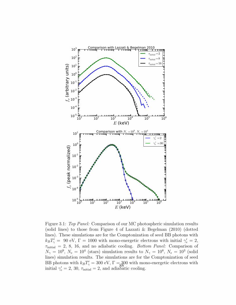
101 102 103 104 105 106

E (keV)

10-5

10-4

10-3

10-2

10-1

100

101

102

103

f ν (arbitrary units)

Comparison with Lazzati & Begelman 2010

τinitial=2

τinitial=8

τinitial=16

100 101 102 103 104 105 106

E (keV)

10-5

10-4

10-3

10-2

10-1

100

101

f ν (peak norm

alized)

Comparison with Nγ =109, Ne =104

γ ′e =2

γ ′e =30

Figure 3.1: Top Panel: Comparison of our MC photospheric simulation results(solid lines) to those from Figure 4 of Lazzati & Begelman (2010) (dottedlines). These simulations are for the Comptonization of seed BB photons withkBT

′γ = 90 eV, Γ = 1000 with mono-energetic electrons with initial γ′

e = 2,τinitial = 2, 8, 16, and no adiabatic cooling. Bottom Panel: Comparison ofNγ = 109, Ne = 104 (stars) simulation results to Nγ = 108, Ne = 103 (solidlines) simulation results. The simulations are for the Comptonization of seedBB photons with kBT

′γ = 300 eV, Γ = 300 with mono-energetic electrons with

initial γ′e = 2, 30, τinitial = 2, and adiabatic cooling.

88

those of Lazzati & Begelman (2010) (P-values) are 0.9999 for τinitial = 2, 0.9862

for τinitial = 8, and 0.9809 for τinitial = 16. This good agreement demonstrates

that our MC photospheric code is working properly.

We next perform a test to determine if 103 electrons are enough to

represent an electron distribution. If there are not enough electrons, the pho-

ton spectrum will look very noisy. Previous MC photospheric studies (Lazzati

& Begelman, 2010; Chhotray & Lazzati, 2015) found that 103 electrons are

enough to represent an electron distribution; however, their simulations were

performed for lower Nγ/Ne. To determine if 103 electrons are enough for our

Nγ/Ne = 105 simulations, we perform 2 simulations with Nγ = 109, Ne = 104

(10 times more photons and electrons) and compared them to simulation re-

sults with Nγ = 108, Ne = 103 in right panel of Figure 3.1 (we used the input

parameters described in Section 4.7.1.1 for mono-energetic electrons with ini-

tial γ′e = 2, 30 kBT

′γ = 300 eV, Γ = 300, and adiabatic cooling). From KS

tests, the probability that the two γ′e = 2 [γ′

e = 30] simulations are drawn

from the same distribution is 0.9999 [0.9999]. This good agreement explicitly

demonstrates that 103 electrons are enough for Nγ/Ne = 105 simulations.

3.4 Parameters Considered for MC Simulations with

Seed BB Photons

We now discuss the range of parameters we consider for our simula-

tions. The main input parameters that affect the output spectrum are kBT′γ

(determines the energy of the majority of the photons), γ′e (determines energy

89

in the electrons), and τinitial (determines the average number of scatterings

before a photon arrives at the photosphere). L determines the physical scales

of the system by determining Rinitial, Rphotosphere, n′e, and ℓ′mfp, but it does not

affect the number of scatterings or the shape of the spectrum. The main ef-

fect of Γ is to Doppler boost the photon spectrum to the observer frame. In

addition, Γ also determines the physical scales of the system by determining

Rinitial, Rphotosphere, n′e, and ℓ′mfp.

For our simulations, we considered kBT′γ = 30 eV, 100 eV, 300 eV. One

way the photon temperature can affect the output spectrum is through the

production of electron-positron pairs by photon annihilation, which would de-

crease (increase) the number of photons (electrons) in a simulation. However,

since the typical photon energies we are considering kBT′γ ∼ 30 eV−300 eV are

much less thanmec2, electron-positron pair production is expected to be unim-

portant and we neglect it for our simulations. Another more important effect

kBT′γ has on the simulation results is on the cooling of electrons. The pho-

tons in the jet-comoving frame are more energetic for larger kBT′γ and more

energetic photons will cool the electrons faster when they undergo multiple

scatterings.

γ′e is an important parameter since it determines the available energy

electrons have to transfer to photons. The smallest value we consider for γ′e

is 2. In the photospheric model, in order to avoid synchrotron cooling from

the magnetic field that is expected to be present in the jet, the synchrotron

emission is taken to be self-absorbed. The largest γ′e that can be considered

90

is found by setting the optical depth for synchrotron self-absorption equal to

1. Below, we calculate the largest γ′e allowed for MB and PL distributions of

electrons.

For a MB distribution distribution of electrons, the synchrotron self-

absorption optical depth τMBsyn is given by (Rybicki & Lightman, 1979; Lazzati

& Begelman, 2010)

τMBsyn =

106

(γ′e)

5ǫ1/2B (E ′

γ/1keV)2. (3.8)

In this equation, ǫB = UB/Urad, where UB (Urad) is the energy density in the

magnetic field (radiation) and we note that τMBsyn depends on the energy of the

photons in the comoving frame. Setting τMBsyn = 1, for ǫB ∼ 0.1 (magnetic field

subdominant to radiation) and E ′γ ∼ 300 eV (E ′

γ ∼ 100 eV) [E ′γ ∼ 30 eV], the

upper limit we find is γ′e ∼ 30 (γ′

e ∼ 50) [γ′e ∼ 80].

For a power-law distribution distribution of electrons, the synchrotron

self-absorption optical depth τPLsyn is given by (Wu et al., 2003; Gou et al., 2007)

τPLsyn =e

B′

(

(p− 1)(p+ 2)

(γ′1)

−(p−1) − (γ′2)

−(p−1)

)

×

2√6π3/2

9(γ′

2)−(p+4)exp(−1)σ−1

T . (3.9)

In this equation, γ′1 (γ′

2) is the electron Lorentz factor where the power-law

begins (ends) and B′ is the magnetic field in the jet-comoving frame. From the

expressions UB = (B′)2/(8π) and Urad = arad(T′γ)

4, B′ = (8πǫBarad)1/2(T ′

γ)2.

Setting τPLsyn = 1, taking γ′1 = 2, p = 2.4, and B′ corresponding to ǫB = 0.1

and kBT′γ = 300 eV (kBT

′γ = 100 eV) [kBT

′γ = 30 eV], the upper limit we

91

kBT ′

γ Mono-Energetic MB PL Distribution

30 eV γ′

e = 2, 30, 80kBT ′

e(γad,el−1)mec2

= (2-1), (80-1) γ′

e,1 = 2, γ′

e,2 = 80, p = 2.4

100 eV γ′

e = 2, 30, 50kBT ′

e(γad,el−1)mec2

= (2-1), (50-1) γ′

e,1 = 2, γ′

e,2 = 50, p = 2.4

300 eV γ′

e = 2, 10, 30kBT ′

e(γad,el−1)mec2

= (2-1), (30-1) γ′

e,1 = 2, γ′

e,2 = 30, p = 2.4

Table 3.1: γ′e values we consider for our simulations for each value of kBT

′γ and

the 3 different electron distributions we consider. For the MB distribution, wegive the value of kBT

′e = (γad,el−1)(γ′

e−1)mec2, where γad,el = (4γ′

e+1)/(3γ′e)

is the electron adiabatic index, since kBT′e measures the kinetic energy of the

electrons.

found for γ′2 is γ′

2 ∼ 30 (γ′2 ∼ 50) [γ′

2 ∼ 80]. Thus, for both a MB distribution

and a PL distribution, the maximum γ′e we can consider for kBT

′γ = 300 eV

(kBT′γ = 100 eV) [kBT

′γ = 30 eV] is ∼ 30 (∼ 50) [∼ 80]. A summary of the

values we considered for γ′e for each value of kBT

′γ is given in Table 3.1.

τinitial affects the shape of the spectrum since it determines the average

number of scatterings a photon experiences before escaping the photosphere.

The average number of scatterings for a photon is ∼ 2τinitial (Begue et al.,

2013), not ∼ (τinitial)2, since as the GRB relativistic outflow moves outward,

n′e decreases as R

2 (Equation 3.5). For our simulations, we considered τinitial =

2, 8, 16.

Lastly, since Nγ ≫ Ne for our simulations, the electrons rapidly cool by

IC scatterings and then the electrons no longer have much energy to transfer

to the photons. Thus, we also considered electron re-heating. At a given

τinitial, the total number of scatterings expected is ∼ 2τinitialNγ. To re-heat

the electrons, we first specify the number of re-heating events Nrh we choose

to consider. Then, after (2τinitialNγ)/(Nrh + 1) scatterings, we re-heat the

92

electrons to the same distribution that they were initialized to (we divide by

Nrh + 1 since the total number of heating events is the initial heating event

plus Nrh events). We adopt this methodology to have the re-heating events

evenly spaced within the total number of scatterings.

3.5 Simulation Results for Comptonization of Seed BB

Spectrum

In this section, we first show our results for one dissipation event, where

electrons are only accelerated once at the start of the simulation. Then, we

consider electron re-heating, where the electrons are re-accelerated back to

their initial distribution Nrh times.

3.5.1 Simulation Results for One Dissipation Event

In Figure 3.2, we show simulations for τinitial = 2, the three values

we considered for kBT′γ , and mono-energetic electrons with the values of γ′

e

shown in Table 3.1. As the reader many have noticed in Figure 3.1, the most

striking feature of the output spectrum is the sharp drop in fν by ∼ 2 orders

of magnitude after the peak energy, Epk. Unlike previous studies for Nγ/Ne =

1 − 104, our results for Nγ/Ne = 105 do not show a power-law immediately

after the peak energy. After the drop in fν , the simulations with γ′e = 2 in the

three panels continue to decline rapidly. On the other hand, the simulations

with γ′e ∼ 10 − 80 in each panel display a power-law for ∼ 2 − 3 decades in

energy before declining rapidly again. The highest energy the photons near the

93

100 101 102 103 104 105 106 107

E (keV)

10-5

10-4

10-3

10-2

10-1

100

101

f ν (peak

norm

aliz

ed)

Mono-Energetic Electrons, τinitial=2, kB T′γ =300 eV, Different γ ′

e

γ ′e =2

γ ′e =10

γ ′e =30

100 101 102 103 104 105 106 107

E (keV)

10-5

10-4

10-3

10-2

10-1

100

101

f ν (peak

norm

aliz

ed)


e

γ ′e =2

γ ′e =30

γ ′e =50

100 101 102 103 104 105 106 107

E (keV)

10-5

10-4

10-3

10-2

10-1

100

101

f ν (peak

norm

aliz

ed)


e

γ ′e =2

γ ′e =30

γ ′e =80

Figure 3.2: Top-Left panel: Simulation results for the Comptonization of seedBB photons with kBT

′γ = 300 eV, Γ = 300 with mono-energetic electrons with

initial γ′e = 2, 10, 30 and τinitial = 2. Top-Right panel: Same as Top-Left panel

for kBT′γ = 100 eV, Γ = 300 and mono energetic electrons with initial γ′

e = 2,30, 50. Bottom-Left panel: Same as Top-Left panel for kBT

′γ = 30 eV, Γ = 300

and mono energetic electrons with initial γ′e = 2, 30, 80.

94

BB peak can attain after one scattering is ∼ 4× (100 eV)Γ(γ′e)

2 ∼ 105 keV for

γ′e ∼ 50. Once the photons reach these energies, IC scattering is highly Klein-

Nishina (KN) suppressed, leading to an exponential decay in the spectrum for

higher energies.

In Figure 3.3, we show simulation results for τinitial = 2, the three

values we considered for kBT′γ, and the largest γ′

e we considered for each dis-

tribution in Table 3.1. In each panel, the PL distribution simulations display

the least broadened spectrum. This is due to the fact that the PL distribution

contains the least energetic electrons among these three distributions. The

mono-energetic and MB electron distribution simulations show similar results

since the two distributions are similar; the MB distribution has an average

γ′e very close to the γ′

e value we consider for the mono-energetic electrons.

After the sharp drop in fν in each panel, all the simulations display a single

power-law spectrum for ∼ 3 decades in energy.

In Figure 3.4, we show simulation results for τinitial = 2, 8, 16, the three

values of kBT′γ we considered, and MB electrons with the largest value we

considered for γ′e (see Table 3.1). In addition, in each panel, we also plot the

energy spectrum fν = ENE of the kinetic energies of the electrons at the end

of each simulation in the observer frame, i.e. mec2(γe − 1)Γ. Increasing τinitial

has two effects on the output spectrum: decreasing the number of photons

at higher energies and increasing the broadening of the spectrum. For larger

τinitial, the additional scatterings allow for the high-energy photons to transfer

energy back to the electrons. The increase in broadening of the spectrum from

95

100 101 102 103 104 105 106 107

E (keV)

10-5

10-4

10-3

10-2

10-1

100

101

f ν (peak norm

alized)

Different Electron Distributions, kB T ′γ =300 eV, τinitial=2

kB T ′e =(γad,el−1)(30−1)me c

2

γ ′e =30

γ ′e,1=2, γ ′

e,2=30, p=2.4

100 101 102 103 104 105 106 107

E (keV)

10-5

10-4

10-3

10-2

10-1

100

101

f ν (peak norm

alized)



2

γ ′e =50

γ ′e,1=2, γ ′

e,2=50, p=2.4

100 101 102 103 104 105 106 107

E (keV)

10-5

10-4

10-3

10-2

10-1

100

101

f ν (peak norm

alized)



2

γ ′e =80

γ ′e,1=2, γ ′

e,2=80, p=2.4


′γ = 300 eV, Γ = 300 with electrons following MB, mono

energetic, and PL distributions, and τinitial = 2. For each distribution, weconsidered the largest value of γ′

e we can consider for kBT′γ = 300 eV (see

discussion in Section 4.7.1.2 and Table 3.1). Top-Right panel: Same as Top-

Left panel but with kBT′γ = 100 eV, Γ = 300. Bottom-Left panel: Same as as

Top-Left panel but with kBT′γ = 30 eV, Γ = 300.

96

100 101 102 103 104 105 106 107

E (keV)

10-5

10-4

10-3

10-2

10-1

100

101

f ν (peak norm

alized)

kB T′e =(γad,el−1)(30−1)me c

2 , kB T′γ =300 eV, Different τinitial

τinitial=2

τinitial=8

τinitial=16

100 101 102 103 104 105 106 107

E (keV)

10-5

10-4

10-3

10-2

10-1

100

101

f ν (peak norm

alized)



τinitial=2

τinitial=8

τinitial=16

100 101 102 103 104 105 106 107

E (keV)

10-5

10-4

10-3

10-2

10-1

100

101

f ν (peak norm

alized)



τinitial=2

τinitial=8

τinitial=16


′γ = 300 eV, Γ = 300 with MB electrons with initial γ′

e ∼30 and τinitial = 2, 8 16. The photon (electron) spectra are represented bysolid (dotted) lines. For both the photons and the electrons, we are plottingtheir energy spectrum fν = ENE. The photon spectra are peak normalizedand the electron spectra are shifted down by a factor of 10 for each τinitial tobetter see if there is any change as τinitial becomes larger. Top-Right panel:

Same as Top-Left panel, but with kBT′γ = 100 eV, Γ = 300 and MB electrons

with initial γ′e ∼ 50. Bottom-Left panel: Same as Top-Left panel, but with

kBT′γ = 30 eV, Γ = 300 and MB electrons with initial γ′

e ∼ 80.

97

kBT′γ = 300 eV (Top-Left Panel) to kBT

′γ = 30 eV (Bottom-Left Panel) is due

to a couple of effects: 1. the larger γ′e considered for kBT

′γ = 30 eV allows for

the electrons to transfer more energy to the photons. 2. for kBT′γ = 30 eV,

the photons have lower energy in the jet-comoving frame, and thus, cool the

electrons more slowly, allowing for more photons to be upscattered to higher

energies. In each panel, the simulations with larger τinitial have a lower peak-

energy due to the adiabatic cooling of photons. In the top-left panel, the three

simulations show a sharp drop in fν by ∼ 2 orders of magnitude above the

peak energy. In the top-right panel, the τinitial = 8, 16 almost show a power-law

above the peak-energy, but the spectrum still declines rapidly. Fitting a power-

law to the τinitial = 8, 16 simulations, we find a steep spectrum fν ∝ ν−2. In

the bottom-left panel, the τinitial = 8, 16 simulations show a power-law above

the peak-energy, with a fν ∝ ν−1.2 spectrum, in agreement with the Band

function.

The electron distributions at the end of all the simulations display a

Maxwell-Boltzmann distribution. In each panel, as τinitial increases, the elec-

tron distributions become narrower and the electron temperature decreases.

This is due to the fact that the additional scatterings allow for the electrons

to transfer more energy to the photons.

In summary, we searched a wide parameter space for the photospheric

process in Figures 3.2-3.4. In Figure 3.2, for τinitial = 2, there is a sharp drop

in fν above the peak-energy by ∼ 2 orders of magnitude for all the photon

temperatures and γ′e values we considered. In Figure 3.3, we determined that

98

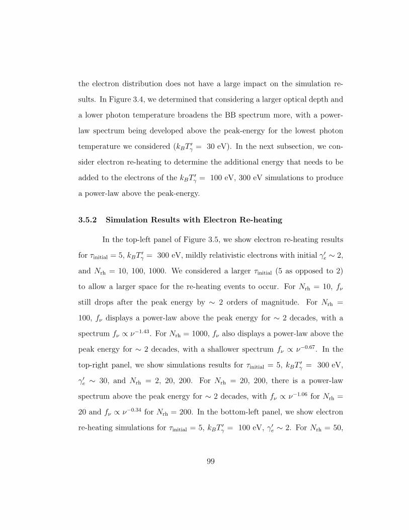
the electron distribution does not have a large impact on the simulation re-

sults. In Figure 3.4, we determined that considering a larger optical depth and

a lower photon temperature broadens the BB spectrum more, with a power-

law spectrum being developed above the peak-energy for the lowest photon

temperature we considered (kBT′γ = 30 eV). In the next subsection, we con-

sider electron re-heating to determine the additional energy that needs to be

added to the electrons of the kBT′γ = 100 eV, 300 eV simulations to produce

a power-law above the peak-energy.

3.5.2 Simulation Results with Electron Re-heating

In the top-left panel of Figure 3.5, we show electron re-heating results

for τinitial = 5, kBT′γ = 300 eV, mildly relativistic electrons with initial γ′

e ∼ 2,

and Nrh = 10, 100, 1000. We considered a larger τinitial (5 as opposed to 2)

to allow a larger space for the re-heating events to occur. For Nrh = 10, fν

still drops after the peak energy by ∼ 2 orders of magnitude. For Nrh =

100, fν displays a power-law above the peak energy for ∼ 2 decades, with a

spectrum fν ∝ ν−1.43. For Nrh = 1000, fν also displays a power-law above the

peak energy for ∼ 2 decades, with a shallower spectrum fν ∝ ν−0.67. In the

top-right panel, we show simulations results for τinitial = 5, kBT′γ = 300 eV,

γ′e ∼ 30, and Nrh = 2, 20, 200. For Nrh = 20, 200, there is a power-law

spectrum above the peak energy for ∼ 2 decades, with fν ∝ ν−1.06 for Nrh =

20 and fν ∝ ν−0.34 for Nrh = 200. In the bottom-left panel, we show electron

re-heating simulations for τinitial = 5, kBT′γ = 100 eV, γ′

e ∼ 2. For Nrh = 50,

99

Nrh=10

Nrh=100

Nrh=1000

10-1 100 101 102 103 104 105 106

E (keV)

10-5

10-4

10-3

10-2

10-1

100

101

f ν (peak norm

alized)

Re-heating, kB T′γ =300 eV, kB T

′e =(γad,el−1)(2−1)me c

2 , τinitial=5

Nrh=2

Nrh=20

Nrh=200

10-1 100 101 102 103 104 105 106

E (keV)

10-5

10-4

10-3

10-2

10-1

100

101

f ν (peak norm

alized)


′e =(γad,el−1)(30−1)me c

2 , τinitial=5

Nrh=5

Nrh=50

Nrh=500

10-1 100 101 102 103 104 105 106

E (keV)

10-5

10-4

10-3

10-2

10-1

100

101

f ν (peak norm

alized)


′e =(γad,el−1)(2−1)me c

2 , τinitial=5

Nrh=0

Nrh=5

Nrh=50

10-1 100 101 102 103 104 105 106

E (keV)

10-5

10-4

10-3

10-2

10-1

100

101f ν (peak norm

alized)


′e =(γad,el−1)(50−1)me c

2 , τinitial=5

Figure 3.5: Top-left Panel: Simulation results for the Comptonization of seedBB photons with kBT

′γ = 300 eV, Γ = 300 with mildly relativistic electrons

with initial γ′e ∼ 2, τinitial = 5, and Nrh = 10, 100, 1000 electron re-heating

events. Top-right Panel: Same as top-left panel, but with γ′e ∼ 30 and Nrh =

2, 20, 200 electron re-heating events. Bottom-left Panel: Simulation resultsfor the Comptonization of seed BB photons with kBT

′γ = 100 eV, Γ = 300

with mildly relativistic electrons with initial γ′e ∼ 2, τinitial = 5, and Nrh = 5,

50, 500 electron re-heating events. bottom-right Panel: Same as top-left panel,but with γ′

e ∼ 50 and Nrh = 0, 5, 50 electron re-heating events.

100

500, there is a power-law spectrum above the peak energy for∼ 2 decades, with

fν ∝ ν−1.41 for Nrh = 50 and fν ∝ ν−0.59 for Nrh = 500. In the bottom-right

panel, we show electron re-heating simulations for τinitial = 5, kBT′γ = 100 eV,

γ′e ∼ 50. For Nrh = 5, 50, there is a power-law spectrum above the peak energy

for ∼ 2 decades, with fν ∝ ν−1.00 for Nrh = 5 and fν ∝ ν−0.44 for Nrh = 50.

In summary, the main finding of considering electron re-heating is that

there is only a fν ∝ ν−1 spectrum above the peak energy if a specific number if

electron re-heating events are considered. If too few electron re-heating events

are considered, there is still a sharp drop in fν after the peak energy and if

too many electron re-heating events are considered, the high-energy spectrum

will be shallower than fν ∝ ν−1.

3.6 Discussion of Results for the Comptonization of BB

Photons

In this section, we first discuss an energy requirement the electrons must

satisfy to have enough energy to transfer to the photons to produce a power-law

spectrum above the peak-energy. This energy requirement is a necessary, but

not a sufficient condition, to explain the production of a power-law spectrum

above the peak-energy. To give a more detailed explanation for the simulation

results, we calculate the number of photons upscattered to higher energies in

a simulation and compare this to the number of photons needed to be upscat-

tered to produce a power-law spectrum. After this calculation, we discuss the

interpretation for the drop in fν by ∼ 2 orders of magnitude, immediately after

101

the peak energy Epk, for the simulations with kBT′γ ∼ 30 eV − 300 eV, one

heating event, and τinitial = 2. We also discuss the interpretation of the simu-

lations with kBT′γ = 30 eV and τinitial 8, 16, which show a power-law spectrum

above Epk. We then apply this interpretation to the electron re-heating simu-

lations with kBT′γ = 100 eV, 300 eV to estimate how many electron reheating

events it takes to produce a power-law spectrum above Epk. Lastly, we discuss

the dependence of the simulation results on the photon to electron ratio.

3.6.1 Energy Requirement for Power-Law Spectrum

In order to produce a power-law spectrum above the peak-energy, the

electrons must have enough energy to transfer to the photons so they can

populate a high-energy tail. A power-law spectrum can develop if the energy

of a significant fraction of the photons near the BB peak-energy, ∼ 1/2, can

be increased by a factor ∼ 2. Taking the number of photons near the BB peak

to be ∼ Nγ (most of the photons are near the peak), the energy requirement

the electrons must satisfy is

Nemec2γ′

e & 2(Nγ/2)kBT′γ (3.10)

When considering kBT′γ = 300 eV and kBT

′γ = 100 eV, we considered γ′

e ∼ 30

and γ′e ∼ 50, respectively. For these two cases, for Nγ/Ne ∼ 105 (as observed

for the GRB prompt emission), the electrons just meet the energy requirement,

making the production of a power-law spectrum difficult (in agreement with

the results presented in the top two panels of Figure3.4). When considering

kBT′γ = 30 eV, we considered γ′

e ∼ 80. For this case, the energy in the electrons

102

is ∼ 10 larger than the energy that needs to be transferred to the photons.

Thus, the electrons have enough energy to transfer to the photons to produce

a power-law spectrum for this case, in agreement with the results presented in

the bottom-left panel of Figure3.4.

We now discuss a more detailed calculation to understand and interpret

out simulation results.

3.6.2 Discussion of MC Simulation Results with One Heating Event

To understand our MC simulation results, we need to determine the

number of photons that need to be upscattered to energies larger than Epk

to produce a power-law spectrum. We refer to this quantity as Npl. We then

compare Npl to the total number of photons that are upscattered to energies

larger than Epk in a MC simulation, which is given by the number of electrons

in a simulation, Ne, multiplied by NComp. NComp represent the number of

scatterings it takes to cool an electron to a critical γ′e at which Comptonization

is no longer important. Thus, in order to produce a power-law above Epk, we

need the condition

NeNComp & Npl (3.11)

to be satisfied. We now estimate Npl and NComp for our MC simulations.

103

3.6.2.1 Estimating Npl

The number of photons in some bin with energy E, denoted as NE, is

given by

NE =Npk

Epk

(

E

Epk

)−β−1

. (3.12)

In this equation, Npk is the number of photons at Epk and the spectral index

β is defined in the fν sense, i.e. fν ∝ ν−β. To determine the total number of

photons needed to produce a power-law above Epk, we integrate NEdE (sum

over all the bins) from Epk to infinity:

Npl =

∞∫

E′pk

Npk

Epk

(

E

Epk

)−β−1

dE =Npk

β. (3.13)

For the prompt emission, the typical high-energy spectral index is β = 1.2

(Preece et al., 2000). Thus, we approximate Npl ∼ Npk. Since the majority

of the photons in a simulation are near the peak of the BB spectrum, we

approximate Npl ∼ Npk ∼ Nγ. With this result for Npl, we can rewrite the

condition to produce a power-law above Epk (Equation 3.11) in terms of the

photon to electron ratio (Nγ/Ne):

NComp &Nγ

Ne∼ 1× 105. (3.14)

In the above expression, we used Nγ/Ne = 105 for our MC simulations (Equa-

tion 3.2).

104

3.6.2.2 Condition for electron γ′e at which Comptonization is no

longer important

The Compton-Y parameter determines if the energy of a photon will

change significantly after undergoing multiple scatterings with electrons in

a optically thick medium. The expression for the Compton-Y parameter is

(Rybicki & Lightman, 1979)

Y = 2τinitial ×max

[

4kBT′e

mec2,4

3[(γ′

e)2 − 1]

]

, (3.15)

where 2τinitial is the average number of scatterings for each photon (Begue

et al., 2013) and the average fractional change of energy for a photon after a

scattering event is either 4kBT′e/mec

2 (for mildly-relativistic or sub-relativistic

electrons) or (4/3)[(γ′e)

2 − 1] (for relativistic electrons), depending on the γ′e

of the electron. We take the transition from relativistic to mildly-relativistic

speeds to occur at γ′e = 2.

The condition Compton-Y & 1 needs to be satisfied for Comptonization

to be important. At the start of our MC simulations, Compton-Y > 1 since

both 2τinitial (we consider τinitial ≥ 2) and max[4kBT′e/mec

2, (4/3)([γ′e]2−1)] (we

consider γ′e ≥ 2) are larger than one. However, as the simulations proceed,

since Nγ ≫ Ne, the electrons may cool to a point where Comptonization is no

longer important. The critical condition at which Comptonization is no longer

important is given by

2τinitial ×4kBT

′e

mec2∼ 1. (3.16)

Entering kBT′e ∼ mec

2(γ′e,Comp−1), where γ′

e,Comp is the electron Lorentz factor

105

at which Comptonization is no longer important, we find

γe,Comp = 1 +1

8τinitial. (3.17)

Thus, γe,Comp = 1.06 for τinitial = 2 and γe,Comp = 1.008 for τinitial = 16. With

the value for γe,Comp, we can now estimate NComp.

3.6.2.3 Estimating NComp

The final γ′e (γ′

e,f) of an electron after a scattering event can be found

from energy conservation (see Appendix B.5), which is given by

γ′e,f =

E ′γ,i − E ′

γ,f +mec2γ′

e,i

mec2, (3.18)

where E ′γ,i [E

′γ,f ] is the photon energy before [after] the scattering event and

γ′e,i is the electron Lorentz factor before the scattering event. As we discussed

above, the average change of energy for a photon after a scattering event

depends on whether γ′e > 2 or γ′

e < 2 (Rybicki & Lightman, 1979):

E ′γ,f −E ′

γ,i =4

3[(γ′

e,i)2 − 1]E ′

γ,i , for γ′e,i > 2 (3.19)

E ′γ,f −E ′

γ,i =4kBT

′e

mec2E ′

γ,i , for γ′e,i < 2. (3.20)

Substituting these expressions for E ′γ,f −E ′

γ,i into Equation 3.18, we can solve

for the change in electron γ′e after a scattering event in terms of E ′

γ,i and γ′e,i:

γ′e,f − γ′

e,i = −4E ′

γ,i

3mec2[(γ′

e,i)2 − 1] , for γ′

e,i > 2 (3.21)

γ′e,f − γ′

e,i = −4E ′

γ,i

mec2[γ′

e,i − 1] , for γ′e,i < 2. (3.22)

106

In Equation 3.22, for γ′e,i < 2, we used kBT

′e ∼ mec

2(γ′e,i − 1) for the electron

temperature. If we define the change in electron γ′e per scattering as dγ′

e/dN ,

we can re-write Equation 3.21 and Equation 3.22 in differential form:

dγ′e

dN= −

4E ′γ

3mec2[(γ′

e)2 − 1] , for γ′

e > 2 (3.23)

dγ′e

dN= −

4E ′γ

mec2[γ′

e − 1] , for γ′e < 2. (3.24)

In the above expressions, E ′γ represents the energy of the photon in the jet-

comoving frame before the scattering event. Solving these differential equa-

tions, we find

NCool,Rel =3mec

2

8E ′γ

ln

[

(γ′e,MR + 1)(γ′

e,i − 1)

(γ′e,MR − 1)(γ′

e,i + 1)

]

, for γ′e,i > 2 (3.25)

NCool,MR =mec

2

4E ′γ

ln

[

(γ′e,i − 1)

(γ′e,Comp − 1)

]

, for γ′e,i ≤ 2. (3.26)

In Equation 3.25, NCool,Rel represents the number of scatterings it takes to cool

a relativistic electron with γ′e,i > 2 to γ′

e,MR = 2. After an electron cools below

γ′e,MR = 2, NCool,MR represents the number of scatterings it takes to cool a

mildly-relativistic (MR) electron from γ′e,i ≤ 2 to γ′

e,Comp.

For our simulations, we considered γ′e,i ≥ 2. If we consider γ′

e,i > 2, to

compute NComp, we first need to compute the number of scatterings it takes

to cool an electron to γ′e,MR = 2 (Equation 3.25). Then, we need to compute

the number of scattering it takes to cool an electron with γ′e,i = 2 to γ′

e,Comp

(Equation 3.26). Thus, the number of scatterings it takes to cool a relativistic

electron to γ′e,Comp (defined as NComp,Rel) is

NComp,Rel = NCool,Rel(γ′e,i > 2) +NCool,MR(γ

′e,i = 2). (3.27)

107

NCool,MR(γ′e,i = 2) NCool,MR(γ

′e,i = 2) NCool,Rel(γ

′e,i > 2)

τinitial = 2 τinitial = 16

kBT′γ =30 eV ∼ 104 ∼ 2× 104 ∼ 7× 103 for γe,i = 80

kBT′γ =100 eV ∼ 3× 103 ∼ 6× 103 ∼ 2× 103 for γe,i = 50

kBT′γ =300 eV ∼ 103 ∼ 2× 103 ∼ 7× 102 for γe,i = 30

Table 3.2: Values of NComp for the simulations we presented in Figures 3.2-3.4. NComp,MR and NComp,Rel were calculated with Equation 3.26 and Equation3.27, respectively.

On the other hand, for a mildly-relativistic electron with γ′e,i ≤ 2, the num-

ber of scatterings it takes to cool an electron from γ′e,i to γ′

e,Comp (defined as

NComp,MR) is simply found by computing NCool,MR (Equation 3.26). We give a

summary of the values of NComp for the simulations we presented in Figures

3.2-3.4 in Table 3.2. When using Equation 3.25 and 3.26 to calculate NCool,Rel

and NCool,MR, we assume E ′γ ∼ kBT

′γ , i.e. that the electrons cool mostly by

scattering photons near the BB peak. This is not a bad approximation since

most of the photons are near the BB peak.

3.6.2.4 Interpretation of MC Simulation Results with One Heating

Event

From the estimates we provided in Table 3.2 for NComp at τinitial = 2,

for kBT′γ ∼ 30 eV − 300 eV and initial γ′

e ∼ 2− 80, NComp ∼ 2000− 10000 <

(Nγ/Ne) (Equation 3.14). Thus, not enough photons are upscattered to en-

ergies above Epk to produce a power-law spectrum. The fraction of photons

that can be upscattered to energies larger than Epk is given by

Fraction of upscattered photons =NeNComp

Nγ=

NComp

(Nγ/Ne), (3.28)

108

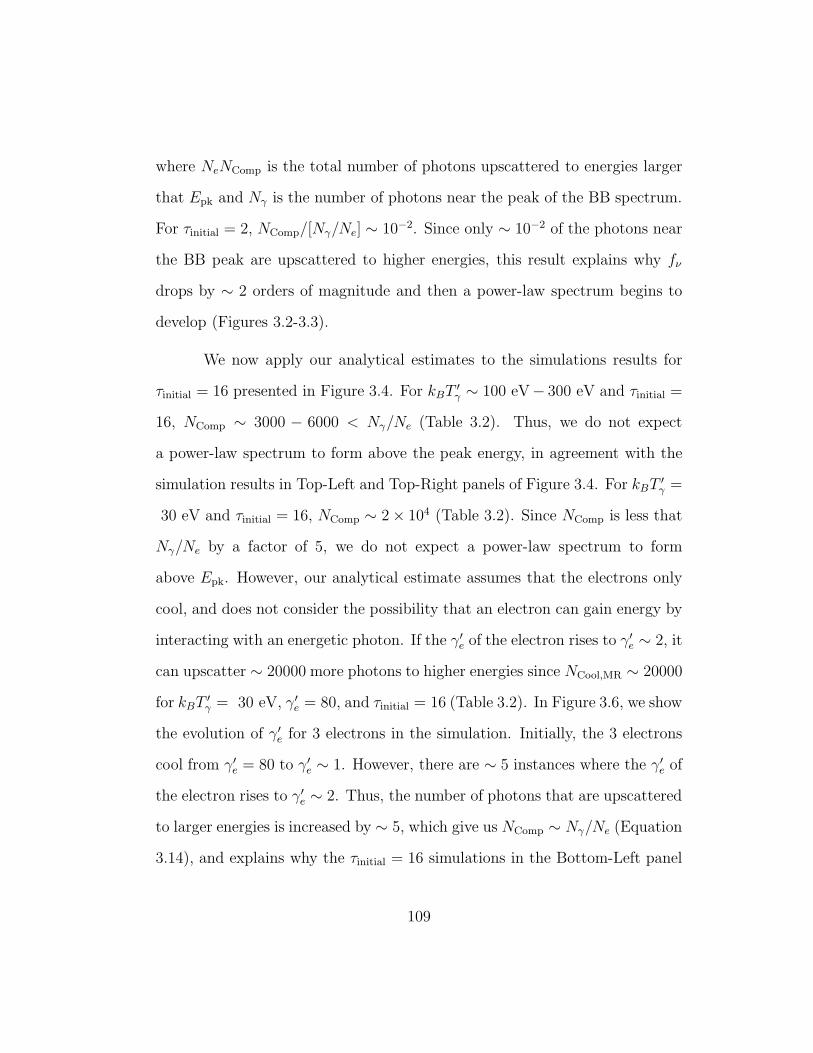
where NeNComp is the total number of photons upscattered to energies larger

that Epk and Nγ is the number of photons near the peak of the BB spectrum.

For τinitial = 2, NComp/[Nγ/Ne] ∼ 10−2. Since only ∼ 10−2 of the photons near

the BB peak are upscattered to higher energies, this result explains why fν

drops by ∼ 2 orders of magnitude and then a power-law spectrum begins to

develop (Figures 3.2-3.3).

We now apply our analytical estimates to the simulations results for

τinitial = 16 presented in Figure 3.4. For kBT′γ ∼ 100 eV− 300 eV and τinitial =

16, NComp ∼ 3000 − 6000 < Nγ/Ne (Table 3.2). Thus, we do not expect

a power-law spectrum to form above the peak energy, in agreement with the

simulation results in Top-Left and Top-Right panels of Figure 3.4. For kBT′γ =

30 eV and τinitial = 16, NComp ∼ 2× 104 (Table 3.2). Since NComp is less that

Nγ/Ne by a factor of 5, we do not expect a power-law spectrum to form

above Epk. However, our analytical estimate assumes that the electrons only

cool, and does not consider the possibility that an electron can gain energy by

interacting with an energetic photon. If the γ′e of the electron rises to γ′

e ∼ 2, it

can upscatter ∼ 20000 more photons to higher energies since NCool,MR ∼ 20000

for kBT′γ = 30 eV, γ′

e = 80, and τinitial = 16 (Table 3.2). In Figure 3.6, we show

the evolution of γ′e for 3 electrons in the simulation. Initially, the 3 electrons

cool from γ′e = 80 to γ′

e ∼ 1. However, there are ∼ 5 instances where the γ′e of

the electron rises to γ′e ∼ 2. Thus, the number of photons that are upscattered

to larger energies is increased by ∼ 5, which give us NComp ∼ Nγ/Ne (Equation

3.14), and explains why the τinitial = 16 simulations in the Bottom-Left panel

109

100 101 102 103 104 105 106

Number of scatterings

100

101

102

103

104

Electron γ

′ e


2 , kB T′γ =30 eV, τinitial=16

Electron 1: 100×γ ′eElectron 2: 10×γ ′eElectron 3: γ ′e

Figure 3.6: Evolution of γ′e for 3 electrons from the τinitial = 16 simulations

shown in the Bottom-Left panel of Figure 3.4. The γ′e of the electrons were

offset by a factor of 10 to better see the evolution of γ′e for each electron. Each

of the spikes for γ′e represents an episode when an electron interacts with an

energetic photon, causing the energy of the electron to increase by a largefactor.

110

of Figure 3.4 show a power-law spectrum above Epk.

3.6.3 Discussion of MC Simulation Results with Electron Reheat-

ing

In this subsection, we use the results for Npl and NComp to understand

the electron re-heating simulations with kBT′γ = 100 eV - 300 eV presented

in Figure 3.5. We estimate Nrh,min, the minimum number of re-heating events

needed to produce a power-law spectrum above Epk.

3.6.3.1 Estimating Nrh,min

With Nrh electron re-heating events, the number of photons that can

be upscattered to higher energies is ∼ NrhNeNComp. Nrh,min is found by the

condition where just enough photons are upscattered to energies larger than

Epk to produce a power-law spectrum, i.e.

Nrh,minNeNComp = Npl. (3.29)

Using the result Npl ∼ Nγ , the condition for Nrh,min can be re-written in terms

of the photon to electron ratio:

Nrh,min ∼Nγ/Ne

NComp. (3.30)

For kBT′γ = 300 eV and γ′

e,i ∼ 2 − 30, NComp ∼ 2000 − 3000 (Table 3.2);

thus we estimate Nrh,min ∼ 30 − 50. Nrh,min is within a factor of a few of the

simulations in the top panels of Figure 3.5, which show a power-law above

the peak-energy for Nrh ∼ 20 − 100. For kBT′γ = 100 eV and γ′

e,i ∼ 2 − 50,

111

NComp ∼ 5000− 8000 (Table 3.2); thus we estimate Nrh,min ∼ 10− 20. Nrh,min

is within a factor of a few of the simulations in the bottom panels of Figure

3.5, which show a power-law above the peak-energy for Nrh ∼ 5− 50.

3.6.4 Dependence of Comptonization of Seed BB Simulation Re-

sults on Nγ/Ne

In this subsection, we perform a quick set of simulations at τinitial = 2

to explore the dependence of the simulation results on Nγ/Ne. In the left panel

(right panel) of Figure 3.7, we show simulations results for kBT′γ = 300 eV,

Γ = 300, Nγ/Ne = 102, 103, 104, 105, τinitial = 2, and mono-energetic electrons

with initial γ′e = 2 (γ′

e = 30). For Nγ/Ne = 102 we considered Ne = 106, for

Nγ/Ne = 103 we considered Ne = 105, etc. This was done to keep Nγ = 108 so

that the simulation output spectrum can have more photons and thus a higher

signal to noise. For initial γ′e = 2 (left panel of Figure 3.7), the spectrum

shows a sharp drop above the peak energy for Nγ/Ne = 104. For Nγ/Ne =

103, the spectrum shows a power-law with fν ∝ ν−1.60 and for Nγ/Ne = 102

the spectrum also shows a power-law with fν ∝ ν−0.80. For initial γ′e = 30

(right panel of Figure 3.7), the spectrum shows a sharp drop above the peak

energy for Nγ/Ne = 104. For Nγ/Ne = 103, there is a power-law spectrum

fν ∝ ν−0.70 and for Nγ/Ne = 102 the spectrum is very shallow. The difference

in the simulation results with Nγ/Ne can be understood from a energetics

perspective. Equation 3.10, the minimum energy the electrons must have to

transfer to the photons to produce a power-law spectrum, can be rewritten in

112

Nγ /Ne =105

Nγ /Ne =104

Nγ /Ne =103

Nγ /Ne =102

100 101 102 103 104 105 106 107

E (keV)

10-6

10-5

10-4

10-3

10-2

10-1

100

101

f ν (peak norm

aliz

ed)

Different Nγ/Ne, τinitial=2, kBT′γ =300eV, Mono-Energetic Elec, γ ′

e =2

Nγ /Ne =105

Nγ /Ne =104

Nγ /Ne =103

Nγ /Ne =102

100 101 102 103 104 105 106 107

E (keV)

10-6

10-5

10-4

10-3

10-2

10-1

100

101

f ν (peak norm

aliz

ed)

Different Nγ/Ne, τinitial=2, kBT′γ =300eV, Mono-Energetic Elec, γ ′

e =30

Figure 3.7: Top Panel: Simulation results for the Comptonization of seedBB photons with kBT

′γ = 300 eV, Γ = 300 with mildly relativistic electrons

with initial γ′e = 2, four different values for the photon to electron ratio,

and τinitial = 2. Bottom Panel: Same as Left Panel but with mono-energeticelectrons with initial γ′

e = 30.

113

terms of the photon to electron ratio:

mec2γ′

e

Nγ/Ne

& kBT′γ . (3.31)

Thus, for a fixed kBT′γ , an increase in Nγ/Ne makes it more difficult to produce

a power-law spectrum above the peak-energy, as demonstrated in both panels

of Figure 3.7. These results highlight the strong dependence of the simulation

results on Nγ/Ne and the importance of performing simulations with Nγ/Ne =

105.

Lastly, we note that Lazzati & Begelman (2010) also show a couple

of simulation results for mono-energetic electrons with γ′e = 2, τinitial = 2,

and Nγ/Ne = 104 in their Figures 5-6. Their results for Nγ/Ne = 104 also

show a significant dip above the peak energy by a factor ∼ 50. However, our

simulation results in the left panel of Figure 3.7 for γ′e = 2 with Nγ/Ne = 104

display a drop in fν above Epk by a factor ∼ 100. This difference in the dip in

fν above the peak energy can be explained by the fact that Lazzati & Begelman

(2010) considered a value for kBT′γ smaller than the kBT

′γ value we considered

by a factor of 2. Since NCool,MR ∝ 1/E ′γ (Equation 3.26), a smaller value for

kBT′γ by a factor of 2 implies that twice as many photons will be upscattered to

larger energies (Equation 3.28). Thus, the Nγ/Ne = 104 presented in Lazzati

& Begelman (2010) are consistent with our analytical estimates and with our

simulation results for Nγ/Ne = 104.

114

3.7 Comptonization of Synchrotron fν ∝ ν−1/2 Spectrum

In this section, we consider a fν ∝ ν−1/2 seed spectrum, instead of BB

seed spectrum, as expected for electrons producing synchrotron emission in the

fast cooling regime (Ghisellini et al., 2000). We study how Comptonization

modifies this spectrum with our MC photospheric code. In the next subsection,

we describe the input parameters for these simulations.

3.7.1 Input Parameters for Simulations with Seed fν ∝ ν−1/2 Spec-

trum

For most of the input parameters, we considered the same values as

those we considered for the Comptonization of a seed BB spectrum (discussed

in Section 4.7.1.1). We considered Γ = 300, L = 1052 ergs/sec, τinitial = 2, 5,

8, 16, Ne = 103, Nγ = 108 to reach Nγ/Ne = 105, and Ncollect = Nγ/3. For

the fν ∝ ν−1/2 seed spectrum, the input parameters are E ′1,γ and E ′

2,γ , the

energy where the fν ∝ ν−1/2 spectrum begins and ends, respectively, in the

jet-comoving frame. Thus, in the observer frame, the fν ∝ ν−1/2 spectrum

begins and ends at E1,γ = ΓE ′1,γ and E2,γ = ΓE ′

2,γ. As we will discuss in the

next subsection, the effect of Comptonizing a fν ∝ ν−1/2 spectrum is to flatten

it to fν ∝ ν0, reminiscent of the low-energy spectrum of the prompt emission.

Since the observed fν ∝ ν0 spectrum for the prompt emission extends from .

10 keV to Epk = 300 keV, we considered values of E1,γ < 10 keV and E2,γ =

Epk.Thus, we considered E ′1,γ = 10 eV/Γ, 300 eV/Γ and E ′

2,γ = 300 keV/Γ.

For the electron distribution, we considered MB electrons with kBT′e ∼ (20 −

115

1)mec2, ∼ (200 − 1)mec

2, and ∼ (2000 − 1)mec2. Since the seed spectrum

was only flattened to fν ∝ ν0 for kBT′e ∼ (2000 − 1)mec

2, we only display

the simulation results for this value of kBT′e. Lastly, we note that we do not

consider electron re-heating, i.e. the electrons are only accelerated once at the

start of the simulations.

3.7.2 Simulation Results for Comptonization of fν ∝ ν−1/2 Seed

Spectrum

In the left panel (right panel) of Figure 3.8, we show the results for

the Comptonization of a seed fν ∝ ν−1/2 spectrum with E1,γ = 10 eV (E1,γ =

300 eV), E2,γ = 300 keV, MB electrons with kBT′e ∼ (2000 − 1)mec

2, and

τinitial = 2, 5, 8, 16. In addition, in both panels, we also plot the energy

spectrum fν = ENE of the kinetic energies of the electrons in the observer

frame, i.e. mec2(γe−1)Γ, at the end of each simulation. We will first discuss the

results for the electron distributions. At the end of the τinitial = 2 simulations,

the electron distributions peak at kBT′e ∼ 100 keV (in the jet-comoving frame)

for both panels. As τinitial increases, kBT′e doesn’t change by much; at the end of

the τinitial = 16 simulation kBT′e ∼ 50 keV for both panels. On the other hand,

the photon spectrum changes significantly as τinitial increases. For both panels,

at the end of the τinitial = 2 simulations, most of the photons are still near E1,γ ,

where most of the photons in the seed spectrum are initially present. However,

as τinitial increases, more and more photons begin to be upscattered to energies

∼ 104 keV. For both panels, at the end of the τinitial = 16, the spectrum is flat

from ∼ 1 keV to ∼ 104 keV. After ∼ 104 keV, the spectrum declines rapidly

116

10-4 10-3 10-2 10-1 100 101 102 103 104 105 106

E (keV)

10-5

10-4

10-3

10-2

10-1

100

101

f ν (peak norm

alized)

(E γ1 )′ =10−2 eV, (E γ

2 )′ =300 eV, kB T′e =(γad,el−1)(2000−1)me c

2

Seed fν∝ν−1/2

τinitial=2

τinitial=5

τinitial=8

τinitial=16

10-2 10-1 100 101 102 103 104 105 106

E (keV)

10-5

10-4

10-3

10-2

10-1

100

101

f ν (peak norm

alized)

(E γ1 )′ =0.3 eV, (E γ

2 )′ =300 eV, kB T ′e =(γad,el−1)(2000−1)me c

2

Seed fν∝ν−1/2

τinitial=2

τinitial=5

τinitial=8

τinitial=16

Figure 3.8: Top Panel: Simulation results for the Comptonization of a seedfν ∝ ν−1/2 spectrum (E ′

1,γ = 10−2 eV, E ′2,γ = 300 eV) with MB electrons

with kBT′e ∼ (2000− 1)mec

2 and τinitial = 2, 5, 8, 16. Bottom Panel: Same asLeft Panel, but with E1,γ = 0.3 eV.

117

for all of the simulations. After the rapid decline, there are a significant number

of photons with energies & 105 keV for all of the simulations. These photons

remain at these energies since they are highly Klein-Nishina suppressed and

cannot transfer their energy back to the electrons.

We now discuss the basic interpretation for the flattening of the spec-

trum as τinitial increases. From Equation 3.17, for τinitial = 16, the γ′e at which

Comptonization is no longer important is γe,Comp = 1.008. At the end of

the τinitial = 16 simulations, kBT′e ∼ 50 keV. Using kBT

′e ∼ mec

2(γe − 1),

γ′e ∼ 1.1 > γe,Comp. Thus, Comptonization is still important for the τinitial = 16

simulations and the photons are still gaining energy from the electrons. The

photons will gain energy from the electrons until they reach the energy of the

electrons. For the seed fν ∝ ν−1/2 spectrum, initially there are more photons

at lower energies near E1,γ . However, as τinitial increases, the additional scat-

terings allow for more photons at lower energies to be upscattered to higher

energies and they also allow for more photons to reach the energy of the elec-

trons. The spectrum flattens because more photons are being removed from

lower energies and being placed at high energies near the energy of the elec-

trons. If we considered τinitial > 16, if Compton-Y remains greater than 1,

eventually all the photons will be upscattered to energies close to the energy

of the electrons. The photon spectrum will no longer look flat, but will instead

be peaked at the energy of the electrons.

Lastly, we note that although the simulation output spectra for τinitial =

16 in both panels of Figure 3.8 are very similar to the low-energy spectrum for

118

the prompt emission, these simulation results cannot explain it. The spectrum

peaks at the energy of the electrons, which have an energy ∼ 50 keV in the

jet-comoving frame and thus an energy ∼ 50 keV × 300 ∼ 104 keV in the

observer frame (Γ = 300). In order for the spectrum to break at ∼ 300 keV

in the observer frame, the electrons would need to have an energy ∼ 1 keV in

the jet-comoving frame.

3.8 Conclusions

In this work, we presented our methodology for our MC photospheric

code and our simulation results for a wide parameter space with a realistic

photon to electron ratio Nγ/Ne = 105, as expected for the GRB prompt emis-

sion. Our goal was to determine if the photospheric process can explain the

observed high-energy spectrum fν ∝ ν−1.2 of the prompt emission. For these

simulations, we considered the Comptonization of a seed BB spectrum. If

electron re-heating is not considered, we determined that considering both

low photon temperatures and large optical depths ∼ 10 − 20 is best for pro-

ducing a power-law spectrum above the BB peak energy for the following two

reasons: 1. low temperature photons cool electrons more slowly, allowing more

photons to be upscattered to higher energies. 2. At larger optical depths, the

average number of scatterings a photon experiences is larger, allowing for more

photons to be upscattered to higher energies. On the other hand, the output

spectrum for the cases we considered with higher photon temperatures and low

optical depths display a sharp drop in fν above the peak energy by ∼ 2 orders

119

of magnitude. These cases require additional energy in the electrons and we

demonstrated that if we consider electron re-heating, a power-law spectrum

above the peak-energy can be produced.

One issue with the simulations with a low photon temperature and a

large optical depth is that it may be difficult to match the peak-energy of the

prompt emission since adiabatic cooling of photons decreases the BB peak-

energy by a large factor for large optical depths. Thus, considering electron

re-heating near the photosphere with a large photon temperature (∼ 100 keV

in the observer frame) may be the best solution for explaining the prompt

emissions observations with the photospheric model.

We also performed photospheric simulations for different values ofNγ/Ne

and demonstrated that the simulation results have a strong dependence on the

photon to electron ratio. This result highlights the important of performing

realistic photospheric simulations with Nγ/Ne = 105.

In addition, we also used our MC photospheric code to study how

Comptonization modifies a fν ∝ ν−1/2 seed spectrum, as expected for syn-

chrotron when electrons are in the fast cooling regime. For large optical

depths, the effect is to flatten the spectrum to fν ∝ ν0, reminiscent of the

low-energy spectrum of the Band function. However, these simulation results

cannot explain the low-energy spectrum of the prompt emission since the sim-

ulation output spectrum peaks at ∼ 104 keV, much larger than the ∼ 300 keV

peak energy of the prompt emission.

120

Chapter 4

Constraining The X-ray Flare Mechanism

with Optical Observations

4.1 Abstract

We study Gamma-Ray Burst (GRB) X-ray flares with coincident opti-

cal observations during the X-ray flare. For 8 X-ray flares, we determined that

the X-ray flare peak-flux, extrapolated to the optical band with a fν ∝ ν1/3

optically-thin Synchrotron/SSC (Synchrotron Self-Compton) spectrum, over-

produces the observed optical flux by a factor & 2. Thus, the synchrotron

and SSC processes require a self-absorption break between the optical and the

X-ray band to be compatible with the optical observations. We performed a

parameter space search for synchrotron, SSC, synchrotron from a Poynting

jet, and Monte Carlo simulations for the photospheric process to determine

if these mechanisms can explain the flare observations. Synchrotron and SSC

face problems: the variability time of the synchrotron solutions is much shorter

than the observed flare variability time and the synchrotron component of SSC

over-produces the observed optical flux. Synchrotron from a Poynting jet and

the Photospheric process both have a wide parameter space that explains the

flare observations. Thus, a Poynting jet and a baryonic jet can both explain

the X-ray flare observations, with the photospheric process being the best

121

candidate for a baryonic jet.

4.2 Introduction

One of the most puzzling observations provided by the Swift satellite

(Gehrels et al., 2004a) is the observation of erratic episodes of rebrightenings

in the X-ray light curve following the prompt gamma-ray emission, known as

X-ray flares (Burrows et al., 2005a). X-ray flares have been detected for ∼ 33%

of long GRBs and for ∼ 13% of short GRBs (Chincarini et al., 2007, 2010;

Bernardini et al., 2011; Margutti et al., 2011). During a X-ray flare episode,

the flux increases by a factor ∼ 1 − 103 and there are many cases where a

GRB is seen to display multiple X-ray flares. The rapid rise time of the flux,

with ∆t/tpk ∼ 0.1, where ∆t is the duration of the flare and tpk is the time

when the flare peaks, rules out the external-forward shock as the mechanism

for X-ray flares (Lazzati & Perna, 2007). Thus, X-ray flares are believed to

be due to re-activation of the central engine after the prompt emission (King

et al., 2005; Perna et al., 2006; Proga & Zhang, 2006; Rosswog, 2007; Lee et al.,

2009; Dai et al., 2006b; Wang & Dai, 2013).

In addition to the open question on how to restart the central engine

to power X-ray flares, another key open question is, what is the X-ray flare

radiation mechanism? Detailed spectral studies of X-ray flares have revealed

that flares have similarities to prompt gamma-ray pulses (Butler & Kocevski,

2007a; Margutti et al., 2010; Sonbas et al., 2013). Thus, understanding the

X-ray flare radiation mechanism may help us understand the prompt radia-

122

tion mechanism, one of the long standing questions in the GRB field. One

of the main challenges for studying the X-ray flare mechanism is that ex-

cept in a few cases (Kruhler et al., 2009; Abdo et al., 2011; Li et al., 2012;

Swenson et al., 2013; Swenson & Roming, 2013), there is no signal associ-

ated with X-ray flares in other bands. In particular, it is surprising that no

signal associated with X-ray flares is detected in the optical band since the

UVOT (Ultra-Violet/Optical Telescope, Roming et al. (2005)) on-board the

Swift satellite and many rapid-response ground based optical facilities have

taken high quality optical observations during X-ray flare episodes (e.g. Cenko

et al., 2009; Rykoff et al., 2009; Uehara et al., 2010; Gorbovskoy et al., 2012;

Kopac et al., 2013; Zaninoni et al., 2013; Melandri et al., 2014).

In this work, we focus on bursts that have optical observations coinci-

dent with the flare to constrain the X-ray flare radiation mechanism. To use

the coincident optical observations, we take the peak-flux of the X-ray flare

and extrapolate it to the optical band and compare it to the observed optical

flux. Taking the X-ray flare emission to peak in the X-ray band, the optically-

thin synchrotron and SSC (Synchrotron Self-Compton) processes both predict

fν ∝ ν1/3 below the peak, where fν is the flux per unit frequency ν. For 8 X-

ray flares, we found that the predicted flux for optically thin synchrotron/SSC

over-predicts the observed optical flux by a factor & 2. Thus, in order to

not over-produce the observed optical flux, synchrotron and SSC require a

self-absorption break between the optical and the X-ray band. We perform

a parameter space search to determine if the synchrotron and SSC processes

123

can produce a self-absorption break between the optical and X-ray band. In

addition, we also perform a parameter space search for synchrotron emission

from a magnetized jet and we perform Monte Carlo simulations of the pho-

tospheric process to determine if these processes can explain the X-ray flare

observations.

This manuscript is organized as follows. In Section 4.3, we describe

the extrapolation of the X-ray flare peak flux to the optical band in more

detail and we present our sample of 8 flares that require a self-absorption

break between the optical band and the X-ray band (observations are shown

in Appendix C). In Section 4.4, Section 4.5, and Section 4.6 we discuss the

results for our parameter space search for synchrotron, SSC, and synchrotron

from a Poynting jet, respectively. In Section 4.7, we discuss the results of our

Monte Carlo simulations for the photospheric process. Lastly, in Section 4.8,

we discuss our conclusions.

4.3 X-ray Flares with Self-Absorption break between

Optical and X-ray band

4.3.1 Extrapolating X-ray flare peak-flux to Optical band

We performed a literature search for X-ray flares that have a measured

spectrum, optical observations coincident with the X-ray flare episode, and a

measured redshift. A number of studies have used observations from Swift’s

XRT (X-ray Telescope, Burrows et al. 2005b), which has an observing band

from 0.3-10 keV, to determine the spectrum for X-ray flares with high signal

124

to noise (e.g. Falcone et al., 2006; Pagani et al., 2006; Goad et al., 2007; Morris

et al., 2007; Butler & Kocevski, 2007a; Falcone et al., 2007; Margutti et al.,

2010; Chincarini et al., 2010). The two models that best fit the X-ray flare

spectrum are the Band function (Band et al., 1993) and a single-power law

(Falcone et al., 2007), with most flares being better fit by a single power-law.

In addition, some studies have found a photospheric component in the X-ray

flare spectrum (Larsson et al., 2011; Friis & Watson, 2013). The spectrum of

the 8 X-ray flares in our sample were better fit by either a Band function or a

single power-law.

To extrapolate the X-ray flare emission to the optical band, we ob-

tained the peak specific flux for each X-ray flare at 10 keV, f10keV, from the

XRT lightcurves in Evans et al. (2010)1. For the X-ray flares with a Band

function spectrum, we used the spectral index above Epk (peak energy of

Band function) to extrapolate f10keV to Epk. Below Epk, we used a fν ∝ ν1/3

spectrum to extrapolate to the optical band2. Defining the extrapolated flux

to the optical band as f2eV,pred and defining the spectral index above Epk in

the fν sense as βB (fν ∝ ν−βB), f2eV,pred = f10keV(Epk/10keV)−βB(2eV/Epk)1/3.

For the X-ray flares with a single power-law spectrum, we used the observed

spectral index, β, to extrapolate f10keV to 0.3 keV, the low-energy end of

the XRT band. The observed spectrum of the X-ray flare likely extends be-

low 0.3 keV, but to be conservative in the extrapolation to the optical band,

1http://www.swift.ac.uk/burst analyser/2Most X-ray flares in our sample have Epk ∼ 1keV and the energy range 0.3 keV - Epk

is too narrow to determine the low-energy spectral index accurately.

125

we assumed fν ∝ ν1/3 between 2 eV and 0.3 keV. For these X-ray flares,

f2eV,pred = f10keV(0.3keV/10keV)−β(2eV/0.3keV)1/3.

4.3.2 Sample of X-ray flares

In Appendix C, we show the optical and X-ray light curves for the 8

flares in our sample. In Table 4.1, we show some of the observational properties

for these 8 X-ray flares: trise (rise time of flare), tpk (time when flare peaks), z

(redshift of burst), dL28 (luminosity distance in units of 1028 cm), LX,50 (peak

luminosity of the flare radiated in X-rays in units of 1050 ergs/sec), and f2eV,corr

(optical flux at 2 eV, corrected for both Galactic extinction and host galaxy

extinction). We also give the reference information for the optical data and

the X-ray flare spectrum.

4.3.3 Flare Properties Used for Parameter Space Search

The flares in our sample can be divided into three categories: flares with

a Band functions spectrum, flares with a single power-law fν ∝ ν−0.5 (GRB

060714 and GRB 080310), and flares with a single power-law spectrum steeper

than fν ∝ ν−0.5 (GRB 051117A and GRB 081008). In order to describe the

properties of all the flares in our sample. we will perform the parameter space

search for 4 flares in our sample: GRB 060904B and GRB 061121 (both with

Band function spectrum), GRB 080310, and GRB 081008.

126

4.4 Synchrotron Parameter Space Search

We now discuss our strategy for searching the 5D synchrotron parame-

ter space to determine if there are solutions with νa between the optical band

and X-ray band.

4.4.1 Methodology for Synchrotron Parameter Space Search

The 5 parameters that describe a synchrotron source are (Kumar &

McMahon, 2008; Beniamini & Piran, 2013): the radius of emission R, the mag-

netic field strength B, the number of emitting electrons Ne, the bulk Lorentz

factor of the source Γ, and taking the radiating electrons to follow a power-law

distribution dNe/dγe ∝ γ−pe (γe is the Lorentz factor of the electrons and p is a

constant known as the electron-index), the fifth parameter is γi, the minimum

Lorentz factor electrons must have to follow this power-law distribution. To

search this 5D parameter space, we allow the following 5 parameters to be

free: Γ, the flare variability time ∆t, and the electron Lorentz factors γi, γa,

and γc, corresponding to electrons radiating photons with frequencies νi, νa,

and νc respectively, where νc is the cooling frequency. In addition, we also

calculate the Compton-Y parameter to include inverse Compton (IC) cooling

of electrons. By letting Γ, ∆t, γi, γa, γc be free, we already know 2 of the 5 pa-

rameters that describe a synchrotron source (Γ and γi). We now describe how

we use Γ, ∆t, γi, γa, γc to compute R, B, Ne and the Compton-Y parameter.

With Γ and ∆t, we can compute the radius of emission with the ex-

127

pression

R = 2c∆tΓ2(1 + z)−1, (4.1)

where c is the speed of light. Next, we use γc to compute B in terms of

Compton-Y . The expression for γc, the electron Lorentz factor for electrons

cooling on a dynamical timescale tdyn = [R(1 + z)]/(2cΓ2) (in the observer

frame), is

γc =6πmec

σTt−1dynΓ

−1B−2(1 + z)×

(1 + Y )−1 γa < γc

(χ(γc/γa) + Y )−1 γc < γa.(4.2)

In this equation, σT is the Thomson cross-section. When γc < γa, the source

cannot cool by synchrotron since the synchrotron emission is self-absorbed

(Granot et al., 2000; Panaitescu & Meszaros, 2000; Gao et al., 2013); thus,

the cooling of electrons is dominated by IC scattering. In this regime, we

calculate γc as in Panaitescu & Meszaros (2000). When γc < γa, the (1+Y )−1

term is modified by an optical depth term: γc ∝ (χ(γc/γa) + Y )−1 , where

χ = 1− exp(−γc/γa) (Panaitescu & Meszaros, 2000). With Equation 4.2, we

can solve for B in terms of Compton-Y :

B =

(

6πmec

σT

)1/2

(tdyn)−1/2Γ−1/2(1 + z)1/2γ−1/2

c ×

(1 + Y )−1/2

(χ(γc/γa) + Y )−1/2 .

(4.3)

Next, we compute Ne in terms of Compton-Y . Ne enters into the

synchrotron expressions from fνp, the peak flux of the fν spectrum:

fνp =

√3e3

4πmec2BNeΓd

−2L (1 + z). (4.4)

128

To solve for Ne, we enter fνp (Equation 4.4) into the expression for νa. The

expression for νa depends on the ordering of γi, γa, γc; we list each expression

for νa below (Gou et al., 2007; Shen & Zhang, 2009; Zhao et al., 2010):

νa =

(

12me

)35f

35νpd

65LR

− 65Γ

35 (1 + z)−

95γ

− 35

i ν− 1

5i γa < γi < γc

(

e8πm3

ec

)1

p+4f

2p+4νp d

4p+4

L R− 4p+4Γ

3p+4 (1 + z)−

7p+4ν

p−1p+4

i B1

p+4 γi < γa < γc(

12me

)35

f35νpd

65LR

− 65Γ

35 (1 + z)−

95γ

− 35

c ν− 1

5c γa < γc < γi

(

e8πm3

ec

)16f

13νpd

23LR

− 23Γ

12 (1 + z)−

76B

16 ν

16c γc < γa < γi

(

e8πm3

ec

)1

p+5f

2p+5νp

(

dLR

)4

p+5 Γ3

p+5 (1 + z)−7p+5B

1p+5ν

p−1p+5

i ν1

p+5c max(γi, γc) < γa

(4.5)

When solving for Ne with Equation 4.5, we also enter

νi = [e/(2πmec)]Bγ2i Γ(1 + z)−1, νa = [e/(2πmec)]Bγ2

aΓ(1 + z)−1,

and νc = [e/(2πmec)]Bγ2cΓ(1 + z)−1. Simplifying this result, Ne in terms of

Compton-Y is given by

Ne =

(

2√3πe

)

R2B ×

γ5/3i γ

10/3a γa < γi < γc

γ−(p−1)i γp+4

a γi < γa < γc

γ5/3c γ

10/3a γa < γc < γa

γ−1c γ6

a γc < γa < γi

γ−1c γ

−(p−1)i γp+5

a max(γi, γc) < γa

(4.6)

In these expressions, the dependence of Ne on Compton-Y comes from B

(Equation 4.3). With Ne in terms of Compton-Y , we can now solve for

Compton-Y .

129

The Compton-Y parameter is given by the expression

Y =4

3

(

σTNe

4πR2

)

∫

Neγ2eNγe dγe

Ne, (4.7)

where τe = σTNe/(4πR2) is the optical depth to electron-scattering. The term

∫

Neγ2eNγe dγe/Ne represents the 2nd moment of the electron distribution di-

vided by the total number of electrons, which can be determined from the

electron distribution. Taking p > 2, the expressions for the electron distri-

bution for the slow cooling (γi < γc) and the fast cooling (γc < γi) cases are

given by

Nγe =

(p− 1)γ−(p−1)i γ−p

e Ne γi < γe < γc

(p− 1)γ−(p−1)i γcγ

−p−1e Ne γc < γe

(4.8)

Nγe =

γcγ−2e Ne γc < γe < γi

γ−(p−1)i γcγ

−p−1e Ne γi < γe

(4.9)

Taking the 2nd moment of the electron distributions, we find

∫

Neγ2eNγe dγe

Ne=

(p− 1)γ(p−1)i

[

γ3−pc

(3−p)(p−2)− γ3−p

i

(3−p)

]

γi < γc

γc(γi − γc) +γcγip−2

γc < γi. (4.10)

Entering the values for∫

Neγ2eNγe dγe/Ne into Equation 4.7, entering B (Equa-

tion 4.3) into the Ne (Equation 4.6), and entering Ne into Equation 4.7, Equa-

tion 4.7 now only depends on the Compton-Y parameter and on our free

parameter Γ, ∆t, γi, γa, γc. This allows us to solve Equation 4.7 numerically

to determine Compton-Y . With Compton-Y , we can now find B (Equation

4.3) and Ne (Equation 4.6). Thus, we now have all the parameters that de-

scribe a synchrotron source and we use them to compute νa (Equation 4.5) to

determine if it is between the optical and X-ray band.

130

4.4.2 Free Parameter Ranges for 5D Parameter Space Search

We consider a very broad space for the 5D parameter space search.

The range we consider for each parameter is: 2 < Γ < 1000, 10−4 sec < ∆t <

102 sec, 2 < γa < 106, 2 < γi < 106, and 2 < γc < 106.

4.4.3 Constraints for Valid Synchrotron Solutions

In addition to producing νa between the optical and X-ray band, we

also require that synchrotron solutions match the observed spectral index, the

observed X-ray flux, and have an optical flux below the observed optical flux.

Above the peak energy of the fν spectrum, the synchrotron spectrum is either

fν ∝ ν−p/2 (satisfied when max(νa, νi, νc) < ν), fν ∝ ν−(p−1)/2 (satisfied when

max(νa, νi) < ν < νc), or fν ∝ ν−0.5 (satisfied when max(νa, νc) < ν < νi)

(Granot & Sari, 2002). Thus, for three of the four flares we consider for our

parameter space search (Section 4.3.3), which have a spectrum fν ∝ ν−1.47,

fν ∝ ν−1.4, fν ∝ ν−1.51 (GRB 060904B, 061121, 081008, respectively), we

consider both fν ∝ ν−p/2 and fν ∝ ν−(p−1)/2 when fitting their spectrum,

with p determined from the spectral index. For GRB 080310, the fν ∝ ν−0.5

segments are used to fit the observed fν ∝ ν−0.476 spectrum. When β = 0.5,

the spectral index cannot be used to determine p. From Table 4.1, a typical

spectral index for the flares in our sample is β = 1.4. Thus, we consider both

p = 2.8 and p = 3.8 for GRB 080310.

For the flares that are better fit by a Band function, we require fνp

to match fEpk= f10keV(10 keV/Epk)

−βB within a factor of 2. We also require

131

the peak energy of the fν synchrotron spectrum, νi, νa, or νc, depending on

the ordering of γi, γa, or γc, to match Epk within a factor of 2. On the other

hand, for the flares with a single power-law spectrum, the peak energy lies

between 2 eV and 0.3 keV. For these flares, we extrapolate the flux at fνp

to 0.3 keV and require it to match f0.3keV = f10keV(0.3 keV/10 keV)−β within

a factor of 2. For the parameter space determined to have νa between the

optical and the X-ray band, we use the synchrotron spectrum to find the flux

at 2 eV. Below the peak energy, fν ∝ ν1/3 for νa < ν < min(νi, νc), fν ∝ ν2

for ν < min(νa, νi), and fν ∝ ν5/2 for νi < ν < νa (Granot & Sari, 2002).

We require the synchrotron flux at 2 eV to be below the observed optical flux

f2eV,cor.

In addition to describing the optical and X-ray observations, we also re-

quire that the IC component does not violate energy requirements. The energy

radiated in X-rays for the flares in our sample is ∼ 1051 − 1052 ergs. If Y > 1,

the energy in the IC component is larger than the energy in the synchrotron

component by a factor of Y . In addition, if the 1st IC scattering is not Klein-

Nishina (KN) suppressed, there will be a 2nd IC scattering, which will carry

an energy larger than the synchrotron component by a factor Y 2. Multiple IC

scatterings will continue, each carrying an energy larger than the previous IC

scattering by a factor of Y , until the IC emission is KN suppressed, i.e. the

condition νsyn(4γ2e)

Nγe > mec2Γ, where N refers to the Nth IC scattering and

νsyn refers to the peak energy of the fν synchrotron spectrum.

If Y < 1, we do not consider additional IC scatterings. If Y > 1, we

132

consider a synchrotron solution to be valid if Y < 1000 (to keep the energy

budget below ∼ 1054− 1055 ergs) and the 2nd IC scattering is KN suppressed.

If the 2nd IC scattering is not KN suppressed, we include a 2nd IC scattering

in our methodology by adding a Y 2 term to the γc equation (Zhao et al., 2010):

γc =6πmec

σTt−1dynΓ

−1B−2(1 + z)×

(1 + Y + Y 2)−1 γa < γc

(χ(γc/γa) + Y + Y 2)−1 γc < γa.(4.11)

Thus, B in terms of Compton-Y is given by

B =

(

6πmec

σT

)1/2

(tdyn)−1/2Γ−1/2(1+z)1/2γ−1/2

c ×

(1 + Y + Y 2)−1/2

(χ(γc/γa) + Y + Y 2)−1/2

(4.12)

In this equation, the top case is for γa < γc, the bottom case is for γc < γa.

With this expression for B, Ne is still given by Equation 4.6. We then solve

Equation 4.7 for Compton-Y , which allows us to determine B, Ne, and the

synchrotron frequencies νi, νa, νc. We consider a solution with a 2nd IC

scattering to be valid if Y 2 < 1000 and the 3rd IC scattering is KN suppressed.

We do not include a 3rd IC scattering since for a νsyn ∼ 100 eV - 1 keV and

γe ∼ 10− 100, it is likely KN suppressed.

4.4.4 Results for Synchrotron Parameter Space Search

In Figure 4.1, we show the parameter space of allowed solutions that

satisfy the constraints discussed in Section 4.4.3 for the 4 flares we consider for

our parameter space search (Section 4.3.3). We were only able to find valid so-

lutions for the flares with a single power-law spectrum. None of the parameter

133

Figure 4.1: Parameter space of acceptable solutions for synchrotron for theX-ray flares in our sample.

space for the flares with a Band function spectrum produces νa > 2 eV. This is

due to the fact that to fit the X-ray observations, fνp = f10keV(Epk/10 keV)−β,

with Epk ∼ 1 keV for the Band function flares and Epk is a free parameter

between 2 eV and 0.3 keV for the flares with a single power-law spectrum.

The larger fνp for the single power-law flares requires more electrons, making

self-absorption stronger. In addition, the parameter space of valid synchrotron

solutions for the single power-law spectrum flares is unattractive since the al-

lowed variability time is ∼ 10−4 − 10−1 sec, much smaller than the typical

10-100 sec observed flare variability time. These findings make synchrotron

an unattractive mechanism to explain the X-ray flares observations for our

134

Figure 4.2: Allowed values for Compton-Y , EB, Ee, and Ep for the synchrotronparameter space search.

sample.

In Figure 4.2, we show the values of Compton-Y and the energy in

electrons (Ee), magnetic field (EB), and cold protons (Ep) for the solutions

that satisfy the synchrotron constraints. The energies were calculated with

the following expressions:

Ee = Nemec2γpΓ (4.13)

EB =1

6B2R3 (4.14)

Ep = Nemec2Γ, (4.15)

where γp is the electron Lorentz factor at the peak of the fν synchrotron

135

spectrum.

4.5 SSC Parameter Space Search

In this section, we discuss our strategy for searching the 5D SSC pa-

rameter space to determine if SSC can explain the observations of the X-ray

flares in our sample.

4.5.1 Methodology for SSC Parameter Space Search

The 5 parameters that describe a SSC source are also Γ, R, B, Ne, γi.

For the SSC parameter space search, we first calculate the seed synchrotron

photon field with the synchrotron methodology described in Section 4.4. Thus,

we continue to take Γ, ∆t, γi, γa, γc as free parameters. As with synchrotron,

we also consider multiple scatterings for SSC until the IC emission is KN

suppressed. In addition to including the 1st scattering and the 2nd scattering,

we also consider a 3rd IC scattering for SSC; to include it, we add a Y 3 term

to γc:

γc =6πmec

σT

t−1dynΓ

−1B−2(1 + z)×

(1 + Y + Y 2 + Y 3)−1 γa < γc

(χ(γc/γa) + Y + Y 2 + Y 3)−1 γc < γa.

(4.16)

Thus, B in terms of Compton-Y is given by

B =

√

6πmec

σT

(tdyn)−1/2Γ−1/2(1+z)1/2γ−1/2

c ×

(1 + Y + Y 2 + Y 3)−1/2

(χ(γc/γa) + Y + Y 2 + Y 3)−1/2

(4.17)

136

In this equation, the top case is for γa < γc, the bottom case is for γc < γa.

As before, with this expression for B, Ne is still given by Equation 4.6. We

then solve Equation 4.7 for Compton-Y , which allows us to determine B, Ne,

and the synchrotron frequencies νi, νa, νc. We then use the electron Lorentz

factors γi, γa, γc and νi, νa, νc to calculate the IC scattered frequencies. We

did not include a 4th IC scattering since it is likely KN suppressed.

For SSC, we require that νICa (IC scattered self absorption frequency)

is between the optical and X-ray band. The break frequencies for the SSC

spectrum are given in Table 4.2. In addition, as for synchrotron, we require

the SSC spectrum to be consistent with the X-ray and optical observations.

The peak specific flux of the SSC spectrum (f ICνp ) is given by

f ICνp = 3τefνp, (4.18)

where τe = (σTNe)/(4πR2) and fνp is the peak synchrotron flux (Equation

4.4). The major differences between the synchrotron and SSC spectrum are 1.

The number of break frequencies: If min(γi, γa, γc) 6= γa, there are only 2 break

frequencies in the SSC spectrum. 2. For max(γi, γa, γc) 6= γa, fν ∝ ν1 for ν <

νICa and when max(γi, γa, γc) = γa, fν ∝ ν1 for ν < νIC

a,1. In addition, above f ICνp ,

the SSC spectrum is slightly curved since the SSC spectrum is approximately

the synchrotron spectrum multiplied by a logarithmic (ln(ν)) term (Panaitescu

& Meszaros, 2000; Sari & Esin, 2001; Gao et al., 2013). However, we neglect

this slight curvature and approximate the SSC spectrum above f ICνp as power-

law segments. Thus, if max(γi, γa, γc) 6= γa, above the peak energy, the SSC

137

spectrum is either fν ∝ ν−p/2 (satisfied when max(νICa , νIC

i , νICc ) < ν), fν ∝

ν−(p−1)/2 (satisfied when max(νICa , νIC

i ) < ν < νICc ), or fν ∝ ν−0.5 (satisfied

when max(νICa , νIC

c ) < ν < νICi ) (Gao et al., 2013). When max(γi, γa, γc) = γa,

fν ∝ ν−p/2 for ν > νICa,2, fν ∝ ν−(p−1)/2 for νIC

a,1 < ν < νICa,2 and γi < γc < γa,

and fν ∝ ν−1/2 for νICa,1 < ν < νIC

a,2 and γc < γi < γa (Panaitescu & Meszaros,

2000).

4.5.2 Constraints for Valid SSC Solutions

To fit the observed spectral index, as with the synchrotron parameter

space search, we continue to consider both the fν ∝ ν−p/2 and fν ∝ ν−(p−1)/2

segments for GRBs 060904B, 061121, 081008 and the fν ∝ ν−0.5 segments for

GRB 080310 with both p = 2.8 and p = 3.8. To match the observed X-ray

flux, for the flares with a Band function, we require f ICνp to match fEpk

=

f10keV(10 keV/Epk)−βB within a factor of 2 and the SSC break frequency at

f ICνp to match Epk within a factor of 2. For the flares with a single power-

law spectrum, we extrapolate f ICνp to 0.3 keV and require it to match f0.3keV =

(0.3 kev/10 keV)−β within a factor of 2. For the solutions with νICa between the

optical and X-ray band, we also require that both the SSC and the synchrotron

flux at 2 eV are below the observed optical flux f2eV,cor. To find the SSC flux

below the peak energy, we use the SSC spectrum below the peak energy: for

max(γi, γa, γc) 6= γa, fν ∝ ν1/3 for νICa < ν < min(νIC

i , νICc ) and fν ∝ ν1 for

ν < νICa ; for max(γi, γa, γc) = γa fν ∝ ν1 for ν < νIC

a,1. The synchrotron photon

field usually peaks below the optical band. Thus, we use the synchrotron

138

segments above fνp to extrapolate fνp to 2 eV: fν ∝ ν−p/2, fν ∝ ν−(p−1)/2, and

fν ∝ ν−0.5.

Lastly, as with the synchrotron parameter space search, we also re-

quire that the IC emission from multiple IC scatterings not violate energy

constraints. For SSC, the 1st IC produces the ∼ 1051 − 1052 ergs of energy

observed for X-ray flares. If the 2nd IC scattering is not KN suppressed, for a

valid solution, we require Y 2 < 1000 and that the 3rd IC scattering is KN sup-

pressed. If the 3rd IC scattering is not suppressed, we require Y 3 < 1000 for a

valid synchrotron solution; we take the 4th IC scattering to be KN suppressed.

4.5.3 Results for SSC Parameter Space Search

For the 4 bursts we consider for our X-ray flare parameter space search

(Section 4.3.3), we found a very narrow parameter space of solutions for GRB

080310, which has an observed X-ray spectrum fν ∝ ν−1/2, and we found no

solutions for the other three bursts. The basic problem with SSC is that the

seed synchrotron field overproduces the observed flux at 2 eV. From Table

4.1, the X-ray flux at 0.3keV-1keV is ∼ 100 times larger than the observed

flux at 2 eV. Thus, in order to match the observed X-ray flare peak flux with

f ICνp = 3τefνp , the seed synchrotron flux will be larger than the observed optical

flux by a factor ∼ 100/(3τe). This large synchrotron flux overproduces the

observed optical flux by a large factor. Thus, we determine that SSC is not a

good mechanism to explain the X-ray flare observations. Lastly, we note that

Troja et al. (2015) performed a similar parameter space search for SSC and

139

they also determined that SSC cannot explain the X-ray flare observations.

4.6 Synchrotron from a Poynting Jet Parameter Space

Search

In this section, we consider synchrotron from a Poynting jet, where

the energy of the jet is carried primarily by magnetic fields. In a Poynting

model, magnetic reconnection is taken to dissipate the magnetic field and

the particles are accelerated in regions referred to as Particle Acceleration

Sites (PASs), associated with X-points. In these X-points, the magnetic field

lines reconnect and the electric field generated by reconnection is taken to

accelerate the electrons. These electrons then radiate synchrotron emission

while inside the PASs. Although the magnetic field in a PAS is strong, the

electrons will not cool significantly as long as the rate at which the electrons are

radiating energy is less than the rate at which the electrons gain energy through

magnetic reconnection. The time spent by electrons in PASs is unknown. Once

an electron leaves a PAS, it will cool by radiating synchrotron in the strong

magnetic field present in the jet. Multiple PASs are expected to be produced

in the jet by magnetic reconnection and the electrons can be re-accelerated by

entering another PAS.

A predictive model for radiation from a Poynting jet has not been

developed due to the poorly understood details of magnetic reconnection and

particle acceleration in magnetic reconnection regions. Recently, Kumar &

Crumley (2015) used global properties of the magnetic field and conservation

140

laws to understand the broad properties of radiation from a Poynting jet. In

this section, we apply the model presented in Kumar & Crumley (2015) to

X-ray flares.

4.6.1 Methodology for Poynting Jet Parameter Space Search

In a Poynting jet, the jet luminosity can be used to determine the

strength of the magnetic field in the jet, defined as B0 (B0 is measured in the

jet-comoving frame):

L = (B0)2Γ2R2c → B0 =

√

L/c

RΓ. (4.19)

In the PASs, although some of the magnetic field B0 is dissipated by magnetic

reconnection to produce an electric field, the magnetic field in PAS is still of

order B0 (Kumar & Crumley, 2015). Thus, by determining B0, we determine

the magnetic field inside PASs. To determine B0, we take L = 5LX , i.e. we

assume ∼ 20% efficiency in the conversion of jet energy to X-ray radiation

(values of LX in Table 4.1) and for R we use Equation 4.1. With the value for

B0, we can now perform a parameter space search for synchrotron emission

inside PASs. As in Section 4.4, we continue to take Γ, ∆t, γi, γc, and γa, as

free parameters. We neglect the IC cooling of electrons for the Poynting model

since the strong magnetic field in the Poynting jet leads to the synchrotron

power dominating over the IC power. To determine Ne, we continue to use

Equation 4.6, with B0 entered for B. We now have all the parameters that

describe a synchrotron source (Γ, R, B, γi, Ne), which allows us to use Equa-

tion 4.5 to calculate νa and determine if it is between the optical and X-ray

141

band. One last detail we note is the following: since electrons are expected

to remain hot, and not cool while inside PAS, we do not consider the cases

with strong synchrotron self-absorption, i.e. γc < γa. Thus, for the Poynting

model parameter space search, we only consider the regimes γa < γi < γc,

γi < γa < γc, and γa < γc < γi.

4.6.2 Constraints for Valid Poynting Solutions

As we described in Section 4.4.3, for a valid solution, in addition to

producing a νa between the optical and X-ray band, we also require that

solutions match the observed spectral index, the observed X-ray flux, and

produce an optical flux below the observed optical flux. Furthermore, for a

valid Poynting solution, we also require that the synchrotron emission from

inside PASs is larger than the synchrotron emission from outside PASs. The

ratio of the synchrotron flux from inside PASs to the synchrotron flux from

outside PASs, at the peak of the fν spectrum, is given by (Kumar & Crumley,

2015)

Rp =ξt′dyn

t′cool(γp). (4.20)

In this equation, ξt′dyn is the time electrons spend inside PASs (in the jet-

comoving frame) and t′cool(γp) = (6πmec)/(σTB20γp) is the synchrotron cooling

time (in the jet-comoving frame) for electrons radiating outside PASs and

γp = min(γi, γc). For the timescale electrons spend inside PAS, ξ is a free

parameter, which we take to be in the range 10−3 < ξ < 1 and t′dyn = R/(2cΓ).

Thus, a smaller ξ leads to electrons spending less time in PASs, which leads to

142

Figure 4.3: Parameter space of acceptable solutions for synchrotron radiationfrom a Poynting jet for the X-ray flares in our sample.

a smaller value for Rp. In order for the emission from inside PAS to dominate

over the emission from outside PAS, we enforce the condition Rp > 10 for

acceptable solutions for the Poynting model. Lastly, we note that we enforce

the conditions EB > Ee and EB > Ep so that the energy in the magnetic field

dominates over the energy in electrons and protons.

4.6.3 Results for Poynting Jet Parameter Space Search

In Figure 4.3 and Figure 4.4, we show the parameter space that satis-

fies the constraints discussed in Section 4.6.2 for the 4 flares we consider for

our parameter space search (Section 4.3.3). We were able to find solutions

143

Figure 4.4: Allowed values for ξ, EB, Ee, and Ep for our synchrotron emissionfrom a Poynting jet parameter space search. In the top-left panel, the blankspaces in between the horizontal lines are due to our grid size of 5 points perlog decade in ξ.

for both the flares that have a Band function spectrum and a single power-

law spectrum. The parameter space of the allowed solutions is very broad.

In particular, there are solutions for the flare variability time spanning from

10−4 sec to 102 sec, with ∼ 10 - 100 seconds being a typical time for flares. One

small drawback of the Poynting model is that studies on particle acceleration

in magnetic reconnection regions find p < 2, whereas we need either p = 2.8

or p = 3.8 to fit the observed X-ray flare spectrum. Otherwise, synchrotron

radiation from a Poynting jet is a good candidate to explain the radiation

144

mechanism of the flares in our sample.

4.7 Parameter Space Search for the Photospheric Pro-

cess

Another mechanism that has been studied in detail to explain the

prompt emission is the photospheric process (Thompson, 1994b; Ghisellini &

Celotti, 1999; Meszaros & Rees, 2000; Meszaros et al., 2002; Rees & Meszaros,

2005; Pe’er et al., 2006; Thompson et al., 2007; Pe’er, 2008; Giannios, 2008; Be-

loborodov, 2010; Lazzati & Begelman, 2010; Beloborodov, 2011; Toma et al.,

2011; Pe’er & Ryde, 2011; Mizuta et al., 2011; Lundman et al., 2013; Lazzati

et al., 2013; Ruffini et al., 2013; Begue et al., 2013; Deng & Zhang, 2014; Ito

et al., 2014; Begue & Iyyani, 2014). The basic picture of the photospheric

process is as follows. Photons are assumed to be produced below the photo-

sphere. At an optical depth τ ∼ few, a dissipation event is assumed to occur,

which accelerates electrons to mildly relativistic or relativistic speeds 3. In the

photospheric model, the average energy of the photons is taken to be much

smaller than the average energy of the electrons. Thus, while the outflow is

still optically thick, the photons and electrons undergo multiple scatterings

(Comptonization) and the photons gain energy from the electrons until their

energy reaches the average electron energy. Although not a necessary condi-

3The dissipation events discussed in the literature for the photospheric process are mag-netic reconnection (Thompson, 1994b; Giannios & Spruit, 2005; Giannios, 2006, 2012) andinternal shocks (Daigne & Mochkovitch, 2002; Lazzati & Begelman, 2010; Toma et al., 2011;Lazzati et al., 2013).

145

tion for the Comptonization of photons, works on the photospheric process

usually consider the photons to initially have a Blackbody (BB) spectrum,

with the BB peak energy taken to match the peak energy of the Band func-

tion. Thus, the goal of the photospheric model is to broaden the Blackbody

spectrum so that it matches the Band function. The Comptonization of BB

photons by hot electrons is predicted to produce a power-law spectrum above

the BB peak because only a fraction f of the photons get scattered once by a

hot electron to higher energies, only a fraction f 2 of the photons get scattered

twice by a hot electron to higher energies, and so on (Lazzati & Begelman,

2010; Ghisellini, 2013). Once the outflow reaches the photospheric radius, the

medium becomes optically thin and the photons escape the outflow. The re-

sulting observed spectrum is a peak determined by the BB temperature of

photons and a power-law above the peak energy4.

In this section, we perform Monte Carlo (MC) simulations of the pho-

tospheric process to determine if it can explain the X-ray flare observations.

To perform the simulations, we use a code we developed to study the photo-

spheric process for the prompt emission (Santana et al., 2015). In the next

two subsections, we discuss the values we choose for the input parameters of

our code and the simulation results (for a detailed discussion of the code, see

Santana et al. 2015).

4One of the major difficulties of the photospheric model is reproducing the typicallyobserved low-energy spectrum fν ∝ ν0. In this work, we ignore the low-energy spectrumissue and focus on the high-energy spectrum. For detailed discussions on the low-energyindex of the photospheric process, see Vurm et al. 2013; Lundman et al. 2013; Deng & Zhang2014.

146

4.7.1 Parameters Considered for MC Photospheric Simulations

An important quantity needed to simulate the photospheric process is

the ratio of photons to electrons, since it determines the number of photons

(Nγ) and the number of electrons (Ne) needed for a MC simulation (Lazzati

& Begelman, 2010; Chhotray & Lazzati, 2015). In Santana et al. 2015, we

showed that the photon to electron ratio is given by

Nγ

Ne= (3× 107)

(

η

1− η

)(

Γ

30

)(

Epk

1 keV

)−1

, (4.21)

where η is the efficiency in the conversion of kinetic energy of the jet to X-

ray radiation and Epk is the peak energy of the X-ray flare spectrum, in the

observer frame. Taking an efficiency η ∼ 10%, the photon to electron ratio is

Nγ/Ne ∼ 106. Thus, we use Nγ/Ne = 106 for the photospheric simulations we

present in this work.

4.7.1.1 Input Parameters for MC Simulations

Below, we define the input parameters for our code and the values

we take for each parameter. In the discussion below and throughout this

section, unprimed (primmed) quantities refer to quantities in the observer

(jet-comoving) frame.

• Γ — The bulk Lorentz factor of the outflow. We consider Γ = 30, a

typical value previous studies have found for the bulk Lorentz factor of

X-ray flares (Jin et al., 2010; Yi et al., 2015).

147

• L — The isotropic equivalent kinetic luminosity of the outflow. We

consider L = 1051 ergs/sec.

• Ne — The number of electrons in a simulation. We consider Ne = 102

in this work. Previous works typically considered Ne = 103 (Lazzati

& Begelman, 2010; Chhotray & Lazzati, 2015; Santana et al., 2015).

However, if we consider Ne = 103 electrons, for the large photon to

electron ratio we are considering, the simulations will be computational

expensive (about 90 GB of RAM are needed). To determine if Ne = 102

electrons are enough for a MC photospheric simulation, we performed a

few simulations with Ne = 103 and found the results to be identical to

the Ne = 102 simulation results. Thus, we consider Ne = 102.

• Electron Distribution — We consider a Maxwell-Boltzmann (MB) dis-

tribution of electrons since in Santana et al. 2015 we found that this

electron distribution broadens the photon spectrum the most. The in-

put parameter is the electron temperature T ′e, with kBT

′e = mec

2(γ′e−1).

• τinitial — The optical depth corresponding to the location where the pho-

tons are initialized and the location where a dissipation event, which

heats up the electrons, is taken to occur. We consider τinitial = 2, 8, 16.

• Nγ — The number of photons in a simulation. Since we consider Ne =

102, to reach Nγ/Ne = 106, we consider Nγ = 108.

• T′

γ — The photons are initialized to have a Blackbody (BB) distribution


γ. We consider kBT′

γ = 1 eV, 3 eV, 10 eV, 30 eV.

148

• Ncollect — The number of photons collected for the output spectrum. We

consider Ncollect = Nγ/3 for our simulations as in previous MC simula-

tions (Lazzati & Begelman, 2010; Santana et al., 2015). By plotting the

first Nγ/3 photons that escape the photosphere for an output spectrum,

we are plotting a time-averaged spectrum.

4.7.1.2 Values considered for γ′e

In the photospheric model, in order to avoid synchrotron cooling of

electrons from the magnetic field that is expected to be present in the jet, the

synchrotron emission is taken to be self-absorbed. The largest γ′e that can be

considered is found by setting the optical depth for synchrotron self-absorption

equal to 1. For a MB distribution of electrons, the synchrotron self-absorption

optical depth τMBsyn is given by (Rybicki & Lightman, 1979; Lazzati & Begelman,

2010)

τMBsyn =

1010

(γ′e)

5ǫ1/2B (E ′

γ/10 eV)2. (4.22)

In this equation, ǫB = UB/Urad, where UB (Urad) is the energy density in the

magnetic field (radiation). Setting τMBsyn = 1 and ǫB ∼ 0.1 (magnetic field

subdominant to radiation), for the 4 photon temperatures we consider, E ′γ ∼

1 eV, 3 eV, 10 eV, 30 eV, the upper limit we find is γ′e ∼ 320, 200, 130,

80, respectively. We consider the largest value allowed for γ′e for each photon

temperature we consider.

Lastly, we note that our code includes adiabatic cooling of photons and

electrons.

149

4.7.2 Results for MC Photospheric Simulations

In Figure 4.5, we show the output spectrum for our MC photospheric

simulations. In each panel, a power-law has not developed above the peak

energy for the τinitial = 2 simulations. However, for τinitial = 8, 16, there is a

clear power-law above the peak-energy for ∼ 3 decades in energy, with a peak

energy in the range 0.1 - 1 keV 5. The slope of the high-energy spectrum for the

τinitial = 8, 16 simulations are: fν ∝ ν−0.55 (top-left panel), fν ∝ ν−0.80 (top-

right panel), fν ∝ ν−1.06 (bottom-left panel), and fν ∝ ν−1.44 (bottom-right

panel). Thus, the photospheric process can explain the wide range of high-

energy spectral indicies observed for the flares in our sample. X-ray flares with

a harder high-energy spectrum need to have lower photon temperatures, which

allow for the BB spectrum to be broadened more. The increase in broadening

for lower values of kBT′γ is due to two effects: 1. lower energy photons cool

the electrons slower, allowing for more photons to be up-scattered to higher

energies. 2. weaker synchrotron self-absorption at lower photon energies allows

for more energetic electrons, which have more energy available to transfer to

the photons. The peak energy for our simulations, ∼ 0.1-1 keV, can explain

the flares with a Band function spectrum and the flares with a single power-

law spectrum. In addition, since the bulk Lorentz factor controls the Doppler

boosting of the photon spectrum to the observer frame, the bulk Lorentz factor

can be adjusted to obtain a lower or higher peak energy. Lastly, we note

5Due to the adiabatic cooling of photons, the τinitial = 8, 16 simulations have a lowerpeak energy than the τinitial = 2 simulations.

150

that the low-energy spectrum for our simulations is in the range fν ∝ ν1.6 -

fν ∝ ν1.9. Thus, the photospheric emission in the optical band will be well

below the observed optical flux.

4.8 Discussion And Conclusions

In this work, we studied X-ray flares with coincident optical observa-

tions to constrain the X-ray flare radiation mechanism. For 8 flares, we deter-

mined that the X-ray flare emission, extrapolated to the optical band with a

optically-thin fν ∝ ν1/3 spectrum, over-produces the observed optical flux by

a factor larger than 2. Thus, in order to not over-produce the observed optical

flux, the X-ray flare observations require a self-absorption break between the

optical and X-ray band. We then performed a parameter space search for syn-

chrotron, SSC, synchrotron from a Poynting jet, and photospheric emission to

determine which mechanism can explain the flare observations. Synchrotron

and SSC have problems: the synchrotron solutions require a variability time

much shorter than the observed flare variability time and the seed synchrotron

flux for SSC over-produces the observed optical flux by a large factor. Syn-

chrotron from a Poynting jet and the Photospheric process both have a wide

parameter space that explains the flare observations. Thus, both a Poynting

jet and a baryonic jet can explain X-ray flares, with the photospheric process

being the best candidate in a baryonic jet.

151

GRB tpk f10keV z dL28 LX,50 Epk βB f2eV,cor f2eV,pred

(Band fν) sec mJy keV mJy f2eV,cor

060124 694 2 2.296 5.8 16.9 (1.3± 0.2) 1.2± 0.1 [1] 0.9 [8][9] 3.0060904B 180 2 0.70 1.4 1.2 3.7+0.2

−0.2 1.47± 0.10 [2] 0.2 [2][10] 3.0061121 80 20 1.314 2.9 10.6 0.95+0.05

−1 1.4+0.1−0.2 [1] 5.0 [11][12] 13.9

080928 200 5 1.692 4 10.0 3.94+0.56−0.62 1.74+0.05

−0.08 [3] 0.2 [5] 11.4GRB tpk f10keV z dL28 LX,50 β f2eV,cor f2eV,pred

(SPL fν) sec mJy mJy f2eV,cor

051117A 926 0.05 0.73 1.4 0.07 1.13+0.06−0.06 [4] 0.07 [13] 6.8

060714 200 0.2 2.711 7.1 5.1 0.50± 0.16 [5] 0.1 [5][9] 3.2080310 390 1 2.42 6.2 2.4 0.476+0.019

−0.019 [6] 0.5 [14] 2.2081008 385 0.8 1.9685 4.8 1.2 1.51+0.13

−0.12 [7] 7.0 [7] 4.3

Table 4.1: Properties of the 8 X-ray flares for which we determined that νa must be between the opticaland the X-ray band. The top [bottom] part of this table shows the properties of the four [four] X-ray flareswhose spectrum is better fit by a Band function [Single Power-Law (SPL)] spectrum. References for X-rayspectrum and optical data: [1] = Butler & Kocevski (2007a), [2] = Margutti et al. (2010), [3] = Rossiet al. (2011), [4] = Falcone et al. (2007), [5] = Krimm et al. (2007), [6] = Evans et al. (2010), [7] = Yuanet al. (2010), [8] = Romano et al. (2006), [9] = Kann et al. (2010), [10] = Klotz et al. (2008), [11] = Pageet al. (2007), [12] = Kopac et al. (2013), [13] = Goad et al. (2007), [14] = Littlejohns et al. (2012).

152

Ordering SSC break frequenciesγa < γi < γc νIC

a = 4γ2i νa, ν

ICi = 4γ2

i νi, νICc = 4γ2

cνcγi < γa < γc νIC

a = 4γ2i νa, ν

ICc = 4γ2

cνcγa < γc < γi νIC

a = 4γ2cνa, ν

ICc = 4γ2

c νc, νICi = 4γ2

i νiγc < γa < γi νIC

a = 4γ2cνa, ν

ICi = 4γ2

i νiγi < γc < γa νIC

a,1 = 4γ2i νa, ν

ICa,2 = 4γ2

cνaγc < γi < γa νIC

a,1 = 4γ2c νa, ν

ICa,2 = 4γ2

i νa

Table 4.2: Break frequencies of SSC spectrum. When max(γi, γa, γc) = γa,there are two break frequencies associated with νa, which we denote as νIC

a,1

and νICa,2 (Panaitescu & Meszaros, 2000).

153

Figure 4.5: Output spectrum for MC photospheric simulations for MaxwellBoltzmann (MB) electrons, τinitial = 2, 8, 16, and Γ = 30. The solid (dotted)lines correspond to the photon (electron) spectrum at the end of the simula-tions in the observer frame. The photon and electron temperatures for eachpanel are: kBT

′γ = 1 eV, kBT

′e = (320−1)mec

2 (top-left panel), kBT′γ = 3 eV,

kBT′e = (200−1)mec

2 (top-right panel), kBT′γ = 10 eV, kBT

′e = (130−1)mec

2

(bottom-left panel), kBT′γ = 30 eV, kBT

′e = (80−1)mec

2 (bottom-right panel).

154

Appendices

155

Appendix A

ǫe And ǫB Values From The Literature

In this Appendix, we show a table of the ǫe and ǫB values we used

to make the histograms in Figure 2.1. For the first GRBs with high quality

afterglow data, different works (e.g. Wijers & Galama 1999; Chevalier & Li

1999, 2000; Li & Chevalier 2001; Harrison et al. 2001; Yost et al. 2003) have

presented afterglow modeling studies on the same GRBs. In Table A.1, for

these early afterglow studies, we show the results from Panaitescu & Kumar

2001a,b, 2002 since they have the largest afterglow modeling compilations. It is

important to note that in some cases, different groups determined significantly

different values for the afterglow parameters (e.g. GRB 970508 Wijers &

Galama 1999; Chevalier & Li 2000; Frail et al. 2000; Panaitescu & Kumar

2002, GRB 000418 Berger et al. 2001; Panaitescu & Kumar 2002).

Table A.1: ǫe and ǫB Values From The Literature

GRB ǫe ǫB Ref.970508 0.62 0.10 [1]980329 0.12 0.17 [2]980519 0.25 (3.5+32

−2.3)× 10−5 [1]980703 0.14 4.6× 10−4 [3]990123 0.59 (7.4+23

−5.9)× 10−4 [1]990510 > 0.3 6× 10−3 [4]991208 0.32 2.1× 10−2 [1]

156

Table A.1: ǫe and ǫB Values From The Lit. (Continued)

GRB ǫe ǫB Ref.991216 0.4 2× 10−2 [4]000301C 0.4 7× 10−2 [4]000926 0.35 (6.5+1.5

−1.1)× 10−2 [1]010222 > 0.3 2× 10−4 [4]011211 0.22 5.0× 10−4 [5]020405 0.1 0.3 [6]020813 4.0× 10−4 [5]021004 0.21 2× 10−4 [7]030226 0.11 2.5× 10−4 [5]030329 0.16 0.10 [8]050416A 0.2− 0.333 0.072− 0.333 [9]050820A 0.14+0.02

−0.01 0.013+0.003−0.001 [10]

050904 0.02 0.015 [11]051022 0.0681+0.3951

−0.0348 (8.02+28.18−7.17 )× 10−3 [12]

051221A 0.24− 0.333 0.12− 0.333 [13]060418 0.06+0.01

−0.02 0.15+0.14−0.01 [10]

070125 0.27+0.03−0.01 0.0277+0.0044

−0.0075 [14]080129 0.4 5× 10−2 [15]080319B 0.11± 0.01 0.33 [10]080928 0.165 (2.5+16

−2.4)× 10−4 [16]090323 0.070+0.005

−0.005 0.0089+0.0007−0.0018 [17]

090328 0.11+0.06−0.01 0.0019+0.0004

−0.0008 [17]090423 0.28 1.6× 10−4 [18]

157

Table A.1: ǫe and ǫB Values From The Lit. (Continued)

GRB ǫe ǫB Ref.Table A.1: In this table, we show all of the ǫe and ǫB values,determined in previous afterglow modelling studies, that wewere able to find in the literature. These values are plottedin the histograms in Figure 2.1. In the column labeled Ref.we give the reference where we found each value of ǫe and ǫB.Reference Legend: [1] = Panaitescu & Kumar (2002), [2] =Yost et al. (2002), [3] = Panaitescu & Kumar (2001b), [4] =Panaitescu & Kumar (2001a), [5] = Panaitescu (2005), [6] =Berger et al. (2003a), [7] = Bjornsson et al. (2004), [8] =Berger et al. (2003b), [9] = Soderberg et al. (2007), [10] =Cenko et al. (2010), [11] = Frail et al. (2006), [12] = Rol et al.(2007), [13] = Soderberg et al. (2006) [14] = Chandra et al.(2008), [15] = Gao (2009), [16] = Rossi et al. (2011), [17] =Cenko et al. (2011), [18] = Chandra et al. (2010)

158

Appendix B

MC Photospheric Code Algorithm

B.1 Conventions for Appendices

In the appendices below, we describe the details of the algorithm we

adopted for our MC Photospheric code. The algorithms in Appendices B.2.1,

B.2.2, B.3.1, B.3.2, and B.4 were adopted from the comprehensive IC/Compton

scattering reference Pozdnyakov et al. (1983).

The conventions we describe here apply to all the Appendices below.

All primed (un-primmed) quantities are in the jet-comoving (observer) frame.

A quantity with a subscript i (initial) [f (final)] refers to the quantity before

[after] the scattering event. All the random numbers we draw are denoted by

ξ and they are uniform random numbers in the interval 0 to 1. When referring

to a vector A, the vector is put in boldface and the magnitude of the vector

is denoted by ‖A‖. Lastly, x, y, z represent the unit vectors in Cartesian

coordinates.

159

B.2 Initialization of Electrons

B.2.1 Drawing Random Electron Directions

The momentum of an electron is given by p′e = ‖p′

e‖v′1x + ‖p′e‖v′2y +

‖p′e‖v′3z , where v′1, v

′2, and v′3 are the components of p′

e in the x, y, and z

directions, respectively. To draw a random direction for an electron, draw two

random numbers ξ1, ξ2 and use the expressions

v′3 = 2ξ1 − 1

v′2 =√

1− (v′3)2 sin (2πξ2)

v′1 =√

1− (v′3)2 cos (2πξ2).

B.2.2 Drawing Electron Energy from MB and PL Distributions

B.2.2.1 Maxwell Boltzmann Electrons

The dimensionless energy (n) and the dimensionless momentum (η)

of an electron are given by n = kBT′e/(mec

2) and η = ‖p′e‖/(mec), where

‖p′e‖ = mecβ

′eγ

′e. From the expression for η, γ′

e =√

η2 + 1 and β ′e = η/γ′

e.

Pozdnyakov et al. (1983) present two algorithms for drawing γ′e for an electron,

depending on whether kBT′e is less than or larger than 150 keV.

If kBT′e < 150 keV, draw two random numbers ξ1, ξ2. First, calcu-

late ξ′ with the expression ξ′ = −(3/2) ln(ξ1). Then, test the acceptance-

rejection condition ξ22 < 0.151(1 + nξ′)2ξ′(2 + nξ′)ξ1. If it is satisfied, set

η =√

nξ′(2 + nξ′), γ′e =

√

η2 + 1, and β ′e = η/γ′

e. Otherwise, continue to

draw new ξ1, ξ2 until the acceptance-rejection condition is satisfied.

160

If kBT′e ≥ 150 keV, draw four random numbers ξ1, ξ2, ξ3, ξ4. Com-

pute the quantities η′ = −n ln(ξ1ξ2ξ3) and η′′ = −n ln(ξ1ξ2ξ3ξ4) and test the

acceptance-rejection condition (η′′)2 − (η′)2 > 1. If it is satisfied, set η = η′,

γ′e =

√

η2 + 1, and β ′e = η/γ′

e. Otherwise, continue to draw new ξ1, ξ2, ξ3, ξ4

until the acceptance-rejection condition is satisfied.

B.2.2.2 Power-Law Distribution of Electrons

To drawn γ′e for an electron following a PL distribution, draw one ran-

dom number ξ1 and calculate E ′ = mec2γ′

e with the expression

E ′ = [ξ1((E′2)

1−p − (E ′1)

1−p) + (E ′1)

1−p]1/(1−p).

Then, we set γ′e = E ′/(mec

2) and βe =√

1− (γ′e)

−2.

B.3 Initialization of Photons

B.3.1 Photon Directions

The momentum of a photon is given by p′γ = (E ′

γ/c)Ω′1x+(E ′

γ/c)Ω′2y+

(E ′γ/c)Ω

′3z, where Ω′

1, Ω′2, and Ω′

3 are the components of p′γ in the x, y, and

z directions, respectively. To draw a random direction for a photon, draw

two random numbers ξ1, ξ2 and use the expressions (same algorithm as in

Appendix B.2.1)

Ω′3 = 2ξ1 − 1

Ω′2 =

√

1− (Ω′3)

2 sin (2πξ2)

Ω′1 =

√

1− (Ω′3)

2 cos (2πξ2).

161

B.3.2 Photon Energies

B.3.2.1 BB Distribution

Draw four random numbers ξ1, ξ2, ξ3, ξ4. Then, determine α such that

α =

1 if 1.202ξ1 < 1

m ifm−1∑

1

j−3 ≤ 1.202ξ1 <m∑

1

j−3.

Then, set E ′γ = −(kBT

′γ/α) ln(ξ2ξ3ξ4).

B.3.2.2 Power-Law Distribution

To draw a photon power-law distribution with E ′γ,1 < E < E ′

γ,2, draw one

random number ξ1 and set

E ′γ = [ξ1((E

′γ,2)

1−p − (E ′γ,1)

1−p) + (E ′γ,1)

1−p]1/(1−p).

The fν photon spectrum is given by fν ∝ ν1−p.

B.3.3 Photon Propagation

In this subappendix, we calculate the new position of a photon in the

observer frame after it has traveled a distance s′ in the jet-comoving frame.

We denote the initial [final] position of the photon in the observer frame as

Ri = R1,ix + R2,iy + R3,iz [Rf = R1,f x + R2,f y + R3,f z]. The time traveled

by the photon in the jet-comoving frame (∆t′) and the displacements of the

photon in the jet-comoving frame in the x (∆R′1), y (∆R′

2), and z (∆R′3)

162

directions are given by

∆t′ = s′(R)/c

∆R′1 = s′(R)Ω′

1,i

∆R′2 = s′(R)Ω′

2,i

∆R′3 = s′(R)Ω′

3,i,

where Ω′1,i (Ω

′2,i) [Ω

′3,i] is the direction of the photon in the x (y) [z] direction

before the scattering event.

From the bulk Lorentz factor of the jet, the speed of the jet divided by the

speed of light is βj =√1− Γ−2. The components of βj in the x (βj,1), y (βj,2),

and z (βj,3) directions are given by

βj,1 = βj cosφ sin θ

βj,2 = βj sin φ sin θ

βj,3 = βj cos θ.

The angles θ and φ, corresponding to the photon position in spherical coordi-

nates, can be found with the expressions cos θ = R3,i/√

(R1,i)2 + (R2,i)2 + (R3,i)2

and tanφ = R2,i/R1,i. With these results, we can Lorentz transform the dis-

placements from the jet comoving frame to the observe frame with the expres-

163

sions

∆R1 = Γβj,1c∆t′ +

[

1 + (Γ− 1)β2j,1

β2j

]

∆R′1 +

[

(Γ− 1)βj,1βj,2

β2j

]

∆R′2 +

[

(Γ− 1)βj,1βj,3

β2j

]

∆R′3

∆R2 = Γβj,2c∆t′ +

[

(Γ− 1)βj,2βj,1

β2j

]

∆R′1 +

[

1 + (Γ− 1)β2j,2

β2j

]

∆R′2 +

[

(Γ− 1)βj,2βj,3

β2j

]

∆R′3

∆R3 = Γβj,3c∆t′ +

[

(Γ− 1)βj,3βj,1

β2j

]

∆R′1 +

[

(Γ− 1)βj,3βj,2

β2j

]

∆R′2 +

[

1 + (Γ− 1)β2j,3

β2j

]

∆R′3.

∆t = Γ∆t′ + Γβj,1(∆R′1/c) +

Γβj,2(∆R′2/c) + Γβj,3(∆R′

3/c).

In the above equation, ∆t is the time it took the photon to travel a distance s′

in the observer frame. The new position of the photon and the new distance

of the photon from the central engine can be found with the equations

R1,f = R1,i +∆R1

R2,f = R2,i +∆R2

R3,f = R3,i +∆R3

R =√

(R1,f)2 + (R2,f)2 + (R3,f)2.

164

B.4 Electron Photon Scattering Interaction

In this Appendix, we describe the algorithm from Chapter 9 of Pozd-

nyakov et al. (1983) for calculating the final energy (E ′γ,f ) and direction of

a photon (Ω′1,f ,Ω

′2,f ,Ω

′3,f) after a scattering event. The angle between the

electron direction and photon direction before the scattering event is given by

µ′i = v′1,iΩ

′1,i + v′2,iΩ

′2,i + v′3,iΩ

′3,i.

With the angle µ′i, we can compute the dimensionless photon energy in the

electron rest-frame, denoted as x′i, with the expression

x′i = 2γ′

e,i(E′γ,i/mec

2)(1− µ′iβ

′e,i).

With x′i, we can compute the cross-section for this interaction, σ(x′

i) = 2πr2e σ(x′i)

, where re = e2/(mec2) is the Classical electron radius, e is the electron charge,

and σ is calculated with the expression (Pozdnyakov et al., 1983)

σ(x′i) =

1/3 + 0.141x′i − 0.12(x′

i)2+

(1 + 0.5x′i)(1 + x′

i)−2, x′

i ≤ 0.5;[ln(1 + x′

i) + 0.06](x′i)−1, 0.5 ≤ x′

i ≤ 3.5;[ln(1 + x′

i) + 0.5− (2 + 0.076x′i)−1](x′

i)−1, 3.5 ≤ x′

i.

To test if the scattering event will occur, we draw a random number ξs. If

ξs < σ(x′i)/σT is satisfied, the scattering event occurs.

If the scattering event is determined to occur, we perform an acceptance-

rejection for the direction and energy of the photon after the scattering event.

We first draw 3 random numbers ξ1, ξ2, ξ3. The random numbers ξ1, ξ2 are

165

used to compute the angles

µ′f =

β ′e,i + 2ξ1 − 1

1 + β ′e,i(2ξ1 − 1)

φ′f = 2πξ2.

From µ′f , φ

′f , we can compute the direction of the photon after the scattering

event with the expressions

Ω′1,f = µ′

fv′3,i +

√

1− (µ′f)

2ρ−1(v′2,i cosφf + v′1,iv′3,i sinφ

′f)

Ω′2,f = µ′

fv′2,i +

√

1− (µ′f)

2ρ−1(−v′1,i cosφ′f + v′2,iv

′3,i sin φ

′f)

Ω′3,f = µ′

fv′3,i +

√

1− (µ′f)

2ρ sinφ′f ,

where ρ =√

(v′1,i)2 + (v′2,i)

2. The next step is to compute the ratio of the

dimensionless photon energy in the electron rest frame after scattering (x′f ),

to x′i, with the equation

x′f

x′i

=

[

1 +E ′

γ,i(1−Ω′i·Ω′

f)

γ′e,imec2(1− µfβ ′

e,i)

]−1

,

where Ω′i·Ω′

f= Ω′

1,iΩ′1,f + Ω′

2,iΩ′2,f + Ω′

3,iΩ′3,f is the angle between the initial

photon direction and the final photon direction. To determine if the final

photon energy and direction is accepted, we use ξ3 to test the acceptance-

rejection condition

2ξ3 <

(

x′f

x′i

)2

X , where

X =

(

x′f

x′i

)−1

+x′f

x′i

+4

x′i

[

1−(

x′f

x′i

)−1]

+4

(x′i)2

[

1−(

x′f

x′i

)−1]2

.

166

If the condition 2ξ3 < (x′f/x

′i)

2X is satisfied, the final photon direction is

accepted and the energy of the photon after scattering is found with the ex-

pression E ′γ,f = (x′

f/x′i)x

′imec

2[2γ′e,i(1 − µ′

fβ′e,i)]

−1. Otherwise, we continue to

draw 3 new random numbers ξ1, ξ2, ξ3 until the condition 2ξ1 < (x′f/x

′i)

2X is

satisfied.

B.5 Updating Electron Energy and Direction After Scat-

tering

In addition to updating the energy and direction of the photon after

the scattering event, we also update the energy and direction of the electron.

The energy of a photon-electron system is given by E ′ = E ′γ +mec

2γ′e. Using

conservation of energy, we can find γ′e,f with the expression

γ′e,f =

E ′γ,i −E ′

γ,f +mec2γ′

e,i

mec2.

The momentum of a photon-electron system is given by p′ = [(E ′γ/c)Ω

′1 +

‖p′e‖v′1]x+[(E ′

γ/c)Ω′2+‖p′

e‖v′2]y+[(E ′γ/c)Ω

′3+‖p′

e‖v′3]z, where ‖p′e‖ = mecβ

′eγ

′e.

Using conservation of momentum in each direction, we can find v′1,f , v′2,f , v

′3,f

with the expressions

v′1,f =(E ′

γ,i/c)Ω′1,i +mecβ

′e,iγ

′e,iv

′1,i − (E ′

γ,f/c)Ω′1,f

mecβ ′e,fγ

′e,f

v′2,f =(E ′


′e,iγ

′e,iv

′2,i − (E ′

γ,f/c)Ω′2,f

mecβ′e,fγ

′e,f

v′3,f =(E ′


′e,iγ

′e,iv

′3,i − (E ′

γ,f/c)Ω′3,f

mecβ ′e,fγ

′e,f

.

167

Appendix C

X-ray and Optical Lightcurves of the GRBs in

our Sample

Figure C.1: In this figure, we show the lightcurves for 4/8 X-ray flares inour sample with coincident optical observations. The spectrum for these 4flares was better fit by a Band-function. The light curves were taken from thefollowing works: GRB 060124 from Romano et al. 2006, GRB 060904B fromRykoff et al. 2009, GRB 061121 from Page et al. 2007, and GRB 080928 fromRossi et al. 2011.

168

Figure C.2: Same as in Figure C.1. There 3 X-ray flares shown in this figurewere better fit by a single-power law. The light curves were taken from thefollowing works: GRB 060714 from Krimm et al. 2007, GRB 080310 fromLittlejohns et al. 2012, and GRB 081008 from Yuan et al. 2010.

169

Figure C.3: In this figure we show the lightcurves of GRB 051117A, whoseX-ray flare spectrum was better fit by a single-power law. The X-ray lightcurve for this burst is shown on the left and the optical light curve is shownon the right. Both light curves were taken from Goad et al. 2007.

170

Bibliography

Abdo, A. A., et al. 2011, ApJ, 734, L27

Achterberg, A., Gallant, Y. A., Kirk, J. G., & Guthmann, A. W. 2001, MN-

RAS, 328, 393

Antonelli, L. A., et al. 2006, A&A, 456, 509

Band, D., et al. 1993, ApJ, 413, 281

Barnes, J., & Kasen, D. 2013, ApJ, 775, 18

Barniol Duran, R., & Kumar, P. 2011, MNRAS, 417, 1584

Barthelmy, S. D., et al. 2005a, Nature, 438, 994

—. 2005b, Space Sci. Rev., 120, 143

Beck, R. 2011, Space Sci. Rev., 135

Begue, D., & Iyyani, S. 2014, ApJ, 792, 42

Begue, D., & Pe’er, A. 2014, ArXiv e-prints

Begue, D., Siutsou, I. A., & Vereshchagin, G. V. 2013, ApJ, 767, 139

Beloborodov, A. M. 2010, MNRAS, 407, 1033

—. 2011, ApJ, 737, 68

171

Beniamini, P., & Piran, T. 2013, ApJ, 769, 69

Berger, E. 2014, ARA&A, 52, 43

Berger, E., Fong, W., & Chornock, R. 2013, ApJ, 774, L23

Berger, E., Soderberg, A. M., Frail, D. A., & Kulkarni, S. R. 2003a, ApJ, 587,

L5

Berger, E., et al. 2001, ApJ, 556, 556

—. 2003b, Nature, 426, 154

—. 2005, Nature, 438, 988

Bernardini, M. G., Margutti, R., Chincarini, G., Guidorzi, C., & Mao, J. 2011,

A&A, 526, A27

Bhattacharya, D. 2001, Bulletin of the Astronomical Society of India, 29, 107

Bjornsson, G., Gudmundsson, E. H., & Johannesson, G. 2004, ApJ, 615, L77

Blandford, R., & Eichler, D. 1987, Phys. Rep., 154, 1

Blandford, R. D., & McKee, C. F. 1976, Physics of Fluids, 19, 1130

Blandford, R. D., & Znajek, R. L. 1977, MNRAS, 179, 433

Bloom, J. S., et al. 2006, ApJ, 638, 354

Bucciantini, N., Quataert, E., Arons, J., Metzger, B. D., & Thompson, T. A.

2008, MNRAS, 383, L25

172

Bucciantini, N., Quataert, E., Metzger, B. D., Thompson, T. A., Arons, J., &

Del Zanna, L. 2009, MNRAS, 396, 2038

Burrows, D. N., et al. 2005a, Science, 309, 1833

—. 2005b, Space Sci. Rev., 120, 165

Butler, N. R., & Kocevski, D. 2007a, ApJ, 663, 407

—. 2007b, ApJ, 663, 407

Campana, S., et al. 2006, Nature, 442, 1008

Cenko, S. B., et al. 2009, ApJ, 693, 1484

—. 2010, ApJ, 711, 641

—. 2011, ApJ, 732, 29

Chandra, P., et al. 2008, ApJ, 683, 924

—. 2010, ApJ, 712, L31

Chang, P., Spitkovsky, A., & Arons, J. 2008, ApJ, 674, 378

Chen, W.-X., & Beloborodov, A. M. 2007, ApJ, 657, 383

Chevalier, R. A., & Li, Z. 2000, ApJ, 536, 195

Chevalier, R. A., & Li, Z.-Y. 1999, ApJ, 520, L29

Chhotray, A., & Lazzati, D. 2015, ApJ, 802, 132

173

Chincarini, G., et al. 2007, ApJ, 671, 1903

—. 2010, MNRAS, 406, 2113

Chornock, R., et al. 2010, ArXiv e-prints

Costa, E., et al. 1997, Nature, 387, 783

Couch, S. M., Milosavljevic, M., & Nakar, E. 2008, ApJ, 688, 462

Covino, S., et al. 2010, A&A, 521, A53

Curran, P. A., Evans, P. A., de Pasquale, M., Page, M. J., & van der Horst,

A. J. 2010, ApJ, 716, L135

Curran, P. A., van der Horst, A. J., & Wijers, R. A. M. J. 2008, MNRAS, 386,

859

Dai, Z. G., & Lu, T. 1998, A&A, 333, L87

Dai, Z. G., Wang, X. Y., Wu, X. F., & Zhang, B. 2006a, Science, 311, 1127

—. 2006b, Science, 311, 1127

Daigne, F., & Mochkovitch, R. 2002, MNRAS, 336, 1271

Deng, W., & Zhang, B. 2014, ApJ, 785, 112

Di Matteo, T., Perna, R., & Narayan, R. 2002, ApJ, 579, 706

Drake, J. F., Opher, M., Swisdak, M., & Chamoun, J. N. 2010, ApJ, 709, 963

174

Drake, J. F., Swisdak, M., Che, H., & Shay, M. A. 2006, Nature, 443, 553

Drenkhahn, G. 2002, A&A, 387, 714

Drenkhahn, G., & Spruit, H. C. 2002, A&A, 391, 1141

Eichler, D., Livio, M., Piran, T., & Schramm, D. N. 1989, Nature, 340, 126

Eichler, D., & Waxman, E. 2005, ApJ, 627, 861

Evans, P. A., et al. 2007, A&A, 469, 379

—. 2009, MNRAS, 397, 1177

—. 2010, A&A, 519, A102

Falcone, A. D., et al. 2006, ApJ, 641, 1010

—. 2007, ApJ, 671, 1921

Fan, Y., & Piran, T. 2006, MNRAS, 369, 197

Fermi, E. 1949, Physical Review, 75, 1169

Fox, D. B., et al. 2005, Nature, 437, 845

Frail, D. A., Waxman, E., & Kulkarni, S. R. 2000, ApJ, 537, 191

Frail, D. A., et al. 2001, ApJ, 562, L55

—. 2006, ApJ, 646, L99

Friis, M., & Watson, D. 2013, ApJ, 771, 15

175

Frontera, F., et al. 1998, ApJ, 493, L67

Galama, T. J., et al. 1998, Nature, 395, 670

Gao, H., Lei, W.-H., Wu, X.-F., & Zhang, B. 2013, MNRAS, 435, 2520

Gao, H., & Zhang, B. 2014, ArXiv e-prints

Gao, W.-H. 2009, ApJ, 697, 1044

Gehrels, N., Ramirez-Ruiz, E., & Fox, D. B. 2009, ARA&A, 47, 567

Gehrels, N., et al. 2004a, ApJ, 611, 1005

—. 2004b, ApJ, 611, 1005

—. 2005, Nature, 437, 851

Ghisellini, G., ed. 2013, Lecture Notes in Physics, Berlin Springer Verlag, Vol.

873, Radiative Processes in High Energy Astrophysics

Ghisellini, G., & Celotti, A. 1999, ApJ, 511, L93

Ghisellini, G., Celotti, A., & Lazzati, D. 2000, MNRAS, 313, L1

Giannios, D. 2006, A&A, 457, 763

—. 2008, A&A, 480, 305

—. 2012, MNRAS, 422, 3092

Giannios, D., & Spruit, H. C. 2005, A&A, 430, 1

176

Goad, M. R., et al. 2007, A&A, 468, 103

Goodman, J. 1986, ApJ, 308, L47

Goodman, J., & MacFadyen, A. 2008, Journal of Fluid Mechanics, 604, 325

Gorbovskoy, E. S., et al. 2012, MNRAS, 421, 1874

Gotz, D., & Mereghetti, S. 2005, GRB Coordinates Network, 3329, 1

Gou, L.-J., Fox, D. B., & Meszaros, P. 2007, ApJ, 668, 1083

Granot, J., Komissarov, S. S., & Spitkovsky, A. 2011, MNRAS, 411, 1323

Granot, J., Konigl, A., & Piran, T. 2006, MNRAS, 370, 1946

Granot, J., Piran, T., & Sari, R. 2000, ApJ, 534, L163

Granot, J., & Sari, R. 2002, ApJ, 568, 820

Greiner, J., et al. 2009, ApJ, 693, 1610

Gruzinov, A., & Waxman, E. 1999, ApJ, 511, 852

Guidorzi, C., et al. 2011, MNRAS, 417, 2124

Guo, F., Li, H., Daughton, W., & Liu, Y.-H. 2014, Physical Review Letters,

113, 155005

Guo, F., Liu, Y.-H., Daughton, W., & Li, H. 2015, ApJ, 806, 167

Harrison, F. A., et al. 2001, ApJ, 559, 123

177

Hjorth, J., et al. 2003, Nature, 423, 847

Inoue, T., Asano, K., & Ioka, K. 2011, ApJ, 734, 77

Ito, H., Nagataki, S., Matsumoto, J., Lee, S.-H., Tolstov, A., Mao, J., Dainotti,

M., & Mizuta, A. 2014, ApJ, 789, 159

Jin, Z.-P., Fan, Y.-Z., & Wei, D.-M. 2010, ApJ, 724, 861

Kagan, D., Milosavljevic, M., & Spitkovsky, A. 2013, ApJ, 774, 41

Kagan, D., Sironi, L., Cerutti, B., & Giannios, D. 2015, Space Sci. Rev.

Kaneko, Y., Preece, R. D., Briggs, M. S., Paciesas, W. S., Meegan, C. A., &

Band, D. L. 2006, ApJS, 166, 298

Kann, D. A., et al. 2010, ApJ, 720, 1513

Keshet, U., Katz, B., Spitkovsky, A., & Waxman, E. 2009, ApJ, 693, L127

King, A., O’Brien, P. T., Goad, M. R., Osborne, J., Olsson, E., & Page, K.

2005, ApJ, 630, L113

Klotz, A., et al. 2008, A&A, 483, 847

Kluzniak, W., & Ruderman, M. 1998, ApJ, 505, L113

Kohri, K., & Mineshige, S. 2002, ApJ, 577, 311

Kohri, K., Narayan, R., & Piran, T. 2005, ApJ, 629, 341

Komissarov, S. S. 2004, MNRAS, 350, 427

178

Komissarov, S. S., Vlahakis, N., Konigl, A., & Barkov, M. V. 2009, MNRAS,

394, 1182

Kopac, D., et al. 2013, ApJ, 772, 73

Kouveliotou, C., Meegan, C. A., Fishman, G. J., Bhat, N. P., Briggs, M. S.,

Koshut, T. M., Paciesas, W. S., & Pendleton, G. N. 1993, ApJ, 413, L101

Krimm, H. A., et al. 2007, ApJ, 665, 554

Kruhler, T., et al. 2009, ApJ, 697, 758

Kulkarni, S. R., et al. 1999, Nature, 398, 389

Kulsrud, R. M. 1998, Physics of Plasmas, 5, 1599

Kumar, K., & Crumley, P. 2015, MNRAS, submitted.

Kumar, P., & Barniol Duran, R. 2009, MNRAS, 400, L75

—. 2010, MNRAS, 409, 226

Kumar, P., & McMahon, E. 2008, MNRAS, 384, 33

Kumar, P., & Panaitescu, A. 2000, ApJ, 541, L51

Kumar, P., & Zhang, B. 2015, Phys. Rep., 561, 1

Kumar, P., et al. 2007, MNRAS, 376, L57

Larsson, J., Ryde, F., Lundman, C., McGlynn, S., Larsson, S., Ohno, M., &

Yamaoka, K. 2011, MNRAS, 414, 2642

179

Lazzati, D., & Begelman, M. C. 2010, ApJ, 725, 1137

Lazzati, D., Morsony, B. J., Margutti, R., & Begelman, M. C. 2013, ApJ, 765,

103

Lazzati, D., & Perna, R. 2007, MNRAS, 375, L46

Lee, H. K., Wijers, R. A. M. J., & Brown, G. E. 2000, Phys. Rep., 325, 83

Lee, W. H., Ramirez-Ruiz, E., & Lopez-Camara, D. 2009, ApJ, 699, L93

Lei, W.-H., Zhang, B., & Liang, E.-W. 2013, ApJ, 765, 125

Lemoine, M. 2013, MNRAS, 428, 845

Lemoine, M., Li, Z., & Wang, X.-Y. 2013, ArXiv e-prints

Levan, A. J., et al. 2014, ApJ, 792, 115

Leventis, K., van Eerten, H. J., Meliani, Z., & Wijers, R. A. M. J. 2012,

MNRAS, 427, 1329

Li, L., et al. 2012, ApJ, 758, 27

Li, L.-X., & Paczynski, B. 1998, ApJ, 507, L59

Li, Z.-Y., & Chevalier, R. A. 2001, ApJ, 551, 940

Liang, E., Zhang, B., Virgili, F., & Dai, Z. G. 2007, ApJ, 662, 1111

Liang, E.-W., Racusin, J. L., Zhang, B., Zhang, B.-B., & Burrows, D. N. 2008,

ApJ, 675, 528

180

Liang, E.-W., Yi, S.-X., Zhang, J., Lu, H.-J., Zhang, B.-B., & Zhang, B. 2010,

ApJ, 725, 2209

Littlejohns, O. M., et al. 2012, MNRAS, 421, 2692

Lundman, C., Pe’er, A., & Ryde, F. 2013, MNRAS, 428, 2430

MacFadyen, A. I., & Woosley, S. E. 1999, ApJ, 524, 262

Malesani, D., et al. 2004, ApJ, 609, L5

Margutti, R., Guidorzi, C., Chincarini, G., Bernardini, M. G., Genet, F., Mao,

J., & Pasotti, F. 2010, MNRAS, 406, 2149

Margutti, R., et al. 2011, MNRAS, 417, 2144

Martins, S. F., Fonseca, R. A., Silva, L. O., & Mori, W. B. 2009, ApJ, 695,

L189

McKinney, J. C. 2005, ApJ, 630, L5

McKinney, J. C., & Blandford, R. D. 2009, MNRAS, 394, L126

McKinney, J. C., & Narayan, R. 2007, MNRAS, 375, 513

Medvedev, M. V., Fiore, M., Fonseca, R. A., Silva, L. O., & Mori, W. B. 2005,

ApJ, 618, L75

Medvedev, M. V., & Loeb, A. 1999, ApJ, 526, 697

Melandri, A., et al. 2008, ApJ, 686, 1209

181

—. 2010, ApJ, 723, 1331

—. 2012, A&A, 547, A82

—. 2014, ArXiv e-prints

Meszaros, P., Ramirez-Ruiz, E., Rees, M. J., & Zhang, B. 2002, ApJ, 578, 812

Meszaros, P., & Rees, M. J. 1993, ApJ, 405, 278

—. 1997, ApJ, 476, 232

Meszaros, P., & Rees, M. J. 2000, ApJ, 530, 292

Metzger, B. D., Giannios, D., Thompson, T. A., Bucciantini, N., & Quataert,

E. 2011, MNRAS, 413, 2031

Metzger, B. D., Thompson, T. A., & Quataert, E. 2008, ApJ, 676, 1130

Metzger, B. D., et al. 2010, MNRAS, 406, 2650

Milosavljevic, M., & Nakar, E. 2006, ApJ, 651, 979

Milosavljevic, M., Nakar, E., & Zhang, F. 2007, ArXiv e-prints

Mizuno, Y., Pohl, M., Niemiec, J., Zhang, B., Nishikawa, K.-I., & Hardee,

P. E. 2011, ApJ, 726, 62

Mizuta, A., Nagataki, S., & Aoi, J. 2011, ApJ, 732, 26

Modjaz, M., et al. 2006, ApJ, 645, L21

182

Molinari, E., et al. 2007, A&A, 469, L13

Morris, D. C., et al. 2007, ApJ, 654, 413

Nakar, E. 2007, Phys. Rep., 442, 166

Narayan, R., Paczynski, B., & Piran, T. 1992, ApJ, 395, L83

Narayan, R., Piran, T., & Kumar, P. 2001, ApJ, 557, 949

Nousek, J. A., et al. 2006, ApJ, 642, 389

O’Brien, P. T., Willingale, R., Osborne, J. P., & Goad, M. R. 2006a, New

Journal of Physics, 8, 121

O’Brien, P. T., et al. 2006b, ApJ, 647, 1213

Paczynski, B. 1990, ApJ, 363, 218

Paczynski, B. 1998, ApJ, 494, L45

Paczynski, B., & Rhoads, J. E. 1993, ApJ, 418, L5

Pagani, C., et al. 2006, ApJ, 645, 1315

Page, K. L., et al. 2007, ApJ, 663, 1125

Panaitescu, A. 2005, MNRAS, 363, 1409

—. 2007, MNRAS, 379, 331

Panaitescu, A., & Kumar, P. 2000, ApJ, 543, 66

183

—. 2001a, ApJ, 560, L49

—. 2001b, ApJ, 554, 667

—. 2002, ApJ, 571, 779

Panaitescu, A., & Meszaros, P. 2000, ApJ, 544, L17

Panaitescu, A., Meszaros, P., Burrows, D., Nousek, J., Gehrels, N., O’Brien,

P., & Willingale, R. 2006, MNRAS, 369, 2059

Panaitescu, A., & Vestrand, W. T. 2011, MNRAS, 414, 3537

Parker, E. N. 1957, J. Geophys. Res., 62, 509

Pe’er, A. 2008, ApJ, 682, 463


Pe’er, A., Meszaros, P., & Rees, M. J. 2006, ApJ, 642, 995

Pe’er, A., & Ryde, F. 2011, ApJ, 732, 49

Perley, D. A., et al. 2008, ApJ, 688, 470


—. 2011, AJ, 141, 36

Perna, R., Armitage, P. J., & Zhang, B. 2006, ApJ, 636, L29

Pian, E., et al. 2006, Nature, 442, 1011

184

Piran, T. 2004, Reviews of Modern Physics, 76, 1143

Piran, T., Sari, R., & Zou, Y.-C. 2009, MNRAS, 393, 1107

Piro, L. 2001, in Gamma-ray Bursts in the Afterglow Era, ed. E. Costa,

F. Frontera, & J. Hjorth, 97

Popham, R., Woosley, S. E., & Fryer, C. 1999, ApJ, 518, 356

Pozdnyakov, L. A., Sobol, I. M., & Syunyaev, R. A. 1983, Astrophysics and

Space Physics Reviews, 2, 189

Preece, R. D., Briggs, M. S., Mallozzi, R. S., Pendleton, G. N., Paciesas, W. S.,

& Band, D. L. 2000, ApJS, 126, 19

Proga, D., & Zhang, B. 2006, MNRAS, 370, L61

Qian, Y.-Z., & Woosley, S. E. 1996, ApJ, 471, 331

Racusin, J. L., et al. 2009, ApJ, 698, 43

Rees, M. J., & Meszaros, P. 1992, MNRAS, 258, 41P

—. 1994, ApJ, 430, L93

Rees, M. J., & Meszaros, P. 2005, ApJ, 628, 847

Resmi, L., & Bhattacharya, D. 2008, MNRAS, 388, 144

Rhoads, J. E. 1999, ApJ, 525, 737

Robishaw, T., Quataert, E., & Heiles, C. 2008, ApJ, 680, 981

185

Rol, E., et al. 2007, ApJ, 669, 1098

Romano, P., et al. 2006, A&A, 456, 917

Roming, P. W. A., et al. 2005, Space Sci. Rev., 120, 95

Rossi, A., et al. 2011, A&A, 529, A142

Rosswog, S. 2007, MNRAS, 376, L48

Ruffini, R., Siutsou, I. A., & Vereshchagin, G. V. 2013, ApJ, 772, 11

Rybicki, G. B., & Lightman, A. P. 1979, Radiative processes in astrophysics

(Wiley-Interscience)

Rykoff, E. S., et al. 2009, ApJ, 702, 489

Santana, R., Hernandez, R. A., Crumley, P., & Kumar, P. 2015, MNRAS,

submitted.

Sari, R., & Esin, A. A. 2001, ApJ, 548, 787

Sari, R., Narayan, R., & Piran, T. 1996, ApJ, 473, 204

Sari, R., & Piran, T. 1999a, ApJ, 517, L109

—. 1999b, ApJ, 520, 641

Sari, R., Piran, T., & Halpern, J. P. 1999, ApJ, 519, L17

Sari, R., Piran, T., & Narayan, R. 1998, ApJ, 497, L17+

186

Schulze, S., et al. 2011, A&A, 526, A23+

Shen, R.-F., & Zhang, B. 2009, MNRAS, 398, 1936

Silva, L. O., Fonseca, R. A., Tonge, J. W., Dawson, J. M., Mori, W. B., &

Medvedev, M. V. 2003, ApJ, 596, L121

Sironi, L., & Goodman, J. 2007, ApJ, 671, 1858

Sironi, L., & Spitkovsky, A. 2011, ApJ, 726, 75, provided by the SAO/NASA

Astrophysics Data System

—. 2014, ApJ, 783, L21

Sironi, L., Spitkovsky, A., & Arons, J. 2013, ArXiv e-prints

Soderberg, A. M., et al. 2006, ApJ, 650, 261

—. 2007, ApJ, 661, 982

Sonbas, E., MacLachlan, G. A., Shenoy, A., Dhuga, K. S., & Parke, W. C.

2013, ApJ, 767, L28

Sparre, M., et al. 2011, ApJ, 735, L24

Stanek, K. Z., et al. 2003, ApJ, 591, L17

Starling, R. L. C., et al. 2011, MNRAS, 411, 2792

Stratta, G., et al. 2009, A&A, 503, 783

187

Sweet, P. A. 1958, in IAU Symposium, Vol. 6, Electromagnetic Phenomena in

Cosmical Physics, ed. B. Lehnert, 123

Swenson, C. A., & Roming, P. W. A. 2013, ArXiv e-prints

Swenson, C. A., Roming, P. W. A., De Pasquale, M., & Oates, S. R. 2013,

ApJ, 774, 2

Tanvir, N. R., Levan, A. J., Fruchter, A. S., Hjorth, J., Hounsell, R. A.,

Wiersema, K., & Tunnicliffe, R. L. 2013, Nature, 500, 547

Taylor, G. B., Frail, D. A., Berger, E., & Kulkarni, S. R. 2004, ApJ, 609, L1

Tchekhovskoy, A., & McKinney, J. C. 2012a, MNRAS, 423, L55

—. 2012b, MNRAS, 423, L55

Tchekhovskoy, A., McKinney, J. C., & Narayan, R. 2008, MNRAS, 388, 551

Tchekhovskoy, A., Narayan, R., & McKinney, J. C. 2010, New A, 15, 749

Thompson, C. 1994a, MNRAS, 270, 480

—. 1994b, MNRAS, 270, 480

Thompson, C., Meszaros, P., & Rees, M. J. 2007, ApJ, 666, 1012

Thompson, T. A., Quataert, E., & Murray, N. 2009, MNRAS, 397, 1410

Toma, K., Wu, X.-F., & Meszaros, P. 2011, MNRAS, 415, 1663

188

Troja, E., Piro, L., Vasileiou, V., Omodei, N., Burgess, J. M., Cutini, S.,

Connaughton, V., & McEnery, J. E. 2015, ApJ, 803, 10

Ubertini, P., et al. 2003, A&A, 411, L131

Uehara, T., et al. 2010, A&A, 519, A56

Usov, V. V. 1992, Nature, 357, 472

van Paradijs, J., et al. 1997, Nature, 386, 686

Vereshchagin, G. V. 2014, International Journal of Modern Physics D, 23,

30003

Vurm, I., Lyubarsky, Y., & Piran, T. 2013, ApJ, 764, 143

Wanderman, D., & Piran, T. 2010, MNRAS, 406, 1944

Wang, D. X., Xiao, K., & Lei, W. H. 2002, MNRAS, 335, 655

Wang, F. Y., & Dai, Z. G. 2013, Nature Physics, 9, 465

Weibel, E. S. 1959, Physical Review Letters, 2, 83

Werner, G. R., Uzdensky, D. A., Cerutti, B., Nalewajko, K., & Begelman,

M. C. 2014, ArXiv e-prints

Wheeler, J. C., Yi, I., Hoflich, P., & Wang, L. 2000, ApJ, 537, 810

Wijers, R. A. M. J., & Galama, T. J. 1999, ApJ, 523, 177

Winkler, C., et al. 2003, A&A, 411, L1

189

Woosley, S. E. 1993, ApJ, 405, 273


Wu, X. F., Dai, Z. G., Huang, Y. F., & Lu, T. 2003, MNRAS, 342, 1131

Xu, D., et al. 2013, ApJ, 776, 98

Xue, R.-R., Fan, Y.-Z., & Wei, D.-M. 2009, A&A, 498, 671

Yi, S.-X., Wu, X.-F., Wang, F.-Y., & Dai, Z.-G. 2015, ApJ, 807, 92

Yost, S. A., Harrison, F. A., Sari, R., & Frail, D. A. 2003, ApJ, 597, 459

Yost, S. A., et al. 2002, ApJ, 577, 155

Yuan, F., et al. 2010, ApJ, 711, 870

Zalamea, I., & Beloborodov, A. M. 2011, MNRAS, 410, 2302

Zaninoni, E., Bernardini, M. G., Margutti, R., Oates, S., & Chincarini, G.

2013, A&A, 557, A12

Zhang, B. 2011, Comptes Rendus Physique, 12, 206

—. 2014, International Journal of Modern Physics D, 23, 30002

Zhang, B., Fan, Y. Z., Dyks, J., Kobayashi, S., Meszaros, P., Burrows, D. N.,

Nousek, J. A., & Gehrels, N. 2006, ApJ, 642, 354

Zhang, B., & Meszaros, P. 2001, ApJ, 552, L35

190

Zhang, B., et al. 2007a, ApJ, 655, 989

Zhang, B.-B., Liang, E.-W., & Zhang, B. 2007b, ApJ, 666, 1002

Zhang, W., MacFadyen, A., & Wang, P. 2009, ApJ, 692, L40

Zhao, X. H., Dai, Z. G., Liu, T., Bai, J. M., & Peng, Z. Y. 2010, ApJ, 708,

1357

Zhao, X.-H., Li, Z., & Bai, J.-M. 2011, ApJ, 726, 89, provided by the

SAO/NASA Astrophysics Data System

Zou, Y.-C., Fan, Y.-Z., & Piran, T. 2011, ApJ, 726, L2

Zweibel, E. G., & Yamada, M. 2009, ARA&A, 47, 291

191

Vita

Rodolfo Santana was born in Northridge, California on 18 September

1987, the son of Rodolfo Flores Santana and Bertha Alicia Santana. He grad-

uated from San Fernando High School in June 2005. In June 2009, he earned

a Bachelor of Science degree in Physics from the Massachusetts Institute of

Technology. In August 2009, he enrolled as a PhD student in the Astronomy

department at the University of Texas at Austin.

Permanent address: 2515 Speedway, Stop C1400Austin, Texas 78712

This dissertation was typeset with LATEX† by the author.

†LATEX is a document preparation system developed by Leslie Lamport as a specialversion of Donald Knuth’s TEX Program.

192

Copyright by Rodolfo Santana 2015

Documents

Transcript of Copyright by Rodolfo Santana 2015