Copyright

by

Dirk Thiele

2009

The Dissertation Committee for Dirk Thiele certifies that this is the approved version of the following dissertation:

ovel Methods that Improve Feedback Performance of Model

Predictive Control with Model Mismatch

Committee:

Robert H. Flake, Co-Supervisor

Thomas F. Edgar, Co-Supervisor

Joydeep Ghosh

Ari Arapostathis

Glenn Masada

Wilhelm K. Wojsznis

ovel Methods that Improve Feedback Performance of Model

Predictive Control with Model Mismatch

by

Dirk Thiele, Dipl.-Ing. (FH), B.S. EE

Dissertation

Presented to the Faculty of the Graduate School of

The University of Texas at Austin

in Partial Fulfillment

of the Requirements

for the Degree of

Doctor of Philosophy

The University of Texas at Austin

May, 2009

Dedicated to my Family, Claudia, Sonja and Lara Thiele

v

Acknowledgements

I would like to thank all of the people who helped me complete this challenging

journey. The completion of my dissertation would not have been possible without the

encouragement and support of my family, especially my wife, and children. This

accomplishment would also not have been possible without my wonderfully caring

parents and the great teachers I have had along the way, from elementary through high

school, and at the university level. They gave me the skills, confidence and inspiration

that have enabled me to keep pursuing my goals. It has been a great honor to learn and

research with my two advisors Prof. Thomas Edgar and Prof. Robert Flake. Their

outstanding teaching skills and extraordinary subject matter expertise have made the

difference for me and my research. Prof. Joe Qin contributed greatly to my research by

continually supplying challenges and inspiration. I would like to thank the outstanding

Professors Joydeep Ghosh, Ari Arapostathis and Glenn Masada for also serving on my

thesis committee.

During the last decade I had the fortune to be mentored by many talented

engineers with brilliant personalities such as Terry Blevins, Dennis Stevenson, Willy

Wojsznis, Greg McMillan, Mark Nixon, John Gudaz, Ken Beoughter, Mike Apel,

Christian Diedrich, Todd Maras and Noel Bell. Together we were able to solve very

tough industrial challenges, invent new technologies and build wonderful friendships.

Lastly I would like to thank the many exceptional graduate students and visiting

scholars, whom I had the pleasure to study with, including: Jürgen Hahn, Sébastien

Lextrait, Kevin Chamness, Lina Rueda, Koichi Onodera, David Castineira, Xiaoliang

Zhuang, Yang Zhang, Claire Schoene, Elaine Hale, Terry Farmer, Ivan Castillo, Hyung

Lee, Amogh Prabhu, Dan Weber, Scott Harrison, Chris Harrison and John Hedengren.

vi

ovel Methods that Improve Feedback Performance of Model

Predictive Control with Model Mismatch

Publication No._____________

Dirk Thiele, Ph.D.

The University of Texas at Austin, 2009

Supervisors: Robert H. Flake, Thomas F. Edgar

Model predictive control (MPC) has gained great acceptance in the industry since

it was developed and first applied about 25 years ago [1]. It has established its place

mainly in the advanced control community. Traditionally, MPC configurations are

developed and commissioned by control experts. MPC implementations have usually

been only worthwhile to apply on processes that promise large profit increase in return

for the large cost of implementation. Thus the scale of MPC applications in terms of

vii

number of inputs and outputs has usually been large. This is the main reason why MPC

has not made its way into low-level loop control.

In recent years, academia and control system vendors have made efforts to

broaden the range of MPC applications. Single loop MPC and multiple PID strategy

replacements for processes that are difficult to control with PID controllers have become

available and easier to implement. Such processes include deadtime-dominant processes,

override strategies, decoupling networks, and more. MPC controllers generally have

more “knobs” that can be adjusted to gain optimum performance than PID. To solve this

problem, general PID replacement MPC controllers have been suggested. Such

controllers include forward modeling controller (FMC)[2], constraint LQ control[3] and

adaptive controllers like ADCO[4]. These controllers are meant to combine the benefits

of predictive control performance and the convenience of only few (more or less

intuitive) tuning parameters. However, up until today, MPC controllers generally have

only succeeded in industrial environments where PID control was performing poorly or

was too difficult to implement or maintain. Many papers and field reports [5] from

control experts show that PID control still performs better for a significant number of

processes. This is on top of the fact that PID controllers are cheaper and faster to deploy

than MPC controllers. Consequently, MPC controllers have actually replaced only a

small fraction of PID controllers.

This research shows that deficiencies in the feedback control capabilities of MPC

controllers are one reason for the performance gap between PID and MPC. By adopting

knowledge from PID and other proven feedback control algorithms, such as statistical

process control (SPC) and Fuzzy logic, this research aims to find algorithms that

demonstrate better feedback control performance than methods commonly used today in

model predictive controllers. Initially, the research focused on single input single output

viii

(SISO) processes. It is important to ensure that the new feedback control strategy is

implemented in a way that does not degrade the control functionality that makes MPC

superior to PID in multiple input multiple output (MIMO) processes.

ix

Table of Contents

TABLE OF CO TE TS IX

LIST OF TABLES XI

LIST OF FIGURES XII

CHAPTER 1 I TRODUCTIO 1

1.1 Process model mismatch in industrial processes ........................................................2

1.2 Model Predictive Control............................................................................................3

1.3 Control performance criteria .....................................................................................10

1.4 Controller tuning and objectives ...............................................................................13

CHAPTER 2 STATE UPDATE METHODS A D TU I G 25

2.1 Modeling Techniques ...............................................................................................28

2.2 Optimal state update with Kalman filter ...................................................................35

2.3 The control performance aspect of state update .......................................................38

2.4 Design parameters and their effect on control performance .....................................43

CHAPTER 3 OPTIMAL CO TROL I THE PRESE CE OF MODEL MISMATCH 51

3.1 Calculation of optimal tuning ...................................................................................51

3.2 Optimal tuning map ..................................................................................................59

3.3 Addressing varying model mismatch .......................................................................63

3.4 Closed-loop performance improvements from tuning of model parameters ............66

x

CHAPTER 4 OVEL METHOD FOR CLOSED-LOOP ADAPTIVE CO TROL 69

4.1 Analysis of innovation ..............................................................................................70

4.2 Continuous model and tuning adaptation .................................................................74

4.3 Case study: Level loop in distillation column process .............................................81

4.4 Experimental Analysis of Autocorrelation ...............................................................89

CHAPTER 5 OVEL METHOD TO IMPROVE MPC CO TROL PERFORMA CE FOR MODEL

MISMATCH 98

5.1 Drawbacks of model-based control ........................................................................101

5.2 Tuning of model-based control ...............................................................................104

5.3 Tuning for industrial process characteristics ..........................................................108

5.4 Augmenting tunable feedback to MPC ...................................................................112

5.5 Summary .................................................................................................................120

CHAPTER 6 CO CLUSIO S A D RECOMME DATIO S 122

6.1 Summary of contributions ......................................................................................123

6.2 Recommendations for future research ....................................................................126

BIBLIOGRAPHY 128

VITA 133

xi

List of Tables

Table 3.1 Optimal tuning of model mismatch in process gain, active constraints are

shown in bold ................................................................................................55

Table 3.2 Optimal tuning of model mismatch in first order time constant ........................57

Table 3.3 Optimal tuning of model mismatch in second order time constant ...................59

Table 3.4 Optimal tuning map results for model mismatch in K and τ1 of MPC with

general Kalman filter state update. This table corresponds with Figure

3.5. ................................................................................................................62

Table 3.5 Optimal tuning map results for model mismatch in K and τ1 of MPC with

simplified Kalman filter state update. This table corresponds with

Figure 3.6. .....................................................................................................63

Table 4.1 Summary of control performance of experimental data for three different

MPC controllers, all controllers are tuning based on the same model

assumptions, PI added for comparison .........................................................89

Table 4.2 Summary of qualitative estimates of autocorrelation experimental data for

three different MPC controllers, all controllers are tuning based on the

same model assumptions, RI(k) – autocorrelation of innovation or

prediction error, Ry(k) – autocorrelation of controlled variable, PI

controller added for comparison, criteria that can be used to distinguish

autocorrelation are highlighted .....................................................................94

xii

List of Figures

Figure 1.1: receding horizon control: m control moves are calculated at every

execution period, only the first one u0 is implemented ..................................4

Figure 1.2: Control performance dependence on fractional deadtime for different

controllers, Source: F. G. Shinskey [8] .........................................................12

Figure 1.3: Two-degree-of-freedom feedback system .......................................................14

Figure 1.4: Tradeoff between setpoint tracking and load rejection performance caused

by different tuning rules that result in significantly different integral time

constants. left: IMC (Kc=20.2 Ti=50.5s Td=0.49505s); right: Skogestad

(Kc=25 Ti=8s Td=0) tuning, process model parameters: G=1, τ1=50s,

Ө=1s ..............................................................................................................17

Figure 2.1: predictive controller with integrated observer; dotted line indicates

feedback path; A, B and C are constant matrices that are used to

represent the process model; J is the observer gain matrix...........................26

Figure 2.2: Prediction correction using bias term based on current measurement ............31

Figure 2.3: Prediction correction based on external future estimate from external state

estimator........................................................................................................33

Figure 2.4: a- linear distribution; b- exponential distribution of feedforward

adjustment .....................................................................................................34

Figure 2.5: Entry points for unmeasured disturbances ......................................................36

Figure 2.6: Augmenting Gw (disturbance and noise model) to the plant model ................37

Figure 2.7: State update in closed-loop..............................................................................39

Figure 2.8: Block diagram of MPC observer and process simulation in Simulink® .........40

xiii

Figure 2.9: Setpoint change response and load disturbance rejection of controllers

with different observer gains for input and output disturbance: general

state space MPC (SSMPC) with J=[0 0 0 0 0 0 0 0 0 1]T, MPC with

prediction biasing (DMC) with J=[1 1 1 1 1 1 1 1 1 1]T, PI with

Kc=1.35, Ti=1.7 ............................................................................................41

Figure 2.10: Setpoint change response and load disturbance rejection of controllers

with different observer gains for input and output disturbance with

process model mismatch 1

12τ

τ =% : general state space MPC (SSMPC)

with J=[0 0 0 0 0 0 0 0 0 1]T, MPC with prediction biasing (DMC) with

J=[1 1 1 1 1 1 1 1 1 1]T, PI with Kc=1.35, Ti=1.7 ........................................42

Figure 2.11: Disturbance rejection: controlled process output parameter as function of

time ...............................................................................................................44

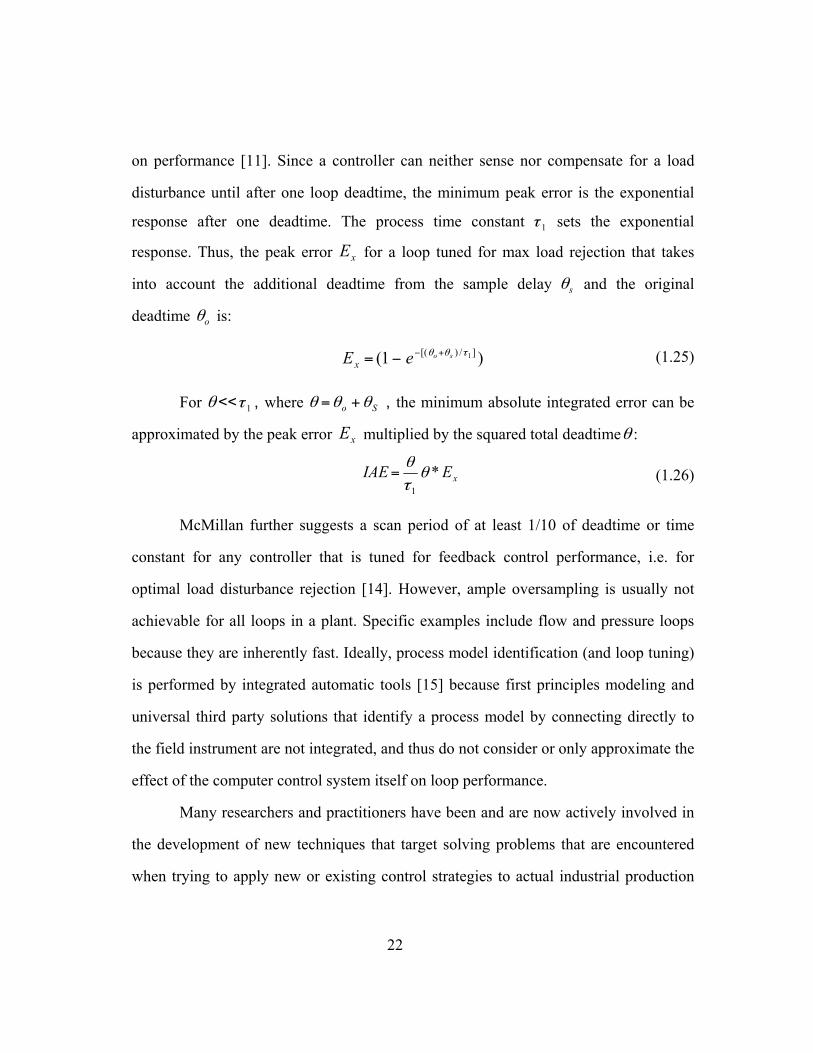
Figure 2.12: Effect of model mismatch in τ1 (2nd order process) ......................................45

Figure 2.13: Effect of move penalty R on the integral absolute error of different

controllers subject to an unmeasured disturbance of 1. Process: K=1; τ1

=30s; τ2=20s; Θ =1; MPC: P=30; M=9; Q=1; PID: KC=52.5; Ti=28;

Td=5.7 (Skogestad tuning) ............................................................................46

Figure 2.14: Effect of move penalty R in the presence of model mismatch on

processes of different order. Process: K=1, τ1 =30, τ2=20s, Θ =1; PID:

KC=52.5, Ti=28, Td=5.7 (Skogestad); MPC: P=30, M=9, Q=1 ....................47

xiv

Figure 2.15: Effect of Control Horizon to control performance with perfect model on

the integral absolute error of different controllers exposed to an

unmeasured disturbance of 1. Process: K=1; τ1 =30s; τ2=20s; Θ =1;

MPC: P=30; M=9; Q=1; PID: KC=52.5; Ti=28; Td=5.7 (Skogestad

tuning), DMC is off scale .............................................................................48

Figure 2.16: Effect of Control Horizon to control performance in the presence of

model mismatch on processes of different order. Process: K=1, τ1 =30,

τ2=20s, Θ =1; PID: KC=52.5, Ti=28, Td=5.7 (Skogestad); MPC: P=30,

M=9, Q=1 .....................................................................................................49

Figure 3.1: Schematic overview of optimization method: MPC tuning and design

parameters are calculated based on model parameters and model

mismatch .......................................................................................................53

Figure 3.2 Optimal tuning of model mismatch in process gain .........................................55

Figure 3.3 Optimal tuning of model mismatch in first order time constant ......................56

Figure 3.4 Optimal tuning of model mismatch in second order time constant ..................58

Figure 3.5: Optimal tuning map for model mismatch in K and τ1 of MPC with general

Kalman filter state update .............................................................................60

Figure 3.6: Optimal tuning map for model mismatch in K and τ1 of MPC with

simplified Kalman filter state update ............................................................62

Figure 3.7: Illustration of two-dimensional model mismatch subspace example with

Kactual=2±0.5 and Tactual=20s±5s ....................................................................64

Figure 3.8: Illustration of two-dimensional model mismatch example with

Kactual=2±0.5 and Tactual=20s±5s ....................................................................65

xv

Figure 3.9: Schematic overview of revised optimization method: MPC tuning and

design parameters are calculated based on model and model mismatch

range..............................................................................................................66

Figure 3.10: Schematic overview of revised method that includes MPC and observer

tuning and a modified MPC model-based on model and model mismatch

range..............................................................................................................68

Figure 4.1: Time Series of controlled variable (pressure) of loop with suboptimal and

optimal tuning, i.e. before and after lambda tuning; most of the variation

is due to process noise, not tuning ................................................................71

Figure 4.2: Autocorrelation of controlled variable (pressure) of loop with suboptimal

and optimal tuning, i.e. before and after lambda tuning; most of the

autocorrelation can be removed with tuning.................................................72

Figure 4.3: Application of optimal tuning method to MPC for manual tuning .................75

Figure 4.4: Application of optimal tuning method to MPC for adaptive tuning with

external property estimator (e.g. Neural Network) .......................................76

Figure 4.5: Adaptive control techniques ............................................................................77

Figure 4.6: Application of optimal tuning method to MPC for adaptive tuning with

state estimator (without need for property estimation) .................................79

Figure 4.7: P&ID of binary distillation column used for experimental testing of

proposed methods .........................................................................................82

Figure 4.8: Schematic diagram of OPC connection between MATLAB laptop and

DeltaV Control system. OPC is an open standard by the OPC foundation

[55] for open communication between windows based computers and

industrial plant automation. ..........................................................................84

xvi

Figure 4.9: Level control at steam rate of 0.55 kg/min for different MPC tuning,

ϭR=50=0.057, ϭR=100=0.066, ϭR=1000=0.052, ϭPID=0.036 .................................85

Figure 4.10: Level control after introduction of artificial unmeasured disturbance in

steam flow: steam flow loop setpoint was changed from 0.55kg/min to

0.4 kg/min; IAER=50=0.122, IAER=100=0.468, IAER=1000=∞ (control was

unsatisfactory and the plant had to stabilized with manual intervention),

IAEPID=0.3 ....................................................................................................85

Figure 4.11: Level control at steam rate of 0.4 kg/min for different MPC tuning,

ϭR=50=0.053, ϭR=100=0.028, controller with RMPC=1000 did not control

plant satisfactory and tripped accumulator pump interlock repeatedly,

ϭPI=0.032 .......................................................................................................87

Figure 4.12: Level control at steam rate of 0.4 kg/min for different MPC tuning,

ϭR=50=0.053, ϭR=100=0.028, controller with RMPC=1000 did not control

plant satisfactory and tripped accumulator pump interlock repeatedly,

ϭPI=0.032 .......................................................................................................88

Figure 4.13: Autocorrelation of prediction error in MPC at the three different tuning

settings at steam rate of 0.55 kg/min ............................................................90

Figure 4.14: Autocorrelation of prediction error in MPC at the three different tuning

settings at steam rate of 0.4 kg/min ..............................................................91

Figure 4.15: Autocorrelation of prediction error in MPC at the three different tuning

settings during rejection of unmeasured disturbance (steam rate changes

from 0.55kg/min to 0.4 kg/min)....................................................................91

xvii

Figure 4.16: Autocorrelation of level for MPC at the three different tuning settings at

steam rate of 0.55 kg/min, autocorrelation of level for well tuned PI

control is added for comparison – MPCR=1000 stands out significantly,

easy to determine tuning problems ...............................................................93

Figure 4.17: Autocorrelation of level for MPC at the three different tuning settings

during rejection of unmeasured disturbance (steam rate changes from

0.55kg/min to 0.4 kg/min), autocorrelation of level for well tuned PI

control is added for comparison – no controller stands out significantly,

this analysis for tuning problems may not be very conclusive .....................93

Figure 4.18: Application of optimal tuning method to MPC for adaptive tuning with

state estimator (without need for property estimation) .................................96

Figure 5.1: Screenshot of operator interface in chemical plant comparing PID and

MPC disturbance rejection performance ....................................................100

Figure 5.2: Disturbance rejection response K=1 T1=50 T2=0 θ=1, PID: (Skogestad)

Kc=25 Ti=8 Td=0, MPC: P=10 M=3 Q=1; on left a) R=0.1, on right b)

R=0.01 ........................................................................................................106

Figure 5.3: Feedback control performance depending on model mismatch and penalty

tuning, K=1 T1=50 T2=0 θ=1, PID: (Skogestad) Kc=25 Ti=8 Td=0, MPC:

P=10 M=3 Q=1; on left a) R=0.1, on right b) R=0.01 ................................107

Figure 5.4: Step response of 20 interacting lags [8] ........................................................109

Figure 5.5: Feedback control performance depending on model mismatch and penalty

tuning, K=1 T1=50 T2=0 θ=1, PID: (Skogestad) Kc=25 Ti=8 Td=0, MPC:

P=10 M=3 Q=1; on left a) R=0.1, on right b) R=0.01 ................................110

xviii

Figure 5.6: Oscillation due to model mismatch (τ/τ =2) on first order (left - a) and

second order (right - b) processes, 150 1 and 1 30 1 20 1 . PID: (Skogestad) Kc=25 Ti=8

Td=0, MPC: Q=1 R=0.01; on left a) FOPDT, P=10 M=3 on right b)

SOPDT P=30 M=9 .....................................................................................111

Figure 5.7: Unit step disturbance of PI controllers with different tuning settings.

(FOPDT model: K=1, θ=4, τ=20). Ref [72] ...............................................114

Figure 5.8: Tunable integral action in the feedback path of a model predictive

controller .....................................................................................................115

Figure 5.9: Comparison of load rejection performance before and after adding tunable

integral action to the future error vector calculation...................................117

Figure 5.10: Comparison of robustness before and after adding tunable integral action

to the future error vector. ............................................................................118

Figure 5.11: Comparison of robustness and performance with manual tuning of

integral action on the future error vector ....................................................118

Figure 5.12: Comparison of robustness and performance with manual tuning of

integral action on the future error vector on second order process .............119

1

Chapter 1

Introduction

Process control is a major consideration of almost all installations of chemical,

pharmaceutical and refining industries, and a multibillion-dollar business worldwide.

Although the best possible control has not always been a major focus in industry over

the past 50 years, in recent years new plants are increasingly designed with

controllability and optimizability in mind. Additionally, many existing plants are being

renovated with this objective as well. Optimization in this sense includes geometry of

the installed hardware, such as reactors, tanks, pipes location, etc., but also the locations

of control elements and measurements. With the increasing cost of natural resources

and the effective costs associated with undesirable emissions, energy consumption has

also become a great factor in plant design. Control performance monitoring in

combination with controller retuning or model scheduling can dramatically improve the

efficiency of industrial plants, thereby saving millions of dollars annually. Another

technique that has become increasingly popular among industrial plants in recent years

is abnormal situation monitoring and prevention. Modern device and control system

include novel sensor designs and embedded statistical algorithms that are able to

predict potential failures or upcoming maintenance cycles. Common measurement

device and actuator failures include plugged lines, heat transfer change due to fouling,

and control element failures or nonlinearities due to build-up in valves or failures in

positioners. Predictive maintenance systems can dramatically increase the uptime of

plant operations and prevent costly and dangerous manifestations of unexpected

2

shutdowns. The reliability of these techniques has significantly increased in the last

decade.

1.1 Process model mismatch in industrial processes

In the United States and Canada, process control systems are usually

commissioned by a local business partner of the control system vendor. However, some

end users have enough in-house capacity to commission and maintain a complete

control system themselves. In Europe and Asia, often a local subsidiary representing

the control system vendor is employed for that task. In either case, the commissioning

costs of a control system are substantial, and it is rarely practical to pay detailed

attention to every control loop configuration in a plant. About 90% of all loops are

controlled by traditional linear controllers such as PID. Most instances of advanced

control strategies are also linear, such as model predictive control (MPC). While linear

controllers are predominantly used, the majority of real processes exhibit nonlinear

behavior. The obvious consequence of this discrepancy is that model mismatch is

unavoidable. Unaddressed model mismatch not only results in suboptimal control

performance, but also nullifies many of the advantages of the aforementioned

technologies that may have otherwise improved control performance and uptime.

Therefore, model mismatch is not only costly, but also diminishes cost savings of other

technologies. This is the main motivation for this research.

Practical ways to address model mismatch resulting from nonlinearity include

linearization of control elements and transmitters, and controller gain scheduling.

Simple linearization functions are built into most automation systems and intelligent

field devices. One practical method that is frequently used for addressing model

3

mismatch from nonlinearity and plant drift is tuning a controller for the worst case

scenario (e.g., highest process gain) and accepting suboptimal tuning for other regions

of the process. The default tuning parameters of an industrial PID controller are

conservative in order to work, at least initially, for a variety of processes applications.

Unfortunately, one finds that frequently controller tuning parameters are left at their

default values indefinitely.

Model mismatch that results from identification error or from plant drift is more

difficult to address—it is hard to detect because sufficient process perturbation is

required, which contradicts the objective of control. Furthermore, it is hard to

distinguish from unmeasured disturbances. Chapter 2 will go on to discuss previous

research in this area.

1.2 Model Predictive Control

Linear model predictive control refers to a class of control algorithms that

compute a manipulated variable profile by utilizing a linear process model to optimize a

linear or quadratic open-loop performance objective subject to linear constraints over a

future time horizon. The first move of this open loop optimal manipulated variable

profile is then implemented. This procedure is repeated at each control interval, and the

process measurements are used to update the optimization problem as shown in Figure

1.1.

Figper

mo

con

mo

tech

pro

the

pro

the

and

gure 1.1: receriod, only the

This cla

ving horizon

ntrol. The co

del. These m

hniques that

ocesses can e

open-loop

ogramming a

Shown

state-space

d x is the vec

eding horizoe first one u0

ass of contro

n control—h

ontroller use

models can

t do not requ

easily be han

performanc

algorithms.

below is the

formulation

ctor of states

on control: m0 is impleme

ol algorithms

has several

s a linear tra

be obtained

uire a signifi

ndled by sup

ce objective

e discrete dy

n, in which y

s.

1ˆk kx Ax+ =

4

m control moented

s—also refer

advantages

ansfer functi

d from proc

icant fundam

perposition o

e is perform

ynamical sys

y is the vecto

k kBu+ k =

ˆ ˆk ky Cx=

oves are calcu

rred to as rec

for applicat

ion, state sp

cess tests us

mental mode

of the linear

med by eit

stem model

or of outputs,

0,1,2,...

ulated at eve

ceding horiz

tion in chem

ace, or conv

sing time se

eling effort. M

models. Op

ther linear

used by the

, u is the vec

ery execution

zon control o

mical proces

volution plan

eries analysi

Multivariabl

ptimization o

or quadrati

e controller i

ctor of input

(1.1

(1.2

n

or

ss

nt

is

le

of

ic

is

s,

1)

2)

5

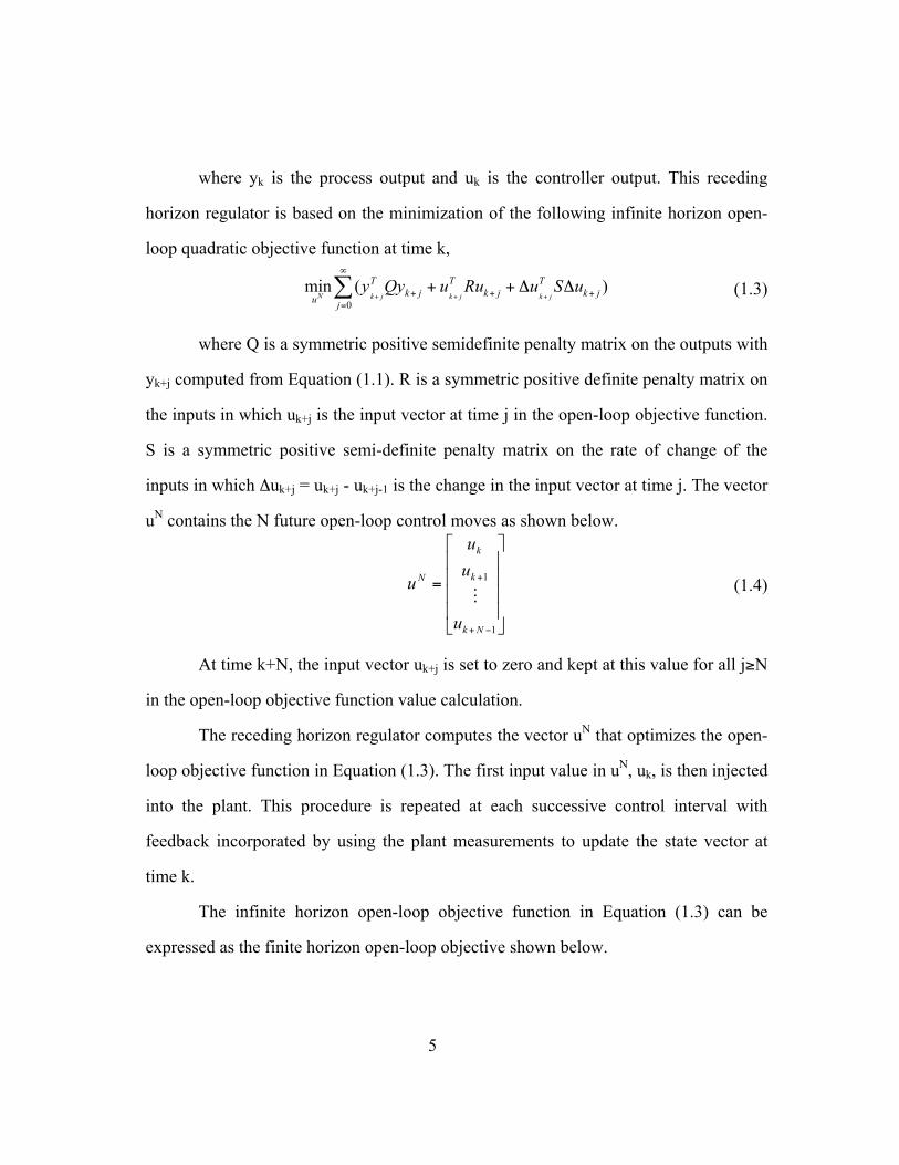
where yk is the process output and uk is the controller output. This receding

horizon regulator is based on the minimization of the following infinite horizon open-

loop quadratic objective function at time k,

0

min ( )N k j k j k j

T T Tk j k j k ju j

y Qy u Ru u S u+ + +

∞

+ + +=

+ + Δ Δ∑

(1.3)

where Q is a symmetric positive semidefinite penalty matrix on the outputs with

yk+j computed from Equation (1.1). R is a symmetric positive definite penalty matrix on

the inputs in which uk+j is the input vector at time j in the open-loop objective function.

S is a symmetric positive semi-definite penalty matrix on the rate of change of the

inputs in which Δuk+j = uk+j - uk+j-1 is the change in the input vector at time j. The vector

uN contains the N future open-loop control moves as shown below.

⎥⎥⎥⎥

⎦

⎤

⎢⎢⎢⎢

⎣

⎡

=

−+

+

1

1

Nk

k

k

N

u

uu

uM

(1.4)

At time k+N, the input vector uk+j is set to zero and kept at this value for all j≥N

in the open-loop objective function value calculation.

The receding horizon regulator computes the vector uN that optimizes the open-

loop objective function in Equation (1.3). The first input value in uN, uk, is then injected

into the plant. This procedure is repeated at each successive control interval with

feedback incorporated by using the plant measurements to update the state vector at

time k.

The infinite horizon open-loop objective function in Equation (1.3) can be

expressed as the finite horizon open-loop objective shown below.

6

)(minmin1

0jk

Tjkjk

Tjk

N

juNkTNkNk

TNk

uk uSuQyyuSuyQy

NN++++

−

=++++ ΔΔ++ΔΔ+=Φ ∑ (1.5)

The output penalty term in Equation (1.3) has been replaced with the

corresponding state penalty term in Equation (1.5). Determination of the terminal state

penalty matrix, Q , depends on the stability of the plant model.

For stable systems, Q in Equation (1.5) is defined as the infinite sum in

Equation (1.6).

)(0∑∞

=

=i

iTT QCACAQi

(1.6)

This infinite sum can be determined from the solution of the following discrete

Lyapunov equation:

AQAQCCQ TT += (1.7)

There are standard methods available for the solution of this equation.

Straightforward algebraic manipulation of the quadratic objective presented in Equation

4 results in the following quadratic program for uN:

)()(2)(min 1−−+=Φ kkTNNTN

uk FuGxuHuu

N (1.8)

The matrices H, G, and F are computed as shown below with determined from

Equation (1.7).

⎥⎥⎥⎥⎥

⎦

⎤

⎢⎢⎢⎢⎢

⎣

⎡

++

++−

−++

=

−−

−

−

SRBQBBAQBBAQB

BQABSRBQBSABQBBQABSBQABSRBQB

H

TNTNT

NTTTT

NTTTTT

2

22

21

2

1

K

MOMM

K

K

7

⎥⎥⎥⎥⎥

⎦

⎤

⎢⎢⎢⎢⎢

⎣

⎡

=

NT

T

T

AQB

AQBAQB

GM

2

,

⎥⎥⎥⎥

⎦

⎤

⎢⎢⎢⎢

⎣

⎡

=

0

0M

S

F

The discussion of instable systems begins with partitioning the Jordan form of

the A matrix into stable and unstable parts in which the unstable eigenvalues of A are

contained in Ju.

[ ] ⎥⎦

⎤⎢⎣

⎡⎥⎦

⎤⎢⎣

⎡== −

s

u

s

usu V

VJ

JVVVJVA ~

~

001 (1.9)

The stable and unstable modes, zs and zu respectively, then satisfy the following

relationships:

xVV

zz

s

us

u

⎥⎦

⎤⎢⎣

⎡=⎥

⎦

⎤⎢⎣

⎡~~

(1.10)

k

s

usk

uk

s

usk

uk Bu

VV

zz

JJ

zz

⎥⎦

⎤⎢⎣

⎡+⎥

⎦

⎤⎢⎣

⎡⎥⎦

⎤⎢⎣

⎡=⎥

⎦

⎤⎢⎣

⎡

+

+~~

00

1

1

(1.11)

For unstable plants, the finite horizon open-loop objective function in Eq. 4 is

subject to the following equality constraint on the unstable modes at time k+N.

0~== ++ Nku

uNk xVz (1.12)

This equality constraint is required if the unstable modes are not brought to zero

at time k+N, they evolve uncontrolled after this time and do not converge to zero.

Therefore, the optimal solution to (1.5) must be a vector uN that zeroes the unstable

modes at time k+N.

8

With the equality constraint ensuring that only the stable modes contribute to

the value of kΦ after time k+N-1, Q for unstable systems can be computed from the

stable modes in a manner similar to Equation (1.6).

Muske and Rawlings (1992) show that this regulator formulation guarantees

nominal stability for all choices of tuning parameters satisfying the conditions outlined

in the previous sections. Nominal stability comes from the evaluation of the state

penalty on an infinite horizon even though there are a finite number of decision

variables. Previous model predictive controller formulations are finite horizon. The

absence of nominal stability in these implementations is a direct consequence of the

finite horizon formulation of the control algorithm. Bitmead et al. (1990) demonstrate

that nominal stability cannot be guaranteed for a finite receding horizon regulator.

Kwon and Pearson (1978) propose a nominally stabilizing receding horizon

regulator based on a finite horizon objective subject to a terminal state constraint. The

terminal constraint forces all of the modes of the system to be zero at the end of the

horizon instead of only the unstable modes. This constraint leads to aggressive control

action with small values of N for both stable and unstable systems since the regulator

approaches a deadbeat controller. Feasibility of this terminal constraint also requires

that the system be completely controllable. Additionally, Rawlings and Muske’s proof

requires the systems to be stabilizable and uncontrollable modes to reach origin in

infinite steps.

Industrial implementations began with model algorithmic control (MAC)

developed by Richalet et al. (1978) and dynamic matrix control (DMC) developed by

Cutler and Ramaker (1980). These Shell Oil engineers developed their own

independent MPC technology in the early 1970's, with an initial application in 1973.

9

Cutler and Ramaker presented details of an unconstrained multivariable control

algorithm which they named Dynamic Matrix Control (DMC) at the 1979 National

AIChE meeting and at the 1980 Joint Automatic Control Conference. In a companion

paper at the 1980 meeting, Prett and Gillette described an application of DMC

technology to an FCCU reactor/regenerator. DMC technology uses linear step response

or impulse response models of the process. The optimal control path is pre-calculated

off-line and stored in a large matrix. This controller matrix is then used to compute the

on-line moves of the manipulated variables by superposition. As a result, computational

cost is reduced drastically in comparison to MPC methods that solve the above optimal

equations on-line. Another advantage of DMC technology is that the state variable is

calculated intuitively from the model, and represents the explicit future output

prediction. This means that the future prediction of process outputs such as constraints

is readily available and can be displayed to the user.

Other early technology implementation include IDCOM (1978) by Richalet et

al. and linear dynamic matrix control (LDMC), which uses a linear objective function

and incorporates constraints explicitly, by Morshedi et al. (1985). Garcia and Morshedi

(1986) discuss quadratic dynamic matrix control (QDMC), which is an extension of

DMC incorporating a quadratic performance function and explicit in corporation of

constraints. Grosdidier et al. (1988) present IDCOM-M, which is an extension of

IDCOM using a quadratic programming algorithm to replace the iterative solution

technique of the original implementation. Marquis and Broustail (1988) discuss Shell

multivariable optimizing control (SMOC), which is a state-space implementation.

10

1.3 Control performance criteria

The performance of industrial controllers can be measured in various ways. A

comprehensive overview of control performance assessment technologies is given in

[6]. Different processes may have greatly different quality and safety requirements;

thus, plant engineers may use one or multiple performance criteria, such as overshoot,

arrest time (time to reach setpoint for integrating processes), oscillation characteristics,

integrated error, and integrated absolute error for their evaluation of loop performance.

Furthermore, the measured control performance for a given controller may be a tradeoff

between setpoint tracking and disturbance rejection behavior. Traditional PID control,

which still is the most popular controller choice in the process industries, suffers from

this problem. Many practical approaches such as structure modifications or setpoint

filtering have been developed to address this problem. Also, modern model predictive

control algorithms have been specifically reformulated to eliminate this disadvantage.

An example by Badgwell and Muske is described in [20]. Additionally, section 1.4

further discusses tuning techniques for specific control objectives. Finally, a general

overview of commercially available MPC algorithms is given by Qin and Badgwell

[32].

Shinskey [8] suggests a performance criteria that is a normalized value of the

integrated error defined as:

q d

IEqK τΔ

(1.13)

where Δq is the unmeasured disturbance, Kq is the process gain, τd is the

deadtime and IE is the integrated error calculated by:

(1.14)

11

where y(t) is the controlled process output variable and SP(t) is the operator

setpoint. Since fractional deadtime is a very important factor for control performance,

Shinskey shows why controllers that consider deadtime in their equations, such as

model-based, direct synthesis and PIDτd [8] generally have better control performance

in the deadtime dominant region. However, he also shows that in the other regions the

control performance of model-based controllers is generally suboptimal, i.e. the

normalized integrated error is equal to one throughout [8], which can be seen in Figure

1.2 (internal model control is indicated as IMC). The dashed curve labeled “best”

describes the minimum IE attainable for any feedback controller. All controllers are

tuned to minimize the integrated absolute error (IAE) in the controlled variable

following a step change in the load introduced at the controller output. The IE

represented by the flat line at 1.0 on the normalized scale is produced by an unfiltered

internal model controller (IMC). This controller shows the lowest performance of all

controllers for lag-dominant processes. Additional filtering only increases IE, in direct

ratio of the filter time to the deadtime proportion in the loop. A Smith predictor and any

other model-predictive controller whose parameters are simply matched to the process

parameters show the same performance as IMC.

12

Figure 1.2: Control performance dependence on fractional deadtime for different controllers, Source: F. G. Shinskey [8]

This research does not explore performance improvements for deadtime-

dominant processes, because it is generally known that model predictive control is

already superior in that region of fractional deadtime. Instead, the research is seeking to

improve the control performance in the lag-dominant and intermediate regions.

Furthermore, since some tuning settings (that will be discussed in the following

sections) can lead to oscillatory behavior around the setpoint, thereby creating negative

error, this research uses the normalized value of the absolute value of the integral error

(IAE) for all comparisons and diagrams:

q d

IAEqK τΔ

(1.15)

where Δq is the unmeasured disturbance, Kq is the process gain, τd is the

deadtime and IAE is the integrated absolute error calculated by:

13

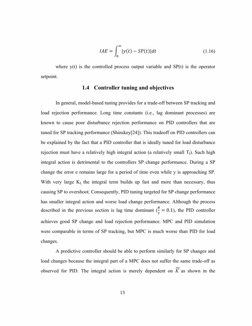
| | (1.16)

where y(t) is the controlled process output variable and SP(t) is the operator

setpoint.

1.4 Controller tuning and objectives

In general, model-based tuning provides for a trade-off between SP tracking and

load rejection performance. Long time constants (i.e., lag dominant processes) are

known to cause poor disturbance rejection performance on PID controllers that are

tuned for SP tracking performance (Shinskey[24]). This tradeoff on PID controllers can

be explained by the fact that a PID controller that is ideally tuned for load disturbance

rejection must have a relatively high integral action (a relatively small TI). Such high

integral action is detrimental to the controllers SP change performance. During a SP

change the error e remains large for a period of time even while y is approaching SP.

With very large KI, the integral term builds up fast and more than necessary, thus

causing SP to overshoot. Consequently, PID tuning targeted for SP change performance

has smaller integral action and worse load change performance. Although the process

described in the previous section is lag time dominant ( 0.1), the PID controller

achieves good SP change and load rejection performance. MPC and PID simulation

were comparable in terms of SP tracking, but MPC is much worse than PID for load

changes.

A predictive controller should be able to perform similarly for SP changes and

load changes because the integral part of a MPC does not suffer the same trade-off as

observed for PID. The integral action is merely dependent on K as shown in the

14

previous section. Also, the error e does not increase while y is approaching SP in a

predictive controller. Theoretically, it can be zero after the first execution cycle. This is

only true when assuming that the prediction (state) is updated effectively and doesn’t

add additional significant time constants. But the fact that the MPC load disturbance

performance is slower during the simulation indicates that the state is updated too

slowly (i.e., without consideration of the error derivative). In the absence of model

mismatch, state update only comes into play during load changes, not during SP

changes. Therefore, this simulation is a good preliminary test for the research.

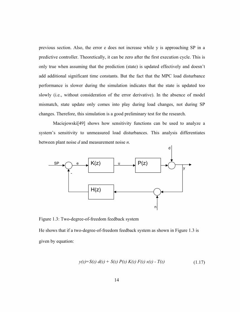
Maciejowski[49] shows how sensitivity functions can be used to analyze a

system’s sensitivity to unmeasured load disturbances. This analysis differentiates

between plant noise d and measurement noise n.

Figure 1.3: Two-degree-of-freedom feedback system

He shows that if a two-degree-of-freedom feedback system as shown in Figure 1.3 is

given by equation:

y(z)=S(z) d(z) + S(z) P(z) K(z) F(z) s(z) - T(z) (1.17)

P(z) K(z)

-

H(z)

SP u

d

y e

n

15

the sensitivity function S(z) is:

S(z) = [I + P(z) K(z) H(z)]-1 (1.18)

and the complementary sensitivity function T(z) is:

T(z) = [I + P(z) K(z) H(z)]-1 - P(z) K(z) H(z) (1.19)

Systems with ‘smaller’ sensitivity functions must have better feedback control

action. Unfortunately, it is not possible to design a two-degrees of freedom controller

that has very low sensitivity and very low complementary sensitivity because these

traits are determined by each other:

S(z) + T(z) = I (1.20)

Since S(z) and T(z) are complex however it is possible to for them to be large at

the same time, i.e., it is possible to design a very bad feedback controller.

From the above equations it can be seen that the setpoint change response can

be designed independently from the load-rejection response. However, these two

responses will be significantly different, the setpoint response transfer function is

S(z)P(z)K(z), while the load rejection transfer function is S(z). This fact also supports

the findings of the previous section.

The ideal continuous time domain PID controller is expressed in the Laplace

domain as follows:

( ) ( ) ( )cU s G s E s= (1.21)

16

where

1( ) (1 )c c di

G s K T sT s

= + + (1.22)

and where Kc is the proportional Gain, Ti is the integral time constant and Td is

the derivative time constant. Tuning PID controllers always presents the challenge of

correctly specifying the tradeoff setpoint tracking vs. disturbance rejection

performance. A specific textbook tuning method will favor either setpoint tracking or

disturbance rejection. Many model-based tuning rules match the internal parameters of

PID to internal parameters of a model for the process to be controlled. Methods such as

pole cancelation and lambda tuning match the integral time of the controller to the

dominant time constant of the process. The controller gain K is set to achieve a certain

closed-loop time constant and a certain setpoint change response (e.g., no overshoot).

Since the resulting integral action of such controllers is relatively small, it exhibits very

good setpoint change performance, but poor disturbance rejection performance.

Empirical PID tuning methods, such as Ziegler-Nichols, are specifically designed for

disturbance rejection performance. The integral action of such controllers is strong

enough to return the process variable to the setpoint very quickly, but leads to undesired

setpoint overshoot. Figure 1.4 compares the load change and setpoint change responses

of two PID controllers. Both control the same process with the following transfer

function: . The tuning for the first PID controller is obtained by using

IMC tuning rules 1 2IMCiθ

τ τ= + resulting in KC=20.2, Ti=50.5s, Td=0.49505s, which

favors setpoint tracking performance. The tuning for the second PID controller is obtained by using Skogestad’s tuning rules [9] 28

Skogestadiτ θ τ= + resulting in KC=25,

Ti=8s, Td=0s, which is significantly different and favors load disturbance rejection

17

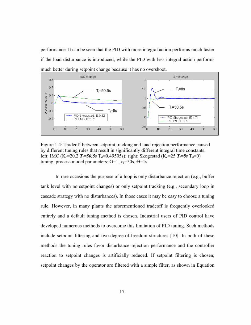
performance. It can be seen that the PID with more integral action performs much faster

if the load disturbance is introduced, while the PID with less integral action performs

much better during setpoint change because it has no overshoot.

Figure 1.4: Tradeoff between setpoint tracking and load rejection performance caused by different tuning rules that result in significantly different integral time constants. left: IMC (Kc=20.2 Ti=50.5s Td=0.49505s); right: Skogestad (Kc=25 Ti=8s Td=0) tuning, process model parameters: G=1, τ1=50s, Ө=1s

In rare occasions the purpose of a loop is only disturbance rejection (e.g., buffer

tank level with no setpoint changes) or only setpoint tracking (e.g., secondary loop in

cascade strategy with no disturbances). In those cases it may be easy to choose a tuning

rule. However, in many plants the aforementioned tradeoff is frequently overlooked

entirely and a default tuning method is chosen. Industrial users of PID control have

developed numerous methods to overcome this limitation of PID tuning. Such methods

include setpoint filtering and two-degree-of-freedom structures [10]. In both of these

methods the tuning rules favor disturbance rejection performance and the controller

reaction to setpoint changes is artificially reduced. If setpoint filtering is chosen,

setpoint changes by the operator are filtered with a simple filter, as shown in Equation

Ti=50.5s

Ti=8s Ti=50.5s

Ti=8s

18

(1.24). This effectively flattens the step change of the operator and creates a smaller

slope as setpoint, thereby preventing overshoot.

(1.23)

Where SP is the operator and SP* is the working setpoint. Equation (1.24)

shows a two-degree-of-freedom approach that factors the controller gain out,

effectively separating the setpoint and disturbance behavior [10]. The setpoint

weighting factor is bounded, 0 1, and becomes a new tuning parameter for the

controller.

[ ]0

1( ) ( ) ( ) ( )t

mc c D

I

dyp t p K SP t y t K e t dtdt

β ττ⎡ ⎤

= + − + −⎢ ⎥⎣ ⎦∫ (1.24)

In the case of lambda tuning for integrating processes, overshoot can be

prevented by setting the filter factor equal to lambda [7]. PID algorithms are often

referred to as two-degree-of-freedom (also known as 2DOF) if the calculation of

derivative action is factored out of the PID equation and only applied to the process

variable (instead of applying it to the error which reflects setpoint changes). Shinskey

proposed a modification [8] which eliminates the performance tradeoff and improves

performance for deadtime-dominant processes (See also Figure 1.2). In general,

different tuning methods have to be chosen for different control objectives. The

performance tradeoff described above is one of the reasons why so many tuning

methods have been proposed for PID tuning, along with the fact that tuning rules use

different input variables. While the tuning examples shown in Figure 1.4 calculate

tuning parameters based on a process model, other methods calculate it based on other

process characteristics. For example, Ziegler-Nichols rules ask for critical gain and

19

critical frequency, which may be easy to determine for some mechanical processes but

not practical for many industrial chemical processes. Aström and Hӓgglund developed

a relay oscillation method that can bring a system into sustained self-oscillation at

controllable amplitude, resulting in equally useful oscillations that are much less

intrusive to the process [42]. In combination with original or modified Ziegler-Nichols

tuning rules, this technique is used in many commercial products, such as the digital

automation system DeltaV [43]. O’Dwyer summarizes about 300 different tuning

methods in his research [19].

Model predictive controllers generally do not have a performance tradeoff

between setpoint tracking and disturbance rejection because the terms for error and

move penalty are inherently separate.

1ˆk k kx Ax Bu+ = + 0,1,2,...k = (1.1)

ˆ ˆk ky Cx= (1.2)

0

min ( )N k j k j k j

T T Tk j k j k ju j

y Qy u Ru u S u+ + +

∞

+ + +=

+ + Δ Δ∑

(1.3)

where Q, R, S are the penalty weights for error, controller move and

incremental move, xk is the model state matrix, yk is the process output and uk is the

controller output.

However, they still need to be tuned for a specific multivariable process control

objective. While the process model is always matched with the internal structure of an

MPC controller (e.g., state space with state space MPC formulation), additional tuning

parameters determine the behavior with respect to setpoint change and disturbance

rejection. The penalty vectors can be used to emphasize one variable over others in

20

accordance with the control objective for the specific process as defined by the end

user. If model mismatch is suspected, Q and R can also be used to make the controller

more robust (i.e., detuning). However, methods such as funnel control or reference

trajectory have a more obvious impact on robustness as they effectively filter the error

vector—which is why they are the preferred means for engineers and operators to tune

model predictive controllers in industrial process applications. Since a model predictive

controller inherently “matches” the process, the control moves are always optimal for

the specific process model. This means that the controller can only be detuned

(according to physical limitations on the final control elements) and never tuned very

aggressively. For example, a valve opening speed can never be infinite; therefore, the

value of R can never realistically be zero. It is known and discussed by many authors

(e.g., Shinskey [24]) that the disturbance rejection of industrial MPC controllers lags

behind that of PID controllers when they are specifically tuned for disturbance

rejection. Recent MPC improvements in the area of state update [20] have closed that

performance gap if the observer model is assumed to be known perfectly. However, in

the presence of model mismatch, the control performance (IAE) of a PID controller is

still better than that of an MPC controller with the best possible tuning (see Figure

2.10).

Lundstrom, Lee, Morari and Skogestad [21] discuss limitations of dynamic

matrix control (DMC), such as suboptimal feedback performance for input disturbances

and problems with instable processes. Their paper shows how MPC with an observer

can be used to improve the feedback control performance. Some of the limitations

discussed by Lundstrom, et al will become apparent in following chapters. When DMC

is compared to MPC with observers, usually a large performance gap can be observed

21

(see Figure 2.11). Though observers improve MPC feedback performance, they still

have assumptions that empirically tuned controllers, such as PID, do not have. Any

model-based predictive controller and model-based observer will assume that the model

is known perfectly. Even small model errors can cause large prediction and state update

errors. Various correction or filter methods are utilized to reduce the impact of model

error, but obviously optimality cannot be guaranteed if model error occurs. Even

though many industrial processes are minimum phase, the majority of closed loops are

not. Time delay, also known as deadtime, and higher-order lags create right hand poles

that greatly complicate tuning. In most instances, closed-loop deadtime is created by

transport delay of material in pipes and discrete sampling mechanisms that are

unavoidable in computer control systems, while higher order lags are usually a result of

filter time constants in measuring and control devices.

Other challenges often found in industrial plants are resolution and deadband

problems created by the mechanical behavior of valves and packing. Mechanical

limitations lead to stick-slip behavior, which causes non-linearities for small moves in

manipulated variable. These limitations present many challenges to control engineers in

industrial plants. Even if a certain process is expected to act like a first-order filter with

certain gain and time constant depending on vessel geometry, one has to consider

additional time constants from transmitters, control elements computer sampling, and

jitter. Usually one should not rely solely on first principles models that may be

available for some of the reactions. Since any digital control system has CPU and

communication constraints, ample oversampling is not practical for all types of loops in

a plant. A sampling rate of 1/5 of the dominant time constant is often considered

reasonably sufficient. McMillan et al. discuss the impact of deadtime and sample period

22

on performance [11]. Since a controller can neither sense nor compensate for a load

disturbance until after one loop deadtime, the minimum peak error is the exponential

response after one deadtime. The process time constant 1τ sets the exponential

response. Thus, the peak error xE for a loop tuned for max load rejection that takes

into account the additional deadtime from the sample delay sθ and the original

deadtime oθ is:

)1( ]/)[( 1τθθ soeEx+−−= (1.25)

For θ<< 1τ , where So θθθ += , the minimum absolute integrated error can be

approximated by the peak error xE multiplied by the squared total deadtimeθ :

xEIAE *1

θτθ

= (1.26)

McMillan further suggests a scan period of at least 1/10 of deadtime or time

constant for any controller that is tuned for feedback control performance, i.e. for

optimal load disturbance rejection [14]. However, ample oversampling is usually not

achievable for all loops in a plant. Specific examples include flow and pressure loops

because they are inherently fast. Ideally, process model identification (and loop tuning)

is performed by integrated automatic tools [15] because first principles modeling and

universal third party solutions that identify a process model by connecting directly to

the field instrument are not integrated, and thus do not consider or only approximate the

effect of the computer control system itself on loop performance.

Many researchers and practitioners have been and are now actively involved in

the development of new techniques that target solving problems that are encountered

when trying to apply new or existing control strategies to actual industrial production

23

plants. Control conferences have been well-attended for decades, and there is an

abundance of new control papers and methods every year. The constant development

and improvement of modeling and control strategies makes the popularity of PID, a

more than 100 year-old control strategy, even more remarkable. Only few control

strategies that are alternatives to PID have actually found traction. Many MPC and

fuzzy logic based PID replacement controllers have fallen out of fashion.

The following innovations were targeted at solving some of the issues described

above. Addressing a great MPC weakness in 2002, Badgwell & Muske developed a

method to augment disturbances to the model matrix, thereby better accounting for

unmeasured dynamic disturbances in the feedback path [20]. This approach assumes

that the perfect process model is known. In 2001, Shinskey improved the deadtime

handling of PID control as he recognized this as a significant weakness in single loop

control[25]. His method makes PID control applicable to deadtime-dominant processes,

while simultaneously retaining very good feedback performance. However, it also

sacrifices robustness, one of the great benefits of PID control. An example of a new

PID replacement controller is Pannocchia, Laachi, and Rawlings’ “Candidate to

Replace PID Control - Constraint LQ”[41], developed in 2003, which exhibits very

good setpoint tracking performance. This algorithm is tailored for minimum IE if input

constraints reached; however, it also assumes the presence of a perfect model.

The research presented in this dissertation introduces two novel approaches for

improving MPC control performance. Chapter 3 discusses a new automated calculation

method for optimal tuning that is based on model mismatch, and Chapter 4 describes

how the method described in Chapter 3 can be used for closed loop adaptive control.

Chapter 5 introduces structural modifications to the MPC equation that improve the

24

disturbance rejection performance in the presence of model mismatch. Some of the PID

properties that are most likely responsible for its unmatched popularity will be utilized

to improve the MPC algorithm.

25

Chapter 2

State update methods and tuning

Model predictive controllers, like any model-based controller, are designed to

solve feed-forward specific control challenges, such as difficult process dynamics and

loop interaction. Therefore, it does not seem surprising that controllers designed only

for feedback control, such as PID, can perform better on processes that require

feedback correction. Feedback control is required whenever the controlled processes is

affected by unmeasured disturbances, has model mismatch, or exhibits nonlinear

behavior. Mismatch between model-based controller tuning and the actual process can

be encountered due to identification error or process drift. All of the listed conditions

exist in industrial processes. Thus, practical controllers have some method of

accounting for these conditions (i.e., feedback).

In a model predictive controller, the state update (or state correction) algorithm

is the mechanism that realizes control feedback as described below. The term “state

feedback” is used to describe the process of updating the state variable based on

process inputs and outputs. It is important to note the difference between state feedback

and control feedback described above. An “optimal state update,” as discussed in many

previous research papers, does not necessarily translate into optimal feedback control

performance. Control performance largely depends on the dynamics of the control

error. Figure 2.1 depicts the schematic diagram of a predictive controller with

embedded state observer:

26

C

process

J

B

controller

(Prediction)

kk yy ˆ−

kykekSP

kykx

uMVk ≅

Unmeasured disturbances

1 2 3

-

-

A

C’

Figure 2.1: predictive controller with integrated observer; dotted line indicates feedback path; A, B and C are constant matrices that are used to represent the process model; J is the observer gain matrix

Based on the error ke , the controller computes the optimal future outputs of

manipulated variables kMV over the control horizon. Ideally, the error vector is

calculated directly as the difference between future prediction vector x and setpoint

(SP) trajectory. However, the direct utilization of state variables is only possible in

controllers that are realized in terms of step response process (SR) models. According

to Qin and Badgwell[32], dynamic matrix control (DMC)[1] is the most commonly

used controller of that kind. In the case of minimum realization model-based control,

such as state space (SS), the future output prediction vector is not readily available and

has to be re-computed at every scan from the model (dashed line and C' in Figure 2.1).

27

Oftentimes an observer (Kalman filter) is used to correct the state variables for

conditions such as the disturbances as described above. Figure 2.1 shows the

implementation of this observer with Kalman filter gain, which is pre-calculated based

on what is known about the model before the controller is commissioned, i.e., it is a

constant during normal operation as will be discussed in the following sections of this

chapter. Assuming a constant gain matrix for J, it becomes apparent from Figure 2.1

that the feedback path between measurement and model-based controller introduces no

dynamic control elements and acts as a proportional only controller (P-controller). Even

though the calculation of the optimal J is mathematically refined, a P-only state

feedback may not necessarily translate into optimal feedback control performance.

State of the art state estimation theory can provide offset-free control for

positional MPC (e.g. Pannocchia and Kerrigan[44]). With incremental MPC controllers

such as dynamic matrix control, offset-free control is inherent because the incremental

controller equation:

eKdMV ⊗= (2.1)

acts as an integrator with

0

0

MVdteKMVpt

t

+⊗= ∫+

(2.2)

where K is the MPC controller gain matrix and e is the error vector calculated

from future prediction and the setpoint (SP) trajectory. The integration of the error

vector e occurs at every scan over the entire prediction horizon p. This shows that the

closed-loop control path as indicated by dotted line in Figure 2.1 can thus be considered

28

to incorporate a PI controller. However, this dynamic matrix based PI-controller is still

different from the traditional PI-controller described by

⎥⎥⎦

⎤

⎢⎢⎣

⎡+= ∫

t

tIP dteeKteKtu

0

)()()( (2.3)

because here an error scalar is integrated. In the settled case (no transients) the

I-term of a PID may be a nonzero constant, while the I-term of an MPC is zero at the

unconstrained steady state.

This chapter discusses the importance of state update in predictive controllers

and the optimal tuning of state update. Optimal state update in a model predictive

controller does not necessarily lead to optimal control performance, which will be

shown in the following chapters.

2.1 Modeling Techniques

State space (SS) models have become popular in the recent years. One of the

many advantages of SS models is that they allow minimum realization of models,

which reduces dimensionality of the model matrix when the process deadtime is

relatively small compared to the process time constants. This translates to a reduction

of states in state variable x . However, step response (SR) models are still preferred by

many users because they are more intuitive and can construct the future prediction

vector in a natural way. Commercial products usually display the future prediction to

operators and/or use it to detect and alarm future limit violations. For model predictive

controllers, this optimization normally means a much smaller calculation effort (CPU

time) which easily makes up for the higher number of states (memory storage). Another

practical advantage of step response models is that a multitude of identification

29

techniques exist, that can compute them directly. Step response models can be shown to

be a special case of the more general state space model. Lee et al. [31] compute the

state space model parameters as:

⎥⎥⎥⎥⎥

⎦

⎤

⎢⎢⎢⎢⎢

⎣

⎡

=

dAdCpA

nyInyInyI

nyInyI

A

00000000000

00000000000

000000000000

L

L

L

L

MMMOMMMM

L

L

;

⎥⎥⎥

⎦

⎤

⎢⎢⎢

⎣

⎡

=

−+ nSRnSRnSR

SRSR

B

1

21

M

;

]00000[ LnyIC =

where ⎥⎥

⎦

⎤

⎢⎢

⎣

⎡=

inmimim

inii

inii

sss

ssssss

iSR,,,2,,1,

,,2,2,2,1,2

,,2,2,1,1,1

L

MOMM

L

L

is the step response model matrix and A is the

matrix that determines which step responses are integrating vs. stabile. Such state space

models have explicit future prediction state vectors for each process output that form an

n x p prediction matrix. This matrix can be modified by using very easy geometry.

Terry Blevins et al. [11] presents one of the variations of this concept, as outlined

below:

kkkk JwuBAxx +Δ+=+1 (2.4)

1+= kk Cxy (2.5)

30

where

⎥⎥⎥⎥⎥

⎦

⎤

⎢⎢⎢⎢⎢

⎣

⎡

=

pnnn

p

p

k

xxx

xxxxxx

x

,2,1,

,22,21,2

,12,11,1

K

MOMM

K

K

is the process output prediction at a time k,

1−−=Δ kkk uuu is the vector of change on the process inputs including measured

disturbances kkk yyw ˆ−= is the vector of residuals, J is the n x p dimension filter

matrix. The MPC controller updates prediction and control calculations every scan.

This procedure is known as receding horizon control. If a state space model of this

form, i.e., a step response model, is used in the control configuration as shown in

Figure 2.1, the state variable x can be used directly to compute the MV moves over the

control horizon. The effect of observer gain J then becomes a simple biasing of the state

vector by weight ji where

⎥⎥⎥⎥

⎦

⎤

⎢⎢⎢⎢

⎣

⎡

=

n

k

j

jj

J

K

MOMM

K

K

00

0000

2

1

.

As mentioned before, besides unmeasured disturbances, model mismatch is one

of the reasons why feedback becomes necessary. One cannot assume that model

parameters are known exactly. The well-known analytical Kalman filter can optimally

update the state variable of a process characterized by a stochastic state-space model:

kkkk wBuAxx ++=+1 (2.6)

kkk nCxy += (2.7)

for Gaussian distributed process noise kw and measurement noise kn .

However, one of the assumptions of the above equation is that A, B and C are known

31

exactly. This formulation may not applicable to processes with model mismatch. Every

real process suffers from this problem.

Experience with PID tuning showed that model-based tuning, such as lambda

tuning and IMC, although more sophisticated, is often incorrect because the underlying

plant model is unknown, difficult to identify, or drifting. Many empirically derived

tuning rules have been published. Methods that are based on critical frequency and

critical gain, such as Takahashi [30] and Neural Network modified Ziegler-Nichols[45]

tuning, perform better in such cases. Similarly, control vendors often apply empirical

state variable correction schemes on their model predictive controllers [16]. As

described in the previous section, in a dynamic matrix controller it is straightforward to

reconcile state variables (future process output predictions) and measured process

outputs by simple geometric manipulation of the state. The state update is usually an

empirical manipulation based on the residuals. For self-regulating processes, simple

biasing may be used while integrated processes require additional rotation of the future

process output prediction. This implies that the engineer specifies which processes are

integrating vs. stabile.

Figure 2.2: Prediction correction using bias term based on current measurement

k+1 k+….. t

Past Future

Predicted process output at time k-1

CV

Step 3 Step 2

Predicted process output at time k

k

residual at time k

Step 1

32

Figure 2.2 shows the general feedback-based heuristic shifting approach in a

dynamic matrix controller. The following steps are repeated at every scan:

Step 1: Time shift of entire prediction to the left

Step 2: Prediction update based on recorded process input changes

(including measured disturbance variables)

Step 3: Correction of prediction based on measured residuals

One of the first efforts of this research project was to determine how effective

current correction methods are. Most of the widely known and used technologies can

actually be shown to have feedback performance similarly to a P-controller. Methods

such as neural networks and expert systems have been developed to aid prediction of

abnormal situations by estimating the state of complicated and/or nonlinear processes.

Usually these technologies are used open-loop to alarm operators or trigger automatic

actions if certain states are reached. Directly modifying the state vector of a model

predictive controller in a nonlinear way can be used to close the control loop. If known

nonlinear models exist for nonlinear and partially nonlinear processes, external

prediction update can improve the control performance and constraint handling. One

may draw conclusions on how to better incorporate state information from external

sources into MPC from the information learned through research on more effectively

updating the state of MPC. Thiele et al. [16] describe an approach that naturally

improves the future prediction of the controller without modifying the control matrix.

Differing from the state update described in the previous chapter, the external state

modifier adjusts the state variable at the point that corresponds to the furthest point in

the future as shown in Figure 2.3.

33

Figure 2.3: Prediction correction based on external future estimate from external state estimator

In this implementation, the external state modification is applied after the

feedback-based modification (the three steps discussed earlier). An external algorithm,

such as a neural network based “soft sensor”, can supply the updated state information

under in the following scenarios:

(1) If the absolute value of a process variable can be computed more exactly by a

nonlinear algorithm in an external function block, this block may override the

absolute prediction value directly.

(2) If the external block detects a certain condition or operation region it may inject a

relative bias in the prediction, which is added to the dynamic linear prediction

inside the MPC block.

It is likely that external predictor has a different time horizon than the MPC

controller; thus, the described implementation allows injecting bias or absolute value at

any point in the horizon. The MPC state update algorithm automatically extrapolates in

this case. Ideally, the prediction correction is distributed over the horizon in a process

Step 1

k+1 k+….. t

Past Future

Predicted process output at time k-1

CV

Step 3

Predicted process output at time k

k

Prediction error

New prediction after external prediction correction

Step 4

Step 2

34

specific trajectory. Figure 2.4 depicts two different prediction modifications. While a

linear prediction modification, as shown in Figure 2.4a, may be a suitable

approximation for most process control challenges in the industry, a nonlinear

distribution of prediction error over the prediction horizon, Figure 2.4b, can create a

more drastic controller action where desired, e.g. control of polymer processes.

Figure 2.4: a- linear distribution; b- exponential distribution of feedforward adjustment

In recent years process simulators based on step response models [46] have

become useful alternatives to well known process simulation packages such as

Aspen[47] and HYSYS[48]. Step response model-based simulation is usually used

when first principle or ODE process models are not available or too complicated to

derive. The great advantage of universal mathematical step response models is that

there are many tools available today that can automatically identify processes in a black

box manner from historical data or bump tests. Some of the applications of step

response based process simulators are operator training and off-line performance

testing prior to control system commissioning. Real-time applications that are more

involved in the actual process control include simulation of trajectories between sample

points on gas chromatographs and temporary simulation of failed measurements in

model predictive controllers.

35

2.2 Optimal state update with Kalman filter

As discussed in Chapter 1, the tuning of predictive controllers does not have to

tradeoff setpoint tracking and disturbance rejection performance. Improving setpoint

tracking does not sacrifice load rejection performance and vice versa. Setpoint tracking

performance of predictive controllers is known to be very good, and MPC controllers

usually outperform PID controllers at this task. However, while the PID controller can

be tuned to sacrifice setpoint tracking performance to improve disturbance

performance, the MPC cannot, and thus usually lags behind PID at disturbance

rejection. In 2002, Badgwell and Muske [20] suggested a method that improved the

disturbance rejection performance of MPC to perform as well as the setpoint change

response if the disturbances are introduced at the end of the process. Such disturbances

are known as output disturbances, and may be practically introduced in the

measurement device itself. Figure 2.5 shows the three possible entry points of

unmeasured disturbances:

1. At the beginning of the process: The transfer function of the disturbance

model is equal to that of the process; also known as input disturbances.

2. At the end of the process: The transfer function of the disturbance model

is 1; also known as output disturbances.

3. Anywhere in between 1 and 3: The transfer function of the disturbance

model is different from that of the process but not the same as 1.This is

the most likely scenario in industrial processes.

36

Figure 2.5: Entry points for unmeasured disturbances

If the unmeasured disturbances are introduced at the beginning of the process

(input disturbances) they will have to travel through the entire process before they can

be detected and corrective action can be taken. Unwanted deviation from the setpoint is

unavoidable in this case. As discussed in the previous chapter, it will take one full

deadtime before the controller can correct any unmeasured disturbances and the IAE

can be calculated as:

xEIAE *1

θτθ

= (1.26)

The presented research focuses on input disturbances, as these are the most

difficult challenges to a feedback controller; the two other disturbance introduction

points are a reduced severity subset of input disturbances. The general objective of state

observers is to provide an estimate of the internal states of a system based on all

measurable system inputs and outputs. Observer gains can be computed if a

mathematical model of the system is known. The filter formulation developed in the

1960s by Kalman [26] has been the most popular method in process control for

estimating internal process states based on noisy or incomplete measurements. For the

discrete sampling system MPC formulation given in (1.1) to (1.3) the Kalman filter

equation for estimating is:

37

(2.8)

(2.9)

where J is the Kalman filter gain, is the state vector with k state variables,

is the predicted process output and is the actual value of the process output. If

covariances for unmeasured disturbances and measurement noise are known, the

general Kalman filter structure can be created by augmenting Gw (disturbance and noise

model) to the plant model and then re-computing the MPC controller gain for the

augmented model as shown in Figure 2.6.

Figure 2.6: Augmenting Gw (disturbance and noise model) to the plant model

At that point the Kalman filter gain J can be calculated by numerically solving

the Riccati equation which uses QKF, the positive semi-definite matrix representing the

covariances of the disturbances in w and RKF, the positive definite matrix representing

the covariances of the measurement noise, z [26]. If the covariances are not known,

Morari and Ricker suggest using a simplified version of the Kalman filter [27]. This

formulation assumes that the disturbances are independent and thus each element of w

affects one (and only one) element of y. QKF and RKF, the input and measurement noise

)ˆ(ˆˆˆ 1 kkkkk yyJuBxAx −++=+

kk xCy ˆˆ =

38

covariances, are not required. Instead, this simplification uses a filter time constant τi

and an estimate of the signal to noise ratio SNi per disturbance to create the disturbance

model as follows:

(2.10)

where a e T , 0 τ ∞ and T is the sampling period. As τ 0,

approaches a unity gain, while as τ ∞, becomes an integrator. Element i of

∆w is a stationary white-noise signal with zero mean and standard deviation (where

wi(k) = wi(k) - wi(k - 1)). Element i of z is a stationary white-noise signal with zero

mean and standard deviation .

2.3 The control performance aspect of state update

As discussed in 2.1, the objective of state update is to find the best possible

estimate of the current state variable at every instance of time (i.e., at every scan period

of a discrete controller). Utilizing the best possible state estimate in a well-tuned MPC

controller does not necessarily mean that it will lead to the best possible control

performance.

39

Figure 2.7: State update in closed-loop

Figure 2.7 depicts the closed control loop represented by controller, process and

state estimator (2.8)/(2.9):

(2.8)

(2.9)

The closed loop feedback path is represented by a dotted line. It becomes

obvious that the dynamic behavior (i.e., transfer function) of the closed loop depends

on J. Since the observer gain J is derived from noise covariance or signal to noise ratio

in the case of a Kalman filter formulation (as shown in section 2.1), there is no tuning

parameter or generic variable that takes the observer transfer function into account.

Therefore, the closed-loop control performance may be affected in an undesirable (sub-

optimal) way. Other tuning methods for J that are used in the industry include bias

correction, rotation factors and different types of Kalman filter.

)ˆ(ˆˆˆ 1 kkkkk yyJuBxAx −++=+

kk xCy ˆˆ =

40

Figure 2.8: Block diagram of MPC observer and process simulation in Simulink®

A simulation that corresponds with the closed loop schematic in Figure 2.7 was

built by the author to verify the impact of J on control performance. The block diagram

including process simulation is depicted in Figure 2.8. While a model predictive tool

box with integrated MPC controllers is already available for MATLAB, all MPC and

observer features are coded in the MATLAB structured text programming language.

Further, the Simulink® simulation, shown in Figure 2.8, was implemented to be able to

easily display and modify specific components of controller and observer. This

41

particular schematic diagram shows a DMC implementation. Thus, the A matrix is

diagonal and the observer gain J is unity gain, as suggested by Lundstrom et al. [21].

This simulation was used to create the responses described in Figure 2.9 and Figure

2.10. The same results can be obtained by using the MPC toolbox function cmpcsim.

Figure 2.9 shows the reaction of MPC control with a different observer gain J to

a setpoint change (from 0 to -2 at t=0) and a change in unmeasured disturbance (from 0

to 2 at time t=20) when connected to a process with transfer function12

1)(+

=s

sG . The

response of a PI controller to an identical stimulus is added for reference.

Figure 2.9: Setpoint change response and load disturbance rejection of controllers with different observer gains for input and output disturbance: general state space MPC (SSMPC) with J=[0 0 0 0 0 0 0 0 0 1]T, MPC with prediction biasing (DMC) with J=[1 1 1 1 1 1 1 1 1 1]T, PI with Kc=1.35, Ti=1.7

Figure 2.10 depicts the response for the identical controllers when applied to a

process with transfer function14

1)(+

=s

sG , i.e., model mismatch ratio of 1

12τ

τ =% .

-2.50

-2.00

-1.50

-1.00

-0.50

0.00

0.50

0 10 20 30 40 50 60

PIDMCSSMPC

-2.50

-2.00

-1.50

-1.00

-0.50

0.00

0.50

1.00

0 10 20 30 40 50 60

PIDMCSSMPC

t t

42

Figure 2.10: Setpoint change response and load disturbance rejection of controllers with different observer gains for input and output disturbance with process model mismatch

1

12τ

τ =% : general state space MPC (SSMPC) with J=[0 0 0 0 0 0 0 0 0 1]T, MPC with

prediction biasing (DMC) with J=[1 1 1 1 1 1 1 1 1 1]T, PI with Kc=1.35, Ti=1.7

When the unmeasured disturbances are applied on the process output PI and

SSMPC, controllers perform very similar—setpoint tracking and load rejection

performance are both very good. The same results can be observed for both of the

processes described, i.e., with and without model mismatch. Dynamic matrix control

(DMC) performed slightly worse during load changes. When the unmeasured

disturbances are applied on the process input, PI control showed better load rejection

than either of the two MPC controllers, independent of how the observer gain was

derived. In further simulations no observer gain J could be found that improved load

rejection performance significantly.

It should be noted that the PI controller used for reference here is not ideally

tuned for load rejection, but rather for a compromise between setpoint and load

rejection performance (as described in section 1.4), so that the setpoint change

performance is comparable with that of MPC. The tuning parameters are Kc=1.35,

-3.00

-2.50

-2.00

-1.50

-1.00

-0.50

0.00

0.50

0 10 20 30 40 50 60

PIDMCSSMPC

-3.00

-2.50

-2.00

-1.50

-1.00

-0.50

0.00

0.50

0 10 20 30 40 50 60

PIDMCSSMPC

t t

43

Ti=1.7. When the PI was tuned with Skogestad rules at Kc=25, Ti=8 for optimal load

disturbance rejection (thereby sacrificing setpoint change performance), it performed

better than MPC with the best possible observer gain J.

Since the closed loop responses for a large range of J are very similar, it seems

that the value of J only has a very small impact on control performance. Surprisingly,

this observation holds true for both scenarios: perfect model and model mismatch.

Tuning of move and error penalties has a much larger impact on control performance

with or without model mismatch, as will be shown in the next section.

2.4 Design parameters and their effect on control performance

This section analyzes how control performance is degraded by model mismatch

and the effect that tuning of the controller parameters has in this case with and without

model mismatch. A unit step disturbance Δw=1 is introduced at t=0 to three single loop

MPC controllers at the input of the process as shown in Figure 2.11 and Figure 2.12.

The controllers are only different in their state update mechanism. The three state

update options as discussed in section 2.2 are:

1. Bias update as proposed in the original dynamic control (DMC) by Cutler

[1]

2. General Kalman filter with tuning parameters QKF and RKF

3. Simplified Kalman filter with tuning parameters τi and SNi by Morari and

Ricker [27]

A PID controller with tuning that emphasizes disturbance rejection (Skogestad)

is also analyzed as reference. The Integrated Absolute Error (1.15), which is a very

44

popular criterion for control performance in industry, is used as a means to compare the

four controllers. The controllers are regulating a second order process with time delay that has the following transfer function: . The remaining

tuning parameters are fixed at P=30; M=9; Q=1 (MPC) and KC=52.5; Ti=28; Td=5.7

(PID, with Skogestad tuning). Figure 2.11 shows the effect of the above mentioned step

input disturbance on the controlled variable (process output) over time. The MPC

controller with general Kalman filtering for state update clearly demonstrates the best

control performance with IAE = 0.2 (more than 15 times better than DMC). The PID

controller performance falls in between that of the two MPCs that use Kalman filtering.

This suggests that MPC with general Kalman filter is the formulation that fits this

particular process in the optimal sense.

Figure 2.11: Disturbance rejection: controlled process output parameter as function of time

IAE=0.2

IAE=3.1 IAE=0.8

IAE=0.4

Tim

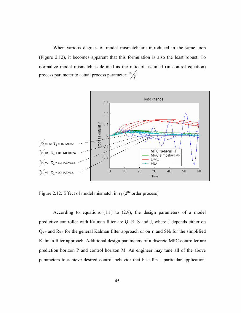
45

When various degrees of model mismatch are introduced in the same loop

(Figure 2.12), it becomes apparent that this formulation is also the least robust. To

normalize model mismatch is defined as the ratio of assumed (in control equation)

process parameter to actual process parameter: 1

1

ττ%

Figure 2.12: Effect of model mismatch in τ1 (2nd order process)

According to equations (1.1) to (2.9), the design parameters of a model

predictive controller with Kalman filter are Q, R, S and J, where J depends either on

QKF and RKF for the general Kalman filter approach or on τi and SNi for the simplified

Kalman filter approach. Additional design parameters of a discrete MPC controller are

prediction horizon P and control horizon M. An engineer may tune all of the above

parameters to achieve desired control behavior that best fits a particular application.

=1: τ1 = 30; IAE=0.24

=2: τ1 = 60; IAE=0.65

=3: τ1 = 90; IAE=0.8

=0.5: τ1 = 15; IAE=2 1

1

ττ%

1

1

ττ%

1

1

ττ%

1

1

ττ%

Time

46

The most frequently tuned parameters are the penalties (Q, R, S). They are normally

tuned with process restrictions, such as different speeds of control or known model

mismatch, in mind. In an industrial plant unit, different manipulated variables may have

different requirements with respect to how fast they react to a setpoint change or a

process disturbance. In some cases, variables are intentionally “clamped down” in order

to remove oscillation from large control elements. McMillan investigates the impact of

penalty tuning and gives an example of how to reduce overall variability by optimizing

a coarse valve / fine valve problem with MPC [28]. Figure 2.13 shows how different

values of R effect the control performance of three different single loop MPC

controllers (the PI response to the same stimulus is plotted for reference – R does not

apply).

Figure 2.13: Effect of move penalty R on the integral absolute error of different controllers subject to an unmeasured disturbance of 1. Process: K=1; τ1 =30s; τ2=20s; Θ =1; MPC: P=30; M=9; Q=1; PID: KC=52.5; Ti=28; Td=5.7 (Skogestad tuning)

All trends indicate that the smallest possible R will result in the smallest IAE,

and therefore the best control performance. This outcome makes sense because this

IAE

47

scenario has no model mismatch; increasing values of R will unnecessarily slow down

the reaction of the controllers to unmeasured disturbances. This outcome also makes it

obvious that the model predictive controller with general Kalman filter has the best

performance, while DMC has the worst. These results are rather intuitive, because

DMC does not have an observer that is matched to the process model dynamics GW as

described in 2.1.

If the model does not match the process, the effect of tuning the penalty changes

drastically as shown in Figure 2.14.

Figure 2.14: Effect of move penalty R in the presence of model mismatch on processes of different order. Process: K=1, τ1 =30, τ2=20s, Θ =1; PID: KC=52.5, Ti=28, Td=5.7 (Skogestad); MPC: P=30, M=9, Q=1

48

For model mismatch in gain, IAE becomes a convex function of R when a

Kalman filter is used. If the model mismatch is in time constant only, a different

relation appears. Dramatic differences are also visible between first and second order

processes. In most commercial MPC, controllers control horizon M and fix prediction

horizon P to a certain value that is designed to be the best tradeoff between control

performance and CPU usage for a specific implementation [32]. Figure 2.15 shows how

MPC performance varies for different values of control horizon.

Figure 2.15: Effect of Control Horizon to control performance with perfect model on the integral absolute error of different controllers exposed to an unmeasured disturbance of 1. Process: K=1; τ1 =30s; τ2=20s; Θ =1; MPC: P=30; M=9; Q=1; PID: KC=52.5; Ti=28; Td=5.7 (Skogestad tuning), DMC is off scale

If a perfect model can be assumed, the control performance of all examined

controllers increases when the size of the control horizon is increased. However, for

this single loop scenario the control performance settles fairly early and cannot be

improved any further if M is increased beyond 6. Multivariable processes with difficult

process interaction and higher order models require longer control horizons but settle

out in a very similar manner. When analyzing the prediction horizon P, one can observe

49

the same behavior (the resulting curve settles out at about P=10 in this example). While

the minimum acceptable control horizon depends strongly on the number and amount

of interaction of process variables, in a multivariable controller the minimum

acceptable prediction horizon depends on the deadtime to time constant ratio. When

MPC controllers are used in deadtime-dominant process applications, move blocking

may be used to artificially extend horizons in time [29]. Figure 2.16 shows the effect of

control horizon to control performance in the presence of model mismatch for first and

second order processes.

Figure 2.16: Effect of Control Horizon to control performance in the presence of model mismatch on processes of different order. Process: K=1, τ1 =30, τ2=20s, Θ =1; PID: KC=52.5, Ti=28, Td=5.7 (Skogestad); MPC: P=30, M=9, Q=1

50

As in the move penalty analysis, it becomes apparent that MPC with a general

Kalman filter has very little tolerance for model mismatch. With a model mismatch

ratio of 2, the control horizon has to be very small (1 or 2) to avoid oscillatory behavior,

as shown in Figure 2.15. This is much lower than one would have usually designed just

by looking at the behavior in Figure 2.15. The conclusion that can be drawn from this is

that the amount of model mismatch must be known before a controller is tuned. With

smaller model mismatch ratios (e.g., 1.5), larger values of M=3,4 were acceptable

before instability occurred (not shown in figure). An interesting side observation is that

DMC, the controller without an observer, performs better with model mismatch than

without it. In addition, it outperforms the other controllers when the model mismatch is

limited to the time constant. This fact suggests that not only the tuning, but also the

ideal type of Kalman filter can only be selected with knowledge of amount and type of

model mismatch (i.e., which model parameter). In Summary,

1. Optimal error and move penalties depend on which process parameter has

model mismatch (gain, time constants, delay).

2. Optimal horizons become longer with higher model order and shorter with

higher model mismatch.

3. Optimal tuning for first and second order processes is very different (including

optimal Kalman filter method).

4. Many relations shown in the plots above are convex functions, suggesting that

optimization algorithm could be used to find an optimum.

The next chapter describes how optimal tuning can be found using a solver for

situations with and without model mismatch.

51

Chapter 3

Optimal control in the presence of model mismatch

As discussed in section 1.4, tuning parameters for model predictive controllers

are commonly used to adjust the controller behavior in a way that is desirable for a

particular plant application. For example, a certain desired speed of response may be set

by tuning the move penalties R to a certain value. However, the expected behavior that

is designed by the commissioning engineer will only occur if the model mismatch is

insignificant, which is rarely the case in industrial plants. To account for the apparent

model mismatch, practitioners often resort to iterative tuning until the desired behavior

can be observed. This process is costly because it is very time-consuming, and it is

difficult to cover all control and constraint scenarios on a running plant. Even if this

method results in the desired plant behavior for the given model mismatch, one can

expect the behavior to change if the magnitude of model mismatch changes.

Furthermore, even if the amount of model mismatch and its variation is known, today

there is no method to derive tuning from this information. This chapter shows how

knowledge of model mismatch can be used to determine tuning for optimal control

performance in the presence of constant or changing model mismatch. Even though

some practitioners have tried to address this problem with empirical methods [8], it is

rarely addressed in control literature because textbook control theory is usually derived

for perfect models only.

3.1 Calculation of optimal tuning

In section 2.4, the effect of the most common MPC tuning parameters were

discussed and documented. As was shown above, the way in which tuning parameters

52

influence the MPC control behavior and closed-loop control performance depends on

the amount of model mismatch. In some cases, relationships are very significant and/or

nonlinear. The following MPC tuning and design parameters will be used for further

analysis:

• MPC controller tuning:

o P (prediction horizon), integer

o M (control horizon), integer

o QMPC (move penalty), float vector

o RMPC (error penalty), float vector

• Type of Kalman Filter (TKF): General or Simplified, boolean

• Kalman filter tuning

o General

QKF (covariance of the disturbances in w), float matrix

RKF (covariance of the measurement noise, z) , float matrix

o Simplified

T (filter time constants τi, float vector

SNR (signal-to-noise ratio for each disturbance), float vector

Different implementations of MPC may use additional tuning parameters, such

as maximum move rate or reference trajectory [32]. However, such parameters are

usually intended for specific needs of operators, and the resulting effects overlap with

the above mentioned parameters. Even though other means of influencing the dynamic

behavior of MPC exist, the majority of desired behavior can be addressed with the

parameters described in this work.

53

Since model mismatch and the tuning parameters are highly correlated with

respect to the closed-loop control performance, an optimization problem with

constraints was formulated. Figure 3.1 shows a schematic overview of the problem to

be solved: based on knowledge of model mismatch and change in model mismatch,

ideal tuning parameters shall be derived.

Figure 3.1: Schematic overview of optimization method: MPC tuning and design parameters are calculated based on model parameters and model mismatch

It is to be expected that the optimal set of tuning parameters for a given model

mismatch is suboptimal for the scenario in which no model mismatch is present.

Constraints have been added to the optimization to address physical and logical

boundaries in an arbitrary way. As will be seen later, the exact value of the constraints

influences only the range of calculation, not the overall result. The optimization

problem can be represented as:

min Γ, Ξ, Ξ Ξ

s.t. g Γ 0 (3.1)

where Γ =[P,M,QMPC,RMPC,TKF,QKF,RKF,T,SNR]T, Ξ =[G, τ1, τ2]T, g Γ are

inequality constraints describing computational limits of the control algorithm and IAE

is the control performance as introduced in Chapter 1. Figure 3.2 shows the best

possible IAE for a given amount of model mismatch in process model gain, obtained by

solving this optimization problem for different values of model mismatch. The detailed

min IAE(x)

TKF, QKF,RKF / T,SNR

QMPC, RMPC

M, P

Model

Model mismatch

54

optimization results are shown in Table 3.1. Active constraints are shown in bold. One

can observe that the optimizer makes use of all tuning parameters to achieve the

optimal control performance. It computes different tuning parameters for different

values of model mismatch that result in fairly similar control performance, as long as

no constraint is reached. Whenever a constraint is reached, the control performance

suffers because the optimizer runs out of degrees of freedom (i.e., tuning parameters) to

compensate for model mismatch. It also becomes apparent that MPC with general

Kalman filter outperforms MPC with simplified Kalman filter if K>K, and MPC with

simplified Kalman should be chosen if K<K. As seen in 2.1, the general Kalman filter

formulation is more rigorous than that of the simplified Kalman filter, which uses

EWMA filtering to update the state variable; thus, it cannot be tuned to deal with

smaller-than-expected gain very well, but excels with larger-than-expected gain. Since

MPC with simplified Kalman filter is based on filtering (section 2.1), it is more robust

than MPC with general Kalman filter if the process response has a smaller than

expected magnitude (K<K). However, for K>K it produces a slightly higher integral

absolute error than MPC with a general Kalman filter.

Note that the optimization method suggests relatively discontinues targets for Γ, the independent variables, for some values of Ξ Ξ, the model mismatch. This is most

likely caused by presence of multiple local optima to which the particular nonlinear

solver algorithm of this example implementation converges. No further investigation of

different solvers or different solver settings was done because the same optima were

found reproducibly in multiple runs and the resulting IAE values were already

satisfactory and sufficiently continuous.

55

Figure 3.2 Optimal tuning of model mismatch in process gain

General Kalman Filter Simplified Kalman filter Model

Mismatch IAE RMPC P M QKF RKF IAE RMPC P M T SN

0.25 1.729 0.0001 3 1 1 0.001 0.478 0.0001 3 1 73.5067 30.0714 0.5 0.574 0.0001 3 1 1 0.001 0.215 0.0001 3 1 100 30.0916

0.75 0.236 0.0001 3 1 1 0.001 0.285 0.0001 3 1 20.3385 30.0104 1 0.123 0.0001 3 1 1 0.001 0.162 0.0001 4 1 100 30.0824

1.25 0.087 0.0001 3 1 1 0.001 0.085 0.0001 3 1 100 30.0788 1.5 0.081 0.0001 3 1 1 0.001 0.229 0.0001 3 1 12.6669 30.0055

1.75 0.107 0.0001 3 1 0.9946 0.0033 0.166 0.0095 15 6 100 30.0943 2 0.062 0.0001 12 6 1 0.0023 0.217 0.024 50 10 76.3204 30.1224

2.25 0.241 0.0001 3 1 1 0.0898 0.267 0.0424 23 19 100 30.048 2.5 0.087 0.0001 26 6 0.9974 0.0099 0.32 0.0769 15 16 100 30.2111

2.75 0.099 0.0001 27 6 0.9501 0.0182 18.182 0.01 27 11 10 30 3 0.111 0.0001 27 6 0.966 0.0312 16.667 0.01 27 11 10 30

3.25 0.123 0.0001 28 6 0.9355 0.047 15.385 0.01 27 11 10 30 3.5 0.135 0.0001 27 6 0.9981 0.0728 14.286 0.01 27 11 10 30

Table 3.1 Optimal tuning of model mismatch in process gain, active constraints are shown in bold

If the model mismatch is attributed to the first order time constant, the

difference in integral absolute error between the two Kalman filter methods becomes

more pronounced. As shown in Figure 3.3, if the process is more responsive than

expected (τ1<τ1), the IAE rises with a very steep slope because oscillation occurs.

Oscillation caused by τ1<τ1 in the time domain is depicted in Figure 2.12. Both methods

00.20.40.60.8

11.21.41.61.8

2

0 0.5 1 1.5 2 2.5

IE

Model mismatch in Gain (G/G~)

general KF

simplified KF

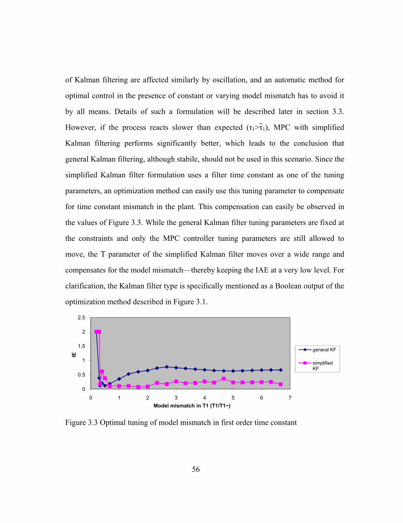
56

of Kalman filtering are affected similarly by oscillation, and an automatic method for

optimal control in the presence of constant or varying model mismatch has to avoid it

by all means. Details of such a formulation will be described later in section 3.3.

However, if the process reacts slower than expected (τ1>τ1), MPC with simplified

Kalman filtering performs significantly better, which leads to the conclusion that

general Kalman filtering, although stabile, should not be used in this scenario. Since the

simplified Kalman filter formulation uses a filter time constant as one of the tuning

parameters, an optimization method can easily use this tuning parameter to compensate

for time constant mismatch in the plant. This compensation can easily be observed in

the values of Figure 3.3. While the general Kalman filter tuning parameters are fixed at

the constraints and only the MPC controller tuning parameters are still allowed to

move, the T parameter of the simplified Kalman filter moves over a wide range and

compensates for the model mismatch—thereby keeping the IAE at a very low level. For

clarification, the Kalman filter type is specifically mentioned as a Boolean output of the

optimization method described in Figure 3.1.

Figure 3.3 Optimal tuning of model mismatch in first order time constant

0

0.5

1

1.5

2

2.5

0 1 2 3 4 5 6 7

IE

Model mismatch in T1 (T1/T1~)

general KF

simplified KF

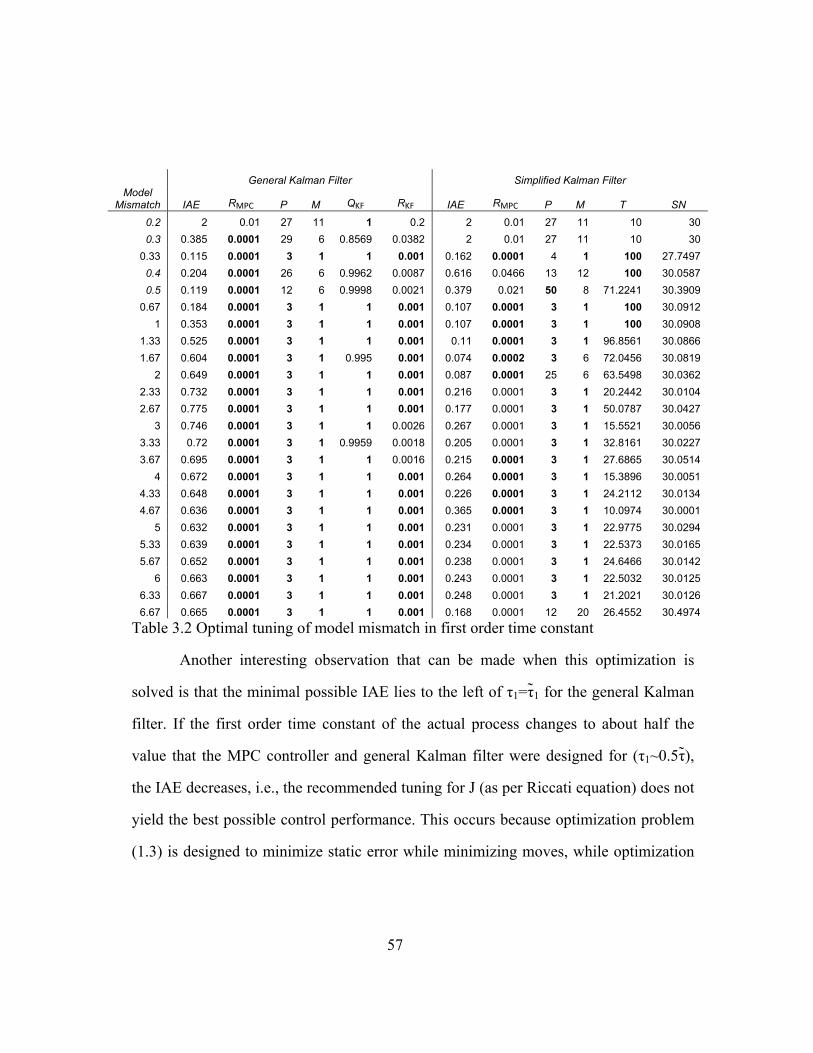
57

General Kalman Filter Simplified Kalman Filter

Model Mismatch IAE RMPC P M QKF RKF IAE RMPC P M T SN

0.2 2 0.01 27 11 1 0.2 2 0.01 27 11 10 30 0.3 0.385 0.0001 29 6 0.8569 0.0382 2 0.01 27 11 10 30

0.33 0.115 0.0001 3 1 1 0.001 0.162 0.0001 4 1 100 27.7497 0.4 0.204 0.0001 26 6 0.9962 0.0087 0.616 0.0466 13 12 100 30.0587 0.5 0.119 0.0001 12 6 0.9998 0.0021 0.379 0.021 50 8 71.2241 30.3909

0.67 0.184 0.0001 3 1 1 0.001 0.107 0.0001 3 1 100 30.0912 1 0.353 0.0001 3 1 1 0.001 0.107 0.0001 3 1 100 30.0908

1.33 0.525 0.0001 3 1 1 0.001 0.11 0.0001 3 1 96.8561 30.0866 1.67 0.604 0.0001 3 1 0.995 0.001 0.074 0.0002 3 6 72.0456 30.0819

2 0.649 0.0001 3 1 1 0.001 0.087 0.0001 25 6 63.5498 30.0362 2.33 0.732 0.0001 3 1 1 0.001 0.216 0.0001 3 1 20.2442 30.0104 2.67 0.775 0.0001 3 1 1 0.001 0.177 0.0001 3 1 50.0787 30.0427

3 0.746 0.0001 3 1 1 0.0026 0.267 0.0001 3 1 15.5521 30.0056 3.33 0.72 0.0001 3 1 0.9959 0.0018 0.205 0.0001 3 1 32.8161 30.0227 3.67 0.695 0.0001 3 1 1 0.0016 0.215 0.0001 3 1 27.6865 30.0514

4 0.672 0.0001 3 1 1 0.001 0.264 0.0001 3 1 15.3896 30.0051 4.33 0.648 0.0001 3 1 1 0.001 0.226 0.0001 3 1 24.2112 30.0134 4.67 0.636 0.0001 3 1 1 0.001 0.365 0.0001 3 1 10.0974 30.0001

5 0.632 0.0001 3 1 1 0.001 0.231 0.0001 3 1 22.9775 30.0294 5.33 0.639 0.0001 3 1 1 0.001 0.234 0.0001 3 1 22.5373 30.0165 5.67 0.652 0.0001 3 1 1 0.001 0.238 0.0001 3 1 24.6466 30.0142

6 0.663 0.0001 3 1 1 0.001 0.243 0.0001 3 1 22.5032 30.0125 6.33 0.667 0.0001 3 1 1 0.001 0.248 0.0001 3 1 21.2021 30.0126 6.67 0.665 0.0001 3 1 1 0.001 0.168 0.0001 12 20 26.4552 30.4974

Table 3.2 Optimal tuning of model mismatch in first order time constant

Another interesting observation that can be made when this optimization is

solved is that the minimal possible IAE lies to the left of τ1=τ1 for the general Kalman

filter. If the first order time constant of the actual process changes to about half the

value that the MPC controller and general Kalman filter were designed for (τ1~0.5τ),

the IAE decreases, i.e., the recommended tuning for J (as per Riccati equation) does not

yield the best possible control performance. This occurs because optimization problem

(1.3) is designed to minimize static error while minimizing moves, while optimization

58

problem (3.1) is designed to minimize the IAE, thereby maximizing control

performance.

The effect of model mismatch in the second order time constant shown in

Figure 3.4 is very similar to that of model mismatch in the first order time constant

shown above. The magnitude of the differences between general and simplified Kalman

filters is smaller, however, the trend is the same.

Figure 3.4 Optimal tuning of model mismatch in second order time constant

General Kalman Filter Simplified Kalman Filter

Model mismatch IAE RMPC P M QKF RKF IAE RMPC P M T SN

0.25 2 1.5182 44 6 1 0.001 3 0.01 27 11 10 30 0.3 0.37 0.0001 28 6 0.9454 0.0382 3 0.01 27 11 10 30 0.4 0.199 0.0001 30 6 0.996 0.0082 0.567 0.0404 12 12 85.7026 30.1881 0.5 0.116 0.0001 13 6 0.9971 0.0018 0.367 0.0176 29 8 100 30.434 0.6 0.151 0.0001 3 1 0.9918 0.0018 0.234 0.007 32 6 89.8552 30.1182 0.7 0.112 0.0001 3 1 1 0.001 0.161 0.0001 4 1 100 30.0948

0.75 0.11 0.0001 3 1 1 0.001 0.107 0.0001 3 1 100 30.0913 0.8 0.11 0.0001 3 1 1 0.001 0.215 0.0001 3 1 20.2633 30.0103 0.9 0.112 0.0001 3 1 1 0.001 0.215 0.0001 3 1 20.2576 30.0103

1 0.123 0.0001 3 1 1 0.001 0.162 0.0001 4 1 100 30.0824 1.25 0.169 0.0001 3 1 1 0.001 0.215 0.0001 3 1 20.2556 30.0103

1.5 0.229 0.0001 3 1 1 0.001 0.107 0.0001 3 1 100 30.0911 1.75 0.294 0.0001 3 1 1 0.001 0.107 0.0001 3 1 100 30.0912

2 0.353 0.0001 3 1 1 0.001 0.107 0.0001 3 1 100 30.0908 2.25 0.412 0.0001 3 1 1 0.001 0.108 0.0001 3 1 100 30.0908

2.5 0.478 0.0001 3 1 1 0.001 0.109 0.0001 3 1 100 30.0908

0

0.5

1

1.5

2

2.5

3

3.5

-0.25 0.25 0.75 1.25 1.75 2.25 2.75 3.25 3.75

IE

Model mismatch in T2 (T2/T2~)

general KF

simplified KF

59

2.75 0.527 0.0001 3 1 1 0.001 0.111 0.0001 3 1 81.9354 30.0729 3 0.559 0.0001 3 1 1 0.001 0.116 0.0001 3 1 71.5816 30.0626

3.25 0.577 0.0001 3 1 1 0.0011 0.122 0.0001 3 1 74.8502 30.0667 3.5 0.591 0.0001 3 1 1 0.001 0.128 0.0001 3 1 62.3478 30.0663

3.75 0.605 0.0001 3 1 1 0.001 0.134 0.0001 3 1 58.3664 30.0445 Table 3.3 Optimal tuning of model mismatch in second order time constant

This section discussed how optimal tuning parameters for MPC control and

state update can be obtained from knowledge about model and model mismatch by

using optimization. The actual calculations and MATLAB implementation that was

used for the examples above are shown in Appendix A. The impact of model mismatch

and optimal tuning to compensate for it were analyzed by each model parameter

separately. In a real plant scenario, all parameters that correspond to a prescribed model

(and others that are not modeled for various reasons) will vary simultaneously. Which

model parameter is most affected depends mainly on process type and cause of model

mismatch (e.g., tube fouling, varying heat coefficient of fuel). Depending on the model

identification method, a model mismatch in lead time constant may be interpreted as

model mismatch in model deadtime or time constant. Often, one or two model

parameters contribute significantly to model mismatch simultaneously. The next

section analyzes model mismatch in multidimensional subspace.

3.2 Optimal tuning map

This section analyzes the effects of model mismatch in more than one model

parameter and shows how optimal tuning can be calculated. Figure 3.5 depicts a surface

plot of best possible IAE as calculated by optimization (3.1) shown in the previous

section. Gain and first order time constants are allowed to have model mismatch. The

optimal tuning for model mismatch in first order time constant and second order time

constant are very similar, with the first order time constant being more significant (see

60

also Figure 3.3 and Figure 3.4); therefore three-dimensional visualization is preferred

over four-dimensional, and the effects of model mismatch in second order time constant

have been neglected in this plot.

Figure 3.5: Optimal tuning map for model mismatch in K and τ1 of MPC with general Kalman filter state update

For easier visibility the values of K/K=1 and τ1/τ1=1 are indicated as lines. The

point where the lines intersect represents control performance with a perfect model. The

cross section along each line exactly represents the plots in Figure 3.2 and Figure 3.3,

respectively. As discussed previously, model mismatch in time constant in the direction

of τ1<τ1 leads to oscillatory behavior; however, one can see that this oscillation does not

occur if there is model mismatch in gain K<K at the same time. As expected, with

model mismatch in gain K>K the problem gets worse. The fact that model mismatch in

inherently different model parameters can cancel out or amplify the overall effects on

control performance shows that it is important to evaluate all dimensions of model

mismatch during calculation of optimal controller and state update tuning. It also

61

becomes apparent that the best control performance is not necessarily achieved with the

perfect model. If K/K=2 and τ1/τ1=1.5, the control performance is 0.0545 instead of

0.1226 at K/K=1 and τ1/τ1=1, a 56% improvement, assuming that the tuning parameters

are optimally calculated by the described optimization formulation.

If the assumed process model and the exact process model mismatch were

known, the model used by the controller and observer could obviously be substituted

with a perfect model to achieve an even better performance. However, since this

research is aimed towards deriving a method that does not depend on an exact process

model, the discussed results are achieved by only adjusting the tuning parameters

defined in 3.1 and leaving the assumed process model unchanged (as this would be the

best guess of an engineer in a plant).

Figure 3.6 depicts the equivalent tuning map for MPC with simplified Kalman

filtering. The top left corner of both optimal tuning maps indicates a region of

instability; both plots are cut off at IAE=2. It is obvious that this region is approached

with a very steep slope. Calculating and plotting 3-dimensional tuning maps allows

easy assessment of size, location, and steepness of such unstable region(s). Since such

regions should be avoided by all means, constraints for highly penalized slack variables

can be added into the optimization problem. When comparing the optimal tuning maps

of MPC with the different Kalman filter methods, it becomes apparent that both

controllers become unstable in region τ1>τ1, K<K. But only the MPC with a general

Kalman filter becomes unstable in region [τ1<τ1, K>K]. As suggested previously, the

inherent filtering that is found only in the simplified Kalman filter acts as a stabilizing

mechanism.

Figsim

map

Pro

cess

gai

n K

0

2Tabgen

gure 3.6: Optmplified Kalm

The det

ps are shown

0.25 .25 0.493 0.3 0.389 0.4 0.298 0.5 0.222 0.6 0.293 0.7 0.362 0.8 0.429

1 0.556 1.2 41.6667 1.5 33.3333

2 25 2.5 20 ble 3.4 Optimneral Kalman

I

timal tuning man filter sta

tailed perform

n in Table 3

0.3 0.540 0.0.407 0.0.282 0.0.273 0.0.188 0.0.239 0.0.290 0.0.385 0.

0.4765 0.233.3333 0.6

25 20

mal tuning mn filter state

01.

20.000

0.500

1.000

1.500

2.000

m

E

map for moate update

mance and t

.4 and Table

0.4 0.5 711 0.929 505 0.654 302 0.368 225 0.241 190 0.186 238 0.158 146 0.168 205 0.119 619 0.157 397 0.2132

25 25 20 20

map results foupdate. This

0. 25

0. 4

0. 6

0. 82

0.2mmG

62

odel mismatc

tuning param

e 3.5.

Process tim

0.6 01.150 1.320.823 0.990.463 0.560.289 0.350.201 0.230.159 0.170.138 0.130.155 0.11

0.1004 0.1420.1409 0.2040.3322 0.146

20 0.193for model mis table corre

250.5

0.8

ch in K and τ

meter values

me constant τ1

.7 0.8 26 1.461 197 1.140 167 0.674 054 0.427 037 0.285 073 0.202 039 0.152 012 0.109 021 0.0998 043 0.0686 65 0.1069 035 0.2208 0ismatch in Ksponds with

1.5

τ1 of MPC w

s for the disc

1 1.21.7294 1.93991.3334 1.51610.8897 1.02830.5737 0.72630.3934 0.49980.2774 0.36250.2027 0.26720.1226 0.15720.0903 0.1029

0.081 0.07210.0617 0.08330.0867 0.1187

K and τ1 of Mh Figure 3.5.

mmT

with

cussed tunin

2 1.5 9 1.9782 1.8

1.7235 1.63 1.1634 1.33 0.873 1.08 0.6621 0.75 0.4833 0.62 0.3666 0.52 0.2218 0.39 0.142 0.2

0.0833 0.13 0.0545 0.07 0.0678 0.0

MPC with

ng

2 2.5 8572 1.8868 6796 1.5898 3821 1.3515 0173 1.1526 7949 0.9016 6528 0.7192 5261 0.6114 3308 0.4364 2228 0.297 1282 0.1835 0632 0.0891 0318 0.051

63

Process time constant τ1

0.25 0.3 0.4 0.5 0.6 0.7 0.8 1 1.2 1.5 2 2.5

Pro

cess

gai

n K

0.25 0.622 0.622 0.631 0.431 0.432 0.431 0.435 0.478 0.5267 0.5995 0.7038 0.5233 0.3 0.232 0.356 0.522 0.534 0.359 0.377 0.360 0.3722 0.4077 0.4837 0.8559 0.5504 0.4 1.341 0.266 0.395 0.395 0.424 0.424 0.269 0.4083 0.2733 0.303 0.3617 0.6488 0.5 0.656 0.428 0.341 0.317 0.317 0.317 0.318 0.2152 0.2163 0.2212 0.2563 0.2906 0.6 0.787 0.564 0.595 0.269 0.178 0.265 0.265 0.2848 0.1794 0.2764 0.1945 0.2844 0.7 0.921 0.695 0.571 0.165 0.152 0.152 0.305 0.3056 0.1529 0.1542 0.1571 0.1748 0.8 62.500 0.783 0.935 0.258 0.133 0.268 0.268 0.1333 0.1334 0.268 0.1355 0.1432

1 50.000 50.000 0.616 0.379 0.240 0.152 0.215 0.1615 0.1065 0.1067 0.1077 0.1085 1.2 41.6667 41.6667 41.6667 0.5047 0.3312 0.2191 0.1313 0.0886 0.0886 0.0888 0.089 0.0899 1.5 33.3333 33.3333 33.3333 33.3333 0.4534 0.336 0.2269 0.2287 0.0708 0.0709 0.071 0.0712

2 25 25 25 25 25 25 0.5084 0.2171 0.2024 0.0533 0.0532 0.0809 2.5 20 20 20 20 20 20 20 0.3197 0.2016 0.1033 0.0425 0.0863

Table 3.5 Optimal tuning map results for model mismatch in K and τ1 of MPC with simplified Kalman filter state update. This table corresponds with Figure 3.6.

3.3 Addressing varying model mismatch

As shown in the previous sections, the optimization problem (3.1) computes the

optimal tuning for a particular value of model mismatch, which is one of the original

goals of this research. This optimal tuning map is useful for calculating MPC and

observer tuning that will ensure optimal control performance. As discussed in the first

chapter, industrial users of MPC usually have to manually adjust tuning “knobs” until a

desired behavior appears to be reached because such a method was not available before.

However, while it is easier to determine the presence of model mismatch than the

correct model, one could argue that it may still be difficult to determine the specific

amount of model mismatch. Although determining the amount of model mismatch may

still be easier than determining the precise model because it requires less process

perturbation, the amount of model mismatch may change over time. For these reasons a

more feasible and easier to determine measure than model mismatch is the range of

64

model mismatch. An example of a range of model mismatch in a two dimensional

subspace (ignoring the second order time constant as done above) may be written as

Kactual=2±0.5 and Tactual=20s±5s and illustrated in 3-dimensional subspace as depicted

in Figure 3.7. Once model mismatch is defined in this way it can be overlaid with the

optimal tuning map described above.

Figure 3.7: Illustration of two-dimensional model mismatch subspace example with Kactual=2±0.5 and Tactual=20s±5s

Such overlay can then be implemented in a software package that displays it to

the engineer. This can be very useful to the engineer as he/she commissions the

controller because then he/she can assess the worst and best possible control

performance as a function of model mismatch for a particular tuning and make manual

corrections. An example view of the overlay is shown in Figure 3.8.

Δτ=10sΔK=1

65

Figure 3.8: Illustration of two-dimensional model mismatch example with Kactual=2±0.5 and Tactual=20s±5s

In this example, the worst control performance occurs if Kactual=1.5 and

Tactual=25s. However, the IAE at that point is 0.7, which could be considered by the

engineer to be acceptable regardless, especially since the likelihood of being within that

region is relatively low because only a small surface area overlaps with IAE values

above 0.5. If more knowledge about the model mismatch was available (e.g., physical

process limitations), then the two-dimensional model mismatch subspace as depicted in

Figure 3.7 could be modified to account for likelihood of occurrence. Oval and other

shapes are conceivable instead of the depicted rectangle.

66

3.4 Closed-loop performance improvements from tuning of model parameters

Previous sections showed how the methodology, suggested in this research can

determine the most ideal tuning for a given model and model mismatch range. In this

work tuning is defined clearly as the MPC controller and observer parameters described

in (3.1). However, looking at Figure 3.8, it becomes clear that calculated tuning does

not necessarily provide the lowest possible IAE because the center point of the model

mismatch subspace is fixed at the assumed “perfect” model. If this subspace, which in

this two-dimensional example is represented by a surface, was allowed to move, it

could most likely find a lower value for the worst IAE within the surface, thereby

increasing the overall control performance.

Figure 3.9: Schematic overview of revised optimization method: MPC tuning and design parameters are calculated based on model and model mismatch range

67

As mentioned previously, this research intentionally does not update the

assumed model with knowledge about model mismatch because the result may be as

uncertain as the assumed model in the first place. However, as depicted in Figure 3.9,

the model used for calculating the MPC control moves may be modified as the

described model mismatch surface is relocated within the tuning map. The minimal

possible value of the worst IAE within the model mismatch subspace can be found by

formulating and solving a second optimization problem.

min max Ξ Ξ , Ψ

s.t. g Γ 0 (3.2)

where Ψ is the tuning map calculated by iterating (3.1) over arbitrary

combinations of model mismatch and g Γ are inequality constraints describing the

dimensions of tuning map Ψ . It should be noted that no additional process model

knowledge is required for this operation because the tuning map is still built based on

the model provided by the engineer (the assumed model). The result of the optimization

is a modified model that is subsequently used to develop the MPC controller. The

tuning map is not recalculated based on the new model because its sole purpose is to

minimize IAE within the current tuning map. By adding this operation to the method,

the model parameters of the controller are tuned to the ideal values to maximize control

performance even further than possible with MPC and observer tuning. In a sense, the

model parameters have also become tuning parameters. If there was no model

mismatch, one would expect that the control performance of a controller with a

modified model would be worse than that of a controller with the original model.

However, as discussed above, the chance of that occurring is very small. In a real plant

scenario the performance of the original controller may be is worse than that of the

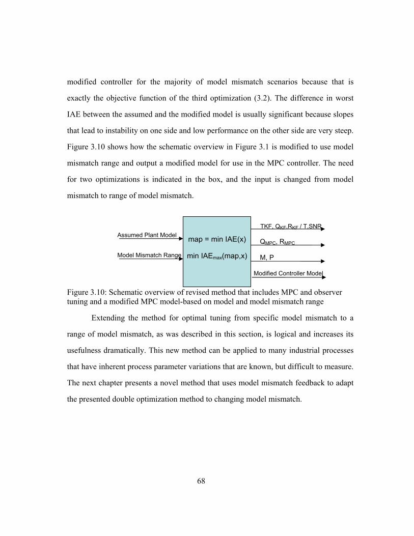
68

modified controller for the majority of model mismatch scenarios because that is

exactly the objective function of the third optimization (3.2). The difference in worst

IAE between the assumed and the modified model is usually significant because slopes

that lead to instability on one side and low performance on the other side are very steep.

Figure 3.10 shows how the schematic overview in Figure 3.1 is modified to use model

mismatch range and output a modified model for use in the MPC controller. The need

for two optimizations is indicated in the box, and the input is changed from model

mismatch to range of model mismatch.

Figure 3.10: Schematic overview of revised method that includes MPC and observer tuning and a modified MPC model-based on model and model mismatch range

Extending the method for optimal tuning from specific model mismatch to a

range of model mismatch, as was described in this section, is logical and increases its

usefulness dramatically. This new method can be applied to many industrial processes

that have inherent process parameter variations that are known, but difficult to measure.

The next chapter presents a novel method that uses model mismatch feedback to adapt

the presented double optimization method to changing model mismatch.

map = min IAE(x)

min IAEmax(map,x)

TKF, QKF,RKF / T,SNR

QMPC, RMPC Assumed Plant Model

Model Mismatch Range

Modified Controller Model

M, P

69

Chapter 4

ovel method for closed-loop adaptive control

Most methods for adaptive control work by refining or re-creating a process

model continuously, or, if triggered by an event such as a change in process value or

operator setpoint, spontaneously. After a new model has been obtained, new controller

moves or tuning are calculated from it. A few methods adapt the tuning or other

controller parameters directly based on process information, without a model, e.g.,

identification-free algorithms developed by Maršik and Strejc [34]. Both groups of

methods rely on process variation that may be introduced by disturbances or setpoint

changes. The efficiency, precision and stability of these methods increase

proportionally with the amount of process variation.

Common engineering sense suggests that it is easier to determine the statistical

amount and variation of model mismatch than it is to determine/create a precise process

model. Many methods, such as autocorrelation, have been proposed to determine the

amount of model mismatch during closed-loop plant operations [33], [49], [52], [53]. It

is extremely difficult to determine a good process model during closed-loop plant

operation, however, because the controller objective (to minimize variation of product

quality) contradicts the requirement of model identification in order to maximize

variation in process outputs.

The method introduced in this chapter is novel because, as a logical

continuation of the findings in the previous chapter, it proposes to use the amount of

model mismatch to adjust the tuning parameters. While this method, like the one above,

70

depends on some amount of process variation, it does not need to maximize them in

order to derive the tuning that maximizes the control performance.

4.1 Analysis of innovation

The innovation (Ik), also referred to as the residuals or prediction error, is

defined as:

(4.1)

where yK is the predicted process output and is the actual value of the

process output. This term is used in the Kalman filter equation (2.8) to calculate the

updated state variable. Researchers have proposed many methods that analyze

innovation [33], [49]. Often the application of such methods occurs during the

commissioning or maintenance phase of a predictive control or soft sensor (e.g., neural

network) project. Autocorrelation, for instance, is a method that is frequently used

because it allows distinguishing between model error and unmeasured disturbance.

Since unmeasured disturbances manifest themselves in the same way as model error to

the operator—as the difference between the prediction and the actual value, i.e., a

nonzero innovation as seen in (4.1)—they are difficult to distinguish and can only be

corrected for by using feedback control.

Autocorrelation of the innovation provides an indication of how much of non-

random contributions are not removed from a signal during closed loop control. For a

discrete time series of length n {y1, y2, … yn} with known mean and variance, an

estimate of the autocorrelation can be obtained as:

)ˆky

var

cor

pro

con

then

var

extr

41%

pos

(ϭ=

eye

be e

Figoptpro

where R

riance, and

rrelated signa

oportion of w

ntroller tunin

n the tuning

Figure 4

riability (ϭ=6

ruder in a c

% reduction

ssible tuning

=4.0). This m

e. Only when

easily seen,

gure 4.1: Timtimal tuning,ocess noise, n

R(k) is the

is the me

als but not d

white noise

ng. If the pro

of the partic

4.1 shows th

6.8). The pre

chemical pla

in standard

g, the stand

makes it ver

n the autoco

as is shown

me Series of c, i.e. before anot tuning

Autocorrel

ean. Since a

disturbances

to correlate

ocess output

cular control

he controlle

esented data

ant. Retuning

deviation. A

ard deviatio

ry difficult t

rrelation plo

in Figure 4.

controlled vand after lam

71

lation that l

an optimally

s that are per

ed signal is

t of closed lo

ller is not op

d variable o

a was measu

g the contro

As can be se

on is still ve

o judge the

ots are comp

2.

ariable (presmbda tuning;

lies in the

y tuned con

rfectly rando

a good ind

oop control h

ptimal.

of a PID loo

ured on a pre

oller using la

een in this f

ery large fo

control perf

pared can the

ssure) of loo; most of the

range [-1,

ntroller can

om (i.e. whi

dication of

has large au

op with a re

essure contr

ambda tunin

figure, even

or this partic

formance w

e difference

op with subope variation is

(4.2

1], is th

only remov

ite noise), th

optimality o

utocorrelation

latively larg

rol loop of a

ng achieved

with the be

cular proces

ith the nake

in tuning ca

ptimal and

s due to

2)

he

ve

he

of

n,

ge

an

a

st

ss

ed

an

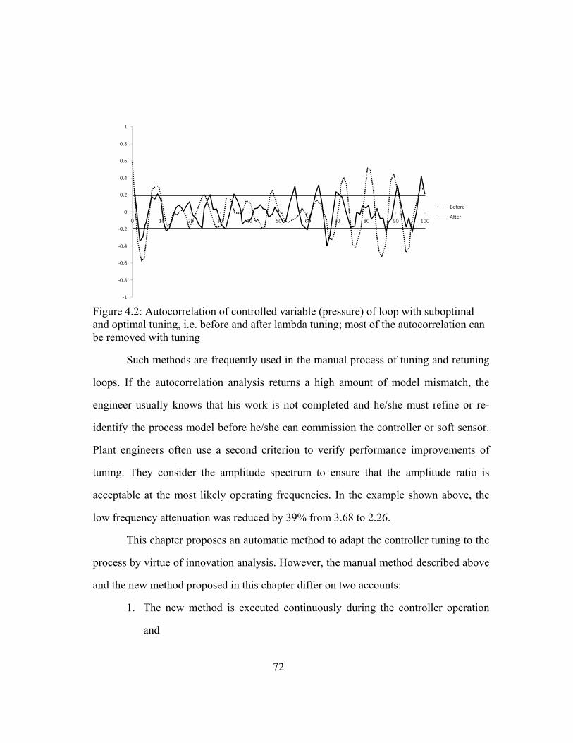
72

Figure 4.2: Autocorrelation of controlled variable (pressure) of loop with suboptimal and optimal tuning, i.e. before and after lambda tuning; most of the autocorrelation can be removed with tuning

Such methods are frequently used in the manual process of tuning and retuning

loops. If the autocorrelation analysis returns a high amount of model mismatch, the

engineer usually knows that his work is not completed and he/she must refine or re-

identify the process model before he/she can commission the controller or soft sensor.

Plant engineers often use a second criterion to verify performance improvements of

tuning. They consider the amplitude spectrum to ensure that the amplitude ratio is

acceptable at the most likely operating frequencies. In the example shown above, the

low frequency attenuation was reduced by 39% from 3.68 to 2.26.

This chapter proposes an automatic method to adapt the controller tuning to the

process by virtue of innovation analysis. However, the manual method described above

and the new method proposed in this chapter differ on two accounts:

1. The new method is executed continuously during the controller operation

and

73

2. In the new method the amount of model mismatch is not used to trigger a

model improvement, but to retune the controller to optimally account for the

new amount of model mismatch.

For model predictive controllers the controller output calculation is derived

directly from the process model. Therefore, autocorrelation can be attributed to model

mismatch.

Current practice in industrial process control deals with the combination of

model mismatch and unmeasured disturbance in innovation in a very basic way. DMC

controllers, for instance, assume a certain fraction of the innovation to be contributed

by unmeasured disturbances. The value can be configured and is usually between 0.5

and 0.8 [27], [32]. However, many researchers have shown this is very inefficient and

may lead to significant performance reduction and instability in non-minimum phase

systems. A more sophisticated way of selective control action for model mismatch and

unmeasured disturbances is the application of the Kalman filter. The Kalman filter is

formulated to specifically account for unmeasured disturbances that have a known

characteristic. However, this characteristic (covariance), as well as the process model,

is assumed to be known exactly. It is also not adaptive with respect to changes in the

fraction of unmeasured disturbances in the innovation because the fraction of model

mismatch in the innovation is assumed to be zero (since the model is assumed to be

known and constant). Han and Lin proposed a method of tuning the Kalman filter gain

based on autocorrelation of innovation [33]. This method tries to minimize the error

covariance seen by the Kalman filter by adapting the designed and actual signal-to-

noise ratios. This essentially maximizes the filter performance, which means that it not

necessarily maximizes the closed loop performance as discussed in previous chapters.

74

Unfortunately, this adaptive method only calculates the error covariances, and can only

be used if the perfect model is already known.

While autocorrelation is an indication of randomness in the signal, the R2

statistic gives an indication about how much of the variation on is explained by the

model:

1 1 (4.3)

where R2 is the R-squared value that lies in the range [0..1], is the variance,

and is the mean. As with autocorrelation, engineers use rules of thumb to determine

how much unaccounted variation is acceptable before a model has to be modified. R2

values above 0.8 are usually considered satisfactory. A value of 0.8 means that 20% of

the variation is unaccounted for by the model based prediction, which is very good if

achieved in a real plant scenario. However, if the model is over-parameterized, R2>0.8

may be misleading and a t-test is usually run to ensure the statistical significance of

each model parameter. The model can then be reduced by eliminating parameters that

turn out to be not statistically significant. The next section discusses how R2 may be

used to infer the approximate fraction of model mismatch versus unmeasured

disturbance that contributes to the prediction error.

4.2 Continuous model and tuning adaptation

Gain scheduling methods are very popular in industrial plants for processes with

changing process parameters. Such methods may schedule controller tuning as shown

by Maršik et al. [34], [35] or the process model and the tuning as shown by Thiele, et

75

al. [36] and Wojsznis et al. [37]. As long as the process parameters change

deterministically, satisfactory results can be achieved with such methods.

In industrial plants many feedstock and equipment properties are constantly

changing. Examples include change in BTU properties of fuel and change in

concentration of reagent. Other examples are discussed in the following section. If

measurable, the values of these property changes are frequently used in one of two

different ways:

1. By a feedforward strategy to directly reduce variation or

2. By a gain scheduling strategy to counteract modeling error and indirectly

cancel the impact.

Figure 4.3 shows how the optimal tuning method described in Chapter 3 can be

combined with an existing MPC controller and observer (indicated as “KF”) to create a

gain scheduling controller.

Figure 4.3: Application of optimal tuning method to MPC for manual tuning

If one or more process parameters of the model have changed and are known,

they can be updated in the “optimal MPC tuner”, which immediately retunes the

controller and Kalman filter to counteract negative downstream effects. The update can

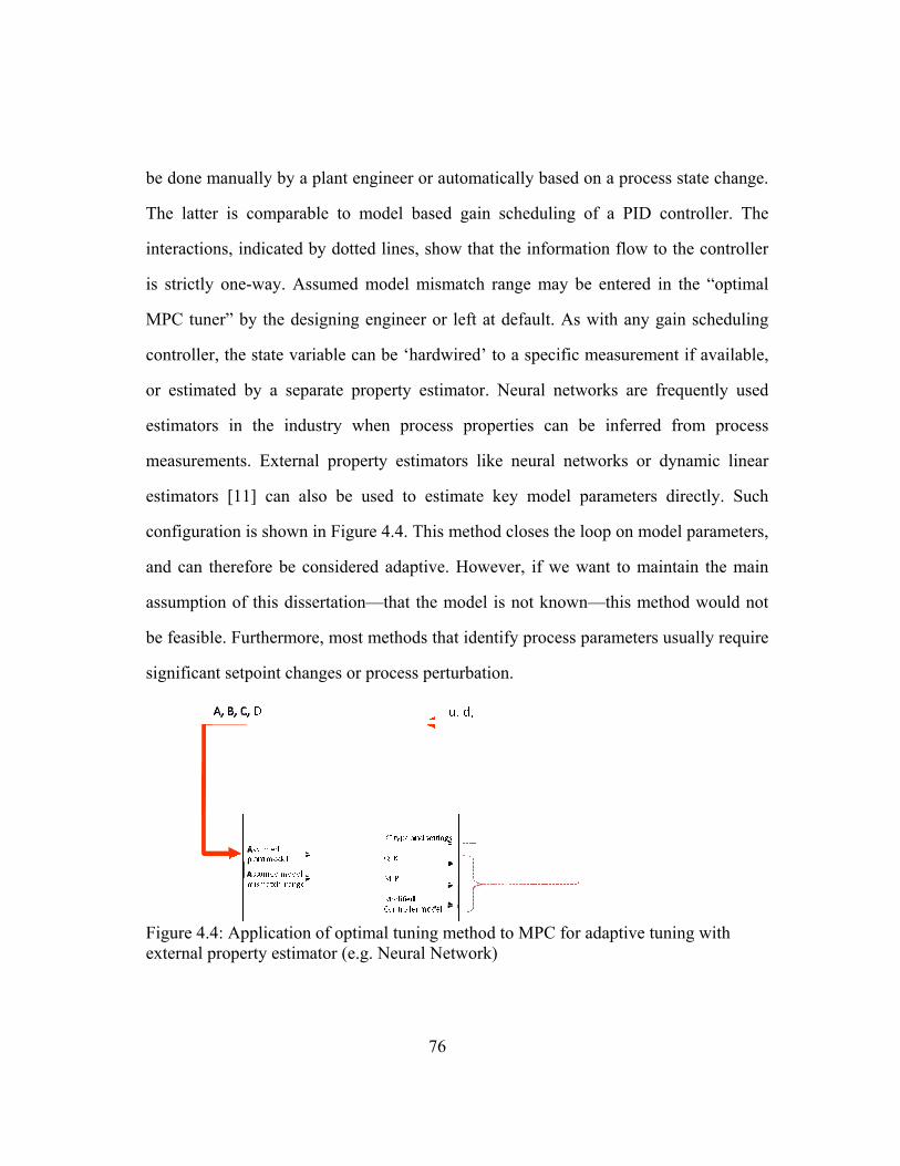
be d

The

inte

is s

MP

con

or

esti

mea

esti

con

and

assu

be f

sign

Figexte

done manua

e latter is c

eractions, in

strictly one-w

PC tuner” by

ntroller, the s

estimated b

imators in t

asurements.

imators [11]

nfiguration is

d can therefo

umption of

feasible. Fur

nificant setp

gure 4.4: Appernal proper

ally by a plan

comparable

dicated by d

way. Assum

y the design

state variabl

y a separate

the industry

External pr

] can also b

s shown in F

ore be consi

this disserta

rthermore, m

point changes

plication of orty estimator

nt engineer o

to model b

dotted lines,

med model m

ing engineer

le can be ‘ha

e property e

y when pro

roperty estim

be used to

Figure 4.4. T

idered adapt

ation—that th

most method

s or process

optimal tuninr (e.g. Neura

76

or automatic

ased gain s

show that th

mismatch ra

r or left at d

ardwired’ to

estimator. N

ocess proper

mators like

estimate ke

This method

tive. Howev

he model is

s that identif

perturbation

ng method tl Network)

cally based o

cheduling o

he informati

ange may be

default. As w

a specific m

Neural netwo

rties can be

neural netw

ey model pa

closes the lo

ver, if we wa

not known—

fy process p

n.

o MPC for a

on a process

of a PID co

ion flow to t

e entered in

with any gai

measuremen

orks are fre

e inferred f

works or dy

arameters d

oop on mode

ant to maint

—this metho

arameters us

adaptive tuni

state change

ontroller. Th

the controlle

the “optima

in schedulin

nt if available

equently use

from proces

ynamic linea

directly. Suc

el parameter

tain the mai

od would no

sually requir

ing with

e.

he

er

al

ng

e,

ed

ss

ar

ch

s,

in

ot

re

77

Estimators are usually connected to many variables, including those that are not

measured or manipulated by the control loop (shown in Figure 4.4). If the process

parameters change non-deterministically or the related state parameters cannot be

measured, adaptive tuning methods must be used in lieu of the model based adaptive

control discussed above. Examples include recursive model identification and model

switching [12], [13]. Figure 4.5 shows an overview of the most common techniques

used for adaptive control.

Figure 4.5: Adaptive control techniques

Since model based approaches are intentionally not considered in this research,

a large section of adaptive tuning techniques will not be considered. As can be seen in

Figure 4.5, model free approaches generally necessitate the modification of the control

formulation. The optimal MPC tuning method presented in Chapter 3 is similar in that

it only adjusts the MPC tuning parameters. The following analysis will focus on

developing a new method that estimates model mismatch without the need for model

identification.

78

Figure 4.6 shows a simple modification to the gain scheduling controller from

Figure 4.3 that enables adaptive control. The innovation, which is calculated in the

observer, is analyzed and processed by a method (shown as “innovation analysis”) that

will be discussed below. This “innovation analysis” is used to automatically update the

model mismatch range; all or part of the model mismatch range can be updated in this

way. Similarly, all or part of the parameters for which range is considered may be

modified, depending on how comprehensive the innovation method is with respect to

the number of model parameters. In other words, sometimes the innovation may only

allow conclusions to be made about a subset of the parameters in the actual model. If

that is the case, the range for the unknown parameters must be set conservatively to

include all model mismatch scenarios. The output of the optimal MPC tuner functions

in the same way as described in the on-demand update cases above, but closes the

adaptation loop in this scenario. The uniqueness of this adaptive control approach is

that the originally assumed model is never modified by the mechanism, preventing

runaway process identification, increasing robustness, and simplifying gain scheduling.

If desired, the assumed process model can be updated manually at any time without

having to stop or reset the adaptation. This is another advantage over current state of

the art adaptive methods. A trigger for manual or automatic model update can be easily

derived from the value of innovation or model mismatch range (i.e. either from the

input or the output of the “innovation analysis” component).

Figesti

cau

mag

of

com

sma

sen

erro

actu

gure 4.6: Appimator (with

Badwe

uses for inn

gnitude betw

the designe

mpared to em

all gain theo

The rel

nsitivity.

Badwe

or (4.5), con

ual loops:

plication of ohout need for

et al. [49] p

novation. Th

ween disturb

ed sensitivit

mpirically d

orem [50] are

lative sensit

et al. also s

ntroller outp

optimal tuninr property es

propose a m

his methodo

bances and m

ty Sd and

derived thres

e used to rule

tivity is th

show that it

ut (4.6) and

79

ng method tstimation)

method for d

logy gives

model misma

the relative

sholds. Addi

e out tuning

e ratio betw

relative sen

d spectral de

o MPC for a

distinguishin

an indicatio

atch. Frequen

e sensitivity

itionally, sta

problems.

ween the d

s itivity can

ensity ratios

adaptive tuni

ng between d

on of the d

ncy domain

y S∆ are ca

ability measu

designed an

n be used to

(4.7) of des

ing with stat

different roo

differences i

characteristi

alculated an

ures from th

nd the actua

(4.4

calculate th

signed versu

(4.5

(4.6

te

ot

in

ic

nd

he

al

4)

he

us

5)

6)

80

| ∆ | (4.7)

If the frequency response | ∆ | is known, the condition for marginal

stability ∆ 1 can be used to detect model mismatch. Unfortunately, this

calculation requires the identification of an updated process model. Since the initial

goal of this dissertation is to develop a controller tuning method that compensates for

model error without the need for model identification, the two cited methods cannot be

utilized. Methods that calculate model mismatch based on the comparison between two

models are usually theoretical methods and not realistic in a plant environment. An

“actual” plant model is only hypothetical since it cannot be more accurate than the

model that is already assumed to be the process model. Other methods have been

proposed to determine performance degradation due to model mismatch or other

causes. The cross-correlation test by Stanfelj et al. [51] uses the cross-correlation

between setpoint variations and internal model control error to discriminate between

process model error and disturbance model error. However, it requires SP perturbations

to the system and is designed for single loop controllers.

The autocorrelation of the innovation method described in the previous section

provides a model-free and perturbation-less alternative. As discussed above,

autocorrelation analysis can determine whether a loop’s control performance can be

improved or not without the need to identify a process model. Kesavan & Lee [52]

argue the same point but from a different perspective. In their work on diagnostic tools,

they compare autocorrelation of innovation before and after detuning a model based

controller in order to determine whether model mismatch is present or not. If model

mismatch is present, then two different controller tuning settings will result in different

81

autocorrelations. Currently this is a manual process. Such two process control scenarios

can be created by either running with two sets of controller tunings for two periods of

time, or by turning control off for some amount of time (open loop measurement).

Automating this method fully requires solving many challenges that are not part of this

dissertation research. Besides, as is the case with all well-defined safety nets, the

controller operation must be very transparent to the user. Even with safety nets fully

automated, the calculation of model mismatch using this particular method may still be

too disruptive and impractical for some types of processes or plants. Further research

like that discussed in section 2.4 needs to be done on this method of two tuning

scenarios to understand the effects of different types of model parameters and their

interactions. Furthermore, it has yet to be determined how much the tuning settings

have to differ in order to see significant differences and what the impact of the number

of samples (test duration) in each tuning scenario on the overall confidence is. The

following section discusses the results from experimental test runs of a model

predictive controller that uses the optimal tuning method described in this chapter

(Figure 4.6) using a practical approximation to estimate model mismatch from

autocorrelation of innovation.

4.3 Case study: Level loop in distillation column process

To verify the concepts presented in Chapter 3 and Chapter 4, the proposed

tuning methods were applied to a binary distillation column. This particular column is a

pilot plant of smaller than average scale that is used to separate water and ethanol. The

process and instrumentation diagram is shown in Figure 4.7.

82

Figure 4.7: P&ID of binary distillation column used for experimental testing of proposed methods

Since the flow out of the accumulator can be measured, a cascade strategy was

chosen that allows separating the fast flow and the slow integrating level dynamics.

This separation between level control (LIC-091) and flow control (FIC-100) generally

increases robustness. However, both controllers must be tuned fairly well for this effect

to be realized. This is a challenging task in this plant because the process parameters

change as the column energy input varies. Since steam flow is used to control the

bottoms temperature in order to control the purity, the process parameters of level and

83

flow control loops in the accumulator can change significantly during normal operation.

Manual step testing was performed to determine the process model at a steam flow of

0.55 kg/min. The step test yielded the following initial model, which will be used as the

assumed model for the model based controllers and will provide initial tuning for the

PID controllers: . . ; . . . (At steam =

0.4 kg/min: . ). Even though these models are FOPDT, they

were used for further analysis of the level loop. This approximation of an integrating

process with a FOPDT model was done intentionally to guarantee model mismatch

during the experiments. Some commonly used tuning rules, such as Ziegler-Nichols,

will result in the same PID tuning anyway because they are solely based on ultimate

gain, ultimate period and deadtime. Practitioners often try both model types on

integrating processes to see which performs better and/or is more robust.

For the experiments the level controller LIC-091, which is normally a PID

controller was replaced with MPC control that was executed in MATLAB. This was

implemented by leaving the PID controller in manual mode and sending OPC writes

from an OPC client on the laptop computer to the outputs of the PID controller in the

DeltaV system. Figure 4.8 shows how the open standard OPC protocol is used to

read/write access real-time plant data, which is owned by the control system, from an

external laptop. The output of LIC-091 is connected to the cascade input of the

secondary flow controller FIC-100. Thus writing to LIC-091 indirectly manipulated the

flow setpoint of FIC-100 and cascade control behavior, equivalent to the original plant

configuration, is retained.

FigDelcom

(RM

ope

4.9

tun

ove

was

pre

ulti

usin

by

gure 4.8: SchltaV Controlmmunication

Three d

MPC=50, RM

erating point

shows three

ing settings

erplayed for

s performed

vious chapte

imate gain,

ng DeltaV T

a team at Em

hematic diagrl system. OPn between wi

different m

MPC=100, RM

ts was analy

e different ru

at a steam

comparison

d to allow c

ers. The PI

ultimate pe

Tune, a tool

merson Proce

ram of OPCPC is an openindows base

move penalty

MPC=1000) a

yzed (steam

uns of the m

rate of 0.5k

n. A fourth e

comparisons

tuning (Gain

eriod and de

for automati

ess Managem

84

connection n standard bed computers

y tunings w

and the con

flow rate of

model predict

kg/min that

experimenta

between M

n=1.54 and

ead time wi

ic controller

ment lead by

between MAy the OPC fs and industr

were used

ntrol perfor

f 0.4kg/min

tive controlle

were record

l run using

MPC and PI

Reset=141.6

ith modified

r tuning. Del

y the author

ATLAB laptfoundation [5rial plant aut

on the MP

rmance at t

and 0.55 kg

er with the th

ded sequenti

the original

I control, sim

68s) was cal

d Ziegler-Ni

ltaV Tune w

[56].

top and 55] for open tomation.

PC controlle

two differen

g/min). Figur

hree differen

ally and the

PI controlle

milarly as i

lculated from

ichols tunin

was develope

er

nt

re

nt

en

er

in

m

ng

ed

FigϭR=

stea

(ϭR

loo

mis

FigsteaIAEhad

stea

gure 4.9: Lev=50=0.057, ϭR

The tim

ady. MPC

R=1000=0.052)

king at the

sleading. Fig

gure 4.10: Leam flow: steER=50=0.122,d to stabilize

The unm

am flow as i

vel control atR=100=0.066,

me domain p

with RMP

). In a plant

data. Howe

gure 4.10 sho

evel control aam flow loo, IAER=100=0d with manu

measured di

it poses mor

t steam rate ϭR=1000=0.05

lot of level

PC=1000 al

a plot of cu

ver conclusi

ows how the

after introduop setpoint w0.468, IAER=ual intervent

isturbance fo

re than one

85

of 0.55 kg/m52, ϭPID=0.0

control with

so achieve

urrent contro

ions drawn

e controllers

uction of artiwas changed =1000=∞ (contion), IAEPID

or all experi

difficulty fo

min for differ36

h RMPC=100

es the low

ol variables

from a real

react to an u

ificial unmeafrom 0.55kg

ntrol was unsD=0.3

iments was c

or the contro

rent MPC tu

0 appears to

west standar

is often the

time trend

unmeasured

asured disturg/min to 0.4 satisfactory a

chosen to be

oller. First, i

uning,

o be the mos

rd deviatio

main way o

only may b

disturbance

rbance in kg/min;

and the plant

e a change i

t changes th

st

on

of

be

.

t

in

he

86

amount of condensate that reaches the accumulator which requires the controller to

change the accumulator output flow and secondly it changes the reflux time constants,

thereby changing the amount of model mismatch. The change in steam flow is also a

true input disturbance as described in 2.2. Such process parameter change is common in

industrial plants. It is also most commonly unmeasured. Examples from different

process industries that have similar impact as the artificial steam flow change in this

experiment include:

- Change in BTU rating of fuel (impacts temperature and gain of temperature

loop)

- Change in concentration and/or composition of feedstock (impacts column

loading, mass balance and gain between energy supply to product purity)

- Fouling of tubes in boiler (changes heat transfer coefficient, therefore changes

gain; but also changes required flow for the same heat transfer therefore

changes dead time)

- Change of outdoor temperature and or rainstorm (changes temperature but also

heat transfer coefficient to atmosphere, therefore changing gain)

As shown in Figure 4.10, while MPCR=50 and MPCR=100 rejected the

unmeasured disturbance reasonably well (with IAER=50=0.122, IAER=100=0.468

respectively), the same experiment could not be performed with MPCR=1000 at all

because the large move penalty prevented the controller from reacting to the level drop

in timely manner which tripped the accumulator pump interlock. Following the pump

trip the accumulator filled too quickly for the controller to react.

FigϭR=and

pot

occ

the

on

ver

whe

wit

per

cur

con

gure 4.11: Le=50=0.053, ϭRd tripped acc

This ex

tentially disr

curred withou

plot of the c

move cause

ry close to it

en R was re

th higher stea

Interest

rforming qui

rrent tuning,

ntroller appe

evel control aR=100=0.028, cumulator pu

xample show

ruptive and d

ut manual op

controller ou

es the output

ts stability m

duced just s

am rate than

tingly, Figur

ite well with

i.e. the tun

ears very noi

at steam ratecontroller w

ump interlock

ws that ove

dangerous. H

perator inter

utput of MPC

t moves to b

margin. In fu

slightly below

n 0.55kg/min

re 4.11 also

h respect to

ning that is m

isy. Such sm

87

e of 0.4 kg/mwith RMPC=10k repeatedly

erly cautiou

Here a spill

rvention. On

CR=50 in Figu

be unreasona

urther experi

w 50 or the

n the controll

o shows that

o overall sta

most approp

mall quick co

min for differ000 did not c

y, ϭPI=0.032

us detuning

(accumulato

n the other en

ure 4.11 sugg

ably large a

ments this p

plant was ru

ler became i

t the output

andard devia

priate for thi

ontrol move

rent MPC tucontrol plan

of a contr

or overflow)

nd of the tun

gests that th

and the contr

proved to be

un in an ope

instable (not

of the PID

ation. Howe

is particular

s may either

uning, t satisfactory

roller can b

) would hav

ning spectrum

e low penalt

roller may b

e true becaus

erating regio

depicted).

D controller i

ver, with th

process, thi

r be absorbe

y

be

ve

m

ty

be

se

on

is

he

is

ed

by

effe

the

stan

Fig

inte

FigϭR=and

MP

spa

stea

sug

idea

was

re-i

thro

the valve h

ect could be

When th

same tunin

ndard deviat

gure 4.12 bec

erlock repeat

gure 4.12: Le=50=0.053, ϭRd tripped acc

In summ

PC tuning pa

ans across th

am). Tuning

ggested in Ch

al feedback

s possible ex

identification

oughout the

hysteresis or

reduced by

he plant wa

ng that was

tion (ϭR=50=0

cause it did

tedly, as men

evel control aR=100=0.028, cumulator pu

mary, the ex

arameter RMP

he desired

g below 50

hapter 3, spe

control per

xperimentall

n or model

experiment

r cause the v

running the

as operating

s used for 5

0.053, ϭR=100

not control

ntioned abov

at steam ratecontroller w

ump interlock

xperimental

PC values of

operating re

and above

ecifically se

formance fo

ly, even with

l update w

t even thoug

88

valve to we

PID control

at 0.4kg/min

55kg/min of

0=0.028). M

plant satisfa

ve.

e of 0.4 kg/mwith RMPC=10k repeatedly

run of the

f 50 and 100

egions (here

200 (tested

ection 3.3, a

or the varyin

hout new kn

as performe

gh it was kn

ear out quick

ller at a slow

n of steam (

f steam (Fig

MPC with RM

actory and tr

min for differ000 did not c

y, ϭPI=0.032

distillation

are suitable

e from 0.4k

but not dep

tuning could

ng amount o

nowledge ab

ed. The ass

nown to be

ker than ne

wer sampling

(Figure 4.12

gure 4.9) sh

MPC=1000 is

ripped accum

rent MPC tucontrol plan

column sho

for model m

kg/min to 0

picted) is un

d be found t

of model mi

out the mod

sumed mod

significantly

cessary. Thi

g rate.

2), MPC wit

howed lowe

not shown i

mulator pum

uning, t satisfactory

owed that fo

mismatch tha

.55kg/min o

nsuitable. A

that results i

ismatch. Thi

del. No mode

del was use

y wrong. No

is

th

er

in

mp

y

or

at

of

As

in

is

el

ed

ot

89

only the model parameters were most likely incorrect but also the model form did not

match the underlying process characteristics of an integrating process (level loop). An

incorrect model formulation (FOPDT) was intentionally selected to ensure that model

mismatch was present during the experiment because it is not possible to determine the

exact amount of model mismatch that was present during the experiment. A summary

of the control performance of four different controllers is shown in Table 4.1

PI MPCR=50 MPCR=100 MPCR=1000

Ϭ steam=0.55kg/min 0.036 0.057 0.066 0.052

Ϭ steam=0.4kg/min 0.032 0.053 0.028 not tested

IAEsteam change 0.55→ 0.4 kg/min 0.302 0.122 0.468 ∞

IAEsteam change 0.4→ 0.55 kg/min 0.281 0.136 0.424 not tested Table 4.1 Summary of control performance of experimental data for three different MPC controllers, all controllers are tuning based on the same model assumptions, PI added for comparison

4.4 Experimental Analysis of Autocorrelation

The question that is still unanswered is: “How does one know while running the

plant at one operating point how changing to another operating point will impact the

performance for a certain tuning?” Or for the discussed experiment: “How could one

know that, although penalty tuning of R=1000 shows the best control at 0.55kg/min, it

will be insufficient for larger disturbances, potentially causing a plant shutdown, before

steam changes from 0.55kg/min to 0.4kg/min?” Manually passing through all regions

and determining the one tuning that will work in all regions is feasible and does not

require model identification, as described above. However it may create a certain

amo

cha

kno

auto

a p

com

tun

Figsett

bett

is n

lag

feed

0.4k

ount of was

anges and is

own and can

As wa

ocorrelation

plant and wh

mparison of

ing settings

gure 4.13: Autings at steam

It appea

ter or worse

no indication

time, even

dback perfor

The pl

kg/min, that

sted or belo

s only possi

n be manipul

s discussed

n of the predi

hat the degr

f the autocor

at 0.55kg/m

utocorrelatiom rate of 0.5

ars that no c

qualities. Th

n that any on

n though th

rmance in te

ots of auto

t are shown i

ow quality

ible if the p

ated (as stea

d in sectio

iction error t

ree and type

rrelation of

min of steam.

on of predict55 kg/min

conclusive st

he amplitude

ne of the plot

he three co

erms of IAE,

ocorrelation

in Figure 4.1

90

product, ma

parameter th

am in this ex

on 4.2, oth

to determine

e of model

prediction

tion error in

tatement can

es are differe

ts is signific

ontroller tun

, as was show

of predict

14, show the

ay have to

hat impacts

xample).

her research

e how well a

mismatch a

error in MP

MPC at the

n be made a

ent, but cons

antly more s

nings exhibi

wn in Figure

tion error f

e same dilem

be redone

the model

h suggests

a controller i

are. Figure 4

PC at the th

three differe

about which

sidering the

self correlate

it significan

e 4.10.

for steady

mma.

if the mode

mismatch i

the use o

is matched t

4.13 shows

hree differen

ent tuning

plot exhibit

lag axis ther

ed for a give

ntly differen

operation a

el

is

of

to

a

nt

ts

re

en

nt

at

Figsett

pre

Her

abs

erro

auto

reco

Figsett0.5

gure 4.14: Autings at steam

This su

diction erro

re MPC wit

solute error a

or. Differenc

ocorrelation

orded (Figur

gure 4.15: Autings during 5kg/min to 0

utocorrelatiom rate of 0.4

upports the

r) does not

th RMPC=50

and MPC wi

ces between

n of predicti

re 4.15).

utocorrelatiorejection of

0.4 kg/min)

on of predict4 kg/min

statement m

necessarily

shows the

ith RMPC=10

n the three co

on error du

on of predictf unmeasured

91

tion error in

made in 2.3

lead to the

lowest pred

000 shows th

ontroller sett

uring a large

tion error in d disturbance

MPC at the

3 that the b

best feedba

iction error

he best IAE

tings can on

e unmeasure

MPC at the e (steam rate

three differe

best state up

ack control

but the wor

with the wo

nly be observ

ed disturban

three differee changes fro

ent tuning

pdate (lowes

performance

rst integrate

rst predictio

ved when th

nce change i

ent tuning om

st

e.

ed

on

he

is

92

The large change in the control error brings out a noticeable difference between

the autocorrelation plots, which is otherwise washed out by noise. Unfortunately at that

point is too late to find out that the controller was tuned badly because that information

was supposed to be used to retune the controller before a large disturbance occurs.

Looking closely through the procedures in papers that suggestions autocorrelation as a

criteria for determining model mismatch (e.g. [49] discussed in 4.2) it becomes

apparent that such methods also use process excitations to get conclusive comparisons

of autocorrelations. Even though some methods may be considered “not intrusive”

because they wait for unmeasured disturbance changes rather than injecting pulses that

perturb the process, they will only function during steady control, like the steady

operation at 0.55kg/min of steam in this experiment.

Use of the autocorrelation of the prediction error for control performance

assessment during periods of steady operation turns out to be not very useful due to

reasons given above. However, the experimental data shows that looking at the

autocorrelation of control error instead could be a much better alternative. Figure 4.16

shows the autocorrelation of the controlled variable which is equivalent to the

autocorrelation of the control error for pure feedback control, i.e. with constant

setpoint. MPC with the same three tuning settings are shown and the original PI is

added for reference again.

Figsteacom

RMP

wit

bad

mo

abs

Figdurkg/

gure 4.16: Auam rate of 0.mparison – M

It can b

PC=1000 is

thout any sig

d because it

st obvious d

scissa and ne

gure 4.17: Auring rejection/min), autoco

utocorrelatio.55 kg/min, aMPCR=1000 st

be seen that

vastly diffe

gnificant unm

shows signif

distinguishin

ever crosses

utocorrelation of unmeasuorrelation of

on of level foautocorrelatitands out sig

the autocor

ferent from

measured di

ficantly high

ng criterion o

zero.

on of level foured disturb

f level for we

93

or MPC at thion of level

gnificantly, e

rrelation of t

all other co

isturbance th

her self corre

of this curve

or MPC at thance (steam ell tuned PI c

he three diffefor well tune

easy to determ

the controlle

ontrollers. A

his tuning ca

elation for a

e is that stay

he three differate change

control is ad

erent tuning ed PI contromine tuning

ed variable o

At steady o

an easily be

ll values of

ys on only on

erent tuning s from 0.55k

dded for com

settings at l is added foproblems

of MPC wit

operation an

identified a

lag time. Th

ne side of th

settings kg/min to 0.4

mparison – no

or

th

nd

as

he

he

4 o

94

controller stands out significantly, this analysis for tuning problems may not be very conclusive

Figure 4.17 shows the same calculations during the artificially introduced

disturbance to the accumulator level that resulted from changing the steam from

0.55kg/min to 0.4kg/min. Although a difference in autocorrelation could be argued, it is

not nearly as distinct as without the unmeasured disturbance (Figure 4.16). However

this is does not present a significant problem because an automatic method can easily

detect a disturbance and switch from analyzing autocorrelation of control error to

autocorrelation of prediction error.

A simplified qualitative summary of the autocorrelation analysis discussed in

this section is shown in Table 4.2. Experimental data for the four different controllers is

displayed and the criteria that can be used to distinguish autocorrelation are highlighted.

PI MPCR=50 MPCR=100 MPCR=1000

RI(k) steam=0.55kg/min n/a small small small

RI(k) steam=0.4kg/min n/a small small not tested

RI(k)steam change 0.55→ 0.4 kg/min n/a small medium large

Ry(k) steam=0.55kg/min small small medium large

Ry(k) steam=0.4kg/min small medium medium not tested

Ry(k)steam change 0.55→ 0.4 kg/min large large large large Table 4.2 Summary of qualitative estimates of autocorrelation experimental data for three different MPC controllers, all controllers are tuning based on the same model assumptions, RI(k) – autocorrelation of innovation or prediction error, Ry(k) – autocorrelation of controlled variable, PI controller added for comparison, criteria that can be used to distinguish autocorrelation are highlighted

In summary, closed loop adaptive control of tuning parameters can be

accomplished by a method that analyzes autocorrelation such as the one presented in

95

this section. What was learned from the plant experiment is that it makes a big

difference whether autocorrelation is calculated from prediction error or control error.

Autocorrelation of prediction error is only conclusive during a setpoint change or

rejection of an unmeasured disturbance while autocorrelation of control error is most

useful during steady operation. It was also shown that it is most useful (but also most

challenging) to adjust tuning to the process characteristics before an unmeasured

disturbance occurs and not during or after, as is done by most current state of the art

adaptive tuning methods. Methods that try to re-identify the process model usually rely

on process changes and cannot detect model changes during steady operation. Such

changes may be caused by disturbance or setpoint changes and must be large enough to

be distinguishable from the noise band. Figure 4.18 shows the final modification that

was is required in the adaptive strategy shown in Figure 4.6 in order to detect model

mismatch before it can cause problems during unmeasured disturbances. The automatic

method, shown as “Model Mismatch Analysis” in the schematic diagram in Figure 4.18

should include analysis of innovation (i.e. prediction error) and analysis of control error

in the conditional manner described above. The result of this analysis is how well the

current tuning is suited for the current process. Any worsened autocorrelation function

(as compared to expected or previous autocorrelation functions) for a given tuning must

be the result of increased model mismatch and can be accounted for by new tuning.

Figstat

feed

com

A w

the

mis

may

tun

wil

wor

osc

nee

the

app

gen

gure 4.18: Apte estimator

The exp

dback inform

mprehensive

wider variety

future wor

smatch in a

y vary depen

ing that the

l be more co

rds, the auto

cillations and

eded. This au

controller

plies faster tu

The dis

neral concep

pplication of(without nee

perimental ru

mation about

and merely

y of process

rk could be

better metri

nding on wh

optimal tun

onservative

omated tunin

d instability,

utomatic app

to be safe,

uning when t

stillation exa

pt of adapti

f optimal tuned for proper

uns and exam

t model mism

serve as an

and model t

e done to q

ic than the s

hich type of

ning method

than the tun

ng method p

, acting like

proach is obv

a common

the model m

ample expe

ive control

96

ning method rty estimatio

mples of the

match into th

example of

types may b

quantify an

shown autoc

model mism

calculates f

ning that res

presented abo

e an automat

viously mor

n practice in

mismatch is s

riment discu

based on m

to MPC foron)

e use of auto

he control al

the concept

be researched

nd normalize

correlation p

match one en

for a wider r

sults from a

ove detunes

tic safety ne

re desirable t

n industry, b

small.

ussed above

model mism

r adaptive tun

ocorrelation a

lgorithm are

presented in

d in future r

e the amou

plots. Furthe

ncounters. In

range of mod

narrower ra

the controll

et that kicks

than proactiv

because it a

e is meant

match. It is

ning with

as a means t

e by no mean

n this chapte

esearch. Als

unt of mode

rmore result

n general, th

del mismatc

ange. In othe

ler to preven

in wheneve

vely detunin

automaticall

to prove th

certainly no

to

ns

er.

so

el

ts

he

ch

er

nt

er

ng

ly

he

ot

97

completed research on adaptive model predictive control. As with any model based

controller, an initial process model must be assumed and this method does not fall in

the “Model Free” category of adaptive controllers. However, this method shows that a

model based controller can be adapted to model mismatch without model identification.

As was discussed in Chapter 1, model identification, particularly closed loop model

identification, has proven to be either intrusive or unreliable in industrial process

applications because the objectives of control and identification contradict each other.

98

Chapter 5

ovel method to improve MPC control performance for model mismatch

Previous chapters showed how optimal tuning can be derived from statistical

knowledge about model mismatch. This chapter discusses how tuning of feedback—the

ability to reject load changes, such as unmeasured disturbances—can be improved with

empirical tuning. As discussed in previous chapters, the feedback performance of

model-based controllers can be tuned to be ideal and as good as the setpoint change

performance if the model is perfectly known. When there is model mismatch, however,

the tuning is chosen more conservatively by the engineer. The method described in this

chapter offers an alternative to detuning the controller. If the controller reacts to an

increasing accumulation of prediction error, i.e. slope, it can account for unmeasured

disturbances quicker than standard MPC. As the MPC control equations (1.1) to (1.3)

show, controller outputs only depend on previous inputs, outputs and setpoints, not on

previous control errors. Previous control errors should be proportionally related to

previous setpoints. This proportional relationship only holds true, however, if there are

no unmeasured disturbances. If unmeasured disturbances occurred in the past, then it is

important to consider them in the control equation. The method presented in this

chapter addresses this issue and uses this information to drive the controller output

directly, thereby improving feedback control performance. This chapter also discusses

how a method that improves this aspect of control can be implemented to avoid adverse

99

effects on setpoint change performance and overall performance in the absence of

model mismatch.

The author’s hands-on experience with a large chemical plant site in Alabama in

2000 provided special motivation for the research contained in this chapter. Two

challenging processes to prove the concept of embedded MPC control in DeltaV [43], a

modern process control system developed by Emerson Process management (formerly

Fisher-Rosemount). In [17] the author discusses benefits and challenges of embedded

MPC, which allows model predictive control in an embedded controller hardware unit

in the field and has many advantages over third party solutions, such as redundancy,

fast sample periods, easy and seamless configuration, and commissioning without

disruption to the running process. The author now holds a patent of this concept [18]. In

the beginning of the research project the author asked the engineers at the test plant to

select two of their most challenging processes as candidates for conversion from PID to

MPC strategies. One of the challenging processes was a decoupling application which

was successfully implemented by the plant engineers and lead to outstanding

performance improvements. The other application was a single input process that

depended heavily on feedback control because the process parameters were drifting

significantly and many unmeasurable disturbances from upstream and downstream

units were impacting it. Five control experts, two of whom are members of the Control

“Process Automation Hall of Fame”, tried at first to improve the original PID feedback

control performance by using MPC and later to at least match MPC to what was

observed with PID for over five days without success. Figure 5.1 shows the best MPC

disturbance rejection performance that could be achieved compared to the disturbance

100

rejection of PID control which was used to control this particular process for more than

50 years.

Figure 5.1: Screenshot of operator interface in chemical plant comparing PID and MPC disturbance rejection performance

When exposed to approximately the same unmeasured disturbance, MPC

control shows a larger control error but brings the controlled variable back to the

setpoint slightly earlier overall – depending on the specific production criteria, this may

or may not be considered a small improvement. Therefore, much of this chapter is

motivated by the question: why can’t modern control algorithms, such as MPC, applied

to practical plant applications, perform as well as PID, a technology developed more

than 100 years ago? One of model predictive control’s most prevalent and successful

applications is, of course, multivariable control of distillation columns, which is, as

with most multivariable applications, a process that is very difficult to control with PID

101

controllers. However MPC is often advertised and used for lag-dominant single loop

applications, in which it usually performs worse than PID. This chapter presents a novel

modification to the MPC feedback correction algorithm that can close the feedback

performance gap between MPC and PID.

5.1 Drawbacks of model-based control

For setpoint tracking applications, the predictive controller’s ability to store and

update an approximation of the process state is the control performance advantage of

model-based controllers over model free control. However, this same mechanism

impairs the predictive controller’s ability to move the controller output fast enough to

react to an unmeasured disturbance scenario because the approximated state has to be

corrected before the actual control error is calculated and any corrective control action

can be taken. In other words, an unexpected output change has to cause a prediction

update before it can cause a control move.

Figure 2.7: State update in closed-loop

102

The final closed loop control path, resulting from the insertion of a state

estimator (J) into the controller, is shown in Figure 2.7 and was already discussed in

section 2.3. In summary, it can be noted that, since the state observer is designed for a

particular process model it will only result in optimal estimation and therefore optimal

control in the absence of model mismatch. If the plant model drifts the observer itself

may interfere with the controller’s ability to react to a particular change in the

controlled variable. The controller can only react to an unmeasured disturbance as fast

as the disturbance impacts the prediction, which may be delayed by a mismatched state

observer. This is why it is important to focus on the control performance rather than the

state update performance when tuning an observer, as discussed more detailed in

section 2.3. A model free controller, like PID, does not have this issue; the controller

can immediately react to unmeasured disturbances. This chapter proposes a new

method that allows the model predictive controller to react directly to unexpected

changes in the controlled variable.

If it could be assumed that the model is perfect, the state update procedure is

straightforward because the entire error term can immediately be attributed to

unmeasured disturbances, i.e. full state update at each sample period. However all

modern commercial MPC controllers have filter factors that even-out such changes

over multiple sample periods to prevent instability because neither perfect nor linear

models are expected in industrial applications. Such filter methods slow the control

response down even further. Researchers have suggested methods that distinguish

between unmeasured disturbance and model error [49]. Such methods, however, are

very difficult and expensive to carry out during the runtime of a controller.

Furthermore, even if it could be known exactly what fraction of prediction error

103

resulted from an unmeasured disturbance vs. model error, the corrective action of the

controller would not be optimally fast until the model is re-identified.

The commissioning of model-based controllers natively involves matching the

controller model parameters to the process model parameters. Model-based tuning

methods for PID controllers are intended to simplify PID tuning by mimicking model-

based controller behavior. Since the PID controller equation cannot account for

deadtime, a Smith predictor setup allows matching the process deadtime to the Smith

predictor deadtime. Methods like pole cancelation and lambda tuning match the integral

time of the controller to the dominant time constant in the process. Lambda tuning adds

an additional tuning parameter (λ), with which the engineer can pick a desired closed

loop settling time.

As discussed in 1.1, model-based controllers excel in deadtime dominant single-

loop processes because the deadtime model parameter can be matched to the equivalent

deadtime controller parameter. Examples of such processes are flow loops, static

mixers, and paper machines, while the most common examples of lag-dominant

processes include temperature and pressure loops, and the chemical process at Solutia

mentioned above. On the other hand Lag-dominant processes are better controlled by a

tuned controller than a matched model-based controller or a PID controller with model-

based tuning, which is clearly illustrated in Figure 1.2. The “break-even” point between

tuned and matched controller is about =0.3 for PI controllers and =0.55 for PID

controllers. In his work on controller tuning Shinskey [8] relates most of the reasons for

this behavior to the integral action of a PID controller.

A model-based controller does not have any components that allow direct

tuning of the integral action that is applied in the feedback calculation. While a linear

104

quadratic regulator (LQR) can be shown to have integral action when it is augmented

with a Kalman filter for state update (2.8) - (2.9), the integral action is not

independently tunable.

[ ]

[ ]∫

∫

−−=−=

−=+=

+=

dttyKtxKtxKu

tytztButAxtx

uRuxQxJ

zx

tTT

f

)()()(''

)()();()()(0

M

&&

This combination is also known as the linear quadratic Gaussian (LQG)

controller, a fundamental form of linear model-based control. As with PID controllers,

integral action in model predictive controllers is necessary to control to the setpoint

without leaving an offset.

From the above tuning discussion it is apparent that deadtime-dominant

processes require a different set of controller features than lag-dominant processes. If

too much delay exists, the best possible performance is q d

IEqK τΔ

=1, and a model-based

controller with matched tuning is required. If too much lag is present, the performance

can be better than q d

IEqK τΔ

=1 as long as it is not controlled by a model-based controller

but by a PID with appropriate not matched integral tuning. The goal of the research

discussed in this chapter is to create a controller that combines the advantages of both

scenarios.

5.2 Tuning of model-based control

While the previous section discussed advantages and ideal operating ranges of

model-based and PID controllers with respect to fractional deadtime, this section

105

compares the robustness of the two controller types. As mentioned above, model-based

controllers, such as MPC, have better feedback performance in the deadtime dominant

region of Figure 1.2. In the lag-dominant region, which is at least as common as the

deadtime dominant region, the PID generally shows better feedback control

performance. This has triggered many improvements to the original MPC algorithm,

such as the addition of Kalman filtering, which have been widely accepted and

implemented in industrial MPC products. Commercial model predictive controllers are

now capable of better performance than traditional internal model control (IMC), as

shown in Figure 1.2. While Chapter 3 addressed MPC tuning details, this chapter

focuses on performance and tuning differences between model-based and PID

controllers with respect to fractional deadtime. Figure 5.2a shows a comparison of three

different MPC controllers for a first order plus deadtime process (FOPDT) with the

following transfer function . A PID with Skogestad tuning is included

for comparison. Dynamic matrix control (DMC) originally used a prediction biasing

calculation to account for prediction error. It achieves an integrated absolute error of

3.17, which for an unmeasured disturbance of ∆ 1 and the above transfer functions

givesq d

IEqK τΔ

=3.17 > 1, presenting the worst feedback control performance of the

compared controllers. If different implementations of Kalman filtering are used, the

normalized integral errorq d

IEqK τΔ

becomes 0.68 and 0.35, respectively, representing a

significant improvement over IMC with q d

IEqK τΔ

=1. In this scenario, however, MPC

still falls slightly short of PID, which achieves q d

IEqK τΔ

=0.32. Such good performance

numbers are only achieved because the balance between error and move term from

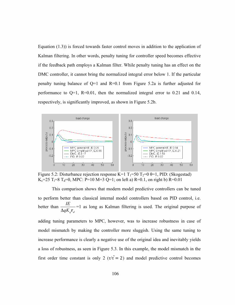
106

Equation (1.3)) is forced towards faster control moves in addition to the application of

Kalman filtering. In other words, penalty tuning for controller speed becomes effective

if the feedback path employs a Kalman filter. While penalty tuning has an effect on the

DMC controller, it cannot bring the normalized integral error below 1. If the particular

penalty tuning balance of Q=1 and R=0.1 from Figure 5.2a is further adjusted for

performance to Q=1, R=0.01, then the normalized integral error to 0.21 and 0.14,

respectively, is significantly improved, as shown in Figure 5.2b.

Figure 5.2: Disturbance rejection response K=1 T1=50 T2=0 θ=1, PID: (Skogestad) Kc=25 Ti=8 Td=0, MPC: P=10 M=3 Q=1; on left a) R=0.1, on right b) R=0.01

This comparison shows that modern model predictive controllers can be tuned

to perform better than classical internal model controllers based on PID control, i.e.

better than q d

IEqK τΔ

=1 as long as Kalman filtering is used. The original purpose of

adding tuning parameters to MPC, however, was to increase robustness in case of

model mismatch by making the controller more sluggish. Using the same tuning to

increase performance is clearly a negative use of the original idea and inevitably yields

a loss of robustness, as seen in Figure 5.3. In this example, the model mismatch in the

first order time constant is only 2 (τ/τ 2) and model predictive control becomes

107

oscillatory. Figure 5.3 depicts the tuning tradeoff between performance and robustness

in model predictive control with a Kalman filter. For the simplified Kalman filter

implementation as described in Chapter 2, the integrated absolute error plot with the

more balanced error and move terms of Q/R=10 (chart a) is notably flatter than that of

the higher performance tuning with Q/R=100 (chart b); this indicates significantly more

robustness to model mismatch in first order time constant. However chart b shows

considerably better control performance around τ/τ 1, i.e. if the model is known

perfectly. What can be observed for general Kalman filter MPC with the same tuning if

τ>τ is the counterintuitive opposite of that of the simplified Kalman filter MPC. As the

move penalties are reduced, the performance becomes better and the curve becomes

flatter. This, however, does not hold true for τ<τ . This effect will be discussed in the

next section, which considers higher order processes.

Figure 5.3: Feedback control performance depending on model mismatch and penalty tuning, K=1 T1=50 T2=0 θ=1, PID: (Skogestad) Kc=25 Ti=8 Td=0, MPC: P=10 M=3 Q=1; on left a) R=0.1, on right b) R=0.01

Bearing the above in mind, it is obvious that MPC penalty tuning is arbitrary

until one considers the impact of model mismatch. . Especially since the setpoint

change performance is not worsened as the disturbance rejection performance is

improved one could tent to unbalance the terms further and further in the direction of

load change response

0

0.2

0.4

0.6

0.8

1

1.2

0 1 2 3

Ta/Tc

IEn general KF

simplified KFSkogestad PID

load change response

0

0.2

0.4

0.6

0.8

1

1.2

0 1 2 3

DTa/DTc

IEn

general KFsimplified KFPID

ˆ/τ τˆ/τ τ

108

the best performance. Chapter 3 discusses methods that automatically determine the

optimal tradeoff based on different robustness and model mismatch criteria.

5.3 Tuning for industrial process characteristics

First order plus deadtime processes are not very representative of processes

controlled by industrial control systems. Common processes in industrial plants include

multiple physical, chemical or biological characteristics that change in series before the

effect on a controlled variable is measured by a sensor. Industrial processes are often

equivalent to a series of dynamic transfer functions. A common control loop includes,

aside from the process, a number of valves, valve positioners and hardware sensors that

may add many additional transfer functions to the loop, thereby potentially increasing

the process model order significantly. Control device and transmitter manufacturers

seek to reduce the impact that time constants of their products have on loop

performance by using fast mechanical linkages and sensor materials. In spite of this, too

much speed and too high sample rates conflict with noise reduction and aliasing

objectives, and may also be very expensive and/or energy consuming. Shinskey points

out the even though industrial processes often have many more time constants, the

resulting overall curve shape can be approximated by a second order process model

with little modeling error because the lags usually interact [8].

109

Figure 5.4: Step response of 20 interacting lags [8]

Figure 5.4 shows the step response of a distillation tower with 20 trays that

effectively creates 20 independent lag time constants in series. The overall curve shape

very closely resembles a second order curve and the resulting time constant may be

calculated by (5.1).

(5.1)

In industrial applications, first and second order approximation of a given

controlled process are most common. Considering a certain amount of model mismatch,

which can never be eliminated, second and third order process models are very

comparable with respect to model error. Thus, industrial users usually model no more

than two time constants, plus deadtime. This section discusses which of the previously

discussed dynamic behaviors are different when controlling a second order plus

deadtime (SOPDT) process. No significant differences could be found when comparing

second to third order plus deadtime processes. Figure 5.5 shows how the tuning

discussed in section 5.3 performs on both a FOPDT and a SOPDT process.

110

Figure 5.5: Feedback control performance depending on model mismatch and penalty tuning, K=1 T1=50 T2=0 θ=1, PID: (Skogestad) Kc=25 Ti=8 Td=0, MPC: P=10 M=3 Q=1; on left a) R=0.1, on right b) R=0.01

As with the FOPDT, the SOPDT also achieves the best possible control

performance at τ=τ (with no model mismatch). However the IAE values are different

since the two different controllers control two different processes: and . Using the algorithm presented in

Chapter 3, the optimal prediction and control horizons are also different between the

two controllers. While P=10 and M=3 is ideal for FOPDT processes, the SOPDT

process is best controlled with P=30 and M=9. This is not surprising, as the additional

order adds another change in slope even though the total settling time of a FOPDT with

50 is very similar to that of a SOPDT with 30 and 20. The two Kalman

filter formulations behave very different if they are connected to a first or second order

process. While MPC with the simplified Kalman filter improves drastically throughout

the entire range and the slope flattens significantly, MPC with general Kalman filter

does considerably worse on the second order process. However, the control

performance of MPC with general Kalman Filter seems to be much less sensitive to

model error. Classical DMC is negatively affected by the introduction of the second

order time constant because its prediction error correction algorithm, biasing the

prediction vector, does not handle model mismatch very well. The presence of a second

load change response

0

0.2

0.4

0.6

0.8

1

1.2

0 1 2 3

DTa/DTc

IEn

general KFsimplified KFPID

load change response

0

0.2

0.4

0.6

0.8

1

1.2

0 1 2 3

Ta/Tc

IEn

general KFsimplified KFPID

ˆ/τ τˆ/τ τ

111

order filter time constant works to the advantage of the model predictive controller with

simplified Kalman filtering. The oscillations that occurred with fast tuning in the

presence of model mismatch (Figure 5.6a) are completely dampened as shown in

Figure 5.6b which plots the same penalty tuning and model mismatch for the MPC

controlling the second order process.

Figure 5.6: Oscillation due to model mismatch (τ/τ =2) on first order (left - a) and second order (right - b) processes, and

. PID: (Skogestad) Kc=25 Ti=8 Td=0, MPC: Q=1 R=0.01; on left a) FOPDT, P=10 M=3 on right b) SOPDT P=30 M=9

As shown in Equation (2.10), simplified Kalman filtering is a state update

method that simplifies tuning by using a tunable filter time constant in the feedback

path. This time constant is set based on knowledge about signal-to-noise ratio.

(2.10)

PID control is also much less sensitive to model mismatch in a second order

process scenario than in a first order process scenario. This is fairly logical because a

PID has two terms that can be used to compensate for two different process time

constants. A PI controller is more suitable for controlling a first order process than

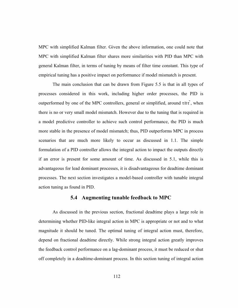
112

MPC with simplified Kalman filter. Given the above information, one could note that

MPC with simplified Kalman filter shares more similarities with PID than MPC with

general Kalman filter, in terms of tuning by means of filter time constant. This type of

empirical tuning has a positive impact on performance if model mismatch is present.

The main conclusion that can be drawn from Figure 5.5 is that in all types of

processes considered in this work, including higher order processes, the PID is

outperformed by one of the MPC controllers, general or simplified, around τ τ , when

there is no or very small model mismatch. However due to the tuning that is required in

a model predictive controller to achieve such control performance, the PID is much

more stable in the presence of model mismatch; thus, PID outperforms MPC in process

scenarios that are much more likely to occur as discussed in 1.1. The simple

formulation of a PID controller allows the integral action to impact the outputs directly

if an error is present for some amount of time. As discussed in 5.1, while this is

advantageous for lead dominant processes, it is disadvantageous for deadtime dominant

processes. The next section investigates a model-based controller with tunable integral

action tuning as found in PID.

5.4 Augmenting tunable feedback to MPC

As discussed in the previous section, fractional deadtime plays a large role in

determining whether PID-like integral action in MPC is appropriate or not and to what

magnitude it should be tuned. The optimal tuning of integral action must, therefore,

depend on fractional deadtime directly. While strong integral action greatly improves

the feedback control performance on a lag-dominant process, it must be reduced or shut

off completely in a deadtime-dominant process. In this section tuning of integral action

113

will be used to fit the MPC controller to the specific fractional deadtime properties of a

process. The integral tuning may even be adapted online automatically if the process

transitions between different regions of fractional deadtime. Such adaptation is practical

because the tuning depends only slightly on model mismatch, as will be shown in this

section. Tuning has much greater dependence on fractional deadtime, which is much

easier to measure than model mismatch.

Since PI and PID are still the most popular feedback controller in the process

control industry, the functionality and tuning of the I-term in a PID controller is well

understood. In some cases, reset and other tuning parameters are calculated based on

known tuning rules [19]. As mentioned before, some tuning rules require a process

model, while others use closed loop characteristics, such as critical gain and critical

period. Even if such parameters are unknown, plant operators and control engineers

often intuitively know how to tune a controller incrementally from the current settings

based on their experience. Figure 5.7 shows how the proportional and integral action of

a PI controller impacts the controller’s load performance for different process

characteristics when an unmeasured unit step disturbance is introduced. Such charts

make it easy to determine whether the ideal setting for a tuning parameter is above or

below the current value. Using the knowledge represented by the charts, it is possible to

find the ideal tuning by trial-and-error without the need to identify a process model.

114

Figure 5.7: Unit step disturbance of PI controllers with different tuning settings. (FOPDT model: K=1, θ=4, τ=20). Ref [72]

Adding integral action (reducing Ti) speeds up the load disturbance rejection but

usually impacts the setpoint change behavior negatively, as previously discussed.

Section 1.4 discusses two degrees of freedom controller formulations that compensate

for this problem, which applies to PID but not model-based control. Such tuning

methods and control equation modifications are clearly not model-based, but empirical.

Whenever researchers or practitioners add tuning parameters to the original three (gain,

reset, rate), it is usually with the intent to better fit the PID algorithm to a particular

usage scenario or group of usage scenarios. Such parameters simplify tuning for the

specific application but often make it harder to tune based on model knowledge.

Som

vs.

com

calc

dist

is n

feed

Fig

the

the

less

metimes the

desired cont

As disc

mponents tha

culation and

turbances wi

not tunable.

dback path o

gure 5.8: Tun

The aug

future error

residuals ar

s impact on

y allow sub

trol perform

cussed in s

at allow dire

d the fact t

ithout any o

Figure 5.8

of a model p

nable integra

gmented inte

r vector (soli

re only one

the control

bstituting of

mance.

ection 5.1,

ect tuning of

that model-b

ffset means

shows how

predictive con

al action in th

egrator can b

id line). The

of the contri

action calcu

115

model know

a model-ba

f the integral

based contr

that they ex

tunable inte

ntroller.

he feedback

be used to in

latter gener

ibuting facto

ulated by the

wledge with

ased contro

action that i

rollers can

xhibit integra

egral action

path of a mo

ntegrate the

rally achieve

ors to the err

e control alg

h knowledge

oller does n

is applied in

account for

al like action

can be augm

odel predicti

residuals (d

es the best re

ror vector, a

gorithm. Fac

about actua

not have an

n the feedbac

r unmeasure

n. However,

mented in th

ive controlle

dotted line) o

esults becaus

and thus hav

ctors that ca

al

ny

ck

ed

it

he

er

or

se

ve

an

116

reduce the impact of a direct integral action which is augmented to residuals are filter

methods for residuals and the setpoint. In both scenarios, the characteristic PID integral

behavior is achieved by adding to the controller output directly, as done in a PID

controller. This allows the controller to react to an unmeasured disturbance more

rapidly and within the same sample period as the disturbance occurred. The huge

benefit of a model predictive controller is that it is able to pre-calculate multiple future

moves based on the process model and future prediction of process outputs.

0

min ( )N k j k j k j

T T Tk j k j k ju j

y Qy u Ru u S u+ + +

∞

+ + +=

+ + Δ Δ∑ (1.3)

When MPC as defined in (1.3) is implemented in a time discrete sampling

control system, it results in a recursive algorithm that uses filter-time constants to

correct for unmeasured disturbances and model mismatch: While the predicted future-

process outputs and target setpoint trajectory are used to calculate the future-control

moves, the predicted future moves are in turn used to update the state variables, i.e., the

future output prediction. A standard MPC as described in (1.3) with default tuning will

correct an unmeasured disturbance as fast as possible in an optimal sense. However, if

there is model mismatch, this recursive calculation will be unbalanced for a longer time

than without model mismatch, which is what the integral term of a PID controller is

designed to pick up and act on. It is therefore possible to distinguish which part of the

future error vector, as shown in Figure 5.8, is a result of setpoint change, versus

unmeasured disturbance. Depending on the tuning of the integral action, the actual

effect of integral tuning will only be noticeable if model mismatch is present. In the

absence of model mismatch, less integral action may be required for the best control

performance. As can be seen in Figure 5.10, for MPC with general Kalman filter the

117

integral action adds very little benefit; at t/t=1 the performance-increasing effect of

integral action becomes more and more obvious as the model mismatch increases. The

resulting control performance charted over time—adding tunable integral action to the

three types of model predictive controller—is depicted in Figure 5.9.

Figure 5.9: Comparison of load rejection performance before and after adding tunable integral action to the future error vector calculation

The PID response is plotted for reference. All three MPCs show a significant

performance improvement. The greatest absolute improvement can be found on the

DMC controller. Its IAE is reduced by 1.49 which is a 47% improvement from the

standard DMC formulation. MPCs with general and with simplified Kalman filter

improve by 29.1% and 46.6%, respectively. The most remarkable finding, however, is

that as the performance improves the robustness does not suffer at all. Figure 5.10

shows a comparison of performance in relation to model mismatch. The MPC plots in

Figure 5.10b not only dropped as compared to Figure 5.10, but also becomes flatter

than, or as flat as, those without augmented integral action.

118

Figure 5.10: Comparison of robustness before and after adding tunable integral action to the future error vector.

The tuning of the integral action is calculated by Skogestad rules, the same way

a PID controller would be tuned, leading to an integral time of Ti=8s. Manual tuning of

the augmented integrator can further improve the feedback control performance. The

empirical tuning described in Figure 5.7 resulted in a stronger integral action with

Ti=4s, shown in Figure 5.11. The integral action can actually be increased even further

until, at Ti=2, the curve slope becomes steeper again, indicating a drip in robustness

without a noticeable gain in performance.

Figure 5.11: Comparison of robustness and performance with manual tuning of integral action on the future error vector

The same tuning analysis was run on the aforementioned second order process

and model predictive controller tuning. As shown in Figure 5.12, the outcome is

surprisingly different. While augmenting an integrator to a FOPDT loop benefitted all

load change response no integral action

0

0.2

0.4

0.6

0.8

1

1.2

0 1 2 3

Ta/Tc

IEn general KF

simplified KFSkogestad PID

load change response, MPC with integral action

0

0.2

0.4

0.6

0.8

1

1.2

0 1 2 3

Ta/Tc

IEn

general KFsimplified KFDMCPID

load change response, MPC with Ti=8s

0

0.2

0.4

0.6

0.8

1

1.2

0 1 2 3

Ta/Tc

IEn

general KFsimplified KFDMCPID

load change response, MPC with Ti=4s

0

0.2

0.4

0.6

0.8

1

1.2

0 1 2 3

Ta/Tc

IEn

general KFsimplified KFDMCSkogestad PIDIMC PIDgeneral KF Ti=4

ˆ/τ τˆ/τ τ

ˆ/τ τˆ/τ τ

119

model predictive controllers, augmenting the exact same integrator to a SOPDT loop

only improved the performance of the MPC with a simplified Kalman filter. As

mentioned above, this type of MPC is relatively insensitive to model mismatch when

applied to a second order process. Thus, lowering the nearly flat performance plot of

the MPC with simplified Kalman filter by such a significant amount results in overlap

with the curve of MPC with general Kalman filter at about τ/τ 2.

Figure 5.12: Comparison of robustness and performance with manual tuning of integral action on the future error vector on second order process

Therefore, we can see that while it is advantageous to use general Kalman

filtering on a second order process, if no or very little model mismatch is expected, one

should switch to simplified Kalman filtering if model mismatch is expected to be

outside of 0.75<τ/τ <2.

If setpoint changes are introduced to a model predictive controller with

augmented integral action, one can observe the same negative effect on setpoint change

performance as seen on PID controllers. Similarity, as with PID control, one can use a

two degrees of freedom formulation to reduce or completely cancel out this effect.

load change response

0

0.2

0.4

0.6

0.8

1

1.2

0 1 2 3

Ta/Tc

IEn

general KFsimplified KFPID

load change response, MPC with integral action

0

0.2

0.4

0.6

0.8

1

1.2

0 1 2 3

Ta/Tc

IEn

general KFsimplified KFPID

ˆ/τ τ ˆ/τ τ

120

5.5 Summary

This chapter showed that the control performance of PID is less impacted by

model mismatch than model-based controllers, such as MPC. Furthermore, the

feedback control performance, i.e. the rejection of unmeasured disturbances, of PID

controllers is better than that of MPC controllers to start with as long as a process is

lagtime-dominant. If the deadtime fraction changes to deadtime-dominant, then MPC is

better at controlling the process because it requires an internal model to account for

deadtime. A method was presented that combines the features of MPC and PID, thereby

positively impacting the feedback control performance. This method takes advantage of

model-based control and integral tuning in the appropriate region of fractional

deadtime. While MPC has inherent integral action that allows offset-free control, the

tuning of integral action is critical to feedback control performance. Conventional PID

tuning rules that favor feedback control performance or adaptive tuning can be applied

to calculate reasonable tuning. Since the integral action is applied to the future error

vector calculation only, it automatically becomes more prominent if the error is caused

by model mismatch (as opposed to disturbance or setpoint change). In other words,

while the integral action contributes when it is needed, it does not diminish

performance when it is not needed. Augmented integral action improves control

performance without reducing robustness.

Another interesting finding was that the impact of integral action drastically

differed if a first or second order process was being controlled. If an algorithm, as the

one presented in Chapter 3 is used to automatically determine all tuning parameters

through optimization, then the model order is an important variable in the objective

121

function. However, significant differences are only observed between first and second

order processes. The difference between second and higher orders is negligible.

While the presented method improves the feedback control performance of

model predictive control significantly, PID still performs better than MPC if model

mismatch is present, i.e. for most of the values for τ/τ 1 in Figure 5.10 to Figure 5.12.

This indicates that there is another feature of PID controllers that is beneficial during

model mismatch and that might be added to augment MPC. Further research could

investigate the benefits and challenges of augmenting derivative action to MPC, in

addition to integral action discussed here.

Based on the newly developed technology suggested in this chapter and the

demonstrated feedback control performance improvements the author is confident that

this method would have had a great positive impact on a challenging process as the one

from Solutia described in the beginning of this chapter. It is conceivable that the MPC

control performance would have been as good or better than the PID control

performance discussed in the beginning of this chapter.

122

Chapter 6

Conclusions and Recommendations

Despite many attempts to broaden the range of applications for model predictive

controllers, their use is still restricted mainly to feedforward, decoupling, constrained

control and optimization applications. One of the reasons for this can be found in the

types of processes than are not controlled well by advanced control strategies such as

MPC. This research focused on identifying these types of processes and analyzing

deficiencies of model predictive controllers for these particular processes. Usually,

when MPC is applied there are high expectations for control performance

improvement. Users of this technology are often unaware of its limitations when

applying it. Since in model predictive control strategies the control performance is

largely dependent on the precision of the plant model, as was shown in Chapter 2,

control performance can degrade very rapidly in some tuning scenarios if model

mismatch is present. Specifically, the feedback control performance is negatively

affected by model mismatch.

The objective of this research was to improve MPC control performance in

scenarios that are currently predominantly solved with PID controllers. The intention

was not to create another PID replacement controller, as has been attempted numerous

times in the past with algorithms like Fuzzy Logic, MPC and others. The intention was

to be able to use the advanced features of MPC in more process scenarios, specifically

feedback control scenarios, where MPC had previously been unable to perform as well

as PID. In other words, the goal of this research was to make MPC applicable to more

types of processes.

123

6.1 Summary of contributions

Chapter 2 analyzed the impact of model mismatch to control performance.

There is abundant literature on state update, and many methods have been developed

that improve the performance of the state update component of a model predictive

controller. The problem of model mismatch is well known in industry and academia.

Since model based controller performance can be severely degraded by model

mismatch, the majority of efforts to improve control performance in model predictive

controllers is focused on improving the performance and precision of state update

algorithms that correct for the effects of model mismatch. Another large portion of

control literature is concerned with improving initial model quality, adapting process

models to process parameter changes, or detecting process parameter changes in order

to inform the user and trigger a manual process model reevaluation. The research

described in this dissertation investigates the direct control performance impact of state

update mechanisms, and shows that optimal control performance can be achieved with

suboptimal state update performance (and vice versa). To date, almost no literature can

be found in this area. Additionally, a very detailed analysis of the impact of controller

tuning in the presence of model mismatch was performed and documented during the

course of research. The tuning relations that are investigated in this work not only

include well known penalty weights, but also some that are not traditionally considered

tuning parameters. Examples include modeling and control horizons, Kalman filter

constants, and types.

Many previously developed solutions that improve MPC control performance in

realistic process scenarios, such as disturbance modeling [20], require knowledge of a

disturbance model and its parameters. Most of such modern methods are derived for

124

perfect models, and lose optimality if model mismatch occurs. Chapter 3 of this

dissertation presented a new automatic method that optimizes control performance for a

given model error by controller tuning, rather than by model improvement or state

update modification. One underlying challenge throughout this research was that no

assumption could be made regarding the process model quality, since in a real plant

there is no such thing as a perfectly known model. This precondition was motivated by

the author’s plant experience during his role in the development of commercial MPC

and control system software. The novel method presented in this work provides optimal

tuning not only for certain fixed amounts of model mismatch, but also for a range of

model mismatch because both the presence and the change in model mismatch (is

usually to be expected. It can do so for any preselected range of ‘worst case’ model

mismatch because an optimization is used to find the best location of an assumed

controller model sub space within the space of optimal tuning values.

Chapter 4 explained the application of this new method and discussed how it

can be used to adapt controller tuning in the following four scenarios (and various

combinations thereof):

1. Manual entry of the actual model, if known

2. Automatic property estimation or model identification based on plant inputs

and outputs

3. Manual entry of model mismatch ranges, if known

4. Automatic estimation of model mismatch based on innovation analysis from

state estimation

Finally, this chapter proposes an adaptive method using existing technology

(autocorrelation of innovation).

125

While the other chapters introduce methods that compensate for known and

unknown model mismatch in an optimal way, the unique contribution of the method

described in Chapter 5 is that the feedback control performance of a model predictive

controller can be improved by a simple addition of tunable integral action. The tuning

of such integral action can be done easily by using the well known and well tested

tuning rules that are used for PI and PID tuning. One big advantage of PID is that it can

be tuned without knowledge of process models. PID tuning methods have been

developed that utilize simple factors to configure desired gain and phase margins [22]

to accommodate a user-specifiable tradeoff between performance and robustness. Many

tuning methods allow testing the process with very little perturbation [23]. At the same

time, the abundance of tuning rules can be a disadvantage [19]. Chapter 5 proposed a

novel method to improve model predictive control performance by augmenting tunable

integral action. The contribution to the field is a method that uniquely utilizes

knowledge of the dynamic behavior of disturbances to calculate corrective action that

can be added directly to the manipulated variable of a model predictive controller. This

is similar to how a PID algorithm includes past error characteristics in the calculation of

corrective action and improves the feedback control performance dramatically for

control scenarios with model mismatch and/or changing dynamics. No such algorithm

is used in today’s MPC controllers. Future research may investigate stability margins

and an automatic method to find the optimal tuning parameters. The impact of

augmenting derivative action might also be investigated in future research.

126

6.2 Recommendations for future research

There are several courses that future research might take, such as investigating

more criteria, like the effect of deadtime, and more complex process models or

multivariable processes. These further degrees of freedom were consciously omitted in

this work, however, for logical or scope reasons. The intention of this research was to

present new concepts for improving control performance in the presence of model

mismatch. These concepts were tested in simulation and in plant experiments that

involved an actual digital control system which was connected to real plant equipment

and running a chemical process. Further research might also investigate more additional

criteria, such as additional tuning parameters, higher order models, or more customized

definitions of control performance and stability.

Additionally, selected parts of this research could be extended to multivariable

scenarios, as large process handling and optimization are two of the key selling features

that MPC has over other control strategies, such as PID.

The conceptual design of a fully automatic adaptive controller that uses the

optimal MPC tuning method that has been presented in Chapter 4 is far from being

complete. Further research in this area should investigate how multiple alternate tuning

scenarios can be implemented in an automatic fashion with minimal impact to plant

operation, and without affecting the autocorrelation method itself or creating positive

feedback. Further research in this area could investigate the ideal model update trigger

functions or even gain scheduling methods. Before commercial usage or productization

of such automatic method is feasible, more sophisticated safety nets have to be

developed. A wider variety of process and model types may be researched in future

127

research. Also work could be done to quantify and normalize the amount of model

mismatch as an easy to understand generic metric.

Just as Chapter 5 discussed how the feature of tunable integral action can

improve MPC control performance, future research could investigate the use of tunable

derivative action. Derivative tuning is a well known and understood feature in the user

community that is often used to overcome the effects of unknown nonlinearities and has

potential to benefit modern advanced control strategies such as MPC.

128

Bibliography

[1] C. R. Cutler and B. L. Ramaker, Dynamic matrix control – a computer control algorithm, Proc. Automatic Control Conf. Paper WP5-B, San Francisco, CA, 1980

[2] R. E. Otto, Forward modeling controllers: a comprehensive SISO controller, AIChe meeting, November 5, 1986

[3] G. Pannocchia, N. Laachi, J. B. Rawlings, A candidate to replace PID Control: SISO Constraint LQ Control, DYCOPS Proceedings, (2004)

[4] ADCO – adaptive Riccati controller, 1992, http://www.ipas-systeme.de/products111.htm

[5] A. Hugo, Limitations of model predictive controllers, Hydrocarbon Processing, Jan 2000, pp 83-88

[6] M. Jelali. An overview of control performance assessment technology and industrial applications. Control Engineering Practice, 14:441–466, 2006.

[7] T. Olsen, B. Bialkowski, EnTech Control, Session No. 42 - Applications of Control to Refining, AIChE Spring National Meeting in New Orleans, March 2002

[8] G. Shinskey, Process Control: As Taught vs. as Practiced, Ind. Eng. Chem. Res. 41, 3745-3750, 2002

[9] S. Skogestad, Simple analyticRules for Model Reduction and PID Controller Tuning, J. Process Control 13, 291, 2003

[10] K. Aström, T. Hӓgglund, PID Controllers Theory, Design and Tuning, 2nd ed., ISA, Research Triangle Park, NC, 1995

[11] T. L. Blevins, G. K. McMillan, W. K. Wojsznis and M. W. Brown, Advanced Control Unleashed, ISA, 2003, ISBN 1-55617-815-8

[12] A. S. Morse, F. M. Pait, S. R. Weller, “Logic-Based Switching Strategies for Self-Adjusting Control,” 33rd IEEE Conference on Decision and Control, Workshop Number 5. Lake Buena Vista, Florida, USA, December 1994.

[13] K. S. Narendra, and J. Balakrishnan, “Adaptive Control Using Multiple Models,” IEEE Transactions on Automatic Control,. Vol. 42, No. 2, pp.177-187, February 1997.

129

[14] G. K. McMillan, Good Tuning: a Pocket Guide, 2nd edition, ISA, 2005, ISBN 1-55617-940-5

[15] D. Thiele, T. L. Blevins, W. K. Wojsznis, Autotuning In Distributed Environment, ISA1999, Philadelphia

[16] D. Thiele, W. K. Wojsznis, A. Mehta, Achieving nonlinear MPC performance with neural network aided state update, ISA 2004, Houston

[17] D. Thiele, Benefits and challenges of implementing model predictive control as a function block, ISA2000, New Orleans

[18] Integrated model predictive control and optimization within a process control system, US Pat. 7050863 - Filed Jul 25, 2003 - Fisher-Rosemount Systems, Inc.

[19] A. O’Dwyer, PI and PID controller tuning rules for time delay processes: a summary. Dublin Institute of Technology, Dublin, Ireland, 15 May 2000

[20] T. Badgwell, K. Muske, Disturbance Model Design for linear Models. Proceedings of ACC, 1621-1626, Anchorage, AK, May 2002

[21] P. Lundstrom, J. Lee, M. Morari, S. Skogestad, Limitations of dynamic matrix control. Computers in Chemical Engineering 19, 409-421, 1995

[22] W. Wojsznis, J. Gudaz, T. Blevins and A. Mehta, Practical approach to tuning MPC, ISA transactions (ISA trans.), 42(1), 149–162, 2003

[23] W. Wojsznis, T. Blevins: „Systems and Method for automatically tuning a Process Controller”, US Patend Number 5,453,925, September 1995

[24] G. Shinskey, Feedback Controllers for the Process Industries, McGraw Hill, 1994

[25] G. Shinskey, PID-deadtime control of distributed processes, 2001

[26] R.E. Kalman, A new approach to linear filtering and prediction problems, Journal of Basic Engineering 82 (1): 35–45, 1960

[27] M. Morari, N. L. Ricker, Model Predictive Control Toolbox User’s Guide, 1998

[28] G. McMillan, Implementing MPC to Reduce Variability by Optimizing Control Valve Response, 2005

[29] R. Cagienard, P. Grieder, E. Kerrigany and M. Morari, Move Blocking Strategies in Receding Horizon Control, 43rd IEEE CDC, 14-17 Dec. 2004, Page(s): 2023 - 2028 Vol.2

[30] Y. Takahashi, M. J. Rabins, D. M. Auslander, Control and Dynamic Systems, Addison-Wesley, Reading, Massachusetts (1972)

130

[31] J. H. Lee, M. Morari and C. E. Garcia, State Space interpretation of model predictive control, Automatica, Vol 30, No. 4, pp. 707-717 (1994)

[32] S. Qin, T. Badgwell, A Survey of Industrial Model Predictive Control Technology, Control Engineering Practice, Volume 11, Issue 7, July 2003, Pages 733-764

[33] Bo Han; Xinggang Lin, Adapt the steady-state Kalman gain using the normalized autocorrelation of innovations, Signal Processing Letters, IEEE, Volume 12, Issue 11, Nov. 2005 Page(s): 780 – 783

[34] J. Maršik and V. Strejc, Application of Identification-free Algorithms for Adaptive Control, Automatica, Vol. 25, No. 2, pp.273--277, 1989.

[35] J. Maršik, P. Jaroslav, A nonlinear adaptive PID controller, IFIP Conference on Optimized-Based Computer-Aided Modeling and Design, Prague, Czech Republic, May, 1994.

[36] D. Thiele, W. Wojsznis, Multi Model Adaptive Industrial MPC Controller, Proceedings Control and Applications, Montreal, Canada, 2007

[37] W. Wojsznis, T. Blevins, Evaluating PID adaptive techniques for industrial implementation, Proceedings of the American Control Conference 2002, Page(s): 1151 - 1155 Volume 2

[38] P. Kesavan and J. H. Lee, A set based approach to detection and isolation of faults in multivariable systems, Elsevier Science Ireland, 2001

[39] B. J. Odelsen & Rawlings, Estimating Disturbance Covariances From Data For Improved Control Performance, Dissertation University of Wisconsin - Madison, 2003

[40] F. G. Shinskey, PID-deadtime control of distributed processes, Control Engineering Practice, Volume 9, Number 11, November 2001 , pp. 1177-1183(7), 2001

[41] G. Pannocchia, N. Laachi, and J. B. Rawlings. A candidate to replace PID control: SISO constrained LQ control. AIChE J., 51(4):1171-1189, 2005

[42] T. Hӓgglund, K. Aström, Method and an apparatus in tuning a PID-regulator - US Patent 4,549,123, 1985

[43] DeltaV, digital Process automation system, www.EasyDeltaV.com

[44] G. Pannocchia, G. and E. C. Kerrigan, Offset-free Control of Constrained Linear Discrete-time Systems Subject to Persistent unmeasured disturbances, In 42nd IEEE conference on decision and control, Hawaii, USA (2003)

[45] W. K. Wojsznis, T. L. Blevins, D. Thiele, Neural Network Assisted Control Loop Tuner, 2005, patent number 6847954

131

[46] CJCSim; http://www.cutlerjohnston.com/products.htm

[47] http://www.aspentec.com/includes/product.cfm?IndustryID=0&ProductID=54

[48] http://www.hyprotech.com/products/family.asp?ID=1

[49] A. Badwe, R. Patwardhan, S. Patwardhan, R. Gudi, Quantifying the Impact of Model-Plant Mismatch on Controller Performance: A non-invasive approach, International Symposium on Advanced Control of Industrial Processes (ADCONIP 2008)

[50] C. Desoer, M. Vidiyasagar, Feedback Systems: Input-output properties, Academic Press, New York, 1975

[51] N. Stanfelj, T. Marlin, J. MacGregor, Monitoring and Diagnosis of Process Control Performance: The Single Loop Case, Ind. Eng. Chem. Res., 32, 301-314, 1993

[52] P. Kesevan and J.H. Lee. Diagnostic tools for multivariable model-based control systems. Ind. Eng. Chem. Res., 36(7):2725–2738, 1997

[53] B. J. Odelson and J.B. Rawlings. Online monitoring of MPC disturbance models using closed-loop data. In Proceedings of the American Control Conference, pages 2714–2719, Denver, CO, 2003.

[54] J. M. Maciejowski, Predictive Control with Constraints, Prentice Hall, 2002, Shell oil fractionator, p 248

[55] OPC Foundation: http://www.opcfoundation.org

[56] DeltaV Tune: http://www.easydeltav.com/pd/PDS_DeltaV_Tune.pdf

[57] Emerson Process Management, DeltaV Documentation

[58] Kenneth R. Muske and James B. Rawlings. Model predictive control with linear models. AIChE J., 39(2):262-287, 1993.

[59] J. Richalet, A. Rault, J. L. Testud, and J. Papon. Model predictive heuristic control: Applications to industrial processes. Automatica, 14:413-428, 1978.

[60] C. R. Cutler and B. L. Ramaker. Dynamic matrix control|a computer control algorithm. In Proceedings of the Joint Automatic Control Conference, 1980.

[61] D. M. Prett and R. D. Gillette. Optimization and constrained multivariable control of a catalytic cracking unit. In Proceedings of the Joint Automatic Control Conference, 1980.

[62] C. E. Garcia and A. M. Morshedi. Quadratic programming solution of dynamic matrix control (QDMC). Chem. Eng. Commun., 46:73-87, 1986.

132

[63] P. Grosdidier, B. Froisy, and M. Hammann. The IDCOM-M controller. In T. J. McAvoy, Y. Arkun, and E. Zafiriou, editors, Proceedings of the 1988 IFAC Workshop on Model-based Process Control, pages 31-36, Oxford, 1988. Pergamon Press.

[64] P. Marquis and J. P. Broustail. SMOC, a bridge between state space and model predictive controllers: Application to the automation of a hydrotreating unit. In T. J. McAvoy, Y. Arkun, and E. Zafiriou, editors, Proceedings of the 1988 IFAC Workshop on Model-based Process Control, pages 37-43, Oxford, 1988. Pergamon Press.

[65] R. Shridar, D. Cooper, A tuning strategy for unconstrained multivariable model predictive control, Ind. Eng. Chem. Res., 37(10), 4003–4016, 1998

[66] J. Trierweiler, L. Farinab, RPN tuning strategy for model predictive control, J. of Process Control, 13(7), 591–598, 2003

[67] J. Garriga, M. Soroush, Eigenvalue Pole Placement Using Model Predictive Control, 2007

[68] S. Patwardhan, S. Shah, From data to diagnosis and control using generalized orthonormal basis filters. Part I: Development of state observers, J Process Control 15, 2005

[69] T. S. Schei, On-line Estimation of process control and Optimization Applications, 8th International IFAC Symposium on Dynamics and Control of Process Systems, Preprints Vol. 2, June 6-8, Cancún, Mexico

[70] B. Han, X. Lin, Adapt the Steady-State Kalman Gain Using the Normalized Autocorrelation of Innovations, IEEE Signal Processing Letters, Vol. 12, No. 11, November 2005

[71] S. Ko, R. R. Bitmead, State Estimation of Linear Systems with State Equality Constraints, IFAC 2005

[72] D. E. Seborg, T.F. Edgar, and D.A. Mellichamp, Process Dynamics and Control 2nd Ed.,New York: Wiley, 2004

133

Vita