13

THIELE CENTREfor applied mathematics in natural science

THIELE CENTREfor applied mathematics in natural science

On the Laplace transformof the Lognormal distribution

Søren Asmussen, Jens Ledet Jensenand Leonardo Rojas-Nandayapa

www.thiele.au.dk

The T.N. Thiele CentreDepartment of Mathematical SciencesUniversity of Aarhus

Ny Munkegade 118, Bldg. 15308000 Aarhus CDenmark

Phone +45 89 42 35 15Fax +45 86 13 17 69Email thiele@imf.au.dk Research Report No. 06 November 2013

On the Laplace transform of the Lognormaldistribution

Søren Asmussen1, Jens Ledet Jensen1 and Leonardo Rojas-Nandayapa2

1Department of Mathematics, Aarhus University2School of Mathematics and Physics, University of Queensland

AbstractIntegral transforms of the lognormal distribution are of great importance instatistics and probability, yet closed-form expressions do not exist. A widevariety of methods have been employed to provide approximations, both ana-lytical and numerical. In this paper, we analyze a closed-form approximationL(θ) of the Laplace transform L(θ) which is obtained via a modified versionof Laplace’s method. This approximation, given in terms of the Lambert W (·)function, is tractable enough for applications. We prove that L(θ) is asymptot-ically equivalent to L(θ) as θ →∞. We apply this result to construct a reliableMonte Carlo estimator of L(θ) and prove it to be logarithmically efficient inthe rare event sense as θ →∞.

Keywords: Lognormal distribution, Laplace transform, Characteristic func-tion, Moment generating function, Laplace’s method, Saddlepoint method,Lambert W function, rare event simulation, Monte Carlo method, Efficiency.

MSC: 60E05, 60E10, 90-04

1 Introduction

The lognormal distribution is of major importance in probability and statistics asit arises naturally in a wide variety of applications. For instance, the central limittheorem implies that the limit distribution of a product of random variables often canbe well approximated by the lognormal distribution. Hence it is not surprising thatthe lognormal distribution is frequently employed in disciplines such as engineering,economics, insurance or finance, and it often appears in modeling across the sciencesincluding chemistry, physics, biology, physiology, ecology, environmental sciences andgeology; even social sciences and linguistics, see [1–5].

The lognormal distribution Fµ,σ2 is defined as the distribution of the exponentialof a N(µ, σ2) random variable and has density

f(x) =1

x√

2πσexp

{−(log x− µ)2

2σ2

}, x ∈ R+.

Corresponding author: Leonardo Rojas-Nandayapa, l.rojas@uq.edu.au

1

However, closed-form expressions for transforms of the lognormal distribution do notexist and reliable numerical approximations are scarce. In particular, an inspectionof the defining integrals

L( θ) =

∫ ∞

0

e−θxdFµ,σ2(x) =

∫ ∞

0

1

x√

2πσexp

{−θx− (log x− µ)2

2σ2

}dx,

=

∫ ∞

−∞

1√2πσ

exp

{−θet − (t− µ)2

2σ2

}dt (1.1)

for the Laplace transform L( θ) reveals that there is very little hope in findinga closed form expression for transforms of the lognormal distribution (note thatthe Laplace transform and the characteristic function ϕ are connected by ϕ(ω) =L(−iω), L(θ) = ϕ(iθ)). Moreover, the integral defining L( θ) diverges when <(θ) < 0and in consequence, the function L( θ) is not defined in the left half of the complexplane and fails to be analytic on the imaginary axis (thus, the moment generatingfunction is not defined). Nevertheless, in the absence of a closed-form expressionit is desirable to have sharp approximations for the transforms of the lognormaldistributions as this paves the road for obtaining the distribution of a sum of i.i.d.lognormal random variables via transform inversion.

In this paper, we further analyze the closed form approximation of the Laplacetransform of the Lognormal distribution which we reported in [6] and was obtainedvia a modified version of Laplace’s method. Such expression will be denoted L(θ)and it is given by

L(θ) =

exp

{−W 2(θeµσ2) + 2W (θeµσ2)

2σ2

}

√1 + W (θeµσ2)

, θ ∈ R+. (1.2)

In the expression above, W ( · ) is the Lambert W function which is defined as thesolution of the equation W (x)eW (x) = x; this function has been widely studied inthe last 20 years mainly due to the advent of fast computational methods, cf. [7].Roughly speaking, the standard Laplace’s method [8] states that an integral of thegeneral form

∫ b

a

e−θh(t) g(t) dt =

√2π e−θh(ρ)√θh′′(ρ)

g(ρ)(1 + O(θ−1)

), θ →∞, (1.3)

where g(t) and h(t) are functions such that g(t) is “well behaved” and h(t) has aunique global minimum at ρ ∈ (a, b). Therefore, the leading term of the expressionon the right hand side of (1.3) can be used as an asymptotic approximation of theintegral on the left hand side. Surprisingly, this approximation can be very accuratefor very general functions g(t) and h(t), not only in asymptotic regions but also forrelatively small values of θ. In our case, we employ a variant of Laplace’s methodby first noting the following

Lemma 1.1. Let θ > 0. Then the exponent hθ(t) := −θet − (t − µ)2/2σ2 in theintegrand in (1.1) has a unique maximum at ρθ = −W (θeµσ2) + µ.

2

We then proceed in similar way as in the standard Laplace’s method with g(t) ≡ 1and h(t) = −hθ(t)/θ dependent on θ. However, we also pay a price for such mod-ification: the expression derived is no longer of an asymptotic order 1 + O(θ−1) asgiven in formula (1.3). In the following section we will prove that

L(θ) = L(θ)(1 + O(log−1(θ))), θ →∞,

so the modification increases the order of the asymptotic series. Yet, the suggestedapproximation remains asymptotically equivalent to the true Laplace transform asthe value of the argument goes to infinity. Moreover, based on these results wewill obtain a probabilistic representation of the error term and construct a MonteCarlo estimator for the Laplace transform. We remark that one must be carefulin the implementation of Monte Carlo estimators as naive simulation can lead tounreliable approximations. We show that our proposal corresponds to an importancesampling estimator which delivers reliable estimates for any value of the argumentby proving its asymptotic efficiency in a rare-event sense to be defined. We furtherprovide numerical comparisons of our proposal against other methods available inthe literature.

We note that the problem of approximating the transforms of a lognormal isof high complexity and it has been long standing. Therefore, a significant numberof methods have been developed to approximate both the Laplace and the charac-teristic functions of the lognormal distribution. We give a more complete literaturesurvey at the end in Section 5 and mention here the work which is most relevant forthe present paper. Barakat [9] introduced the term iω(−t−1) in the exponent of theintegrand defining the characteristic function and by taking a series representationof eiω(e

t−t−1), he obtains a representation in terms of Hermite polynomials after inte-grating term by term. Holgate [10] employed the classical saddle point method [11],which consists in applying Cauchy’s theorem to deform the path of integration insuch a way that it traverses through a saddlepoint of the integrand in the steepestdescent direction. In the lognormal case, the saddlepoint is given as the solutiont = ρ(ω) of the equation te−t = iσ2ω, so the saddlepoint approximation of thecharacteristic function is of the form

ϕ(ω) ∼ (1− ρ(ω))−1/2 exp{(ρ(ω)2 − 2ρ(ω)

)/2σ2

}. (1.4)

Gubner [12] employed (as many others) numerical integration techniques and wasthe first in proposing alternative path contours to reduce the oscillatory behaviorof the integrand. This approach was further extended in Tellambura and Senaratne[13] where they proposed specific contours passing through the saddlepoint at asteepest descent rate; this election has the effect that oscillations are removed in aneighborhood around the saddlepoint. In addition, they also addressed the heavy-tailed nature of the lognormal density by proposing a transformation which deliversan integrand with lighter tails.

In this paper we followed a path somewhat different from Holgate to approximatethe Laplace transform of a Lognormal distribution (1.1) by using a variant of theLaplace’s method (related to the saddlepoint method). To the best of our knowledge,the resulting closed form approximation (1.2) derived from this methodology wasfirst reported in [6].

3

The paper is organized as follows: In Section 2 we compute the approximation ofthe Laplace transform of the lognormal distribution and analyze its asymptotic prop-erties; in addition, we extend this result to the complex plane via the saddlepointmethod and establish the relationships with the results of Holgate. In section 3 weconstruct an importance sampling estimator for approximating the Laplace trans-form and prove its efficiency properties; we discuss the disadvantages of using naïveMonte Carlo for estimating this Laplace transform. We verify the sharpness of ourapproximations and present some numerical comparisons in the analysis presentedin Section 4. A discussion and concluding remarks are in Section 5.

2 Approximating the lognormal Laplace transform

We start by proving Lemma 1.1.

Proof of Lemma 1.1. Recall that for z ∈ (−e−1,∞) the Lambert W function w =W (z) is defined as the unique solution w ∈ (−1,∞) of the equation wew = z. Withthe change of variables t = µ− y we have hθ(y) = −θeµe−y − y2/2σ2,

h′θ(y) = θeµe−y − y

σ2=

e−y

σ2

(θeµσ2 − yey

).

Here θeµσ2 − yey is equal to 0 for y = W (θeµσ2), positive for 0 ≤ y < W (θeµσ2),and negative for W (θeµσ2) < y <∞ since yey is strictly increasing on [0,∞). Alsoθeµσ2 − yey > 0 for y < 0 since then yey > 0. This shows that there is a uniquemaximum at y = W (θeµσ2), i.e. at t = µ−W (θeµσ2).

In the rest of this section we will make the approximation (1.2) more precise.In Proposition 2.1, we show that L(θ)/L(θ) is given in terms of a certain expectedvalue, which in Proposition 2.2 we show goes to 1 as θ →∞. Finally, we note thatthe approximation derived from Proposition 2.1 can be embedded in a more generalresult which is valid in the right half of the complex plane including the imaginaryaxis (Remark 2.7).

We assume that µ = 0. Notice that such assumption is made without loss ofgenerality as Lµ,σ2(θ) = L0,σ2(e−µθ) where Lµ,σ2 stands for the Laplace transform ofa lognormal random variable with parameters µ and σ2 (we also drop the subindexesµ and σ2 used in the notation above and adopt the notation L(θ) for the rest of thepaper).

The approximation L(θ) given in (1.2) is derived from the following proposition:

Proposition 2.1. The Laplace transform of F0,σ2 can be written as

L(θ) =

exp

{−W 2(θσ2) + 2W (θσ2)

2σ2

}

√1 + W (θσ2)

E[g(σ(θ)Z; θ

)], θ > 0. (2.1)

where Z is an independent normal standard random variable, σ2(θ) = σ2/

(1 +W (θσ2)) and

g(t; θ)

= exp

{−W (θσ2)

σ2

(et − 1− t− t2

2

)}, t ∈ R.

4

Observe that equality (2.1) in the previous proposition expresses the Laplacetransform of a lognormal distribution as the product of two terms: 1) a closed-formexpression in terms of the function Lambert W (·) and 2) an expected value of atransformed standard normal random variable Z.

The first corresponds to the closed from approximation L(θ) given in (1.2) andobtained by the modified version of the Laplace’s method. The heuristic argumentsused for its construction are illustrated next. Consider the representation

L(θ) = E[e−θX ] =

∞∫

−∞

1

σ√

2πexp{−θet − t2

2σ2

}dt, θ > 0, (2.2)

and the infinite series representation of hθ(t) = −θet − t2/2σ2 around its maximumρθ = −W (θσ2) (recall Lemma 1.1). By truncating the series up to terms of secondorder we can obtain a good approximation of the integral because the exponentialtransformation makes the contribution from regions away from ρθ small. Therefore,most of the total value of the integral will come from a region around the modepoint ρθ where the two functions have similar values. This truncated integral can besolved explicitly and its value corresponds to the first term in (2.1).

The correction term derived from the use of the Laplace’s method comes inthe form of an expected value so it provides a probabilistic representation of theerror associated to such approximation. A crucial advantage of this representationis that this approximation can be sharpened via a careful implementation of theMonte Carlo method (section 3). Observe that the function g( · ; θ) roughly equals1 in a neighborhood of 0; in consequence, the value E

[g(σ(θ)Z; θ

)]is relatively

close to 1. In fact, we will prove that the modified Laplace’s method delivers anapproximation with an error which is asymptotically negligible. Moreover, it turnsout that this approximation is sharp all over the domain of convergence of θ as wewill empirically corroborate in the numerical examples in section 4.

The proof of Proposition 2.1 provides transparency to the heuristic argumentsof the modified version of the Laplace’s method discussed above.

Proof of Proposition 2.1. Consider the expression (2.2) for the Laplace transform.Lemma 1.1 implies that the maximum of the integrand occurs at ρθ = −W (θσ2). Toimplement the Laplace’s method we consider a second order approximation of theexponent around the mode point that is introduced in the exponent of the integrand;then using the identity −θe−W (θσ2) = −W (θσ2)/σ2 we rewrite the r.h.s. of (2.2) as

1√2πσ

∞∫

−∞

exp

{− W (θσ2)

σ2

[1 + (t+ W (θσ2))

+(t+ W (θσ2))2

2

]− t2

2σ2

}g(t+ W (θσ2); θ

)dt (2.3)

where the function g collects all the remaining terms, i.e.

g(t; θ) = exp

{−W (θσ2)

σ2

(et − 1− t− t2

2

)}.

5

After some extensive, but otherwise standard algebraic manipulations involving thefunction W (·) and its properties, expression (2.3) becomes

exp

{−W (θσ2)2 + 2W (θσ2)

2σ2

}

√1 + W (θσ2)

·∞∫

−∞

1√2πσ(θ)

exp

{−(t+ W (θσ2))2

2σ2(θ)

}g(t+ W (θσ2); θ

)dt,

where σ(θ)2 = σ2/(1 + W (θσ2)). The result of the proposition follows with a changeof variable y = (t+ W (θσ2))/σ(θ).

We refer to L(θ) in (1.2) as the LM-approximation of the Laplace transform of thelognormal distribution (this name will be frequently used in our numerical investiga-tions in Section 4). In the following proposition we make use of the asymptotic rep-resentation of the standard Laplace’s method to prove that the LM-approximationis asymptotically equivalent to the true Laplace transform and demonstrate thatthe relative error of the approximation of L(θ) vanishes at a rate of convergence oforder log(θ)−1.

Proposition 2.2. E[g(σ(θ)Z; θ

)] = 1 + O

(log(θ)−1

)as θ →∞.

Corollary 2.3. L(θ) = L(θ)(1 + O(log(θ)−1)),

limθ→∞

L(θ)

L(θ)= 1, lim

θ→∞L(θ) = lim

θ→∞L(θ) = 0.

[For the last assertion, just note the obvious fact that the L(θ) → 0 as θ → ∞]. Itis also appealing to summarize the asymptotic behavior of L(θ) in the rough formof logarithmic asymptotics familiar from large deviations theory:

Lemma 2.4.limθ→∞

W (θ)

log(θ)= 1, lim

θ→∞

logL(θ)

log2 θ= − 1

2σ2.

[For the first assertion, just use L’Hopital and W ′(θ) = W (θ)/(θW (θ) + θ)].The proof of Proposition 2.2 is given in two parts. First we prove that the integral

over an open interval containing the mode point is asymptotically equal to 1. Thisis accomplished by employing a standard asymptotic result which also providesinformation about the asymptotic order of convergence. The second part of theproof consists in proving that the contribution to the integral coming from the tailsis negligible as the value of the argument θ →∞. Consequently, we conclude that theexpected value goes to 1 as the value of the argument goes to infinity. In addition, wewill require both the asymptotic result in the first part of Lemma 2.4 and Lemma 2.5below, which provides an alternative representation of the expected value in (2.1) ina form that will useful to construct upper bounds satisfying the required asymptoticconditions. Moreover, Lemma 2.5 will be use later for the construction of efficientMonte Carlo estimators of the Laplace transform.

6

Lemma 2.5. Let g(·; θ), σ2(θ) and Z be defined as in Proposition 2.1. Then

E[g(σ(θ)Z; θ

)]=√

1 + W (θσ2)E[ϑ(σZ; θ)] (2.4)

whereϑ(t; θ) = exp

{−W (θσ2)

σ2

(et − 1− t

)}, t ∈ R.

Furthermore, E[g(σ(θ)Z; θ

)]≤√

1 + W (θσ2) for all θ > 0.

Proof of Lemma 2.5.

E[g(σ(θ)Z; θ)] =

∫ ∞

−∞exp

{−W (θσ2)

σ2

(eσ(θ)t − 1− σ(θ)t− σ2(θ) t2

2

)− t2

2

}dt

=

∫ ∞

−∞ϑ(σ(θ) t; θ) exp

{−t

2

2

(− W (θσ2) σ2(θ)

σ2+ 1

)}dt

=

∫ ∞

−∞ϑ(σ(θ) t; θ) exp

{−1

2· t2

1 + W (θσ2)

}dt.

The change of variable z = t/√

1 + W (θσ2) yields E[g(σ(θ)Z; θ

)]=√

1 + W (θσ2)·E[ϑ(σZ; θ)]. The upper bound follows from the observation that ϑ(t; θ) ≤ 1 for allt ∈ R and θ > 0. This completes the proof of the Lemma.

Proof of Proposition 2.2. Consider the representation (2.4) in Lemma 2.5 and rewrite

E[ϑ(σZ; θ)] =

∫ a

−∞ϑ(σt; θ)φ(t)dt,+

∫ b

a

ϑ(σt; θ)φ(t)dt,+

∫ ∞

b

ϑ(σt; θ)φ(t)dt, (2.5)

where φ(t) is the density of the standard normal distribution; a, b are selected suchthat 0 ∈ (a, b). For the second integral we can apply a standard asymptotic resultfor the standard Laplace’s method [cf. p. 44, 14], which says that if a function h(z)has a single minimum (mode point) z ∈ (a, b) then it holds that

∫ b

a

e−ηh(z)φ(t)dt =

√2πe−ηh(z)√η h′′(z)

φ(z)(1 + O(η−1)

), η →∞,

In our specific case, η = W (θσ2), and z = 0 is the mode point of the functionh(t) = (eσt − 1 − σt)/σ2. Since h(0) = 0, h′′(0) = 1 and φ(0) = (2π)−1, then itfollows that

∫ b

a

ϑ(σt; θ)φ(t) dt =1√

W (θσ2)

(1 + O(W (θ)−1)

), θ →∞. (2.6)

For the first integral we use ϑ(σt; θ) ≤ exp{−W (θσ2)σ−2(−1 − σt)} to obtain anupper bound:

∫ a

−∞ϑ(σt; θ)φ(z) dt ≤

∫ a

−∞exp

{−W (θσ2)

σ2

(− 1− σt

)}φ(t)dt

= exp

{W 2(θσ2) + 2W (θσ2)

2σ2

}Φ

(aσ −W (θσ2)

σ

)

7

where Φ(·) corresponds to the normal standard distribution. Using Mill’s ratio wefind that the previous expression is asymptotically equivalent to

exp

{W 2(θσ2) + 2W (θσ2)

2σ2

}σ√

2π∣∣aσ −W (θσ2)

∣∣ exp

{−(aσ −W (θσ2))2

2σ2

}

∼ exp

{(1 + aσ)W (θσ2)

σ2− a2

2

}σ√

2πW (θσ2)(2.7)

For the third integral we have that ϑ(σt; θ) < exp{−W (θσ2) t2/2σ2} for t ≥ 0. Then∫ ∞

b

ϑ(σt; θ) dΦ(t) <

∫ ∞

b

exp

{−W (θσ2)t2

2σ2

}dΦ(t)

=

∞∫

b

1√2π

exp

{−(1 + W (θσ2)σ−2)t2

2

}dt

= 1− Φ(b√

1 + W (θσ2)σ−2)

(2.8)

Using Mill’s ratio we obtain the following asymptotically equivalent expression

1

b√

2π(1 + W (θσ2)σ−2)exp

{−b

2(1 + W (θσ2)σ−2)

2

}.

Now, observe that if we select a < −σ−1, then the asymptotic order of the tailintegrals (2.7)-(2.8) is negligible compared to the asymptotic order of the integralin the interval (a, b) given in expression (2.6). Hence, using Lemma 2.5 and theasymptotic equivalence (2.6) we obtain

E[g(σ(θ)Z; θ

)]=√

1 + W (θσ2)

∫ ∞

−∞ϑ(σt; θ) dΦ(t)

=√

W (θσ2)−1 + 1 ·(1 + O(W (θσ2)−1)

). (2.9)

Since√

W (θσ2)−1 + 1 = 1 + O(W (θσ2)−1) if follows that E[g(σ(θ)Z; θ

)]= 1 +

O(W (θσ2)−1). Using the first part of Lemma 2.4 we obtain that W (θσ2) ∼ log(θ)as θ →∞. This completes the proof.

The term O(log(θ)−1) in Proposition 2.2 arising from the approximation ofLaplace’s method can be further expanded into an asymptotic series, so we canobtain more information on the asymptotic behavior of the Laplace transform ofthe Lognormal distribution. For instance, the statement in Remark 2.6 provides asecond order term from the asymptotic series. Its proof is similar to that of Propo-sition 2.2.

Remark 2.6.

E[g(σ(θ)Z; θ

)] = 1 +

σ2

12 log(θ)+ O

(log(θ)−2

).

8

However, one must be careful when using asymptotic series as approximations ofthe real Laplace transform because it is common to obtain asymptotic series whichare divergent for certain given values. For instance, the second term in the asymptoticseries obtained above σ2/12 log(θ) → ∞ as θ → 0. One could employ asymptotictechniques to obtain an optimal approximation by truncating the asymptotic seriesup to a certain term. However, in our numerical results we found that the numericalapproximation derived from this strategy delivered poor numerical results even inregions away from θ = 0. An alternative delivering better numerical results is theMonte Carlo method which we explore in the section 3.

Proof of Remark 2.6. Take the function h(z) = (eσz−1−σz)/σ2, which has a modepoint at z = 0. Then, the term O(W (θσ2)−1) in the decomposition (2.9) has thefollowing expansion [cf. 2.20, 14]

1

W (θσ2)

{5κ2324− κ4

8+

φ′′(0)

2φ(0)h′′(0)− κ3φ

′(0)

2φ(0)√h′′(0)

}+ O(W (θσ2)−2).

where

κ3 :=h(3)(0)

(h′′(0))3/2= σ, κ4 :=

h(4)(0)

(h′′(0))2= σ2.

Here φ′(0) = 0, φ(0) = −φ′′(0) = (2π)−1/2, h′′(0) = 1, h(3)(0) = σ and h(4)(0) = σ2.Hence

1

W (θσ2)

{5κ2324− κ4

8+

φ′′(0)

2φ(0)h′′(0)− κ3φ

′(0)

2φ(0)√h′′(0)

}=

1

W (θσ2)

(σ2

12− 1

2

)(2.10)

Now observe that√

W (θσ2)−1 + 1 = 1 + W (θσ2)−1/2 + O(W (θσ2)−2). We insertthese terms into the expression (2.9) and since integrals (2.7)–(2.8) are of negligibleorder we obtain

E[g(σ(θ)Z; θ

)]= 1 +

1

12W (θσ2)+ O(W (θσ2)−2)

Apply the first part of Lemma 2.4. This completes the proof.

Finally, we show the approximations obtained by using the so called asymptoticsaddlepoint methodology [8, 15] and discuss some of its standard theory. For thatpurpose, we will consider the complex function

L(z) =

∫ ∞

0

e−zxdF (x) =

∫ ∞

−∞

1√2πσ

exp

{−zet − t2

2σ2

}dt, <(z) ≥ 0.

The saddlepoint method makes use of the Cauchy-Goursat theorem to deform thecontour of integration so the new contour traverses the saddlepoint ρz of the function

hz(t) := −zet − t2/2σ2, t ∈ C.

This is possible because the function hz(t) is entire and there is a unique solutiont = ρz for the equation h′z(t) = 0 which is also a saddlepoint of the functions

9

defining the real and imaginary parts of hz. Under such assumptions, Perron’s sad-dlepoint method indicates that we can select a new contour for which the maximumof <(hz(t)) over the contour is reached at the saddlepoint ρz and =(hz(t)) is ap-proximately constant over the contour in a neighborhood of the saddlepoint. Inconsequence, the selected contour is such that the maximum of |ehz(t)| is reached atthe saddlepoint; in consequence most of the total value of the integral comes fromthe section of the contour in the neighborhood of the saddlepoint Thus, the Laplace’smethod can be adapted to provide an approximation of this contour integral. Theresulting approximation is the complex analogue of (1.2).

Remark 2.7. The approximation of the function L(z) obtained by applying thesaddlepoint methodology is

L(z) ≈exp

{−W 2(zσ2) + 2W (zσ2)

2σ2

}

√1 + W (zσ2)

, <(z) > 0.

[cf. 8, p. 84]. This approximation is relevant for the whole domain of convergence ofL(z) in the complex plane. In particular, when restricted to the imaginary axis itcoincides with the approximation of the characteristic function given by Holgate [10].Similarly, when evaluated in the positive reals it coincides with the approximation(1.2) studied in this paper.

3 Efficient Monte Carlo

The approximation of the Laplace transform of the lognormal distribution suggestedin the previous section turns out to be reasonable sharp for all positive values of theargument θ when the value of the parameter σ is small; however, the quality of theapproximation deteriorates as the value of σ increases (see the numerical results insection 4). When computing transforms it is crucial to count with approximationswhich remain sharp for all values of σ and all over the domain of the transform;in particular in the tail regions. Hence it is desirable to be able to achieve errorswithin certain preselected margins. Resorting to numerical integration methods is anatural choice so various proposals employing this approach have emerged across theyears [12, 13, 16]. However, the difficulty of approximating the defining integral issuch that most of the methods proposed are very complicated and deliver unreliableresults as corroborated in our numerical examples.

An alternative is the Monte Carlo method. Such approach has two notable ad-vantages: (1) the approximations can be sharpened at the cost of computationaleffort; (2) the precision of the estimates can be assessed with accuracy. The basicversion, known as Crude Monte Carlo, consists in simulating a sequence X1, . . . , XR

of i.i.d. random variables with common distribution LN(0, σ2), then applying thetransformation x 7→ e−θxe

µ to each random variable and finally returning the arith-metic average of the transformed sequence as an estimator of the Lognormal Laplacetransform L(θ). The Law of Large Numbers ensures unbiasedness of this estimatorwhile the Central Limit Theorem implies that the margin of error can be used as a

10

measure of performance of the estimator. In our case such quantity is defined as

Margin of error = zα

√Var (e−θX)

R, X ∼ LN(µ, σ2), (3.1)

where zα is the α-quantile associated to the normal distribution and R is the numberof replications. Ideally, one would like to obtain a margin of error which is relativelysmall when compared to the value of the Laplace transform. In principle, one couldhope to attain a preselected size of the margin of error by simply selecting a bigenough number of replications, in fact, an inspection to the equation (3.1) revealsthat this number should be proportional to Var (e−θX)/L2(θ). However, this strategycan clearly become unfeasible in the tail regions because the number of replicationsrequired to estimate the Laplace transform using Crude Monte Carlo tends to infinityas θ →∞. This is a consequence of the following Proposition.

Proposition 3.1. Let X ∼ LN(µ, σ2). Then

limθ→∞

Var(e−θX)

L2(θ)=∞.

Proof. Without loss of generality we assume µ = 0. We start by observing thatW (θσ2)→∞, so we can apply the first part of Lemma 2.4 to obtain that

limθ→∞−W (2θσ2) + 2W (θσ2) =∞.

By virtue of Proposition 2.2 and the previous limit it follows that

limθ→∞

L(2θ)

L2(θ)= lim

θ→∞

L(2θ)

L2(θ)= lim

θ→∞

exp

{−W 2(2θσ2) + 2W (2θσ2)

2σ2

}

exp

{−2W 2(θσ2) + 4W (θσ2)

2σ2

} 1 + W (θσ2)√1 + W (2θσ2)

=∞.

Hence we conclude

limθ→∞

Var(e−θX)

L2(θ)= lim

θ→∞

E(e−2θX)

L2(θ)− 1 = lim

θ→∞

L(2θ)

L2(θ)− 1 =∞.

Since the number of replications needed by the Crude Monte Carlo for achievinga preselected margin of error is unbounded and grows to infinity as θ → ∞, it isthen clear that we need to construct new estimators without the pitfalls of CrudeMonte Carlo, as well as to consider an appropriate set of tools to assess the efficiencyof these new estimators. The set of advanced techniques used to produce improvedMonte Carlo estimators goes under the name of variance reduction methods andtheir performance is conveniently analyzed under the rare-event framework. Thekey ideas are discussed next.

We say that a given estimator L(θ) of L(θ) is strongly efficient or has boundedrelative error if

lim supθ→∞

Var L(θ)

L2(θ)<∞.

11

This efficiency property implies that the number of replications required to estimateL(θ) with certain fixed relative precision remains bounded as θ → ∞. A weakercriterion is logarithmic efficiency defined as

lim supθ→∞

Var L(θ)

L2−ε(θ)= 0, ∀ε > 0.

This criterion implies that the number of replications needed for achieving certainrelative precision grows at most at rate of order | log(L(θ))|. While bounded relativeerror is clearly a stronger form of efficiency, it is widely accepted that for practicalpurposes (numerical implementations), there is no substantial difference betweenthese two criteria, although it is often more involved to prove bounded relative errorthan logarithmic efficiency.

Our objective is to construct an efficient estimator of the Lognormal Laplacetransform L(θ). For that purpose we will construct a new estimator employing theprobabilistic representation of L(θ) obtained in Proposition 2.1. We will apply a vari-ance reduction technique known as Importance Sampling which consists in samplingfrom an alternative distribution and then applying an appropriate transformationto remove the bias. In general, this method requires a careful analysis in order to beeffective as it not always produces a reduction in variance. We proceed to discussthese ideas in detail:

Recall Proposition 2.1 which says that for any θ > 0, it holds that

LX(θ) = LX(θ)E[g(σ(θ)Z; θ)]

where LX(θ) is the LM-approximation (1.2) of the Laplace transform, Z is a normalstandard random variable and

σ2(θ) =σ2

1 + W (θσ2), g(w; θ) = exp

{−W (θσ2)

σ2

(ew − (1 + w + w2/2)

)}.

A naïve approach is to use a Crude Monte Carlo estimator of E[g(σ(θ)Z; θ)], i.e.simulate Z ∼ N (0, 1) and return g(σ(θ)Z; θ). We refer to this estimator as NaïveMonte Carlo and denote it LN(θ) in order to distinguish from the Crude MonteCarlo estimator discussed previously.

The Naïve Monte Carlo estimator LN(θ) is still highly unreliable (in spite ofthe apparent sharpness observed in the numerical examples in section 4) as it turnsout it has infinite variance when θ > e1σ−2. For proving this consider the secondmoment

E[g2(σ(θ)Z; θ)] =

∫ ∞

−∞exp

{−2W (θσ2)

σ2

(eσ(θ)t − 1− σ(θ)t− σ(θ)2t2

2

)− t2

2

}dt

=

∫ ∞

−∞exp

{−2W (θσ2)

σ2

(eσ(θ)t − 1− σ(θ)t

)+

W (θσ2)− 1

W (θσ2) + 1· t

2

2

}dt

(3.2)

If t→ −∞ the the exponential term eσt vanishes and we are left with a second orderpolynomial with leading coefficient

W (θσ2)− 1

2W (θσ2) + 1.

12

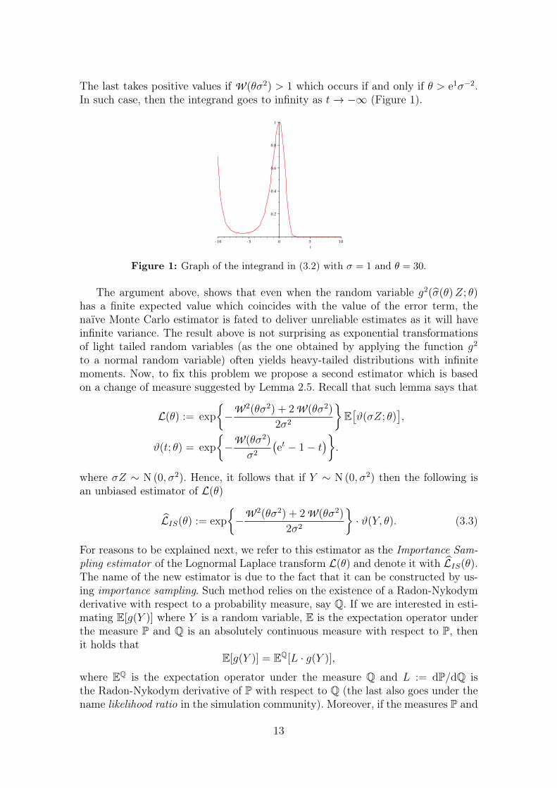
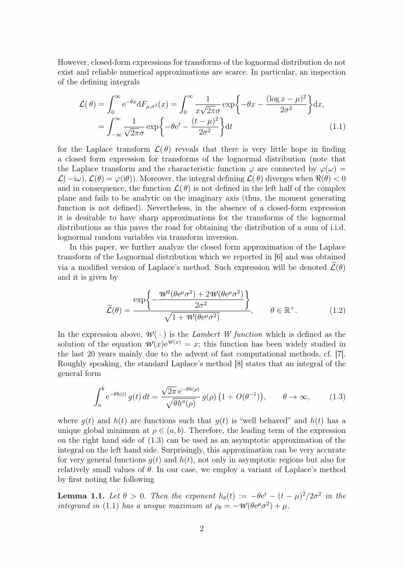
The last takes positive values if W (θσ2) > 1 which occurs if and only if θ > e1σ−2.In such case, then the integrand goes to infinity as t→ −∞ (Figure 1).

Figure 1: Graph of the integrand in (3.2) with σ = 1 and θ = 30.

The argument above, shows that even when the random variable g2(σ(θ)Z; θ)has a finite expected value which coincides with the value of the error term, thenaïve Monte Carlo estimator is fated to deliver unreliable estimates as it will haveinfinite variance. The result above is not surprising as exponential transformationsof light tailed random variables (as the one obtained by applying the function g2

to a normal random variable) often yields heavy-tailed distributions with infinitemoments. Now, to fix this problem we propose a second estimator which is basedon a change of measure suggested by Lemma 2.5. Recall that such lemma says that

L(θ) := exp

{−W 2(θσ2) + 2 W (θσ2)

2σ2

}E[ϑ(σZ; θ)

],

ϑ(t; θ) = exp

{−W (θσ2)

σ2

(et − 1− t

)}.

where σZ ∼ N (0, σ2). Hence, it follows that if Y ∼ N (0, σ2) then the following isan unbiased estimator of L(θ)

LIS(θ) := exp

{−W 2(θσ2) + 2 W (θσ2)

2σ2

}· ϑ(Y, θ). (3.3)

For reasons to be explained next, we refer to this estimator as the Importance Sam-pling estimator of the Lognormal Laplace transform L(θ) and denote it with LIS(θ).The name of the new estimator is due to the fact that it can be constructed by us-ing importance sampling. Such method relies on the existence of a Radon-Nykodymderivative with respect to a probability measure, say Q. If we are interested in esti-mating E[g(Y )] where Y is a random variable, E is the expectation operator underthe measure P and Q is an absolutely continuous measure with respect to P, thenit holds that

E[g(Y )] = EQ[L · g(Y )],

where EQ is the expectation operator under the measure Q and L := dP/dQ isthe Radon-Nykodym derivative of P with respect to Q (the last also goes under thename likelihood ratio in the simulation community). Moreover, if the measures P and

13

Q are absolutely continuous, then the Radon-Nykodym derivative/likelihood ratiois simply the ratio of the corresponding density functions. Hence, if Y is simulatedaccording to Q, then L·g(Y ) serves as an unbiased estimator of the quantity E[g(Y )].

Notice that the importance sampling methodology ensures that the new estima-tor is unbiased; also in most of the cases it will have a different variance. However,there is no guarantee that the new variance is smaller and that of course dependson an adequate selection of the importance distribution.

In our setting, we want to estimate the quantity E[g(Y ; θ)] where Y ∼ N (0, σ2(θ))and g is the function given it Proposition 2.1. Thus, we select Q in such way thatY ∼ N (0, σ2). It turns out that the the likelihood ratio is equal to

L(y) :=f0,σ2(θ)(y)

f0,σ2(y)=√

1 + W (θσ2) exp

{−W (θσ2)

y2

2σ2

}

where fµ,σ2(y) denotes the density of the normal distribution N(µ, σ2). Then it fol-lows that

L · g(y; θ) =√

1 + W (θσ2) exp

{−W (θσ2)

y2

2σ2

}

· exp

{−W (θσ2)

σ2

(ey − (1 + y + y2/2)

)}

=√

1 + W (θσ2) exp

{− W (θσ2)

σ2

(ey − (1 + y)

)}

=√

1 + W (θσ2) · ϑ(y; θ).

This argument confirms that the estimator LIS(θ) is an importance sampling esti-mator with respect to the Naïve Monte Carlo estimator LN(θ) and with N(0, σ2)

as importance sampling distribution. Moreover, it turns out that LIS(θ) achieveslogarithmic efficiency:

Proposition 3.2. LIS(θ) is an unbiased estimator of the Laplace transform of thelognormal distribution LN(0, σ2). Moreover, it is logarithmic efficient as θ →∞.

Proof of Proposition 3.2. By construction, LIS(θ) is an unbiased estimator of L(θ).To prove logarithmic efficiency we use the equivalence in Lemma 2.5 and the asymp-totic relation in Corollary 2.3 to verify the following equivalence

limθ→∞

Var[L2(θ)]

L2−ε(θ)= lim

θ→∞

L2(θ)(1 + W (θσ2)

)· Var[ϑ(Y ; θ)]

L2−ε(θ)

= limθ→∞Lε(θ)

(1 + W (θσ2)

)· Var[ϑ(Y ; θ)],

where L(θ) is the asymptotically equivalent approximation of L(θ) given by theLaplace’s method. Since ϑ2(y; θ) ≤ 1 we have the following bounds

limθ→∞Lε(θ)

(1 + W (θσ2)

)E[ϑ2(σZ; θ)] ≤ lim

θ→∞Lε(θ)(1 + W (θσ2)) = 0.

The last limit is straightforward to verify by inserting the formula for L(θ) given in(1.2) and checking that the term 1 + W (θσ2) is asymptotically bounded by Lε(θ)for all ε > 0.

14

Algorithm. The following generates a single replicate of the IS estimator.

1. Simulate Y ∼ N (0, σ2).

2. Compute ϑ(Y ; θ) = exp

{− W (θσ2)

σ2

(eY − 1− Y

)}.

3. Return LIS(θ) := exp

{−W 2(θσ2) + 2 W (θσ2)

2σ2

}ϑ(Y ; θ).

4 Numerical examples

In this section we investigate the numerical performance of our proposals and com-pare them against several approximations available in the literature; we furtherdiscuss the quality of the approximates. First we conduct separate investigations onapproximations of the Laplace transform and the characteristic function. Secondly,we corroborate empirically the efficiency properties of the Monte Carlo estimatorsconsidered in this paper.

4.1 Approximations of the Laplace transform

We first considered approximations of the Laplace transform of the lognormal distri-butions. For that purpose we examined the proposals of Barakat [9], Gubner [12] andTellambura/Senaratne [13] (further discussion on these results can be found in thelast section of this paper). These proposals were originally designed for approximat-ing the characteristic function; however, one can make the appropriate comparisonsby using the relation L(iθ) = ϕ(θ). We compared these approximations against ourclosed form expression (1.2) which was referred as LM-approximation. We decidedto use the importance sampling Monte Carlo estimator suggested in section 3 asbenchmark of comparison; recall that we employed the name IS estimator to referto it. We have employed 108 replications for each estimate. In the examples below,we present tables with the values of both the approximation and the relative errorswith respect to the IS estimator. The latter is defined as

Relative Error =Approximation− IS estimate

IS estimate.

It is important to remark that for the approximations suggested by Gubner andTellambura-Senaratne we employed the Matlab codes provided by the authors.

Example 1. For our first example we have used a value of σ = 0.25 (this value isemployed in the numerical results presented in the paper of Barakat [9] and usedhere for corroboration purposes). The results are presented in Table 1.

For this example, the results of Gubner were excluded since the correspondingalgorithm delivered values which were much larger than 1. The method of Tellam-bura/Senaratne also produced unreliable results: notice for instance that it producesan estimate of L(0) which has an error of about 5% (recall that L(0) = 1). In con-trast, our two proposals delivered very similar results, thus confirming that theLaplace’s method can produce indeed very sharp approximations of the Laplace

15

Table 1: Approximated Values of L(θ) with σ = 0.25.

θ IS Monte Carlo LM approximation Tellambura/Senaratne Barakat

0.0 1.000000 1.000000 0.945115 1.0000000.4 0.670006 0.670006 0.633173 0.6700060.8 0.449189 0.449190 0.424455 0.4491891.2 0.301335 0.301336 0.284715 0.3013351.6 0.202274 0.202275 0.191099 0.2022742.0 0.135862 0.135862 0.128344 0.135862

transform of the lognormal distribution. The results of Barakat coincide with ourresults, thus reassuring the sharpness of our methods for small values of σ. Table 2below shows the relative errors of the estimators. It is noted that the method ofTellambura/Seranatne underestimates the real values with errors of about 5.5% noonly in a neighborhood of 0 but all across the domain of the transform.

Table 2: Relative Errors of L(θ) with σ = 0.25.

θ LM approximation Tellambura/Senaratne Barakat

0.0 0.000000× 100 −0.054885 0.000000× 100

0.4 7.986949× 10−7 −0.054974 4.080170× 10−8

0.8 2.009580× 10−6 −0.055064 5.047547× 10−7

1.2 2.381985× 10−6 −0.055154 1.410071× 10−7

1.6 2.876162× 10−6 −0.055245 −9.037186× 10−8

2.0 2.906645× 10−6 −0.055337 −7.750253× 10−7

Example 2. In the second example we consider a value of σ = 1. The results arepresented in Table 3.

Table 3: Approximated Values of L(θ) with σ = 1.

θ IS Monte Carlo LM approximation Tellambura Barakat Gubner

0.0 1.000000 1.000000 1.000000 1.000000 1.0000000.4 0.616293 0.624119 0.616284 0.642997 0.6157470.8 0.440037 0.445053 0.440053 0.673959 0.4345381.2 0.335214 0.338399 0.335201 −1.753636 0.3199621.6 0.265606 0.267730 0.265610 −50.847370 0.2311622.0 0.216313 0.217758 0.216309 −596.161998 0.279931

One of the most notorious aspects of this case is that the approximation ofBarakat deteriorates rapidly. The method of Gubner delivers better results but stillwith large errors. The algorithm of Tellambura seems to be the one delivering thebest results. In the case of our LM approximation, it delivers sensible results whichdoes not seem to deteriorate as the value of θ increases; nevertheless, it seems thatthis closed form approximation looses accuracy as σ increases. These observationsare reaffirmed after examining the relative errors in Table 4.

16

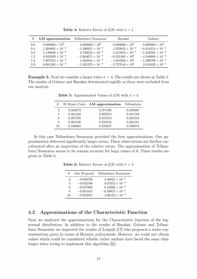
Table 4: Relative Errors of L(θ) with σ = 1.

θ LM approximation Tellambura/Senaratne Barakat Gubner

0.0 0.000000× 100 0.000000× 100 0.000000× 100 0.000000× 100

0.4 1.269892× 10−2 −1.396821× 10−5 4.333043× 10−2 −8.854354× 10−4

0.8 1.139909× 10−2 3.720053× 10−5 5.315953× 10−1 −1.249595× 10−2

1.2 9.502939× 10−3 −3.903671× 10−5 −6.231395× 100 −4.549968× 10−2

1.6 7.997354× 10−3 1.402916× 10−5 −1.924392× 102 −1.296799× 10−1

2.0 6.681295× 10−3 −1.925373× 10−5 −2.757016× 103 2.941032× 10−1

Example 3. Next we consider a larger value σ = 4. The results are shown in Table 5.The results of Gubner and Barakat deteriorated rapidly so these were excluded fromour analysis.

Table 5: Approximated Values of L(θ) with σ = 4.

θ IS Monte Carlo LM approximation Tellambura

2 0.382672 0.371296 0.3826854 0.321163 0.307613 0.3211946 0.287195 0.273413 0.2872198 0.264198 0.250553 0.264181

10 0.246962 0.233637 0.246974

In this case Tellambura/Senaratne provided the best approximations. Our ap-proximation delivered significantly larger errors. These observations are further cor-roborated after an inspection of the relative errors. The approximation of Tellam-bura/Senaratne seems to be remain accurate for large values of θ. These results aregiven in Table 6.

Table 6: Relative Errors of L(θ) with σ = 4.

θ Our Proposal Tellambura/Senaratne

2 −0.029728 3.36825× 10−5

4 −0.042190 9.65352× 10−5

6 −0.047989 8.44206× 10−5

8 −0.051645 −6.49857× 10−5

10 −0.053957 4.96133× 10−5

4.2 Approximations of the Characteristic Function

Next we analyzed the approximations for the Characteristic function of the log-normal distribution. In addition to the results of Barakat, Gubner and Tellam-bura/Senaratne we inspected the results of Leipnik [17] who proposed a series rep-resentations given in terms of Hermite polynomials. However, we could not obtainvalues which could be considered reliable (other authors have faced the same chal-lenges when trying to implement this algorithm [5]).

17

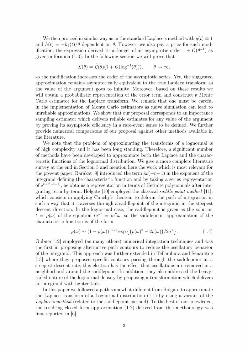
Example 4. For our single example we considered a value of σ = 0.5. The graphsof the real and imaginary part of ϕ(ω) are shown in Figure 2. Our approximationand the Tellambura/Senaratne are indistinguishable in the graphs as these are veryaccurate. However, the approximation of Barakat deteriorates in regions away from 0.This phenomena could be explained by the fact that the Barakat approximationis obtained by truncating a converging series. In particular, we observed that theBarakat approximation also deteriorates as the value of σ increases thus requiringan even larger amount of series terms.

−20 −15 −10 −5 0 5 10 15 20−0.4

−0.2

0

0.2

0.4

0.6

0.8

1Real

LM approximation

Tellambura

Barakat

−20 −15 −10 −5 0 5 10 15 20−0.8

−0.6

−0.4

−0.2

0

0.2

0.4

0.6

0.8Imaginary

LM approximation

Tellambura

Barakat

Figure 2: Real and imaginary parts of the Characteristic function of the Lognormal forσ = 0.5.

We conducted similar experiments for alternative values of σ and we obtainedsimilar conclusions as in the case of the Laplace transform. For very small values ofthe σ, the approximation of Tellabura/Senaratne delivers unreliable approximationsand sometimes it fails to converge. In the same case, the algorithm of Barakat and ourproposal deliver very sharp approximates. As the value of σ increases, the proposalof Barakat deteriorates rapidly. Our proposal loses some precision but still deliveredsensible approximations. For moderately large values of σ it is the algorithm ofTellambura/Seranarte the one which produces the best results.

4.3 Efficient Monte Carlo

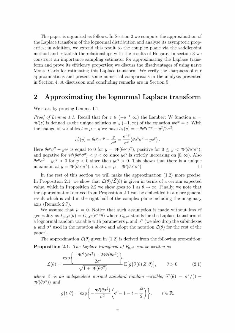
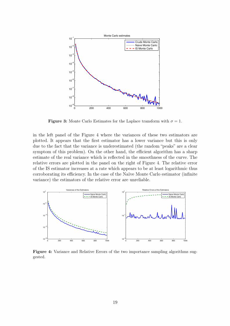
Example 5. In this example we contrast the three estimators discussed in this pa-per: Crude Monte Carlo, Naïve Monte Carlo and Efficient Monte Carlo. We selecteda value of σ = 1. In the three cases we have employed R = 108 replications. Fig-ure 3 shows the estimates provided by the three methods in logarithmic scale. It isobserved that Crude Monte Carlo provides a reasonable approximation of the trueLaplace transform for small values of the argument; however, as the value of θ in-creases, the quality of the crude estimate deteriorates as the relative error increases(this explains the jiggled nature of the curve). On the other hand, it appears thatthe two importance sampling methods discussed here provide sharp approximationsas their values are very close to each other (the curves are indistinguishable fromeach other).

However, one of the two importance sampling estimators (Naïve Monte Carlo)has an infinite variance, so it can provide unreliable estimates. This effect is noted

18

0 200 400 600 800 100010

−9

10−8

10−7

10−6

10−5

10−4

10−3

10−2

10−1

Monte Carlo estimates

Crude Monte Carlo

Naive Monte Carlo

IS Monte Carlo

Figure 3: Monte Carlo Estimates for the Laplace transform with σ = 1.

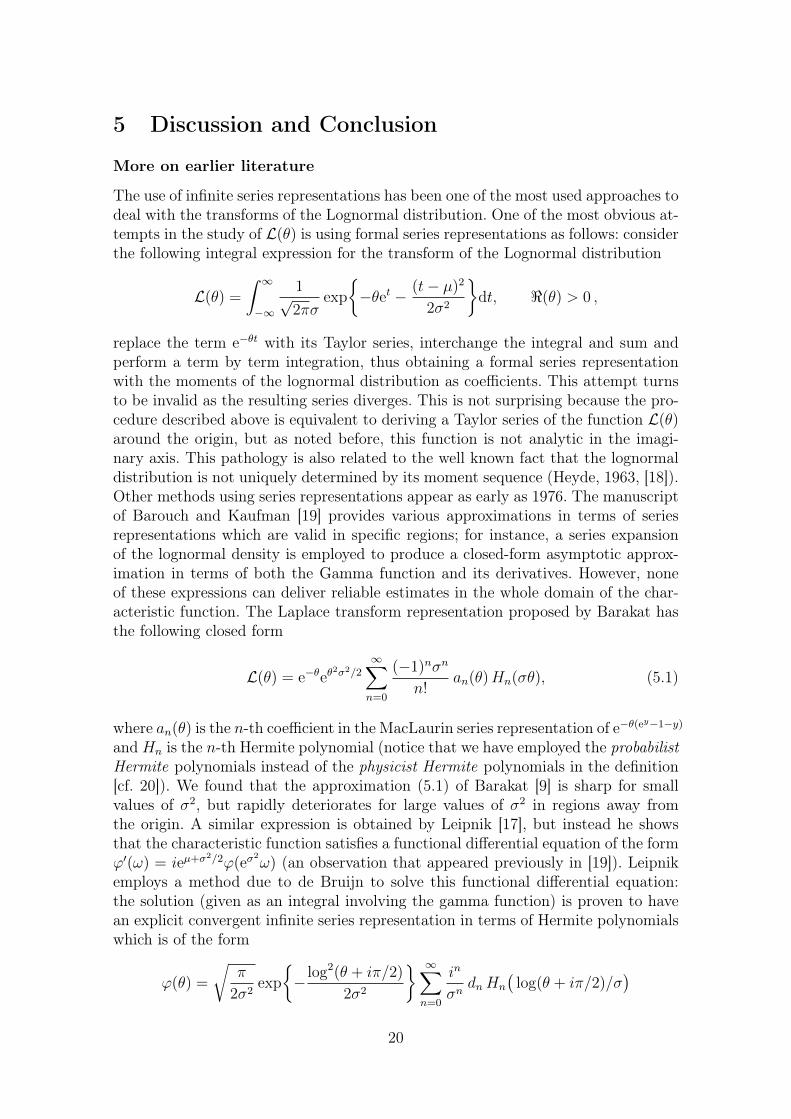
in the left panel of the Figure 4 where the variances of these two estimators areplotted. It appears that the first estimator has a lower variance but this is onlydue to the fact that the variance is underestimated (the random “peaks” are a clearsymptom of this problem). On the other hand, the efficient algorithm has a sharpestimate of the real variance which is reflected in the smoothness of the curve. Therelative errors are plotted in the panel on the right of Figure 4. The relative errorof the IS estimator increases at a rate which appears to be at least logarithmic thuscorroborating its efficiency. In the case of the Naïve Monte Carlo estimator (infinitevariance) the estimators of the relative error are unreliable.

0 200 400 600 800 100010

−20

10−15

10−10

10−5

100

Variances of the Estimators

Naive Monte Carlo

IS Monte Carlo

0 200 400 600 800 100010

−2

10−1

100

Relative Errors of the Estimators

Naive Monte Carlo

IS Monte Carlo

Figure 4: Variance and Relative Errors of the two importance sampling algorithms sug-gested.

19

5 Discussion and Conclusion

More on earlier literature

The use of infinite series representations has been one of the most used approaches todeal with the transforms of the Lognormal distribution. One of the most obvious at-tempts in the study of L(θ) is using formal series representations as follows: considerthe following integral expression for the transform of the Lognormal distribution

L(θ) =

∫ ∞

−∞

1√2πσ

exp

{−θet − (t− µ)2

2σ2

}dt, <(θ) > 0 ,

replace the term e−θt with its Taylor series, interchange the integral and sum andperform a term by term integration, thus obtaining a formal series representationwith the moments of the lognormal distribution as coefficients. This attempt turnsto be invalid as the resulting series diverges. This is not surprising because the pro-cedure described above is equivalent to deriving a Taylor series of the function L(θ)around the origin, but as noted before, this function is not analytic in the imagi-nary axis. This pathology is also related to the well known fact that the lognormaldistribution is not uniquely determined by its moment sequence (Heyde, 1963, [18]).Other methods using series representations appear as early as 1976. The manuscriptof Barouch and Kaufman [19] provides various approximations in terms of seriesrepresentations which are valid in specific regions; for instance, a series expansionof the lognormal density is employed to produce a closed-form asymptotic approx-imation in terms of both the Gamma function and its derivatives. However, noneof these expressions can deliver reliable estimates in the whole domain of the char-acteristic function. The Laplace transform representation proposed by Barakat hasthe following closed form

L(θ) = e−θeθ2σ2/2

∞∑

n=0

(−1)nσn

n!an(θ)Hn(σθ), (5.1)

where an(θ) is the n-th coefficient in the MacLaurin series representation of e−θ(ey−1−y)

and Hn is the n-th Hermite polynomial (notice that we have employed the probabilistHermite polynomials instead of the physicist Hermite polynomials in the definition[cf. 20]). We found that the approximation (5.1) of Barakat [9] is sharp for smallvalues of σ2, but rapidly deteriorates for large values of σ2 in regions away fromthe origin. A similar expression is obtained by Leipnik [17], but instead he showsthat the characteristic function satisfies a functional differential equation of the formϕ′(ω) = ieµ+σ

2/2ϕ(eσ2ω) (an observation that appeared previously in [19]). Leipnik

employs a method due to de Bruijn to solve this functional differential equation:the solution (given as an integral involving the gamma function) is proven to havean explicit convergent infinite series representation in terms of Hermite polynomialswhich is of the form

ϕ(θ) =

√π

2σ2exp

{− log2(θ + iπ/2)

2σ2

} ∞∑

n=0

in

σndnHn

(log(θ + iπ/2)/σ

)

20

where dn are the coefficients in the MacLaurin series representation of the recip-rocal of the Gamma function Γ−1(y + 1). Leipnik includes a recursive formula forcalculating the coefficients dn in terms of the Euler’s constant and the RiemannZeta function; this recursion facilitates the calculation of this series representation.However, the solution of the functional differential equation cannot be extended tothe whole complex plane, so it appears that this approximation only applies forthe characteristic function (in fact, we were not able to obtain a reliable numericalestimate using any of these formulae).

In his study of the characteristic function, cf. [10], Holgate applied the Lagrangeinversion theorem to the equivalence te−t = iσ2ω to obtain an asymptotic series rep-resentation of the saddle point function ρ(ω), which inserted into expression (1.4)provides a representation of the function ϕ(ω) in terms of an asymptotic infiniteseries. However, the resulting series oscillates wildly and cannot provide a reliablenumerical approximations. Finally, another interesting and somewhat different ap-proach which delivers closed-form expressions is given by Rossberg [21], who pro-vides a representation of general Laplace transforms in terms of a 2-fold convolutioninvolving the cdf of the random variable of interest.

Numerical integration methods have also received a good deal of attention andmost of these have been developed in parallel with the analytic approximations dis-cussed above. One of the earliest references is [16], where the performance of variousstandard integration methods is analyzed. It is remarked there that approximatingthe characteristic function via numerical integration is very challenging due to theoscillatory nature of the term eiωt and the heavy-tailed nature of the lognormal den-sity [cf. 22]. This fact has been further discussed in several other papers [9, 12, 16]).An obvious approach to deal with the oscillations is to employ complex analytictechniques: besides the paper of Holgate [10] where the saddlepoint methodologyis exploited, it seems that Gubner [12] was the first in proposing alternative pathcontours to reduce the oscillatory behavior of the integrand, as followed up by Tel-lambura and Senaratne [13] where they proposed specific contours passing throughthe saddlepoint at a steepest descent rate; this choice has the effect that oscillationsare removed in a neighborhood around the saddlepoint. In addition, they also ad-dress the heavy-tailed nature of the lognormal density by proposing a transformationwhich delivers an integrand with lighter tails.

Summary of the paper

A closed form expression of the Laplace transform of the lognormal distribution doesnot exist. Providing a reliable approximation is a difficult problem since traditionalapproximation methods fail mainly due to the fact that the Lognormal distributionis heavy-tailed and its transforms are not analytic in the origin. In this paper weproposed a closed form approximation of the Laplace transform which is obtained viaa modified version of the classic asymptotic Laplace’s method. The main result is adecomposition of the Laplace transform which delivers a closed form approximationof the Laplace transform and an expression of the exact error. The last turns to beuseful to prove the asymptotic equivalence of the proposed approximation. Moreover,since the error term is given in a probabilistic representation it turns out to beconvenient for analysis.

21

In addition, we constructed a Monte Carlo estimator of the Laplace transform ofthe Lognormal distribution. This estimator is based on the probabilistic represen-tation of the error term obtained via the modified version of the Laplace’s method.We prove the efficiency of this estimator. In contrast, we illustrate that the Crudeand Naïve Monte Carlo implementations can deliver unreliable estimates for largevalues of the argument.

Finally, we conducted numerical experiments where we compared our proposalsagainst other approximations available in the literature. We found that most ap-proximations are very sensible for different values of σ. The method of Tellamburais one of the most precise; however, it delivers unreliable results for small values ofσ and sometimes it fails to converge. The proposal of Barakat can deliver sharp re-sults for small values of σ but fails for large values of the argument. Our closed-formLM expression delivers approximations which remain precise all over the domain ofthe transform; in particular, it tends to be more precise for small values of σ . Anattractive feature of our proposal is its simple closed-form.

In contrast, we showed that our efficient IS Monte Carlo estimator is the onlymethod which delivered reliable sharp results for any combination of values of theparameters σ and θ. In particular, it remains sharp in asymptotic regions as it isbased on an asymptotic method. In addition it has a simple form and it is easy toimplement. Moreover, it does not have convergence issues. Overall, this seems to bethe best available option to approximate the Laplace transform of the Lognormaldistribution.

Work in progress

One obvious way to go is to apply our results to approximate the density andcumulative distribution function of a sum of independent random variables. Theobvious idea is via transform inversion, but we could also apply the saddlepointmethodology to obtain approximations in the left tail via Escher and Legendre-Fenchel transforms (note that the left tail is of particular importance in financebecause of its interpretation related to, say, portfolio loss). In addition, one couldalso construct reliable efficient Monte Carlo estimators based on this approximation.Finally, Laplace transforms of correlated lognormals could also be explored.

References

[1] I. Aitchison and J. A. C. Brown, The lognormal distribution with special reference toits uses in economics. Cambridge: Cambridge University Press, 1957.

[2] E. L. Crow and K. Shimizu, Lognormal distributions: theory and applications. NewYork: Marcel Dekker Inc., 1988.

[3] N. L. Johnson, S. Kotz, and N. Balakrishnan, Continuous Univariate Distributions,vol. 1. New York: Wiley, 2 ed., 1994.

[4] E. Limpert, W. A. Stahel, and M. Abbt, “Log-normal distributions across the sciences:Keys and clues,” BioScience, vol. 51, pp. 341–352, 2001.

22

[5] D. Dufresne, “Sums of lognormals,” in Actuarial Research Conference Proceedings,2008.

[6] L. Rojas-Nandayapa, Risk probabilities: Asymptotics and Simulation. PhD thesis,Aarhus University, 2008.

[7] R. M. Corless, G. H. Gonnet, D. E. G. Hare, D. J. Jeffrey, and D. E. Knuth, “On theLambert W function,” Advances in Computational Mathematics, vol. 5, pp. 329–359,1996.

[8] N. G. de Bruijn, Asymptotic Methods in Analysis. Courier Dover Publications, 1970.

[9] R. Barakat, “Sums of independent lognormally distributed random variables,” Journalof the Optical Society of America, vol. 66, pp. 211–216, 1976.

[10] P. Holgate, “The lognormal characteristic function,” Communications in Statistical-Theory and Methods, vol. 18, pp. 4539–4548, 1989.

[11] J. L. Jensen, Saddlepoint Approximations. Oxford: Oxford Science Publications, 1994.

[12] J. A. Gubner, “A new formula for lognormal characteristic functions,” IEEE Transac-tions on Vehicular Technology, vol. 55, no. 5, pp. 1668–1671, 2006.

[13] C. Tellambura and D. Senaratne, “Accurate computation of the MGF of the lognor-mal distribution and its application to sum of lognormals,” IEEE Transactions onCommunications, vol. 58, pp. 1568–1577, 2010.

[14] R. W. Butler, Saddlepoint Approximations with Applications. Cambridge UniversityPress, 2007.

[15] C. G. Small, Expansions and Asymptotics for Statistics. Chapman & Hall/CRC, 2013.

[16] N. C. Beaulieu and Q. Xie, “An optimal lognormal approximation to lognormal sumdistributions,” IEEE Transactions on Vehicular Technology, vol. 53, no. 2, pp. 479–489, 2004.

[17] R. B. Leipnik, “On lognormal random variables: I. the characteristic function,” Journalof the Australian Mathematical Society Series B, vol. 32, pp. 327–347, 1991.

[18] C. Heyde, “On a property of the lognormal distribution,” J. Roy. Statist. Soc. Ser. B,vol. 29, pp. 392–393, 1963.

[19] E. Barouch and G. M. Kaufman, “On sums of lognormal random variables.” Workingpaper. A. P. Sloan School of Management, MIT., 1976.

[20] M. Abramowitz and I. Stegun, Handbook of Mathematical Functions: With Formulas,Graphs, and Mathematical Tables. Applied mathematics series, Dover Publications,1964.

[21] A. G. Rossberg, “Laplace transforms or probability distributions and their inversionsare easy on logarithmic scales,” Journal of Applied Probabilty, vol. 45, pp. 531–541,2008.

[22] S. Foss, D. Korshunov, and S. Zachary, An introduction to heavy-tailed and subexpo-nential distributions. Springer, 2011.

23