Cooperative positioning studies based on WLANs
117
TERY OSMAR CAISAGUANO VÁSQUEZ COOPERATIVE POSITIONING STUDIES BASED ON WIRELESS LOCAL AREA NETWORKS (WLANs) Master’s thesis Examiners: Adj. Prof. Elena Simona Lohan Francescantonio Della Rosa Examiner and topic approved by the Faculty Council of Computing and Electrical Engineering. 15 January 2014
Transcript of Cooperative positioning studies based on WLANs
TERY OSMAR CAISAGUANO VÁSQUEZ
COOPERATIVE POSITIONING STUDIES BASED ON WIRELESS
LOCAL AREA NETWORKS (WLANs)
Master’s thesis
Examiners: Adj. Prof. Elena Simona Lohan
Francescantonio Della Rosa
Examiner and topic approved by the Faculty Council of
Computing and Electrical Engineering.
15 January 2014
I
ABSTRACT
TAMPERE UNIVERSITY OF TECHNOLOGY
CAISAGUANO VÁSQUEZ, TERY OSMAR: Cooperative positioning studies based
on Wireless Local Area Networks (WLANs)
Master of Science Thesis, 84 pages, 18 Appendix pages
15 January 2014
Major subject: Communications Engineering
Examiners: Adj. Prof. Elena Simona Lohan and Francescantonio Della Rosa
Keywords: Indoor Positioning, WLAN, Fingerprinting, Path Loss, Non-Cooperative
Positioning, Cooperative Positioning, Wi-Fi, Received Signal Strength.
Location information and location-based service have gained importance in recent
years because, based on their concept, a new business market has been opened which
encompass emergency services, security, monitoring, tracking, logistics, etc. Nowadays,
the most developed positioning systems, namely the Global Navigation Satellite Systems
(GNSS), are meant for outdoor use. In order to integrate outdoor and indoor localization
in the same mobile application, several lines of research have been created for the purpose
of investigating the possibility of wireless network technologies and of overcoming the
challenges faced by GNSS in performing localization and navigation in indoor
environments. The benefit in using wireless networks is that they provide a minimally
invasive solution which is based on software algorithms that can be implemented and
executed in the Mobile Station (MS) or in a Location Server connected to the network.
This thesis focuses on the development of localization approaches based on Received
Signal Strength (RSS) and applied in WLANs. Such approaches demonstrated in recent
research advances that RSS-based localization algorithms are the simplest existing
approaches due to the fact that the RSSs are most accessible existing measurements. RSS
measurements can be used with two main algorithms, which are addressed in this thesis:
Fingerprinting method (FP) and Pathloss method (PL). These two methods can be applied
in both cooperative and non-cooperative algorithms. Such algorithms are evaluated here
in terms of Root Mean Square Error (RMSE) for both simulated and real-field data.

II
PREFACE
I would like to show my gratitude to all those who in one way or another, have contributed
to the realization of this master thesis.
I acknowledge Adj. Prof. Elena Simona Lohan, who took me in and made me feel
comfortable during the research stage and gave me the opportunity to carry out my master
thesis. Her patience and invaluable help to my research was much appreciated.
Also I want to give thanks to Francesantonio Della Rosa for his help and great advice.
I would not be where I am today without my family, who I have to give thanks to for their
unconditional support during all my university studies. In the same note, I also
acknowledge my girlfriend Päivi Erkkilä, who helped me a lot throughout this project.
Tampere,
Tery Osmar Caisaguano Vásquez
III
TABLE OF CONTENTS
ABSTRACT ..................................................................................................................... I
PREFACE ....................................................................................................................... II
TABLE OF CONTENTS ............................................................................................. III
LIST OF SYMBOLS ................................................................................................... VI
LIST OF ACRONYMS ............................................................................................ VIII
1 INTRODUCTION ................................................................................................... 1
MOTIVATION .................................................................................................................2
AUTHOR’S CONTRIBUTIONS ..........................................................................................3
OUTLINE .......................................................................................................................3
2 WIRELESS NETWORKS ..................................................................................... 5
WIRELESS PERSONAL AREA NETWORKS (WPAN) ......................................................8
2.1.1 Bluetooth ..................................................................................................................9
2.1.2 ZigBee ....................................................................................................................12
WIRELESS LOCAL AREA NETWORKS (WLAN) ..........................................................15
2.2.1 IEEE 802.11 ...........................................................................................................17
2.2.1.1 Network modes ......................................................................................................... 18
2.2.1.2 Shared media access ................................................................................................. 20
2.2.1.3 Physical layers variances .......................................................................................... 23
2.2.2 IEEE 802.11b .........................................................................................................24
2.2.3 IEEE 802.11a .........................................................................................................24
2.2.4 IEEE 802.11g .........................................................................................................25
2.2.5 IEEE 802.11n .........................................................................................................25
WIRELESS METROPOLITAN AREA NETWORKS (WMAN) ..........................................25
2.3.1 WiMAX ...................................................................................................................26
2.3.1.1 Network modes ......................................................................................................... 27
2.3.1.2 Network elements ..................................................................................................... 29
2.3.1.3 Shared media access ................................................................................................. 29
2.3.1.4 Physical layers variances .......................................................................................... 31
SUMMARY ...................................................................................................................32
3 NON-COOPERATIVE LOCALIZATION METHODS IN WIRELESS
NETWORKS ................................................................................................................. 33
TIME BASED LOCALIZATION .......................................................................................34
3.1.1 Time of Arrival (TOA) ............................................................................................35
TABLE OF CONTENTS IV
3.1.2 Time Difference of Arrival (TDOA) .......................................................................35
3.1.3 Round-Trip Time of Flight (RTOF) ........................................................................36
ANGLE BASED LOCALIZATION ....................................................................................37
RECEIVED SIGNAL STRENGTH BASED LOCALIZATION (RSS) .....................................37
3.3.1 Cell-ID based localization .....................................................................................38
3.3.2 Fingerprinting based localization (FP) .................................................................39
3.3.2.1 Training/Offline phase .............................................................................................. 40
3.3.2.2 Estimation/Online phase ........................................................................................... 41
3.3.3 Pathloss-based localization (PL) ...........................................................................42
3.3.3.1 Training/Offline phase .............................................................................................. 44
3.3.3.2 Estimation/Online phase ........................................................................................... 47
4 COOPERATIVE LOCALIZATION METHODS IN WIRELESS
NETWORKS ................................................................................................................. 49
CENTRALIZED COOPERATIVE APPROACH ...................................................................50
4.1.1 Semi-Definite Programming (SDP) .......................................................................51
4.1.2 Multidimensional Scaling (MDS) ...........................................................................52
4.1.3 Maximum-Likelihood Estimation (MLE) ...............................................................53
DISTRIBUTED COOPERATIVE APPROACH ....................................................................53
4.2.1 Lateration ...............................................................................................................54
4.2.2 Nonparametric Belief Propagation (NBP) .............................................................54
4.2.3 Non-Bayesian Estimators .......................................................................................55
PROPOSED COOPERATIVE APPROACH .........................................................................55
5 INVESTIGATED APPROACHES AND COMPARATIVE RESULTS ......... 58
NON-COOPERATIVE METHODS ....................................................................................60
5.1.1 Fingerprinting approach ........................................................................................60
5.1.1.1 Transmit power and pathloss exponent from each AP .............................................. 61
5.1.1.2 Shadowing estimation ............................................................................................... 61
5.1.1.3 Device map location ................................................................................................. 62
5.1.1.4 RMSE estimation ...................................................................................................... 63
5.1.1.5 Fingerprinting power maps ....................................................................................... 64
5.1.2 Pathloss approach ..................................................................................................65
5.1.2.1 Transmit power and pathloss exponent estimation from each AP ............................ 65
5.1.2.2 Shadowing estimation ............................................................................................... 66
5.1.2.3 Device map location ................................................................................................. 67
5.1.2.4 RMSE estimation ...................................................................................................... 68
5.1.2.5 Empirical radio map .................................................................................................. 69
5.1.3 Comparison between both approaches via Monte Carlo simulation .....................70
COOPERATIVE METHOD ..............................................................................................72
5.2.1 Fingerprinting approach ........................................................................................73
5.2.2 Pathloss approach ..................................................................................................75
5.2.3 Experimental results ...............................................................................................75
6 CONCLUSIONS AND OPEN DIRECTIONS ................................................... 78
7 REFERENCES ...................................................................................................... 79

TABLE OF CONTENTS V
APPENDIX I: COOPERATIVE AND NON-COOPERATIVE LOCALIZATION
VIA FP APPROACH .................................................................................................... 85
APPENDIX II: COOPERATIVE AND NON-COOPERATIVE LOCALIZATION
VIA PL APPROACH .................................................................................................... 94
VI
LIST OF SYMBOLS
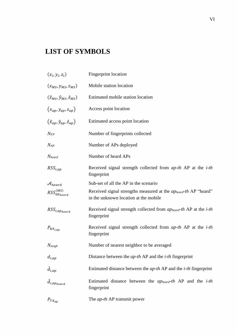
(𝑥𝑖, 𝑦𝑖 , 𝑧𝑖) Fingerprint location
(𝑥𝑀𝑆, 𝑦𝑀𝑆, 𝑧𝑀𝑆) Mobile station location
(�̂�𝑀𝑆, �̂�𝑀𝑆, �̂�𝑀𝑆) Estimated mobile station location
(𝑥𝑎𝑝, 𝑦𝑎𝑝, 𝑧𝑎𝑝) Access point location
(�̂�𝑎𝑝, �̂�𝑎𝑝, �̂�𝑎𝑝) Estimated access point location
NFP Number of fingerprints collected
NAP Number of APs deployed
Nheard Number of heard APs
𝑅𝑆𝑆𝑖,𝑎𝑝 Received signal strength collected from ap-th AP at the i-th
fingerprint
𝒜ℎ𝑒𝑎𝑟𝑑 Sub-set of all the AP in the scenario
𝑅𝑆𝑆𝑎𝑝ℎ𝑒𝑎𝑟𝑑
(𝑀𝑆) Received signal strengths measured at the apheard-th AP “heard”
in the unknown location at the mobile
𝑅𝑆𝑆𝑖,𝑎𝑝ℎ𝑒𝑎𝑟𝑑 Received signal strength collected from apheard-th AP at the i-th
fingerprint
𝑃𝑅𝑋𝑖,𝑎𝑝 Received signal strength collected from ap-th AP at the i-th
fingerprint
Nneigh Number of nearest neighbor to be averaged
𝑑𝑖,𝑎𝑝 Distance between the ap-th AP and the i-th fingerprint
�̂�𝑖,𝑎𝑝 Estimated distance between the ap-th AP and the i-th fingerprint
�̂�𝑖,𝑎𝑝ℎ𝑒𝑎𝑟𝑑 Estimated distance between the apheard-th AP and the i-th
fingerprint
𝑃𝑇𝑋𝑎𝑝 The ap-th AP transmit power
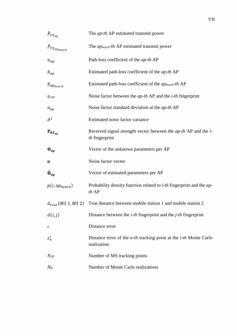
VII
�̂�𝑇𝑋𝑎𝑝 The ap-th AP estimated transmit power
�̂�𝑇𝑋𝑎𝑝ℎ𝑒𝑎𝑟𝑑 The apheard-th AP estimated transmit power
𝑛𝑎𝑝 Path-loss coefficient of the ap-th AP
�̂�𝑎𝑝 Estimated path-loss coefficient of the ap-th AP
�̂�𝑎𝑝ℎ𝑒𝑎𝑟𝑑 Estimated path-loss coefficient of the apheard-th AP
ηi,ap Noise factor between the ap-th AP and the i-th fingerprint
𝜎𝑎𝑝 Noise factor standard deviation at the ap-th AP
�̂�2 Estimated noise factor variance
𝐏𝑹𝑿𝒂𝒑 Received signal strength vector between the ap-th AP and the i-
th fingerprint
𝚯𝐚𝐩 Vector of the unknown parameters per AP
n Noise factor vector
�̂�𝐚𝐩 Vector of estimated parameters per AP
𝑝(𝑖, 𝑎𝑝ℎ𝑒𝑎𝑟𝑑) Probability density function related to i-th fingerprint and the ap-
th AP
𝑑𝑡𝑟𝑢𝑒(𝑀𝑆 1,𝑀𝑆 2) True distance between mobile station 1 and mobile station 2
𝑑(𝑖, 𝑗) Distance between the i-th fingerprint and the j-th fingerprint
ε Distance error
𝜀𝑛𝑖 Distance error of the n-th tracking point at the i-th Monte Carlo
realization
NTP Number of MS tracking points
NR Number of Monte Carlo realizations
VIII
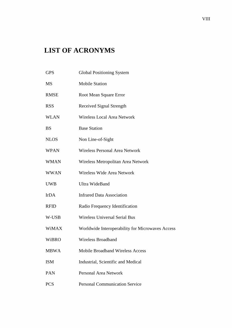
LIST OF ACRONYMS
GPS Global Positioning System
MS Mobile Station
RMSE Root Mean Square Error
RSS Received Signal Strength
WLAN Wireless Local Area Network
BS Base Station
NLOS Non Line-of-Sight
WPAN Wireless Personal Area Network
WMAN Wireless Metropolitan Area Network
WWAN Wireless Wide Area Network
UWB Ultra WideBand
IrDA Infrared Data Association
RFID Radio Frequency Identification
W-USB Wireless Universal Serial Bus
WiMAX Worldwide Interoperability for Microwaves Access
WiBRO Wireless Broadband
MBWA Mobile Broadband Wireless Access
ISM Industrial, Scientific and Medical
PAN Personal Area Network
PCS Personal Communication Service

IX
TDMA Time Division Multiple Access
MAC Media Access Control
FHSS Frequency-Hopping Spread Spectrum
FH-CDMA Frequency-Hopping Code Division Multiple Access
FSK Frequency-Shift Keying
LR-WPAN Low-Rate Wireless Personal Area Network
ASK Amplitude-Shift Keying
BPSK Binary Phase-Shift Keying
O-QPSK Offset Quadrature Phase-Shift Keying
DSSS Direct-Sequence Spread Spectrum
CSMA-CA Carrier Sense Multiple Access with Collision Avoidance
CCA Clear Channel Assessment
CS Carrier Sense
ED Energy Detection
GTS Guaranteed Time Slot
IEEE Institute of Electrical and Electronics Engineers
ETSI European Telecommunications Standards Institute
Wi-Fi Wireless Fidelity
WECA Wireless Ethernet Compatibility Alliance
AP Access Point
IEEE Institute of Electrical and Electronics Engineers
ETSI European Telecommunications Standards Institute
CSMA-CD Carrier Sense Multiple Access with Collision Detection
LLC Logical Link Control
X
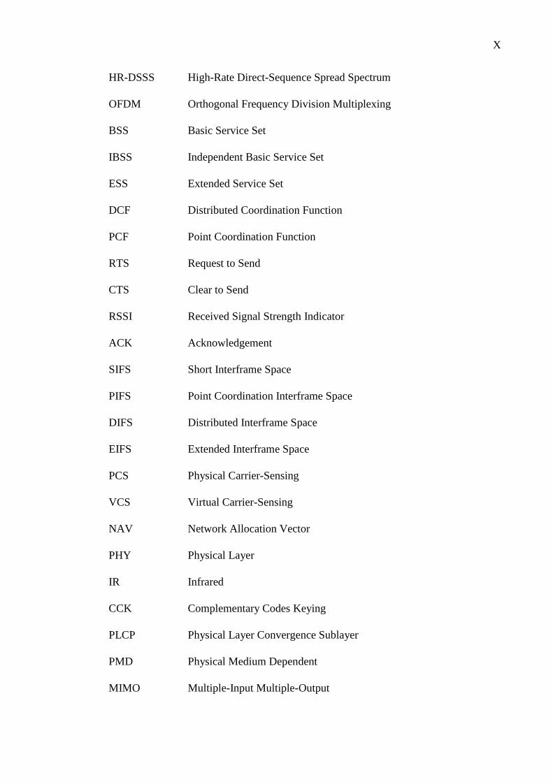
HR-DSSS High-Rate Direct-Sequence Spread Spectrum
OFDM Orthogonal Frequency Division Multiplexing
BSS Basic Service Set
IBSS Independent Basic Service Set
ESS Extended Service Set
DCF Distributed Coordination Function
PCF Point Coordination Function
RTS Request to Send
CTS Clear to Send
RSSI Received Signal Strength Indicator
ACK Acknowledgement
SIFS Short Interframe Space
PIFS Point Coordination Interframe Space
DIFS Distributed Interframe Space
EIFS Extended Interframe Space
PCS Physical Carrier-Sensing
VCS Virtual Carrier-Sensing
NAV Network Allocation Vector
PHY Physical Layer
IR Infrared
CCK Complementary Codes Keying
PLCP Physical Layer Convergence Sublayer
PMD Physical Medium Dependent
MIMO Multiple-Input Multiple-Output
XI
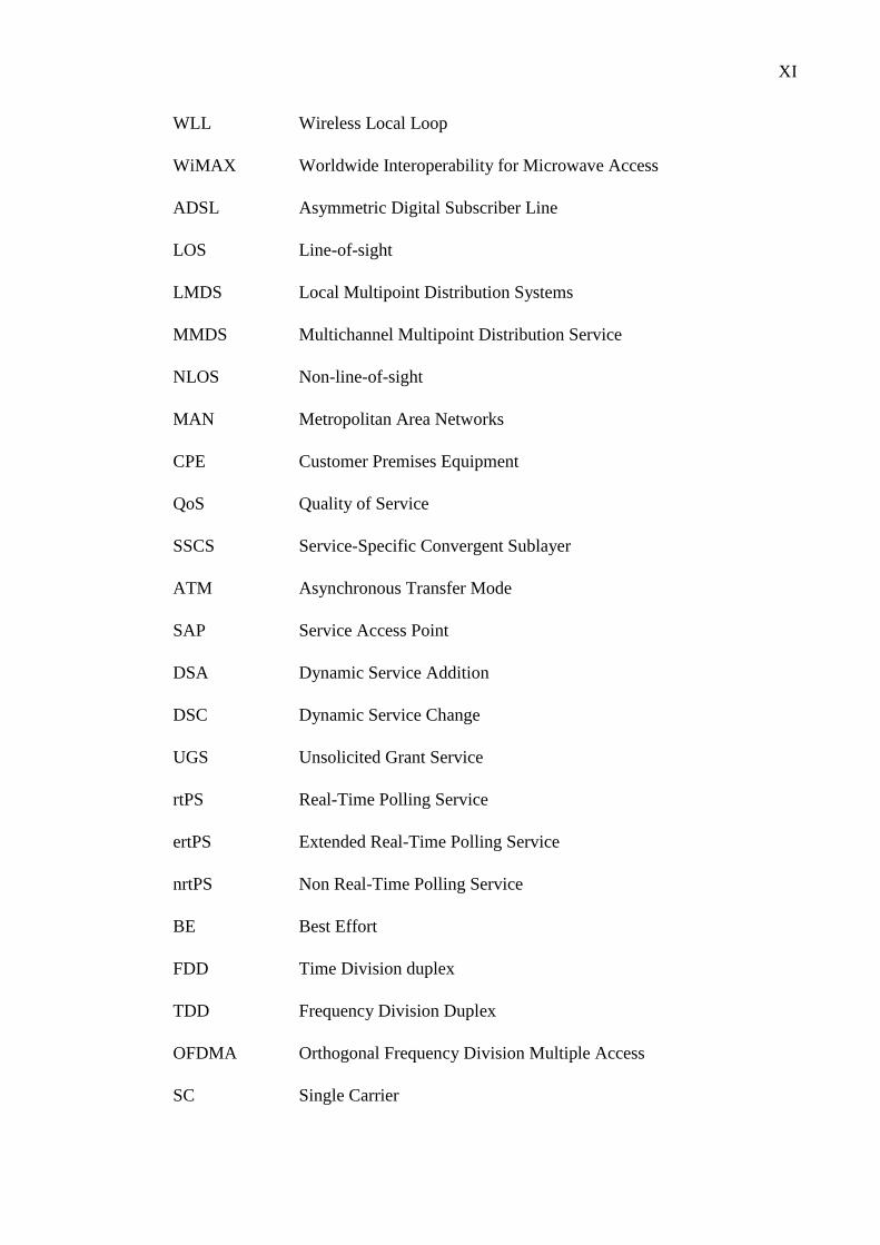
WLL Wireless Local Loop
WiMAX Worldwide Interoperability for Microwave Access
ADSL Asymmetric Digital Subscriber Line
LOS Line-of-sight
LMDS Local Multipoint Distribution Systems
MMDS Multichannel Multipoint Distribution Service
NLOS Non-line-of-sight
MAN Metropolitan Area Networks
CPE Customer Premises Equipment
QoS Quality of Service
SSCS Service-Specific Convergent Sublayer
ATM Asynchronous Transfer Mode
SAP Service Access Point
DSA Dynamic Service Addition
DSC Dynamic Service Change
UGS Unsolicited Grant Service
rtPS Real-Time Polling Service
ertPS Extended Real-Time Polling Service
nrtPS Non Real-Time Polling Service
BE Best Effort
FDD Time Division duplex
TDD Frequency Division Duplex
OFDMA Orthogonal Frequency Division Multiple Access
SC Single Carrier
XII
ARQ Automatic Repeat Request
HUMAN High Speed Unlicensed Metropolitan Area Network
TOA Time of Arrival
TDOA Time Difference of Arrival
RTOF Round-Trip Time of Flight
RTT Round-Trip Time
AOA Angle of Arrival
Cell-ID Cell identifier
RSS Received Signal Strength
NN Nearest Neighbor
FP Fingerprinting
PL Pathloss
PDF Probability Density Function
LS Least Squares
MMSE Minimum Mean Square Error
POCS Projection Onto Convex Sets
WSN Wireless Sensor Network
SDP Semi-Definite Programming
MDS Miltidimensional Scaling
MLE Maximum Likelihood Estimation
P2P Peer to Peer
NBP Non-Parametric Belief Propagation
BP Belief Propagation
SPA Sum-Product Algorithm

XIII
SMC Sequential Monte Carlo
LSE Least Squares Estimation
1
1 Introduction
The new technology developments have increased the use of mobile phones in our
lives. As time has passed, the hardware characteristics of phones have become more and
more complex allowing the introduction of a wide range of services, and also, a new
concept for mobile phones has been introduced, nowadays known as smartphones.
At the beginning of their introduction to the market, the typical use of mobile phones
was to make voice calls and send SMSs, but today phones can even be used for social
network applications, e-mails, uploading pictures online, retrieving location-based
information, etc. This fact has allowed phones to turn into advanced social-networking
tools, involving an increasing need to offer the consumers/users new services. All this
implies an increment in research and development efforts towards more powerful and
more versatile mobile phone engines.
Location information and location-based service have recently appeared in the new
generation of smartphones, and it is now becoming a hot topic in society, industry and
research. This new service has opened a new business market with a lot of power, which
encompass emergency services, security, monitoring, tracking, logistics, etc. This fact has
driven the manufacturers to build mobile handsets with the necessary embedded
technology to provide location information with a high level of accuracy anywhere and
anytime [1].
At the moment, the most popular commercial localization solution is the Global
Positioning System (GPS), which is embedded in the current hardware designs of
smartphones. However, it has to be pointed out that the GPS has several drawbacks, such
as the lack of satellite signals in adverse environments, such as indoors and heavy urban
scenarios, and its high battery energy consumption. From the point of view of signal
availability, the signal blocking and multipath condition make it a difficult, if not
impossible, task to receive the satellite signals in outdoors urban canyons, indoor
environments and underground [1] [2], which actually represent the greatest interest of
service providers.
In order to solve the localization problem for any environment, several lines of
research have been created, which most of them focus on solving the localization problem
in outdoor scenarios. Nevertheless, new lines focusing on indoor environments
localization have been started in recent years too, whose purpose is to investigate if
cellular and WLAN technologies can overcome the GPS challenges to achieve
localization and navigation in indoor environments.
1. INTRODUCTION 2
Motivation
There are several applications that offer the users outdoor localization services with
sufficient accuracy, however, the number of indoor applications has been increasing in
the past years. Moreover, the demand to integrate outdoor and indoor localization in the
same mobile application has grown, for that reason it is necessary to improve the methods
used to perform indoor localization. To this end, several companies have started working
together as is the case of In-Location Alliance formed in August 2012 [3].
Researchers have studied the concept of cooperative localization by utilizing the
additional information obtained from short-range links in order to enhance the location
estimation accuracy in forthcoming cellular systems [1], and this method can easily be
applied to indoor scenarios with a high level of accuracy. Moreover, the concept of
Signals of Opportunity1 (SoO) for outdoor positioning appears when the reception of GPS
signals becomes unreliable [4]. The idea of cooperation between two or more
communication links improves the position estimation if the Base Stations (BS) of each
SoO is well known.
In [5] there are some experimental results introduced that were obtained in a real
indoor scenario with a Wireless Local Area Network (WLAN) infrastructure, and they
demonstrate the accuracy enhancement of localization considering also the information
obtained from communication links between mobile stations (MS), i.e., MS-MS links.
The results denote the better performance of cooperative schemes against non-
cooperative schemes. On the other hand, [6] evaluates that the position error is directly
proportional to the MS present in the scenario, and the metric used to evaluate it is the
Average Root Mean Square Error (RMSE).
Another example is the research from [7] which addresses the human effects, such
as hand-grip and mobile orientation when held in the hand, while performing Received
Signal Strengths (RSS) for localization applications. Additionally, [7] highlights the
importance of mitigating these error sources in order to enhance the positioning accuracy.
In the context of Wireless Sensor Networks (WSN) [8], the need to use low-
computational load algorithms in limited hardware structures, i.e., wireless sensors, is
important. Here RSS-based approaches are the best choice but one of the major issues is
to find the best model to characterize the radio channel in order to obtain the inter-node
distance estimates. Both methods, non-cooperative and cooperative, are simulated in
different scenarios and, subsequently, their results are evaluated and discussed,
concluding that the cooperation presents better performance in user localization and
tracking.
1 Signals of opportunity are those signals that are not originally intended (designed) for positioning but
they are freely available all the time and everywhere (within a certain range, of course) [4]
1. INTRODUCTION 3
The aforementioned studies indicate the viability of using WLANs for indoor
positioning applications. Bearing this in mind, the objective of this thesis is to study the
impact of WLANs combined with Cooperative and Non-Cooperative methods. By
comparing to existing methods in the open literature, we try to reduce the complexity of
the solution in order to achieve easy-to-implement solutions, in other words, the solutions
adopted are feasible solutions for user devices. For that reason, RSS approach is selected.
With the purpose to reduce the uncertainty in the accuracy, it is necessary to realize a
reliable estimation of the wireless channel conditions, such as shadowing standard
deviation (σ2) and path loss exponent (n).
Author’s contributions
The main objective has been to investigate the accuracy limits of various RSS-based
localization methods used in cooperative and non-cooperative positioning algorithms.
The algorithms are compared by simulating some possible environments and analyzing
the errors that they perform during the estimation stage. The authors has contributed to
the followings:
Literature review of indoor localization methods nowadays, such as cooperative
and non-cooperative localization methods
Implementation (in Matlab) of an indoor WLAN localization simulator using both
fingerprinting and path-loss approach in a two dimensional scenario
Analysis of the impact of various modeling parameters (such as AP variability
and shadowing effects) on the positioning accuracy
Comparative analysis of the non-cooperative WLAN positioning with cooperative
WLAN positioning based on the built simulator
Testing of the algorithms with real-field measurement data available in the
research group (measurements done in a university building in Tampere)
Outline
The organization of the thesis is described below in more detail.
Chapter 2 presents an overview of the current Wireless Network standards and their
classification from the point of view of radius coverage, such as WPAN, WLAN, WMAN
and WWAN. In this work we pays special attention to the IEEE 802.11 standard for
WLAN, which is widely used nowadays. Also, some characteristics from the physical
layer are described.
Chapter 3 addresses to non-cooperative localization methods. Two approaches are
studied in more detail, namely Fingerprinting and Probabilistic/Path-Loss approaches. In
the Training/Offline phase, we will describe how data measurements can be done and
1. INTRODUCTION 4
how to use these measurements to estimate the channel parameters. Subsequently, in the
estimation phase we introduce the most common algorithms applied in both approaches.
Finally, simulation results are presented to compare the performance between
Fingerprinting and Path-Loss.
Chapter 4 presents an overview of the generic cooperative methods. Our basic
purpose is to propose and develop approaches based in cooperative methodology.
Chapter 5 demonstrates to the reader the comparison between both, cooperative and
non-cooperative methods and the approaches simulated, studying the accuracy effect
achieved from each of them. This comparison is carried out showing the simulation
results in merit metrics, such as the cost functions criteria, the RMSE and the Average
RMSE.
Chapter 6 concludes with a discussion of the obtained results and, also, some
suggestions for future work are presented.
5
2 Wireless Networks
Over the past five years, the wireless technology is permeating almost all the business
fields, such as, communication, medicine, automation, security, etc. As a result, wireless
technologies are one of the best options for networking applications, where free
movement is needed. If users must be connected to a network by physical cables, their
movement is dramatically reduced [9].
The remarkable advantages of wireless networks are [9]:
Mobility, wireless network users can connect to existing networks and are then
allowed to roam freely. These networks allow different levels of mobility:
o No mobility, the receiver has to be in a fixed position.
o Mobility in the range of the wireless transmitter.
o Mobility between different wireless transmitters.
Flexibility, the wireless infrastructure does not need to be reconfigured to add new
users, which can be translated into independence of the number of users to be
connected. This is an important attribute for service providers. Thanks to the
flexibility, a new market that many equipment vendors and service providers have
been chasing is the Wi-Fi Hot-Spots. The best way to increase the implicit benefits
of attracting more customers to public gathering spots is by offering internet
access. A point in case is a coffeehouse, shopping center, etc.
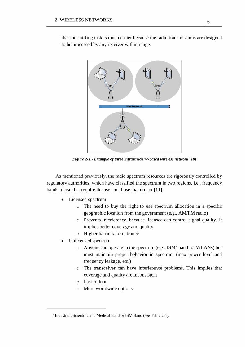
Although these networks have advantages, today they need to have a fixed
infrastructure. Infrastructure networks not only provide access to other networks, but also
include forwarding functions, medium access control etc. From the Figure 2-1, we can
observe that in these infrastructure-based wireless networks, communication typically
takes place only between the wireless nodes and the access point, but not directly between
the wireless nodes [10].
Moreover, there are implicit disadvantages in the wireless networks[9]:
Transmission speed is typically an order of magnitude lower than wired networks,
e.g., Gigabit Ethernet (IEEE 802.3z) against from 450 Mbps of IEEE 802.11n.
The use of radio spectrum resources, which is rigorously controlled by regulatory
authorities through licensing processes. Wireless devices are constrained to
operate in a certain frequency band. Each band has an associated bandwidth,
which is simply the amount of frequency space in the band.
Security on wireless networks is often a critical concern, because the signal
transmissions are available to anyone within the range of the transmitter. It implies
2. WIRELESS NETWORKS 6
that the sniffing task is much easier because the radio transmissions are designed
to be processed by any receiver within range.
Figure 2-1.- Example of three infrastructure-based wireless network [10]
As mentioned previously, the radio spectrum resources are rigorously controlled by
regulatory authorities, which have classified the spectrum in two regions, i.e., frequency
bands: those that require license and those that do not [11].
Licensed spectrum
o The need to buy the right to use spectrum allocation in a specific
geographic location from the government (e.g., AM/FM radio)
o Prevents interference, because licensee can control signal quality. It
implies better coverage and quality
o Higher barriers for entrance
Unlicensed spectrum
o Anyone can operate in the spectrum (e.g., ISM2 band for WLANs) but
must maintain proper behavior in spectrum (max power level and
frequency leakage, etc.)
o The transceiver can have interference problems. This implies that
coverage and quality are inconsistent
o Fast rollout
o More worldwide options
2 Industrial, Scientific and Medical Band or ISM Band (see Table 2-1).
2. WIRELESS NETWORKS 7
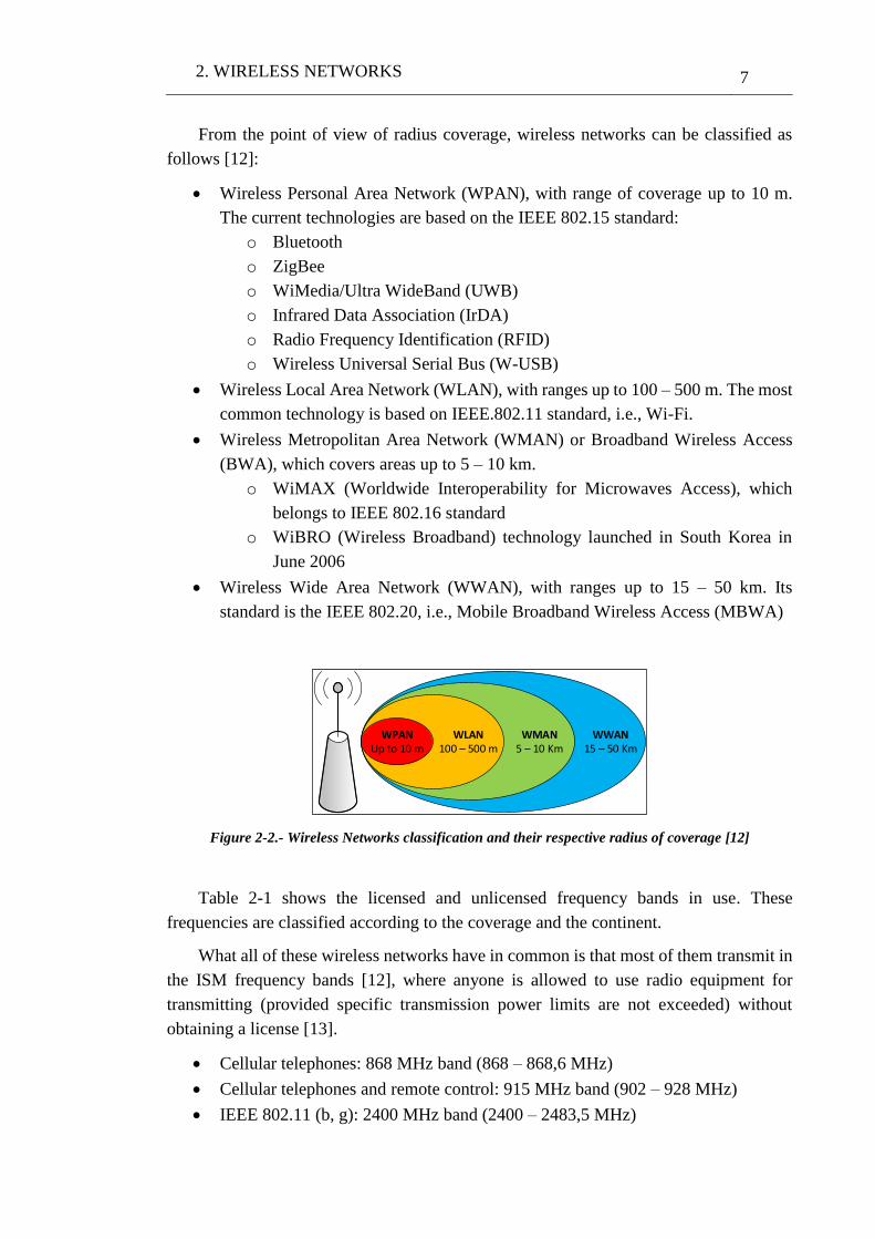
From the point of view of radius coverage, wireless networks can be classified as
follows [12]:
Wireless Personal Area Network (WPAN), with range of coverage up to 10 m.
The current technologies are based on the IEEE 802.15 standard:
o Bluetooth
o ZigBee
o WiMedia/Ultra WideBand (UWB)
o Infrared Data Association (IrDA)
o Radio Frequency Identification (RFID)
o Wireless Universal Serial Bus (W-USB)
Wireless Local Area Network (WLAN), with ranges up to 100 – 500 m. The most
common technology is based on IEEE.802.11 standard, i.e., Wi-Fi.
Wireless Metropolitan Area Network (WMAN) or Broadband Wireless Access
(BWA), which covers areas up to 5 – 10 km.
o WiMAX (Worldwide Interoperability for Microwaves Access), which
belongs to IEEE 802.16 standard
o WiBRO (Wireless Broadband) technology launched in South Korea in
June 2006
Wireless Wide Area Network (WWAN), with ranges up to 15 – 50 km. Its
standard is the IEEE 802.20, i.e., Mobile Broadband Wireless Access (MBWA)
Figure 2-2.- Wireless Networks classification and their respective radius of coverage [12]
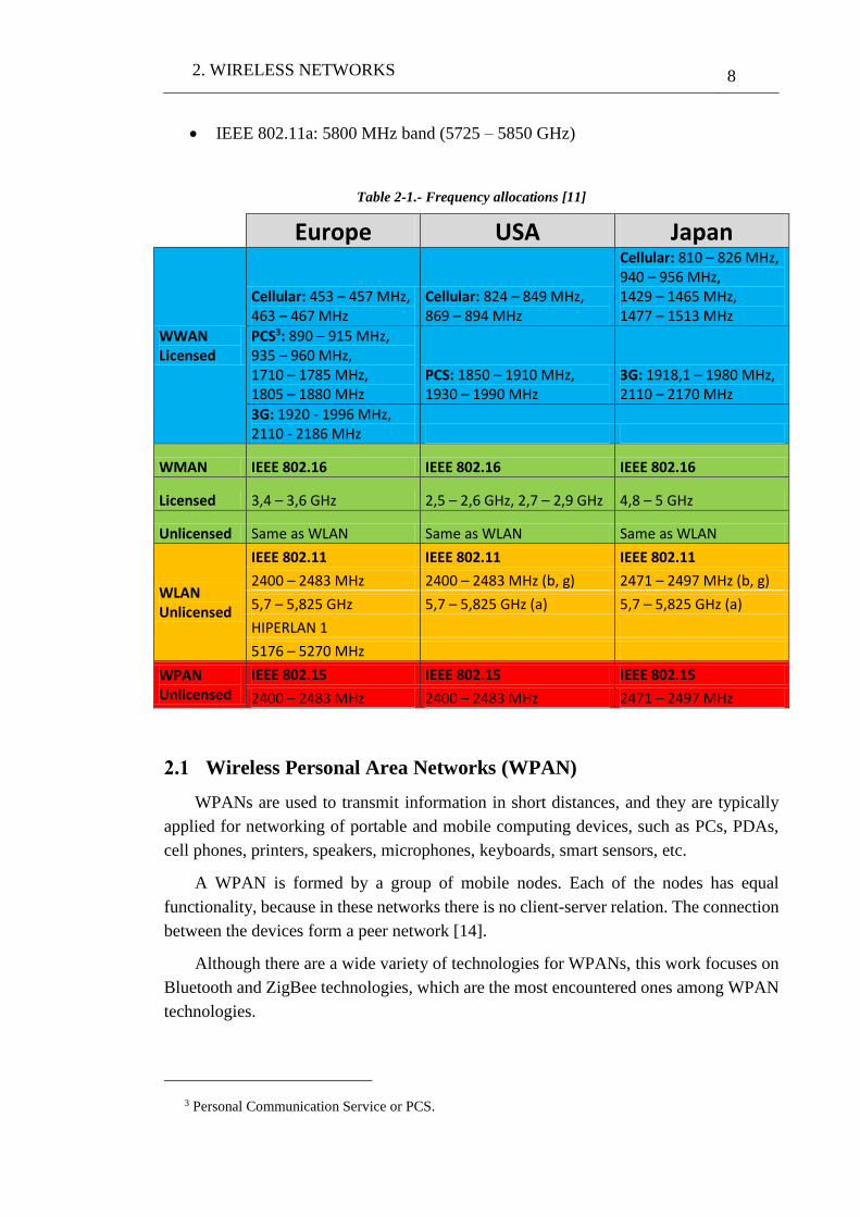
Table 2-1 shows the licensed and unlicensed frequency bands in use. These
frequencies are classified according to the coverage and the continent.
What all of these wireless networks have in common is that most of them transmit in
the ISM frequency bands [12], where anyone is allowed to use radio equipment for
transmitting (provided specific transmission power limits are not exceeded) without
obtaining a license [13].
Cellular telephones: 868 MHz band (868 – 868,6 MHz)
Cellular telephones and remote control: 915 MHz band (902 – 928 MHz)
IEEE 802.11 (b, g): 2400 MHz band (2400 – 2483,5 MHz)
WPANUp to 10 m
WLAN100 – 500 m
WMAN5 – 10 Km
WWAN15 – 50 Km
2. WIRELESS NETWORKS 8
IEEE 802.11a: 5800 MHz band (5725 – 5850 GHz)
Table 2-1.- Frequency allocations [11]
Europe USA Japan
WWAN Licensed
Cellular: 453 – 457 MHz, 463 – 467 MHz
Cellular: 824 – 849 MHz, 869 – 894 MHz
Cellular: 810 – 826 MHz, 940 – 956 MHz, 1429 – 1465 MHz, 1477 – 1513 MHz
PCS3: 890 – 915 MHz, 935 – 960 MHz, 1710 – 1785 MHz, 1805 – 1880 MHz
PCS: 1850 – 1910 MHz, 1930 – 1990 MHz
3G: 1918,1 – 1980 MHz, 2110 – 2170 MHz
3G: 1920 - 1996 MHz, 2110 - 2186 MHz
WMAN IEEE 802.16 IEEE 802.16 IEEE 802.16
Licensed 3,4 – 3,6 GHz 2,5 – 2,6 GHz, 2,7 – 2,9 GHz 4,8 – 5 GHz
Unlicensed Same as WLAN Same as WLAN Same as WLAN
WLAN Unlicensed
IEEE 802.11 IEEE 802.11 IEEE 802.11
2400 – 2483 MHz 2400 – 2483 MHz (b, g) 2471 – 2497 MHz (b, g)
5,7 – 5,825 GHz 5,7 – 5,825 GHz (a) 5,7 – 5,825 GHz (a)
HIPERLAN 1
5176 – 5270 MHz
WPAN Unlicensed
IEEE 802.15 IEEE 802.15 IEEE 802.15
2400 – 2483 MHz 2400 – 2483 MHz 2471 – 2497 MHz
Wireless Personal Area Networks (WPAN)
WPANs are used to transmit information in short distances, and they are typically
applied for networking of portable and mobile computing devices, such as PCs, PDAs,
cell phones, printers, speakers, microphones, keyboards, smart sensors, etc.
A WPAN is formed by a group of mobile nodes. Each of the nodes has equal
functionality, because in these networks there is no client-server relation. The connection
between the devices form a peer network [14].
Although there are a wide variety of technologies for WPANs, this work focuses on
Bluetooth and ZigBee technologies, which are the most encountered ones among WPAN
technologies.
3 Personal Communication Service or PCS.
2. WIRELESS NETWORKS 9
2.1.1 Bluetooth
Bluetooth is a short distance radio-based network technology used to transmit voice
and data. It was originally developed for cable replacement in Personal Area Networking
(PAN) to operate all over the world, and, at the moment, it is the most popular technology
designed for short range [15].
Bluetooth is an inexpensive personal area Ad Hoc4 network operating in unlicensed
bands and owned by the user [15]. Its aims are so-called Ad Hoc piconets, which are local
area networks with a very limited coverage and without the need for an infrastructure.
This technology allows connecting different small devices in close proximity without
expensive wiring and without the need for a wireless infrastructure. Its commercial
representation is a low-cost single-chip, based on radio wireless network technology [12].
Piconets are established dynamically and automatically and each Bluetooth device
can enter and leave the network within the radio proximity [13]. A piconet is defined by
a master device, which controls the hopping pattern and, also, controls the transmission
within its piconet [16]. All devices using the same hopping sequence with the same phase
form a Bluetooth piconet, which means that each piconet has a unique hopping pattern
[12].
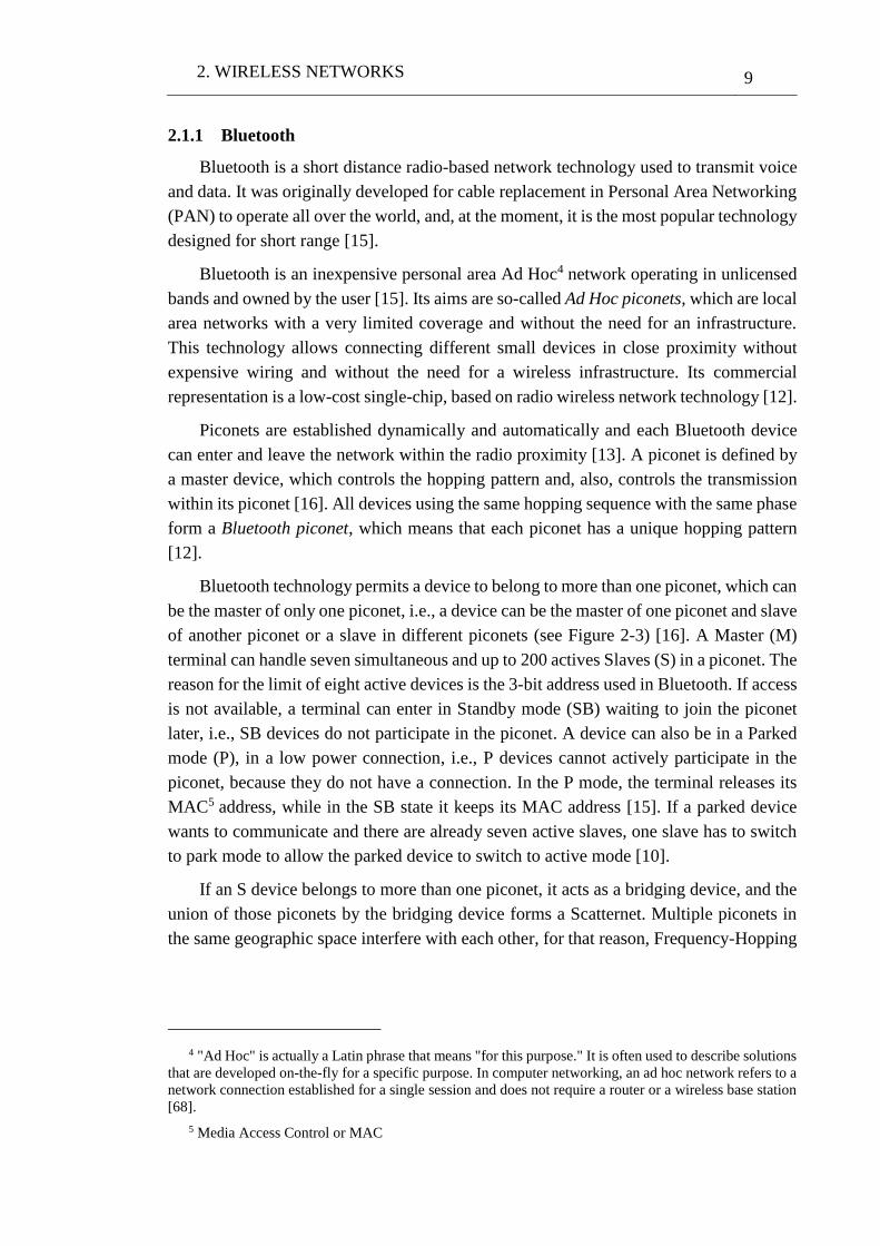
Bluetooth technology permits a device to belong to more than one piconet, which can
be the master of only one piconet, i.e., a device can be the master of one piconet and slave
of another piconet or a slave in different piconets (see Figure 2-3) [16]. A Master (M)
terminal can handle seven simultaneous and up to 200 actives Slaves (S) in a piconet. The
reason for the limit of eight active devices is the 3-bit address used in Bluetooth. If access
is not available, a terminal can enter in Standby mode (SB) waiting to join the piconet
later, i.e., SB devices do not participate in the piconet. A device can also be in a Parked
mode (P), in a low power connection, i.e., P devices cannot actively participate in the
piconet, because they do not have a connection. In the P mode, the terminal releases its
MAC5 address, while in the SB state it keeps its MAC address [15]. If a parked device
wants to communicate and there are already seven active slaves, one slave has to switch
to park mode to allow the parked device to switch to active mode [10].
If an S device belongs to more than one piconet, it acts as a bridging device, and the
union of those piconets by the bridging device forms a Scatternet. Multiple piconets in
the same geographic space interfere with each other, for that reason, Frequency-Hopping
4 "Ad Hoc" is actually a Latin phrase that means "for this purpose." It is often used to describe solutions
that are developed on-the-fly for a specific purpose. In computer networking, an ad hoc network refers to a
network connection established for a single session and does not require a router or a wireless base station
[68].
5 Media Access Control or MAC
2. WIRELESS NETWORKS 10
Spread Spectrum (FHSS) scheme is used so that multiple piconets can coexist in same
space [16].
Figure 2-3.- Bluetooth scatternet [10]
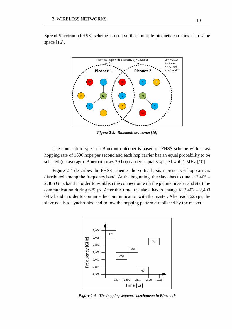
The connection type in a Bluetooth piconet is based on FHSS scheme with a fast
hopping rate of 1600 hops per second and each hop carrier has an equal probability to be
selected (on average). Bluetooth uses 79 hop carriers equally spaced with 1 MHz [10].
Figure 2-4 describes the FHSS scheme, the vertical axis represents 6 hop carriers
distributed among the frequency band. At the beginning, the slave has to tune at 2,405 –
2,406 GHz band in order to establish the connection with the piconet master and start the
communication during 625 µs. After this time, the slave has to change to 2,402 – 2,403
GHz band in order to continue the communication with the master. After each 625 µs, the
slave needs to synchronize and follow the hopping pattern established by the master.
Figure 2-4.- The hopping sequence mechanism in Bluetooth
M
S
S
S
Piconet-1
P
SBP
M
S P
S
Piconet-2
SBSB
P
M = MasterS = SlaveP = ParkedSB = Standby
Piconets (each with a capacity of < 1 Mbps)
1st
2nd
3rd
4th
5th
2,406
2,405
2,404
2,403
2,402
2,401
2,400
Fre
qu
ency
[G
Hz]
625 1250 1875 2500 3125
Time [µs]
2. WIRELESS NETWORKS 11
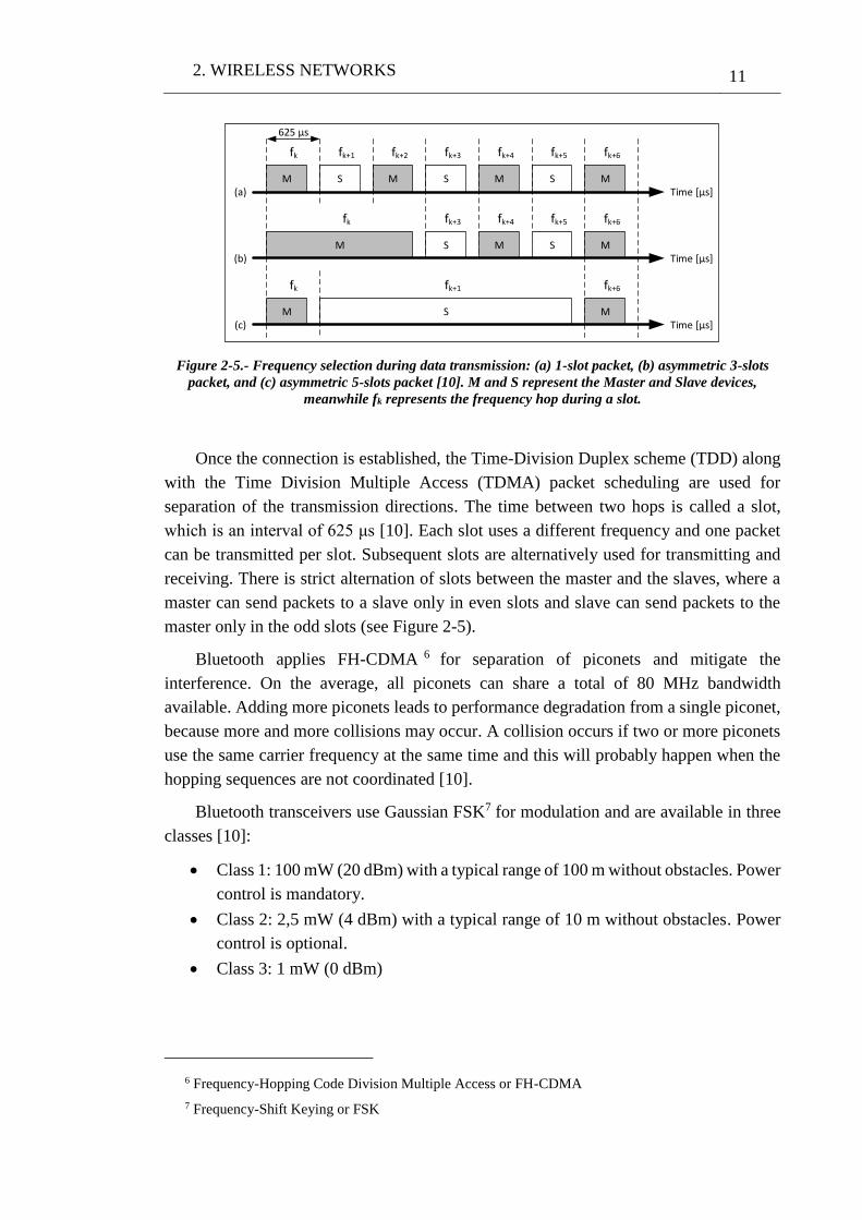
Figure 2-5.- Frequency selection during data transmission: (a) 1-slot packet, (b) asymmetric 3-slots
packet, and (c) asymmetric 5-slots packet [10]. M and S represent the Master and Slave devices,
meanwhile fk represents the frequency hop during a slot.
Once the connection is established, the Time-Division Duplex scheme (TDD) along
with the Time Division Multiple Access (TDMA) packet scheduling are used for
separation of the transmission directions. The time between two hops is called a slot,
which is an interval of 625 μs [10]. Each slot uses a different frequency and one packet
can be transmitted per slot. Subsequent slots are alternatively used for transmitting and
receiving. There is strict alternation of slots between the master and the slaves, where a
master can send packets to a slave only in even slots and slave can send packets to the
master only in the odd slots (see Figure 2-5).
Bluetooth applies FH-CDMA 6 for separation of piconets and mitigate the
interference. On the average, all piconets can share a total of 80 MHz bandwidth
available. Adding more piconets leads to performance degradation from a single piconet,
because more and more collisions may occur. A collision occurs if two or more piconets
use the same carrier frequency at the same time and this will probably happen when the
hopping sequences are not coordinated [10].
Bluetooth transceivers use Gaussian FSK7 for modulation and are available in three
classes [10]:
Class 1: 100 mW (20 dBm) with a typical range of 100 m without obstacles. Power
control is mandatory.
Class 2: 2,5 mW (4 dBm) with a typical range of 10 m without obstacles. Power
control is optional.
Class 3: 1 mW (0 dBm)
6 Frequency-Hopping Code Division Multiple Access or FH-CDMA
7 Frequency-Shift Keying or FSK
SM M S M S MTime [µs]
625 µs
fk fk+1 fk+2 fk+3 fk+4 fk+5 fk+6
M
fk
S M S M
fk+3 fk+4 fk+5 fk+6
M S M
fk fk+1 fk+6
Time [µs]
Time [µs]
(a)
(b)
(c)
2. WIRELESS NETWORKS 12
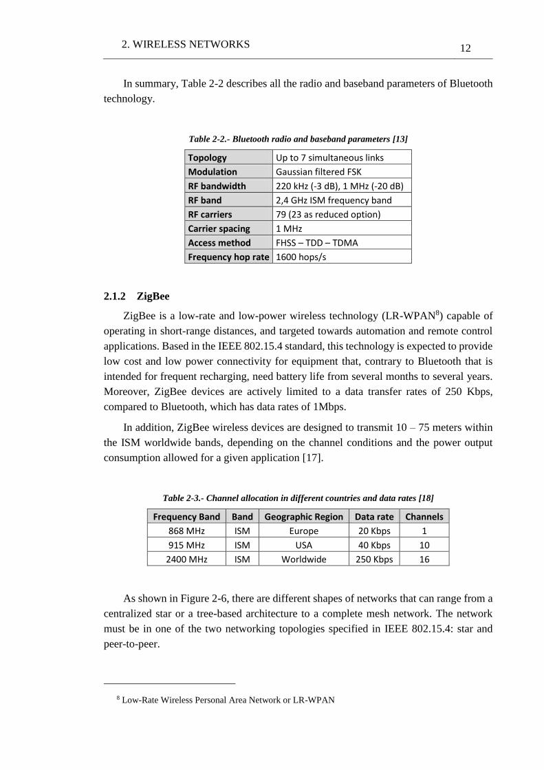
In summary, Table 2-2 describes all the radio and baseband parameters of Bluetooth
technology.
Table 2-2.- Bluetooth radio and baseband parameters [13]
Topology Up to 7 simultaneous links
Modulation Gaussian filtered FSK
RF bandwidth 220 kHz (-3 dB), 1 MHz (-20 dB)
RF band 2,4 GHz ISM frequency band
RF carriers 79 (23 as reduced option)
Carrier spacing 1 MHz
Access method FHSS – TDD – TDMA
Frequency hop rate 1600 hops/s
2.1.2 ZigBee
ZigBee is a low-rate and low-power wireless technology (LR-WPAN8) capable of
operating in short-range distances, and targeted towards automation and remote control
applications. Based in the IEEE 802.15.4 standard, this technology is expected to provide
low cost and low power connectivity for equipment that, contrary to Bluetooth that is
intended for frequent recharging, need battery life from several months to several years.
Moreover, ZigBee devices are actively limited to a data transfer rates of 250 Kbps,
compared to Bluetooth, which has data rates of 1Mbps.
In addition, ZigBee wireless devices are designed to transmit 10 – 75 meters within
the ISM worldwide bands, depending on the channel conditions and the power output
consumption allowed for a given application [17].
Table 2-3.- Channel allocation in different countries and data rates [18]
Frequency Band Band Geographic Region Data rate Channels
868 MHz ISM Europe 20 Kbps 1
915 MHz ISM USA 40 Kbps 10
2400 MHz ISM Worldwide 250 Kbps 16
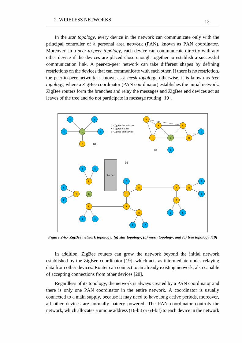
As shown in Figure 2-6, there are different shapes of networks that can range from a
centralized star or a tree-based architecture to a complete mesh network. The network
must be in one of the two networking topologies specified in IEEE 802.15.4: star and
peer-to-peer.
8 Low-Rate Wireless Personal Area Network or LR-WPAN
2. WIRELESS NETWORKS 13
In the star topology, every device in the network can communicate only with the
principal controller of a personal area network (PAN), known as PAN coordinator.
Moreover, in a peer-to-peer topology, each device can communicate directly with any
other device if the devices are placed close enough together to establish a successful
communication link. A peer-to-peer network can take different shapes by defining
restrictions on the devices that can communicate with each other. If there is no restriction,
the peer-to-peer network is known as a mesh topology, otherwise, it is known as tree
topology, where a ZigBee coordinator (PAN coordinator) establishes the initial network.
ZigBee routers form the branches and relay the messages and ZigBee end devices act as
leaves of the tree and do not participate in message routing [19].
Figure 2-6.- ZigBee network topology: (a) star topology, (b) mesh topology, and (c) tree topology [19]
In addition, ZigBee routers can grow the network beyond the initial network
established by the ZigBee coordinator [19], which acts as intermediate nodes relaying
data from other devices. Router can connect to an already existing network, also capable
of accepting connections from other devices [20].
Regardless of its topology, the network is always created by a PAN coordinator and
there is only one PAN coordinator in the entire network. A coordinator is usually
connected to a main supply, because it may need to have long active periods, moreover,
all other devices are normally battery powered. The PAN coordinator controls the
network, which allocates a unique address (16-bit or 64-bit) to each device in the network
E
E C
E
E
R
R
R C
R
R
E
R
E
C = ZigBee CoordinatorR = ZigBee RouterE = ZigBee End Device
(a)
(b)
C
Barrier
E
R
R
E E
R
E
E
R
E E
R
R
E E
R
R
E E
E
E
R
R
(c)
2. WIRELESS NETWORKS 14
and selects a unique PAN identifier for the network. This PAN identifier allows the
devices within a network to use the 16-bit short-addressing method and still be able to
communicate with other devices across independent networks. Also, the coordinator is
responsible of initiating the network and selecting the network parameters such as radio
frequency channel, routing the messages throughout the network, and terminating the
network [19].
On the other hand, the End Devices can be low-power/battery-powered devices,
which can collect information from sensors and switches. They have sufficient
functionality to talk to their parents (either the coordinator or a router) and cannot relay
data from other devices. This reduced functionality can lead to reduce both economic
costs and energy consumption. These devices do not have to be in the online mode the
whole time, while the devices belonging to the other two categories have to, this means
reducing the power consumption and increasing their battery life [20].
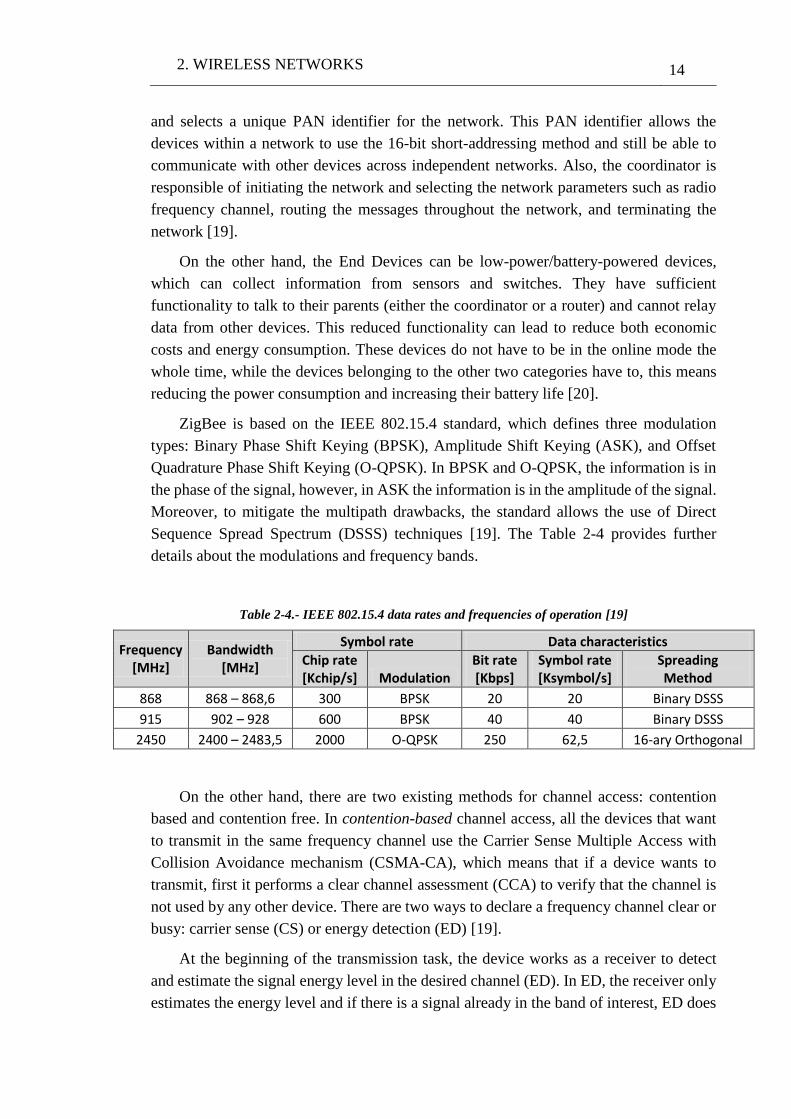
ZigBee is based on the IEEE 802.15.4 standard, which defines three modulation
types: Binary Phase Shift Keying (BPSK), Amplitude Shift Keying (ASK), and Offset
Quadrature Phase Shift Keying (O-QPSK). In BPSK and O-QPSK, the information is in
the phase of the signal, however, in ASK the information is in the amplitude of the signal.
Moreover, to mitigate the multipath drawbacks, the standard allows the use of Direct
Sequence Spread Spectrum (DSSS) techniques [19]. The Table 2-4 provides further
details about the modulations and frequency bands.
Table 2-4.- IEEE 802.15.4 data rates and frequencies of operation [19]
Frequency [MHz]
Bandwidth [MHz]
Symbol rate Data characteristics
Chip rate [Kchip/s] Modulation
Bit rate [Kbps]
Symbol rate [Ksymbol/s]
Spreading Method
868 868 – 868,6 300 BPSK 20 20 Binary DSSS
915 902 – 928 600 BPSK 40 40 Binary DSSS
2450 2400 – 2483,5 2000 O-QPSK 250 62,5 16-ary Orthogonal
On the other hand, there are two existing methods for channel access: contention
based and contention free. In contention-based channel access, all the devices that want
to transmit in the same frequency channel use the Carrier Sense Multiple Access with
Collision Avoidance mechanism (CSMA-CA), which means that if a device wants to
transmit, first it performs a clear channel assessment (CCA) to verify that the channel is
not used by any other device. There are two ways to declare a frequency channel clear or
busy: carrier sense (CS) or energy detection (ED) [19].
At the beginning of the transmission task, the device works as a receiver to detect
and estimate the signal energy level in the desired channel (ED). In ED, the receiver only
estimates the energy level and if there is a signal already in the band of interest, ED does
2. WIRELESS NETWORKS 15
not determine the type of the signal, which could be IEEE 802.15.4 signal or not.
However, in CS, the type of the occupying signal is determined and if this signal is an
IEEE 802.15.4 signal, the device will consider the channel to be busy even if the signal
energy is below a user-defined threshold [19].
If the channel is being used, the device backs off for a random period of time and
tries again. The random back-off and retry are repeated until either the channel becomes
clear or the device reaches its user-defined maximum number of retries [19].
Moreover, in the contention-free method, the PAN coordinator dedicates a specific
time slot to a particular device. This is called a guaranteed time slot (GTS), which the
bandwidth for each node operating in this method is guaranteed and they will start
transmitting during that GTS without using the CSMA-CA mechanism [19].
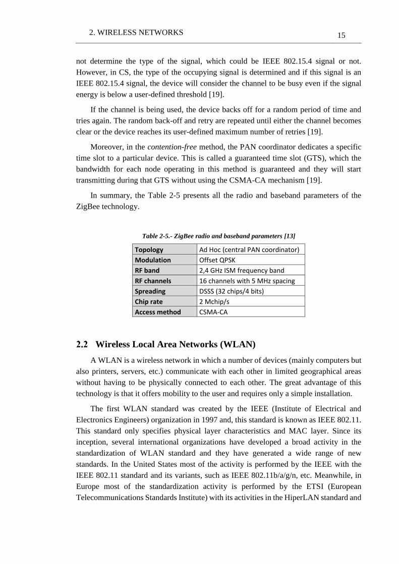
In summary, the Table 2-5 presents all the radio and baseband parameters of the
ZigBee technology.
Table 2-5.- ZigBee radio and baseband parameters [13]
Topology Ad Hoc (central PAN coordinator)
Modulation Offset QPSK
RF band 2,4 GHz ISM frequency band
RF channels 16 channels with 5 MHz spacing
Spreading DSSS (32 chips/4 bits)
Chip rate 2 Mchip/s
Access method CSMA-CA
Wireless Local Area Networks (WLAN)
A WLAN is a wireless network in which a number of devices (mainly computers but
also printers, servers, etc.) communicate with each other in limited geographical areas
without having to be physically connected to each other. The great advantage of this
technology is that it offers mobility to the user and requires only a simple installation.
The first WLAN standard was created by the IEEE (Institute of Electrical and
Electronics Engineers) organization in 1997 and, this standard is known as IEEE 802.11.
This standard only specifies physical layer characteristics and MAC layer. Since its
inception, several international organizations have developed a broad activity in the
standardization of WLAN standard and they have generated a wide range of new
standards. In the United States most of the activity is performed by the IEEE with the
IEEE 802.11 standard and its variants, such as IEEE 802.11b/a/g/n, etc. Meanwhile, in
Europe most of the standardization activity is performed by the ETSI (European
Telecommunications Standards Institute) with its activities in the HiperLAN standard and
2. WIRELESS NETWORKS 16
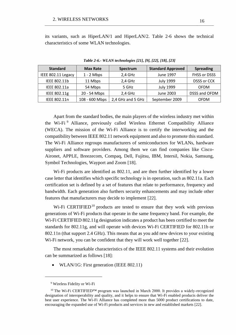
its variants, such as HiperLAN/1 and HiperLAN/2. Table 2-6 shows the technical
characteristics of some WLAN technologies.
Table 2-6.- WLAN technologies [21], [9], [22], [18], [23]
Standard Max Rate Spectrum Standard Approved Spreading
IEEE 802.11 Legacy 1 - 2 Mbps 2,4 GHz June 1997 FHSS or DSSS
IEEE 802.11b 11 Mbps 2,4 GHz July 1999 DSSS or CCK
IEEE 802.11a 54 Mbps 5 GHz July 1999 OFDM
IEEE 802.11g 20 - 54 Mbps 2,4 GHz June 2003 DSSS and OFDM
IEEE 802.11n 108 - 600 Mbps 2,4 GHz and 5 GHz September 2009 OFDM
Apart from the standard bodies, the main players of the wireless industry met within
the Wi-Fi 9 Alliance, previously called Wireless Ethernet Compatibility Alliance
(WECA). The mission of the Wi-Fi Alliance is to certify the interworking and the
compatibility between IEEE 802.11 network equipment and also to promote this standard.
The Wi-Fi Alliance regroups manufacturers of semiconductors for WLANs, hardware
suppliers and software providers. Among them we can find companies like Cisco-
Aironet, APPLE, Breezecom, Compaq, Dell, Fujitsu, IBM, Intersil, Nokia, Samsung,
Symbol Technologies, Wayport and Zoom [18].
Wi-Fi products are identified as 802.11, and are then further identified by a lower
case letter that identifies which specific technology is in operation, such as 802.11a. Each
certification set is defined by a set of features that relate to performance, frequency and
bandwidth. Each generation also furthers security enhancements and may include other
features that manufacturers may decide to implement [22].
Wi-Fi CERTIFIED10 products are tested to ensure that they work with previous
generations of Wi-Fi products that operate in the same frequency band. For example, the
Wi-Fi CERTIFIED 802.11g designation indicates a product has been certified to meet the
standards for 802.11g, and will operate with devices Wi-Fi CERTIFIED for 802.11b or
802.11n (that support 2.4 GHz). This means that as you add new devices to your existing
Wi-Fi network, you can be confident that they will work well together [22].
The most remarkable characteristics of the IEEE 802.11 systems and their evolution
can be summarized as follows [18]:
WLAN/1G: First generation (IEEE 802.11)
9 Wireless Fidelity or Wi-Fi
10 The Wi-Fi CERTIFIED™ program was launched in March 2000. It provides a widely-recognized
designation of interoperability and quality, and it helps to ensure that Wi-Fi enabled products deliver the
best user experience. The Wi-Fi Alliance has completed more than 5000 product certifications to date,
encouraging the expanded use of Wi-Fi products and services in new and established markets [22].
2. WIRELESS NETWORKS 17
o Connectivity of PC terminals (between them or to a fixed LAN)
o Bridge-based APs
o Roaming
o Coexistence with other networks (e.g. WLAN and Ethernet LAN) which
means bridging. Note that there is a small problem in the IEEE 802.11 in
general with respect to bridging where it does not fulfill completely the
bridging rules and is hence non-conformant to the 802 paradigms.
WLAN/2G: Second generation (IEEE 802.11b)
o More effective management of WLAN
o Interworking and interoperability
o Migration starting from the first generation
WLAN/3G: Third generation (802.11a/g)
o High throughput
o Design of networks more open and integrated
o Conformity to the IEEE 802.11a/g standard
o Minimization of antenna sizes
o Improvement of receiver’s sensitivities
WLAN/4G: Fourth generation (IEEE 802.11n)
o Very high throughput
o Long distances at high data rates (equivalent to IEEE 802.11b at 500
Mbps)
o Use of robust technologies, e.g., multiple-input multiple-output (MIMO)
and space time coding
Although there is a wide variety of technologies for IEEE 802.11, this work focuses
on IEEE 802.11b/a/g/n technologies, which are the most encountered ones among WLAN
technologies.
2.2.1 IEEE 802.11
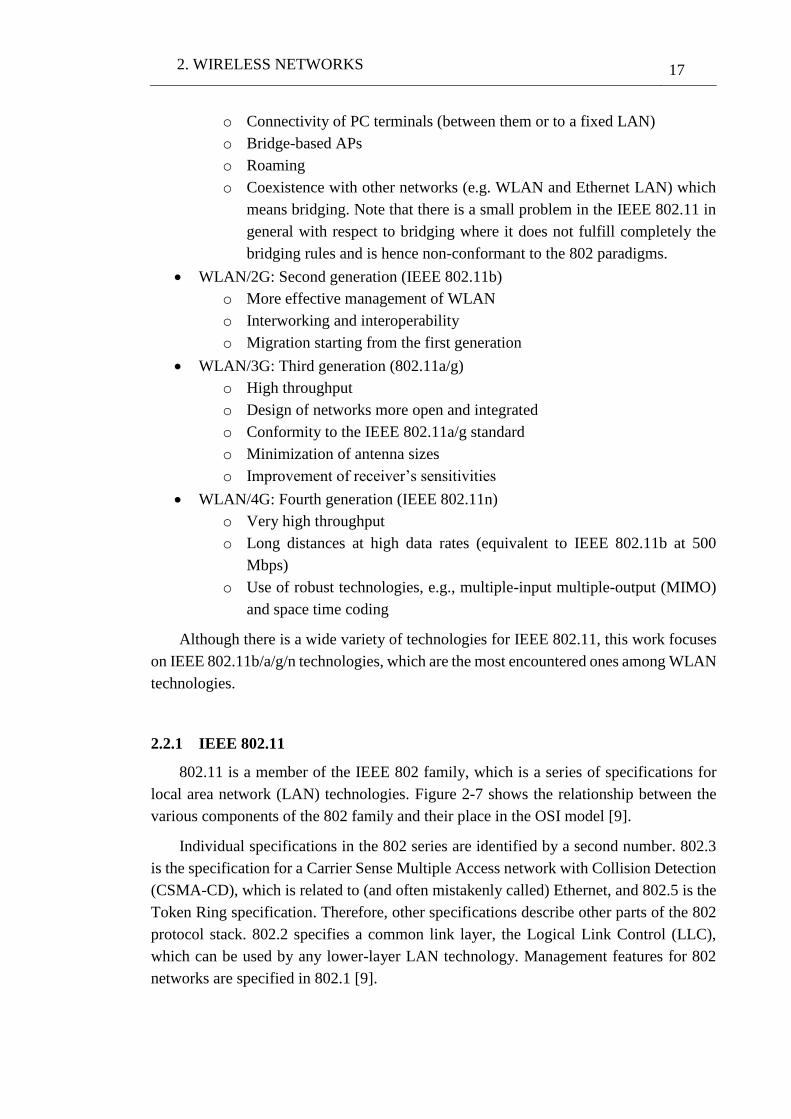
802.11 is a member of the IEEE 802 family, which is a series of specifications for
local area network (LAN) technologies. Figure 2-7 shows the relationship between the
various components of the 802 family and their place in the OSI model [9].
Individual specifications in the 802 series are identified by a second number. 802.3
is the specification for a Carrier Sense Multiple Access network with Collision Detection
(CSMA-CD), which is related to (and often mistakenly called) Ethernet, and 802.5 is the
Token Ring specification. Therefore, other specifications describe other parts of the 802
protocol stack. 802.2 specifies a common link layer, the Logical Link Control (LLC),
which can be used by any lower-layer LAN technology. Management features for 802
networks are specified in 802.1 [9].
2. WIRELESS NETWORKS 18
802Overview and architecture
802.1Management
802.3MAC
802.3PHY
802.5MAC
802.5PHY
802.112,4 GHzInfrared
802.112,4 GHz
DSSS PHY
802.11n2,4 – 5 GHzMIMO PHY
802.11MAC
802.2Logical link control (LLC)
802.4MAC
802.4PHY
CSMA/CD Token Bus Token Ring
Physical layer
MAC sublayer
Data link layerLLC sublayer
802.112,4 GHz
FHSS PHY
802.11a5 GHz
OFDM PHY
802.11b2,4 GHzHR/DSSS
PHY
802.11g2,4 GHz
OFDM PHY
Figure 2-7.- The IEEE 802 family and its relation to the OSI model [9], [18]
802.11 is just another link layer that can use the 802.2/LLC encapsulation. The base
of 802.11 specification includes the 802.11 MAC and two physical layers: a FHSS
physical layer and a DSSS link layer. However, later revisions to 802.11 added additional
physical layers, such as 802.11b and 802.11a. 802.11b specifies a high-rate direct-
sequence layer (HR-DSSS), meanwhile 802.11a describes a physical layer based on
orthogonal frequency division multiplexing (OFDM) [9].
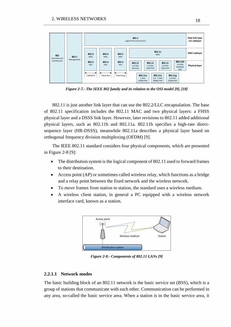
The IEEE 802.11 standard considers four physical components, which are presented
in Figure 2-8 [9]:
The distribution system is the logical component of 802.11 used to forward frames
to their destination.
Access point (AP) or sometimes called wireless relay, which functions as a bridge
and a relay point between the fixed network and the wireless network.
To move frames from station to station, the standard uses a wireless medium.
A wireless client station, in general a PC equipped with a wireless network
interface card, known as a station.
Distribution system
Access point
StationWireless medium
Figure 2-8.- Components of 802.11 LANs [9]
2.2.1.1 Network modes
The basic building block of an 802.11 network is the basic service set (BSS), which is a
group of stations that communicate with each other. Communication can be performed in
any area, so-called the basic service area. When a station is in the basic service area, it
2. WIRELESS NETWORKS 19
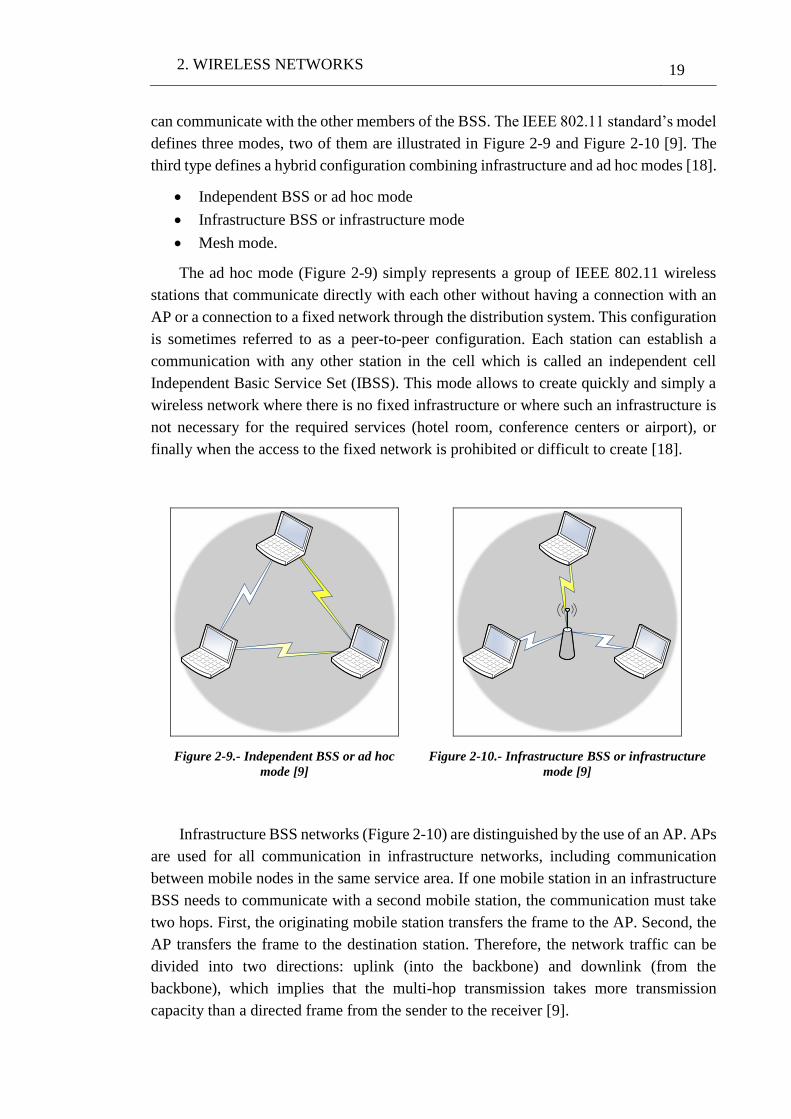
can communicate with the other members of the BSS. The IEEE 802.11 standard’s model
defines three modes, two of them are illustrated in Figure 2-9 and Figure 2-10 [9]. The
third type defines a hybrid configuration combining infrastructure and ad hoc modes [18].
Independent BSS or ad hoc mode
Infrastructure BSS or infrastructure mode
Mesh mode.
The ad hoc mode (Figure 2-9) simply represents a group of IEEE 802.11 wireless
stations that communicate directly with each other without having a connection with an
AP or a connection to a fixed network through the distribution system. This configuration
is sometimes referred to as a peer-to-peer configuration. Each station can establish a
communication with any other station in the cell which is called an independent cell
Independent Basic Service Set (IBSS). This mode allows to create quickly and simply a
wireless network where there is no fixed infrastructure or where such an infrastructure is
not necessary for the required services (hotel room, conference centers or airport), or
finally when the access to the fixed network is prohibited or difficult to create [18].
Figure 2-9.- Independent BSS or ad hoc
mode [9]
Figure 2-10.- Infrastructure BSS or infrastructure
mode [9]
Infrastructure BSS networks (Figure 2-10) are distinguished by the use of an AP. APs
are used for all communication in infrastructure networks, including communication
between mobile nodes in the same service area. If one mobile station in an infrastructure
BSS needs to communicate with a second mobile station, the communication must take
two hops. First, the originating mobile station transfers the frame to the AP. Second, the
AP transfers the frame to the destination station. Therefore, the network traffic can be
divided into two directions: uplink (into the backbone) and downlink (from the
backbone), which implies that the multi-hop transmission takes more transmission
capacity than a directed frame from the sender to the receiver [9].
2. WIRELESS NETWORKS 20
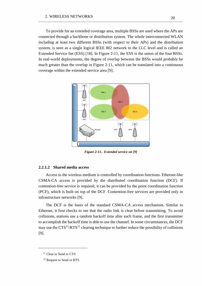
To provide for an extended coverage area, multiple BSSs are used where the APs are
connected through a backbone or distribution system. The whole interconnected WLAN
including at least two different BSSs (with respect to their APs) and the distribution
system, is seen as a single logical IEEE 802 network to the LLC level and is called an
Extended Service Set (ESS) [18]. In Figure 2-11, the ESS is the union of the four BSSs.
In real-world deployments, the degree of overlap between the BSSs would probably be
much greater than the overlap in Figure 2-11, which can be translated into a continuous
coverage within the extended service area [9].
AP1
AP2
BSS 1
BSS 2
BSS 3
BSS 4
AP3 AP4Router
Figure 2-11.- Extended service set [9]
2.2.1.2 Shared media access
Access to the wireless medium is controlled by coordination functions. Ethernet-like
CSMA-CA access is provided by the distributed coordination function (DCF). If
contention-free service is required, it can be provided by the point coordination function
(PCF), which is built on top of the DCF. Contention-free services are provided only in
infrastructure networks [9].
The DCF is the basis of the standard CSMA-CA access mechanism. Similar to
Ethernet, it first checks to see that the radio link is clear before transmitting. To avoid
collisions, stations use a random backoff time after each frame, and the first transmitter
to accomplish the backoff time is able to use the channel. In some circumstances, the DCF
may use the CTS11/RTS12 clearing technique to further reduce the possibility of collisions
[9].
11 Clear to Send or CTS
12 Request to Send or RTS
2. WIRELESS NETWORKS 21
Point coordination provides contention-free services. Special stations called point
coordinators are used to ensure that the medium is provided without contention. Point
coordinators reside in access points, i.e., the PCF is restricted to infrastructure networks.
To gain priority over standard contention-based services, the PCF allows stations to
transmit frames after a shorter interval. The PCF is not widely implemented in current
market products [9].
In order to supervise the network activity, the MAC sublayer works in collaboration
with the physical layer. The physical layer uses CCA algorithm to evaluate the availability
of the channel. To know if the channel is free, the physical layer measures the power
received by antenna called received signal strength indicator (RSSI). The physical layer
thus determines that the channel is free by comparing the RSSI value with a fixed
threshold and transmits thereafter to the MAC layer an indicator of free channel [18].
CSMA/CA protocol is based on [18]:
Sensing the medium thanks to CS procedure (CS carrier sense)
Using interframe space (IFS) timers
Using positive acknowledgements and the collision avoidance approach
Executing backoff algorithm
Using multiple access
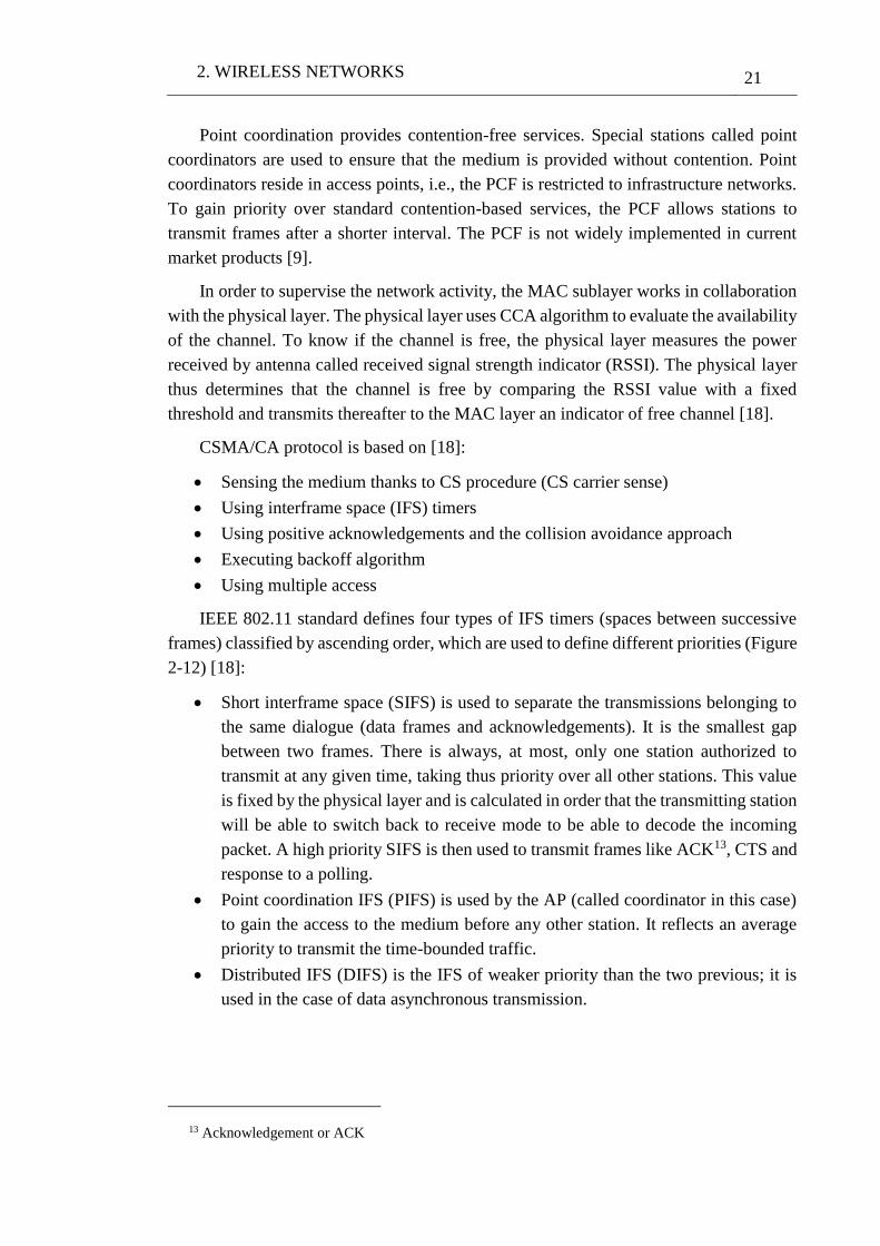
IEEE 802.11 standard defines four types of IFS timers (spaces between successive
frames) classified by ascending order, which are used to define different priorities (Figure
2-12) [18]:
Short interframe space (SIFS) is used to separate the transmissions belonging to
the same dialogue (data frames and acknowledgements). It is the smallest gap
between two frames. There is always, at most, only one station authorized to
transmit at any given time, taking thus priority over all other stations. This value
is fixed by the physical layer and is calculated in order that the transmitting station
will be able to switch back to receive mode to be able to decode the incoming
packet. A high priority SIFS is then used to transmit frames like ACK13, CTS and
response to a polling.
Point coordination IFS (PIFS) is used by the AP (called coordinator in this case)
to gain the access to the medium before any other station. It reflects an average
priority to transmit the time-bounded traffic.
Distributed IFS (DIFS) is the IFS of weaker priority than the two previous; it is
used in the case of data asynchronous transmission.
13 Acknowledgement or ACK
2. WIRELESS NETWORKS 22
Extended IFS (EIFS) is the longest IFS. It is used by a station receiving a packet
which is corrupted by collisions to wait longer than the usual DIFS in order to
avoid future collisions.
ACK
Next frameBackoff windowBusy medium
Busy medium
Time
Time
DIFS SIFS
PIFS
DIFS
Defer accessSelect slot and decrement backoff as long as
medium is idle
Contention window
Slot time
SIFS
Source
Destination
Listen carrier
Figure 2-12.- CSMA-CA basic global mechanism for asynchronous data transmission [18]
When several stations wish to transmit simultaneously, the station wishing to emit
the urgent frames as the acknowledgements will be able to send them in first. Then other
priority frames will be transmitted considered to be like those related to the administration
tasks or the traffic which has delay constraints. Lastly, the least important information
concerning the asynchronous traffic will be transmitted after a longer latency [18].
Medium listening is fulfilled thanks to carrier sensing function in order to determine
if the medium is available. Two types of carrier sensing functions in 802.11 manage this
process: the physical carrier-sensing (PCS) and virtual carrier-sensing (VCS) functions.
If either carrier-sensing function indicates that the medium is busy, the MAC reports this
to higher layers [9]. PCS detects the presence of other stations by analyzing all the frames
on the wireless medium and by detecting the activity on the medium thanks to the relative
energy of its signal compared to the other stations. However, VCS is a procedure for
listening at the MAC layer in the case of a reservation of the medium [18].
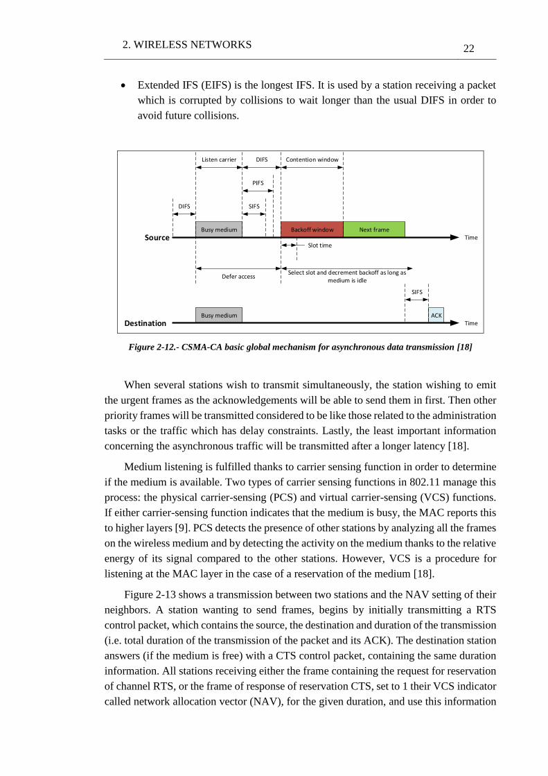
Figure 2-13 shows a transmission between two stations and the NAV setting of their
neighbors. A station wanting to send frames, begins by initially transmitting a RTS
control packet, which contains the source, the destination and duration of the transmission
(i.e. total duration of the transmission of the packet and its ACK). The destination station
answers (if the medium is free) with a CTS control packet, containing the same duration
information. All stations receiving either the frame containing the request for reservation
of channel RTS, or the frame of response of reservation CTS, set to 1 their VCS indicator
called network allocation vector (NAV), for the given duration, and use this information
2. WIRELESS NETWORKS 23
together with the PCS when sensing the medium. If the NAV reaches 0, the VCS function
indicates that the medium is idle. However, if the source does not receive the CTS packet,
it assumes that a collision occurred and will retransmit the RTS packet after a random
waiting period. If the recipient receives the CTS packet correctly, the source emits an
acknowledgement to announce to the recipient that the packet CTS was received. Then
the communication will be able to take place [18].
ACK
Data
Contention window
RTS
NAV (RTS)
Time
Time
SIFS
Source
DestinationCTS
DIFS SIFS
SIFS
NAV (CTS)
NAV (Data)
DIFS
Other station Time
Defer access Backoff
Figure 2-13.- CSMA-CA with RTS-CTS [18]
2.2.1.3 Physical layers variances
Three physical layers (PHY) were standardized in the initial revision of 802.11,
which was published in 1997 [18]:
A radio PHY using an FHSS technique operating in the 2,4 GHz ISM band
A radio PHY using a DSSS technique operating in the 2,4 GHz ISM band
A PHY for the infrared (IR) transmission, which is not widely used, operate in
baseband at wavelength between 850 and 950 nm
The use of spread spectrum techniques increase the performances by minimizing the
harmful effects of the multipath propagation, interferences and noise. In 1999, two further
physical layers based on radio technology were developed [18]:
Complementary codes keying (CCK) modulation in the case of the IEEE 802.11b
system; the associated PHY is called HR-DSSS
OFDM modulation in the case of IEEE 802.11a and 802.11g systems
MIMO techniques in IEEE 802.11n
2. WIRELESS NETWORKS 24
The physical layer is structured in two sublayers [18]:
The convergence sublayer or Physical Layer Convergence Sublayer Procedure
(PLCP). The purpose of this layer is to adapt to the lower sublayer which is
dependent on the medium (OFDM, IR, DSSS or FHSS) inserting headers required
for synchronization or identification of the used modulation on the medium. Also,
it allows choosing the best antenna to capture the signal.
The sublayer dependent on the transmission medium itself is primarily to code
and transmit the bits sent by the convergence layer on the medium. This layer is
called physical medium dependent (PMD).
2.2.2 IEEE 802.11b
The revision of the original 802.11b standard was ratified in 1999. 802.11b, which
includes that the maximum transmission speed is 11 Mbps and using the same access
method, CSMA-CA defined in the original standard. 802.11b operates in the 2.4 GHz
band due to the space occupied by the codification of CSMA-CA protocol, in practice,
the maximum transmission rate with this standard is about 5,9 Mbps over TCP and 7.1
Mbps over UDP.
2.2.3 IEEE 802.11a
The last correction of the IEEE 802.11a standard was ratified in 1999. This standard
is based on the original standard, but in this case it operates in 5 GHz band and uses 52
subcarriers OFDM (Orthogonal Frequency-Division Multiplexing - Multiplexing
Orthogonal Frequency Division). The maximum speed that IEEE 802.11a can reach is 54
Mbps, which becomes in practice a very useful standard for wireless networks with actual
speeds about 20 Mbps. Also 802.11a has 12 non-overlapping channels, 8 for wireless
network connections and 4 for point to point connections. A disadvantage of this standard
is that it cannot interoperate with 802.11b standard equipment, unless the equipment
implements both standards.
Because the 2.4 GHz band is widely used by cordless phones and microwave ovens
among other devices, the use of 5 GHz band is an advantage, since it produces less
interference. However, the use of this band also has its drawbacks, because the 802.11a
equipment require LOS conditions, leading to the need for the installation of a greater
number of access points, also this drawback implies that 802.11a devices have less
coverage than 802.11b because its waves are more readily absorbed.
2. WIRELESS NETWORKS 25
2.2.4 IEEE 802.11g
The third standard modulation was ratified in June 2003. 802.11g is the evolution of
the 802.11b standard, it uses the 2,4 GHz band (similar than IEEE 802.11b) ant it operates
at a theoretical maximum speed of 54 Mbps. Its actual average value is 22.0 Mbps, similar
to the 802.11a standard. IEEE 802.11g is compatible with the standard by using the same
frequencies. The need to create a compatibility between IEEE 802.11a and IEEE 802.11b
force to establish this new standard. However, network devices based on 802.11g standard
and devices based on 802.11b standard, reduce significantly the transmission rate, and
the speed rate will be fixed by the 802.11b standard.
Devices based on 802.11g standard appeared in the market very quickly, even though
the ratification was in June 20th 2003. This fact implied an advantage to the
manufacturers to use the 802.11b equipment in order to implement new devices based on
802.11g.
2.2.5 IEEE 802.11n
In January 2004, the IEEE announced a working group to develop a new revision of
the 802.11 standard. The real transmission rate may reach 600 Mbps, which means that
the theoretical transmission rates would be even higher, and they could be reached 10
times faster than a network based on 802.11a and 802.11g standards, and about 40 times
faster than a network connection based on 802.11b standard. Also, it is expected that the
network coverage will be greater with this new standard, thanks to the MIMO (Multiple-
Input Multiple-Output) technology, which allows multiple channels simultaneously to
send and receive data through the incorporation of multiple antennas. The IEEE 802.11n
standard has been finally approved in September 2009.
The characteristic which differentiate this standard from the others is that 802.11n
can work in two frequency bands: 2,4 GHz (802.11b and 802.11g) and 5 GHz (802.11a).
As a result, 802.11n is compatible with all previous versions of Wi-Fi devices. In addition,
it is useful for 802.11n to work in the 5 GHz band, as it is less congested.
Wireless Metropolitan Area Networks (WMAN)
A metropolitan area network is the union of many interconnected LANs which is
known as Wireless Local Loop (WLL). WMANs are based on the standard IEEE 802.16,
which is known as WiMAX (Worldwide Interoperability for Microwave Access), and
their characteristic is the capability to cover areas up to 50 km. The functionality of these
networks is in the same manner as cellular communications, with the exception that the
user terminal is not a mobile device, and the receiving antenna is in a fixed location,
typically on the rooftops of buildings.
2. WIRELESS NETWORKS 26
The tendency to MBWA communications together with the wide deployment of
fixed asymmetric digital subscriber line (ADSL) wired lines, wireless systems evolved to
support higher speeds. In this way, two types of line-of-sight (LOS) systems were
developed [24]:
Local Multipoint Distribution Systems (LMDS)
Multichannel multipoint distribution service (MMDS)
LDMS allows, within limited coverage, transmit information at high speed from one
point (typically the BS) to many points (customers) and vice versa. Also, it uses high
frequency bands (24 or 39 GHz) whose use is regulated and requires payment of a license,
for that reason their services were mainly targeted at business users in the late 1990's.
However, LOS requirements involved installing antennas on rooftops, moreover, the
short range of the technology stopped the growth of this technology by changing to other
ones [24].
The most remarkable disadvantages are:
The bandwidth is shared by users, so the benefits decrease as the number of users
increases
LOS conditions between the antennas to establish the radio link
The operation of MMDS is similar to the above, both having the same drawbacks.
This technology was mainly used to provide TV broadcasting in zones that were not
cabled. In this case the growth of satellite TV induced a redefinition of the target, and the
system was used to serve Internet access. The main differences are [24]:
MMDS uses a different frequency band, also regulated, typically between 2 and
3 GHz, which do not require LOS conditions
The distance between the BS and clients can be more than 10 km, while in LMDS
typically not exceed 5 km
The next generation of broadband wireless systems overcame the LOS problem,
which tends to a cellular architecture [24]. This fact sets WiMAX as main alternative
allowing non-line-of-sight (NLOS) links between BS and customer. Along with these
widely developed technologies, many manufacturers have developed their own systems,
which do not allow them to interoperate. Hence the need for the standardization of
broadband wireless access networks.
2.3.1 WiMAX
WiMAX is a standard for wireless data transmission designed for use in the
metropolitan area networks (MAN). Since January 2003, the IEEE approved the 802.16a
standard, base current 802.16-2004 standard on which WiMAX is based, it has adapted
to the 802.16e version, approved in December 2005, which provides mobility.
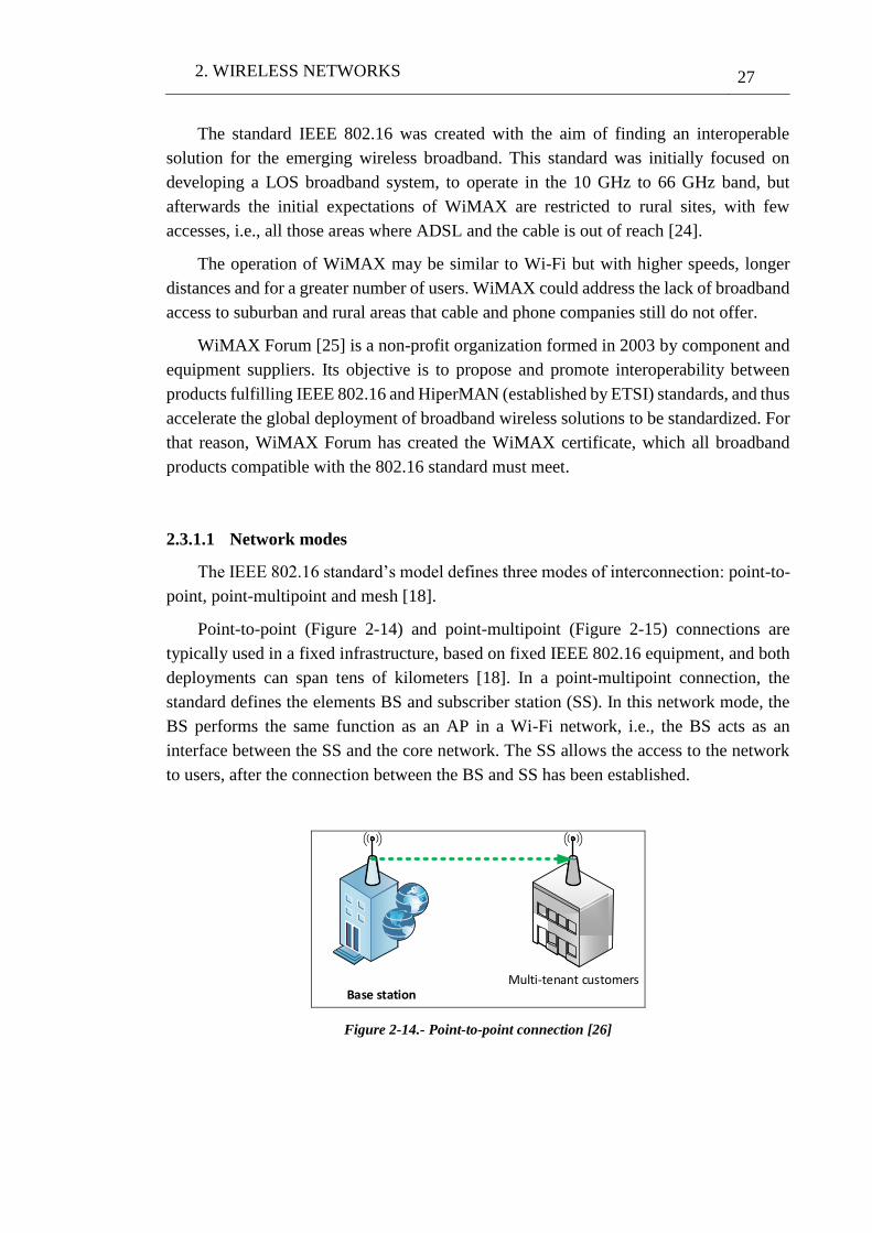
2. WIRELESS NETWORKS 27
The standard IEEE 802.16 was created with the aim of finding an interoperable
solution for the emerging wireless broadband. This standard was initially focused on
developing a LOS broadband system, to operate in the 10 GHz to 66 GHz band, but
afterwards the initial expectations of WiMAX are restricted to rural sites, with few
accesses, i.e., all those areas where ADSL and the cable is out of reach [24].
The operation of WiMAX may be similar to Wi-Fi but with higher speeds, longer
distances and for a greater number of users. WiMAX could address the lack of broadband
access to suburban and rural areas that cable and phone companies still do not offer.
WiMAX Forum [25] is a non-profit organization formed in 2003 by component and
equipment suppliers. Its objective is to propose and promote interoperability between
products fulfilling IEEE 802.16 and HiperMAN (established by ETSI) standards, and thus
accelerate the global deployment of broadband wireless solutions to be standardized. For
that reason, WiMAX Forum has created the WiMAX certificate, which all broadband
products compatible with the 802.16 standard must meet.
2.3.1.1 Network modes
The IEEE 802.16 standard’s model defines three modes of interconnection: point-to-
point, point-multipoint and mesh [18].
Point-to-point (Figure 2-14) and point-multipoint (Figure 2-15) connections are
typically used in a fixed infrastructure, based on fixed IEEE 802.16 equipment, and both
deployments can span tens of kilometers [18]. In a point-multipoint connection, the
standard defines the elements BS and subscriber station (SS). In this network mode, the
BS performs the same function as an AP in a Wi-Fi network, i.e., the BS acts as an
interface between the SS and the core network. The SS allows the access to the network
to users, after the connection between the BS and SS has been established.
Base stationMulti-tenant customers
Figure 2-14.- Point-to-point connection [26]
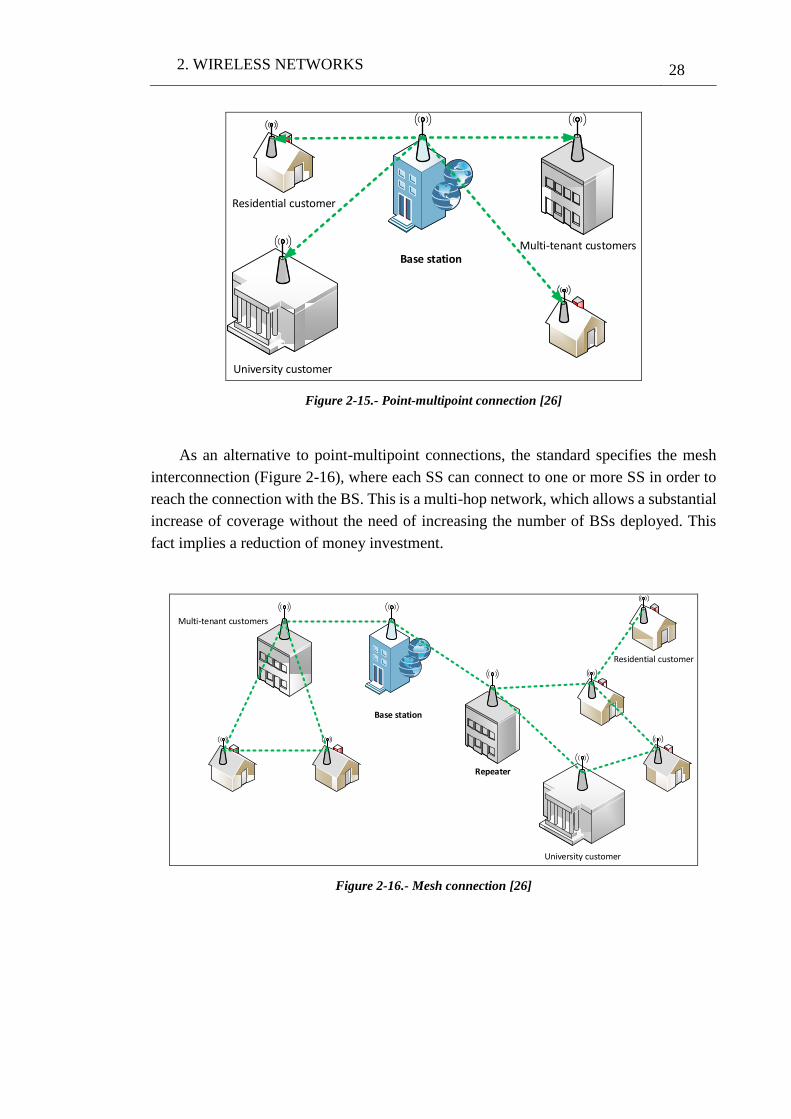
2. WIRELESS NETWORKS 28
Base stationMulti-tenant customers
Residential customer
University customer
Figure 2-15.- Point-multipoint connection [26]
As an alternative to point-multipoint connections, the standard specifies the mesh
interconnection (Figure 2-16), where each SS can connect to one or more SS in order to
reach the connection with the BS. This is a multi-hop network, which allows a substantial
increase of coverage without the need of increasing the number of BSs deployed. This
fact implies a reduction of money investment.
Base station
University customer
Repeater
Residential customer
Multi-tenant customers
Figure 2-16.- Mesh connection [26]
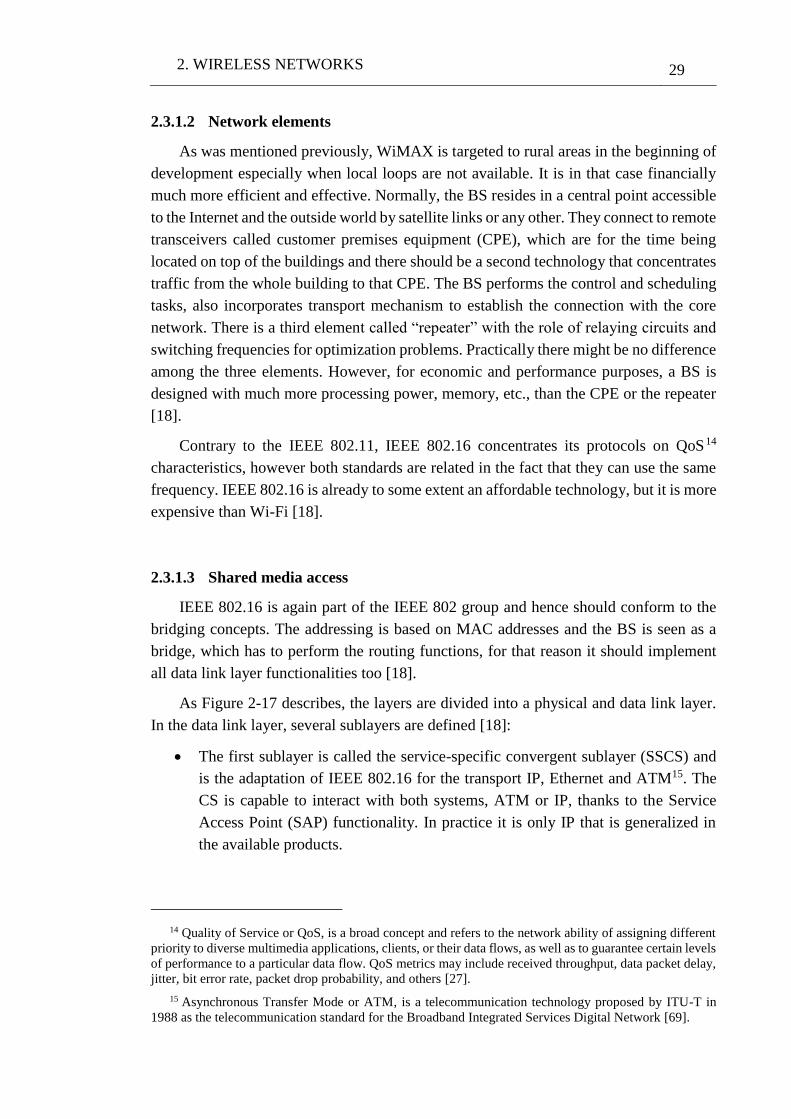
2. WIRELESS NETWORKS 29
2.3.1.2 Network elements
As was mentioned previously, WiMAX is targeted to rural areas in the beginning of
development especially when local loops are not available. It is in that case financially
much more efficient and effective. Normally, the BS resides in a central point accessible
to the Internet and the outside world by satellite links or any other. They connect to remote
transceivers called customer premises equipment (CPE), which are for the time being
located on top of the buildings and there should be a second technology that concentrates
traffic from the whole building to that CPE. The BS performs the control and scheduling
tasks, also incorporates transport mechanism to establish the connection with the core
network. There is a third element called “repeater” with the role of relaying circuits and
switching frequencies for optimization problems. Practically there might be no difference
among the three elements. However, for economic and performance purposes, a BS is
designed with much more processing power, memory, etc., than the CPE or the repeater
[18].
Contrary to the IEEE 802.11, IEEE 802.16 concentrates its protocols on QoS14
characteristics, however both standards are related in the fact that they can use the same
frequency. IEEE 802.16 is already to some extent an affordable technology, but it is more
expensive than Wi-Fi [18].
2.3.1.3 Shared media access
IEEE 802.16 is again part of the IEEE 802 group and hence should conform to the
bridging concepts. The addressing is based on MAC addresses and the BS is seen as a
bridge, which has to perform the routing functions, for that reason it should implement
all data link layer functionalities too [18].
As Figure 2-17 describes, the layers are divided into a physical and data link layer.
In the data link layer, several sublayers are defined [18]:
The first sublayer is called the service-specific convergent sublayer (SSCS) and
is the adaptation of IEEE 802.16 for the transport IP, Ethernet and ATM15. The
CS is capable to interact with both systems, ATM or IP, thanks to the Service
Access Point (SAP) functionality. In practice it is only IP that is generalized in
the available products.
14 Quality of Service or QoS, is a broad concept and refers to the network ability of assigning different
priority to diverse multimedia applications, clients, or their data flows, as well as to guarantee certain levels
of performance to a particular data flow. QoS metrics may include received throughput, data packet delay,
jitter, bit error rate, packet drop probability, and others [27].
15 Asynchronous Transfer Mode or ATM, is a telecommunication technology proposed by ITU-T in
1988 as the telecommunication standard for the Broadband Integrated Services Digital Network [69].
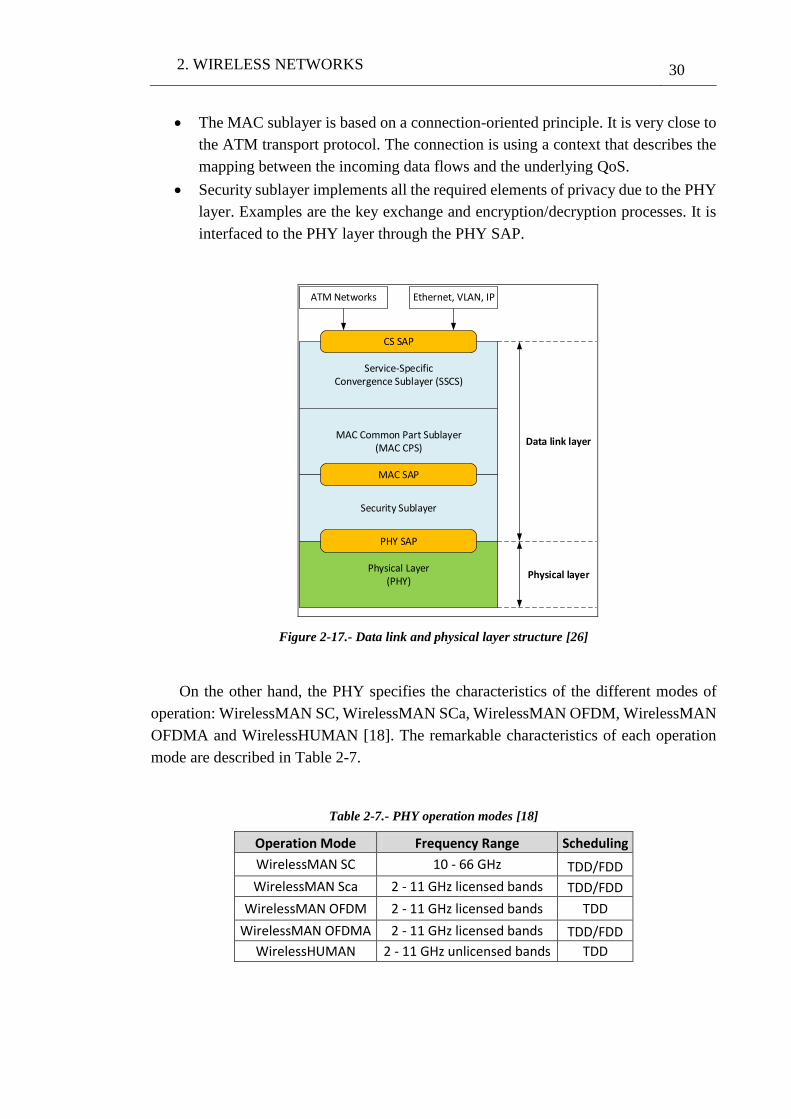
2. WIRELESS NETWORKS 30
The MAC sublayer is based on a connection-oriented principle. It is very close to
the ATM transport protocol. The connection is using a context that describes the
mapping between the incoming data flows and the underlying QoS.
Security sublayer implements all the required elements of privacy due to the PHY
layer. Examples are the key exchange and encryption/decryption processes. It is
interfaced to the PHY layer through the PHY SAP.
Service-SpecificConvergence Sublayer (SSCS)
MAC Common Part Sublayer(MAC CPS)
Security Sublayer
Physical Layer(PHY)
CS SAP
MAC SAP
PHY SAP
Physical layer
Data link layer
ATM Networks Ethernet, VLAN, IP
Figure 2-17.- Data link and physical layer structure [26]
On the other hand, the PHY specifies the characteristics of the different modes of
operation: WirelessMAN SC, WirelessMAN SCa, WirelessMAN OFDM, WirelessMAN
OFDMA and WirelessHUMAN [18]. The remarkable characteristics of each operation
mode are described in Table 2-7.
Table 2-7.- PHY operation modes [18]
Operation Mode Frequency Range Scheduling
WirelessMAN SC 10 - 66 GHz TDD/FDD
WirelessMAN Sca 2 - 11 GHz licensed bands TDD/FDD
WirelessMAN OFDM 2 - 11 GHz licensed bands TDD
WirelessMAN OFDMA 2 - 11 GHz licensed bands TDD/FDD
WirelessHUMAN 2 - 11 GHz unlicensed bands TDD
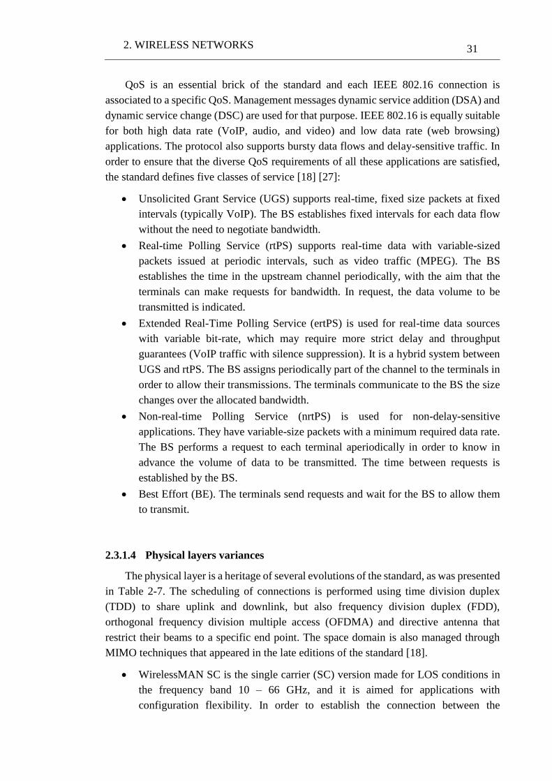
2. WIRELESS NETWORKS 31
QoS is an essential brick of the standard and each IEEE 802.16 connection is
associated to a specific QoS. Management messages dynamic service addition (DSA) and
dynamic service change (DSC) are used for that purpose. IEEE 802.16 is equally suitable
for both high data rate (VoIP, audio, and video) and low data rate (web browsing)
applications. The protocol also supports bursty data flows and delay-sensitive traffic. In
order to ensure that the diverse QoS requirements of all these applications are satisfied,
the standard defines five classes of service [18] [27]:
Unsolicited Grant Service (UGS) supports real-time, fixed size packets at fixed
intervals (typically VoIP). The BS establishes fixed intervals for each data flow
without the need to negotiate bandwidth.
Real-time Polling Service (rtPS) supports real-time data with variable-sized
packets issued at periodic intervals, such as video traffic (MPEG). The BS
establishes the time in the upstream channel periodically, with the aim that the
terminals can make requests for bandwidth. In request, the data volume to be
transmitted is indicated.
Extended Real-Time Polling Service (ertPS) is used for real-time data sources
with variable bit-rate, which may require more strict delay and throughput
guarantees (VoIP traffic with silence suppression). It is a hybrid system between
UGS and rtPS. The BS assigns periodically part of the channel to the terminals in
order to allow their transmissions. The terminals communicate to the BS the size
changes over the allocated bandwidth.
Non-real-time Polling Service (nrtPS) is used for non-delay-sensitive
applications. They have variable-size packets with a minimum required data rate.
The BS performs a request to each terminal aperiodically in order to know in
advance the volume of data to be transmitted. The time between requests is
established by the BS.
Best Effort (BE). The terminals send requests and wait for the BS to allow them
to transmit.
2.3.1.4 Physical layers variances
The physical layer is a heritage of several evolutions of the standard, as was presented
in Table 2-7. The scheduling of connections is performed using time division duplex
(TDD) to share uplink and downlink, but also frequency division duplex (FDD),
orthogonal frequency division multiple access (OFDMA) and directive antenna that
restrict their beams to a specific end point. The space domain is also managed through
MIMO techniques that appeared in the late editions of the standard [18].
WirelessMAN SC is the single carrier (SC) version made for LOS conditions in
the frequency band 10 – 66 GHz, and it is aimed for applications with
configuration flexibility. In order to establish the connection between the
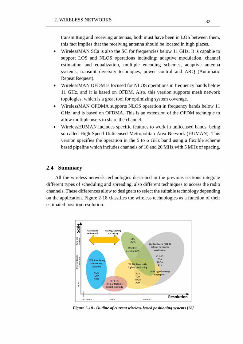
2. WIRELESS NETWORKS 32
transmitting and receiving antennas, both must have been in LOS between them,
this fact implies that the receiving antenna should be located in high places.
WirelessMAN SCa is also the SC for frequencies below 11 GHz. It is capable to
support LOS and NLOS operations including: adaptive modulation, channel
estimation and equalization, multiple encoding schemes, adaptive antenna
systems, transmit diversity techniques, power control and ARQ (Automatic
Repeat Request).
WirelessMAN OFDM is focused for NLOS operations in frequency bands below
11 GHz, and it is based on OFDM. Also, this version supports mesh network
topologies, which is a great tool for optimizing system coverage.
WirelessMAN OFDMA supports NLOS operation in frequency bands below 11
GHz, and is based on OFDMA. This is an extension of the OFDM technique to
allow multiple users to share the channel.
WirelessHUMAN includes specific features to work in unlicensed bands, being
so-called High Speed Unlicensed Metropolitan Area Network (HUMAN). This
version specifies the operation in the 5 to 6 GHz band using a flexible scheme
based pipeline which includes channels of 10 and 20 MHz with 5 MHz of spacing.
Summary
All the wireless network technologies described in the previous sections integrate
different types of scheduling and spreading, also different techniques to access the radio
channels. These differences allow to designers to select the suitable technology depending
on the application. Figure 2-18 classifies the wireless technologies as a function of their
estimated position resolution.
Resolution0.1 meters
Ind
oors
Scal
eO
utd
oor
Loca
lly
and
Urb
anR
ural
an
d R
emo
te
UWB, Propietary microwave solutions
AOATDOARTOF
RF & IR,RF & Ultrasonic hybrid methods
1 meter 10 meters
Automation and control
Guiding, tracking and routing
WLAN, Bluetooth, ZigBee positioning
RSSTOA
TDOAAOA
1G/2G/3G/4G mobile cellular networks
positioning
Cell-IDTOA
TDOARSS
Wide signal-strengt fingerprint
GPSDGPS
Wireless assisted GPS
Figure 2-18.- Outline of current wireless-based positioning systems [28]
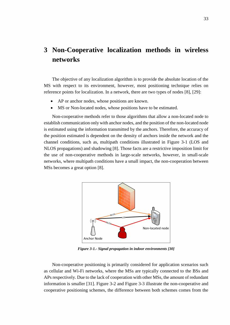
33
3 Non-Cooperative localization methods in wireless
networks
The objective of any localization algorithm is to provide the absolute location of the
MS with respect to its environment, however, most positioning technique relies on
reference points for localization. In a network, there are two types of nodes [8], [29]:
AP or anchor nodes, whose positions are known.
MS or Non-located nodes, whose positions have to be estimated.
Non-cooperative methods refer to those algorithms that allow a non-located node to
establish communication only with anchor nodes, and the position of the non-located node
is estimated using the information transmitted by the anchors. Therefore, the accuracy of
the position estimated is dependent on the density of anchors inside the network and the
channel conditions, such as, multipath conditions illustrated in Figure 3-1 (LOS and
NLOS propagations) and shadowing [8]. Those facts are a restrictive imposition limit for
the use of non-cooperative methods in large-scale networks, however, in small-scale
networks, where multipath conditions have a small impact, the non-cooperation between
MSs becomes a great option [8].
Anchor Node
Non-located node
Figure 3-1.- Signal propagation in indoor environments [30]
Non-cooperative positioning is primarily considered for application scenarios such
as cellular and Wi-Fi networks, where the MSs are typically connected to the BSs and
APs respectively. Due to the lack of cooperation with other MSs, the amount of redundant
information is smaller [31]. Figure 3-2 and Figure 3-3 illustrate the non-cooperative and
cooperative positioning schemes, the difference between both schemes comes from the
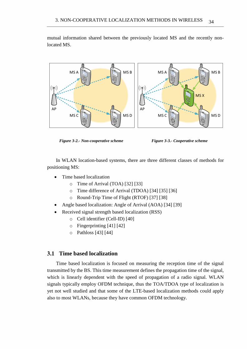
3. NON-COOPERATIVE LOCALIZATION METHODS IN WIRELESS 34
mutual information shared between the previously located MS and the recently non-
located MS.
AP
MS A MS B
MS C MS D
Figure 3-2.- Non-cooperative scheme
AP
MS X
MS A MS B
MS C MS D
Figure 3-3.- Cooperative scheme
In WLAN location-based systems, there are three different classes of methods for
positioning MS:
Time based localization
o Time of Arrival (TOA) [32] [33]
o Time difference of Arrival (TDOA) [34] [35] [36]
o Round-Trip Time of Flight (RTOF) [37] [38]
Angle based localization: Angle of Arrival (AOA) [34] [39]
Received signal strength based localization (RSS)
o Cell identifier (Cell-ID) [40]
o Fingerprinting [41] [42]
o Pathloss [43] [44]
Time based localization
Time based localization is focused on measuring the reception time of the signal
transmitted by the BS. This time measurement defines the propagation time of the signal,
which is linearly dependent with the speed of propagation of a radio signal. WLAN
signals typically employ OFDM technique, thus the TOA/TDOA type of localization is
yet not well studied and that some of the LTE-based localization methods could apply
also to most WLANs, because they have common OFDM technology.
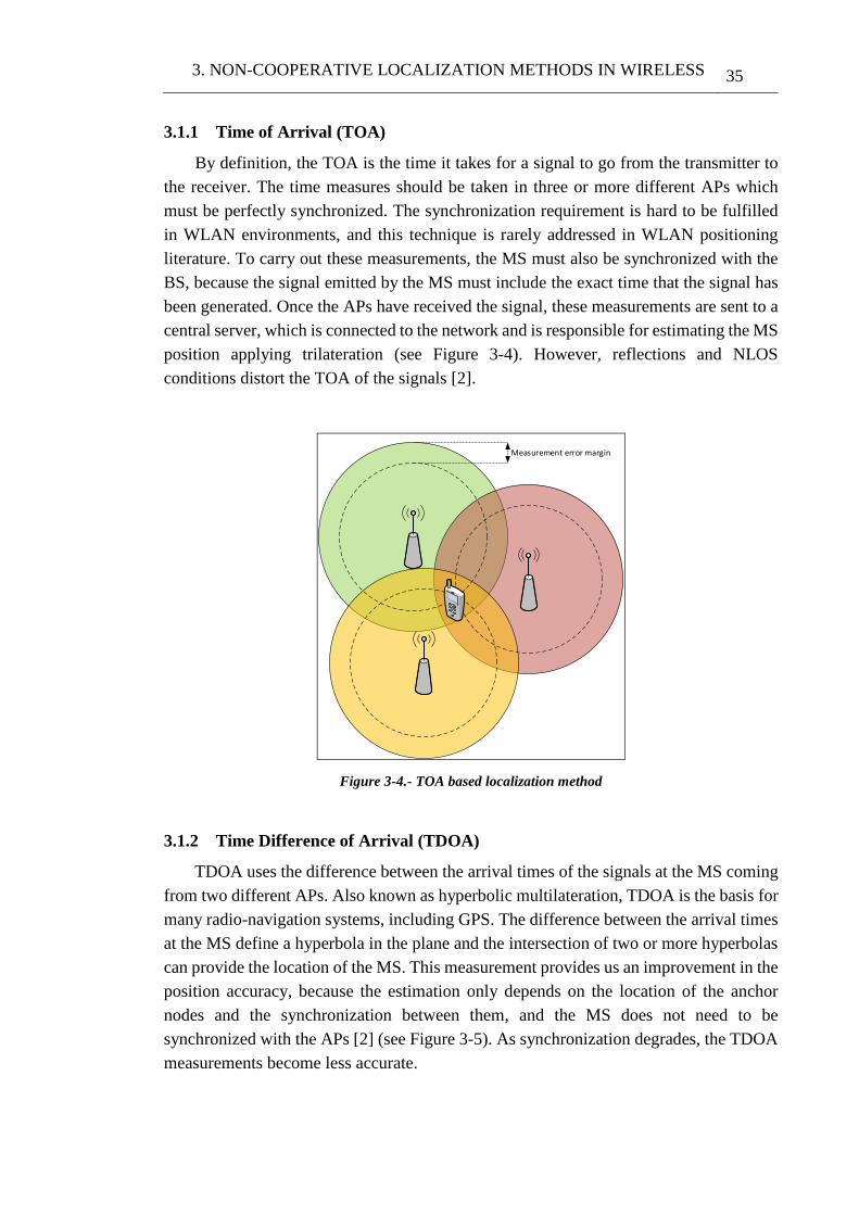
3. NON-COOPERATIVE LOCALIZATION METHODS IN WIRELESS 35
3.1.1 Time of Arrival (TOA)
By definition, the TOA is the time it takes for a signal to go from the transmitter to
the receiver. The time measures should be taken in three or more different APs which
must be perfectly synchronized. The synchronization requirement is hard to be fulfilled
in WLAN environments, and this technique is rarely addressed in WLAN positioning
literature. To carry out these measurements, the MS must also be synchronized with the
BS, because the signal emitted by the MS must include the exact time that the signal has
been generated. Once the APs have received the signal, these measurements are sent to a
central server, which is connected to the network and is responsible for estimating the MS
position applying trilateration (see Figure 3-4). However, reflections and NLOS
conditions distort the TOA of the signals [2].
Measurement error margin
Figure 3-4.- TOA based localization method
3.1.2 Time Difference of Arrival (TDOA)
TDOA uses the difference between the arrival times of the signals at the MS coming
from two different APs. Also known as hyperbolic multilateration, TDOA is the basis for
many radio-navigation systems, including GPS. The difference between the arrival times
at the MS define a hyperbola in the plane and the intersection of two or more hyperbolas
can provide the location of the MS. This measurement provides us an improvement in the
position accuracy, because the estimation only depends on the location of the anchor
nodes and the synchronization between them, and the MS does not need to be
synchronized with the APs [2] (see Figure 3-5). As synchronization degrades, the TDOA
measurements become less accurate.
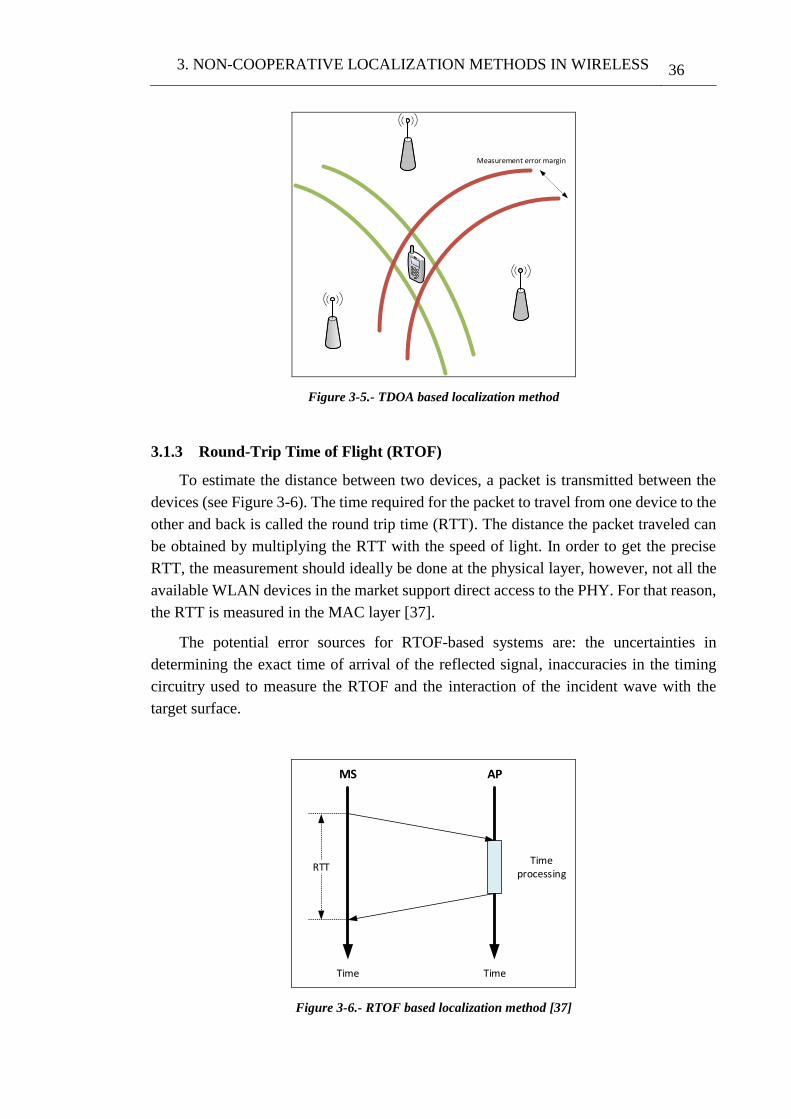
3. NON-COOPERATIVE LOCALIZATION METHODS IN WIRELESS 36
Measurement error margin
Figure 3-5.- TDOA based localization method
3.1.3 Round-Trip Time of Flight (RTOF)
To estimate the distance between two devices, a packet is transmitted between the
devices (see Figure 3-6). The time required for the packet to travel from one device to the
other and back is called the round trip time (RTT). The distance the packet traveled can
be obtained by multiplying the RTT with the speed of light. In order to get the precise
RTT, the measurement should ideally be done at the physical layer, however, not all the
available WLAN devices in the market support direct access to the PHY. For that reason,
the RTT is measured in the MAC layer [37].
The potential error sources for RTOF-based systems are: the uncertainties in
determining the exact time of arrival of the reflected signal, inaccuracies in the timing
circuitry used to measure the RTOF and the interaction of the incident wave with the
target surface.
Time
MS
Time
AP
Time processing
RTT
Figure 3-6.- RTOF based localization method [37]
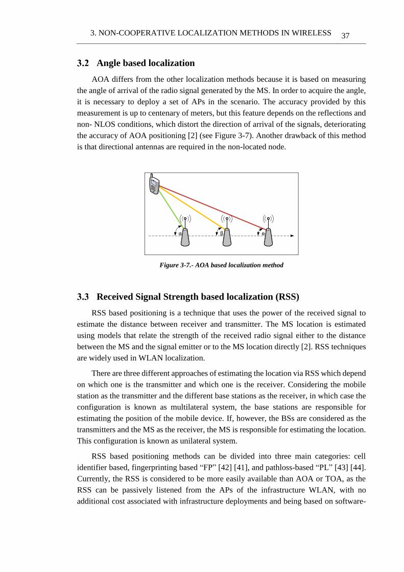
3. NON-COOPERATIVE LOCALIZATION METHODS IN WIRELESS 37
Angle based localization
AOA differs from the other localization methods because it is based on measuring
the angle of arrival of the radio signal generated by the MS. In order to acquire the angle,
it is necessary to deploy a set of APs in the scenario. The accuracy provided by this
measurement is up to centenary of meters, but this feature depends on the reflections and
non- NLOS conditions, which distort the direction of arrival of the signals, deteriorating
the accuracy of AOA positioning [2] (see Figure 3-7). Another drawback of this method
is that directional antennas are required in the non-located node.
α β ɵ
Figure 3-7.- AOA based localization method
Received Signal Strength based localization (RSS)
RSS based positioning is a technique that uses the power of the received signal to
estimate the distance between receiver and transmitter. The MS location is estimated
using models that relate the strength of the received radio signal either to the distance
between the MS and the signal emitter or to the MS location directly [2]. RSS techniques
are widely used in WLAN localization.
There are three different approaches of estimating the location via RSS which depend
on which one is the transmitter and which one is the receiver. Considering the mobile
station as the transmitter and the different base stations as the receiver, in which case the
configuration is known as multilateral system, the base stations are responsible for
estimating the position of the mobile device. If, however, the BSs are considered as the
transmitters and the MS as the receiver, the MS is responsible for estimating the location.
This configuration is known as unilateral system.
RSS based positioning methods can be divided into three main categories: cell
identifier based, fingerprinting based “FP” [42] [41], and pathloss-based “PL” [43] [44].
Currently, the RSS is considered to be more easily available than AOA or TOA, as the
RSS can be passively listened from the APs of the infrastructure WLAN, with no
additional cost associated with infrastructure deployments and being based on software-
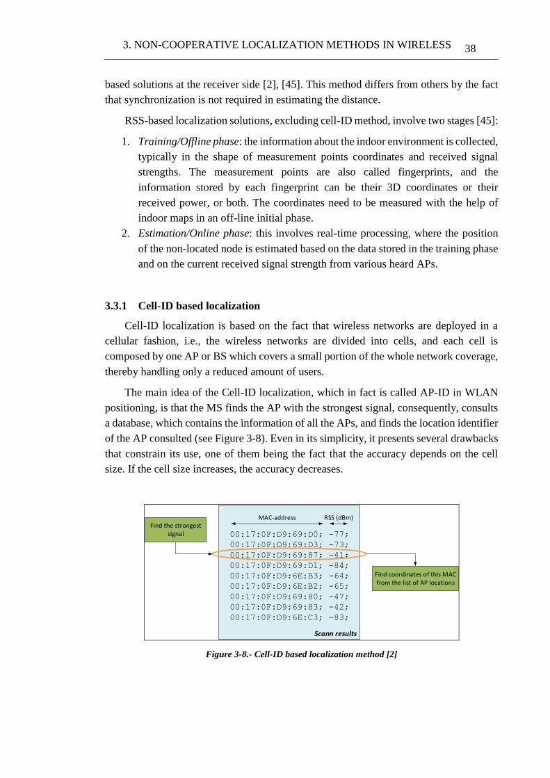
3. NON-COOPERATIVE LOCALIZATION METHODS IN WIRELESS 38
based solutions at the receiver side [2], [45]. This method differs from others by the fact
that synchronization is not required in estimating the distance.
RSS-based localization solutions, excluding cell-ID method, involve two stages [45]:
1. Training/Offline phase: the information about the indoor environment is collected,
typically in the shape of measurement points coordinates and received signal
strengths. The measurement points are also called fingerprints, and the
information stored by each fingerprint can be their 3D coordinates or their
received power, or both. The coordinates need to be measured with the help of
indoor maps in an off-line initial phase.
2. Estimation/Online phase: this involves real-time processing, where the position
of the non-located node is estimated based on the data stored in the training phase
and on the current received signal strength from various heard APs.
3.3.1 Cell-ID based localization
Cell-ID localization is based on the fact that wireless networks are deployed in a
cellular fashion, i.e., the wireless networks are divided into cells, and each cell is
composed by one AP or BS which covers a small portion of the whole network coverage,
thereby handling only a reduced amount of users.
The main idea of the Cell-ID localization, which in fact is called AP-ID in WLAN
positioning, is that the MS finds the AP with the strongest signal, consequently, consults
a database, which contains the information of all the APs, and finds the location identifier
of the AP consulted (see Figure 3-8). Even in its simplicity, it presents several drawbacks
that constrain its use, one of them being the fact that the accuracy depends on the cell
size. If the cell size increases, the accuracy decreases.
00:17:0F:D9:69:D0; -77;
00:17:0F:D9:69:D3; -73;
00:17:0F:D9:69:87; -41;
00:17:0F:D9:69:D1; -84;
00:17:0F:D9:6E:B3; -64;
00:17:0F:D9:6E:B2; -65;
00:17:0F:D9:69:80; -47;
00:17:0F:D9:69:83; -42;
00:17:0F:D9:6E:C3; -83;
RSS (dBm)MAC-address
Scann results
Find the strongest signal
Find coordinates of this MAC from the list of AP locations
Figure 3-8.- Cell-ID based localization method [2]
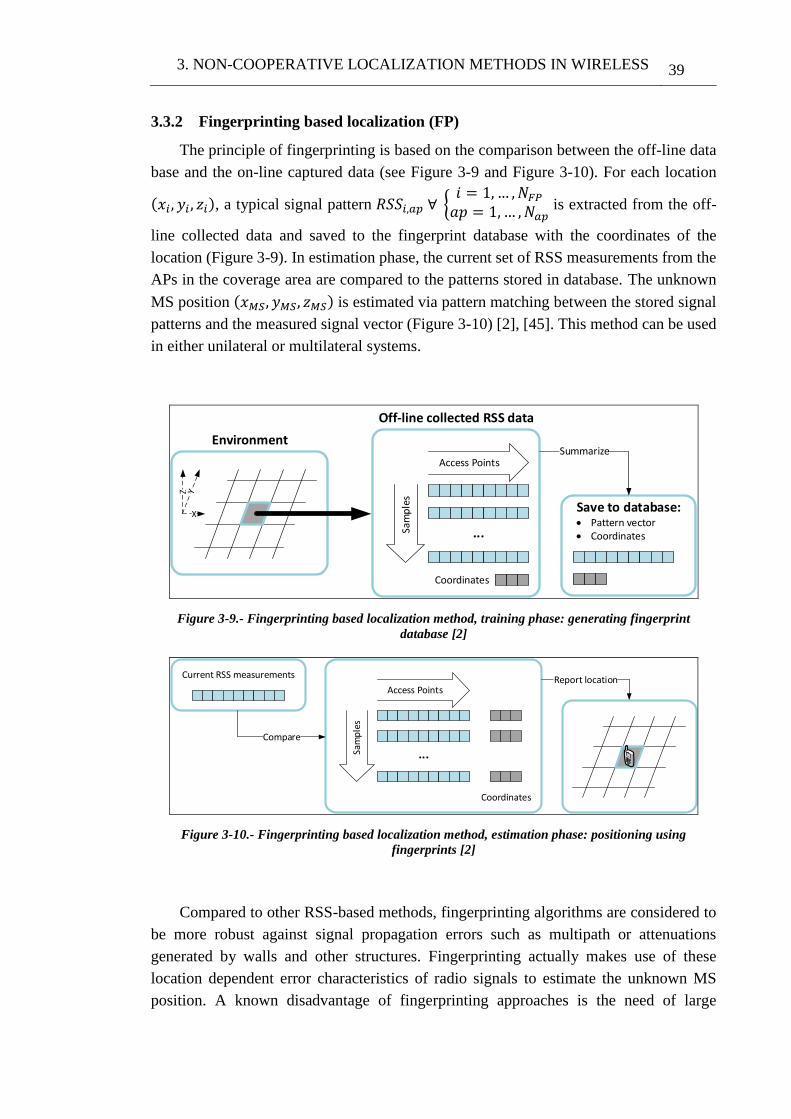
3. NON-COOPERATIVE LOCALIZATION METHODS IN WIRELESS 39
3.3.2 Fingerprinting based localization (FP)
The principle of fingerprinting is based on the comparison between the off-line data
base and the on-line captured data (see Figure 3-9 and Figure 3-10). For each location
(𝑥𝑖, 𝑦𝑖 , 𝑧𝑖), a typical signal pattern 𝑅𝑆𝑆𝑖,𝑎𝑝 ∀ {𝑖 = 1,… ,𝑁𝐹𝑃
𝑎𝑝 = 1,… ,𝑁𝑎𝑝 is extracted from the off-
line collected data and saved to the fingerprint database with the coordinates of the
location (Figure 3-9). In estimation phase, the current set of RSS measurements from the
APs in the coverage area are compared to the patterns stored in database. The unknown
MS position (𝑥𝑀𝑆, 𝑦𝑀𝑆, 𝑧𝑀𝑆) is estimated via pattern matching between the stored signal
patterns and the measured signal vector (Figure 3-10) [2], [45]. This method can be used
in either unilateral or multilateral systems.
···Sam
ple
s
Access Points
Coordinates
Off-line collected RSS data
Environment
Save to database: Pattern vector Coordinates
X
Z
Summarize
Figure 3-9.- Fingerprinting based localization method, training phase: generating fingerprint
database [2]
Current RSS measurements
···Sam
ple
s
Access Points
Coordinates
Compare
Report location
Figure 3-10.- Fingerprinting based localization method, estimation phase: positioning using
fingerprints [2]
Compared to other RSS-based methods, fingerprinting algorithms are considered to
be more robust against signal propagation errors such as multipath or attenuations
generated by walls and other structures. Fingerprinting actually makes use of these
location dependent error characteristics of radio signals to estimate the unknown MS
position. A known disadvantage of fingerprinting approaches is the need of large
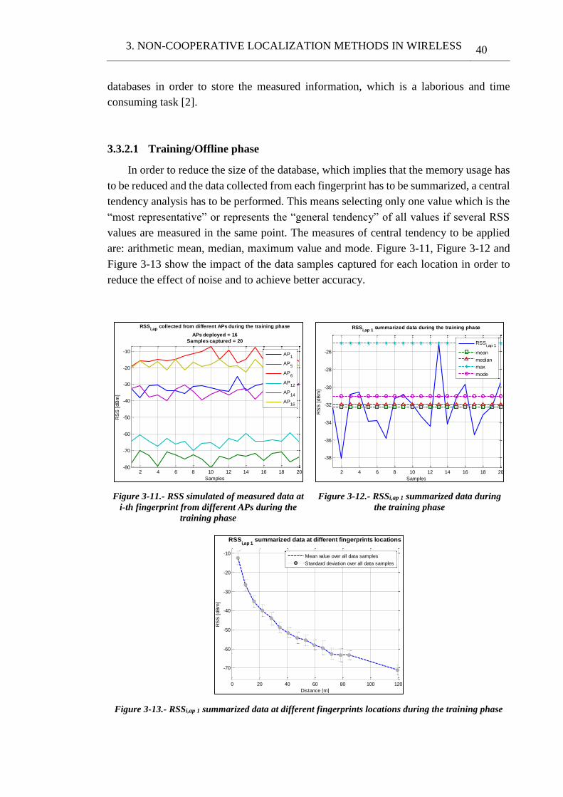
3. NON-COOPERATIVE LOCALIZATION METHODS IN WIRELESS 40
databases in order to store the measured information, which is a laborious and time
consuming task [2].
3.3.2.1 Training/Offline phase
In order to reduce the size of the database, which implies that the memory usage has
to be reduced and the data collected from each fingerprint has to be summarized, a central
tendency analysis has to be performed. This means selecting only one value which is the
“most representative” or represents the “general tendency” of all values if several RSS
values are measured in the same point. The measures of central tendency to be applied
are: arithmetic mean, median, maximum value and mode. Figure 3-11, Figure 3-12 and
Figure 3-13 show the impact of the data samples captured for each location in order to
reduce the effect of noise and to achieve better accuracy.
Figure 3-11.- RSS simulated of measured data at
i-th fingerprint from different APs during the
training phase
Figure 3-12.- RSSi,ap 1 summarized data during
the training phase
Figure 3-13.- RSSi,ap 1 summarized data at different fingerprints locations during the training phase
2 4 6 8 10 12 14 16 18 20-80
-70
-60
-50
-40
-30
-20
-10
Samples
RS
S [
dB
m]
RSSi,ap
collected from different APs during the training phase
APs deployed = 16
Samples captured = 20
AP1
AP5
AP6
AP12
AP14
AP16
2 4 6 8 10 12 14 16 18 20
-38
-36
-34
-32
-30
-28
-26
Samples
RS
S [
dB
m]
RSSi,ap 1
summarized data during the training phase
RSSi,ap 1
mean
median
max
mode
0 20 40 60 80 100 120
-70
-60
-50
-40
-30
-20
-10
Distance [m]
RS
S [
dB
m]
RSSi,ap 1
summarized data at different fingerprints locations
Mean value over all data samples
Standard deviation over all data samples
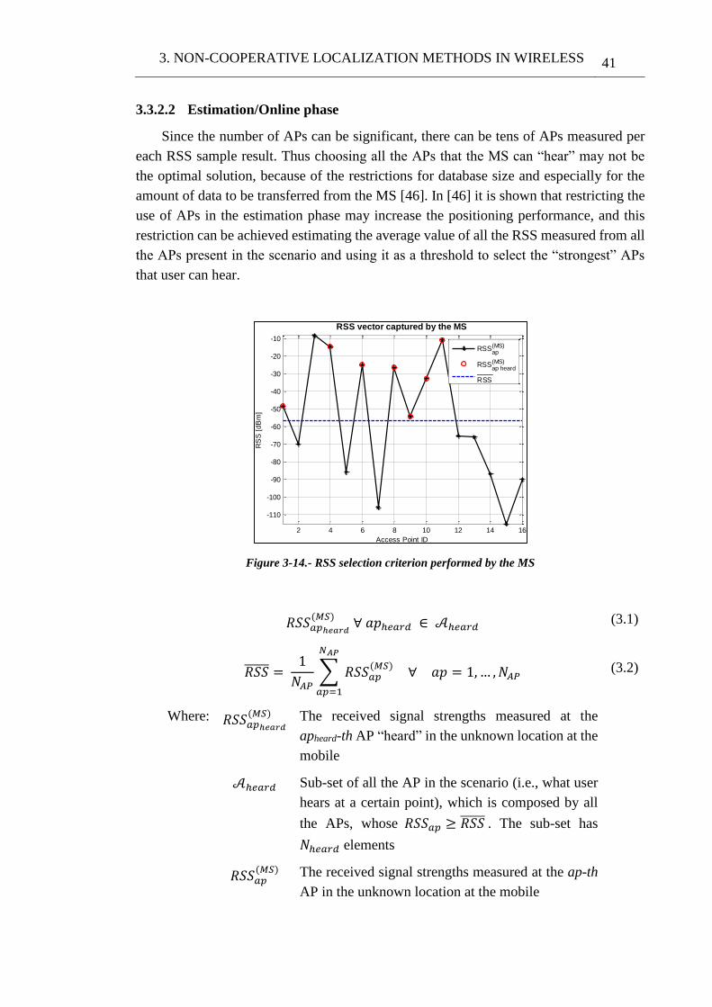
3. NON-COOPERATIVE LOCALIZATION METHODS IN WIRELESS 41
3.3.2.2 Estimation/Online phase
Since the number of APs can be significant, there can be tens of APs measured per
each RSS sample result. Thus choosing all the APs that the MS can “hear” may not be
the optimal solution, because of the restrictions for database size and especially for the
amount of data to be transferred from the MS [46]. In [46] it is shown that restricting the
use of APs in the estimation phase may increase the positioning performance, and this
restriction can be achieved estimating the average value of all the RSS measured from all
the APs present in the scenario and using it as a threshold to select the “strongest” APs
that user can hear.
Figure 3-14.- RSS selection criterion performed by the MS
𝑅𝑆𝑆𝑎𝑝ℎ𝑒𝑎𝑟𝑑
(𝑀𝑆) ∀ 𝑎𝑝ℎ𝑒𝑎𝑟𝑑 ∈ 𝒜ℎ𝑒𝑎𝑟𝑑 (3.1)
𝑅𝑆𝑆̅̅ ̅̅ ̅ = 1
𝑁𝐴𝑃∑ 𝑅𝑆𝑆𝑎𝑝
(𝑀𝑆)
𝑁𝐴𝑃
𝑎𝑝=1
∀ 𝑎𝑝 = 1,… ,𝑁𝐴𝑃 (3.2)
Where: 𝑅𝑆𝑆𝑎𝑝ℎ𝑒𝑎𝑟𝑑
(𝑀𝑆) The received signal strengths measured at the
apheard-th AP “heard” in the unknown location at the
mobile
𝒜ℎ𝑒𝑎𝑟𝑑 Sub-set of all the AP in the scenario (i.e., what user
hears at a certain point), which is composed by all
the APs, whose 𝑅𝑆𝑆𝑎𝑝 ≥ 𝑅𝑆𝑆̅̅ ̅̅ ̅ . The sub-set has
𝑁ℎ𝑒𝑎𝑟𝑑 elements
𝑅𝑆𝑆𝑎𝑝(𝑀𝑆)
The received signal strengths measured at the ap-th
AP in the unknown location at the mobile
2 4 6 8 10 12 14 16
-110
-100
-90
-80
-70
-60
-50
-40
-30
-20
-10
Access Point ID
RS
S [
dB
m]
RSS vector captured by the MS
RSSap(MS)
RSSap heard(MS)
RSS
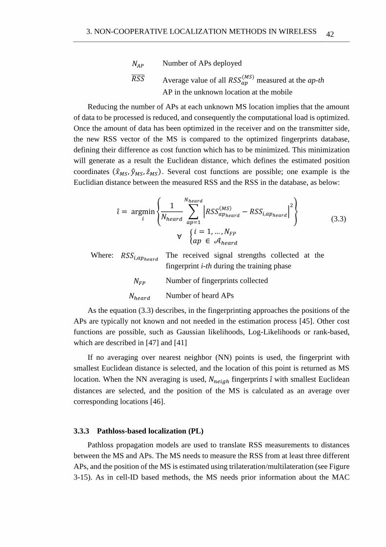
3. NON-COOPERATIVE LOCALIZATION METHODS IN WIRELESS 42
𝑁𝐴𝑃 Number of APs deployed
𝑅𝑆𝑆̅̅ ̅̅ ̅ Average value of all 𝑅𝑆𝑆𝑎𝑝(𝑀𝑆)
measured at the ap-th
AP in the unknown location at the mobile
Reducing the number of APs at each unknown MS location implies that the amount
of data to be processed is reduced, and consequently the computational load is optimized.
Once the amount of data has been optimized in the receiver and on the transmitter side,
the new RSS vector of the MS is compared to the optimized fingerprints database,
defining their difference as cost function which has to be minimized. This minimization
will generate as a result the Euclidean distance, which defines the estimated position
coordinates (�̂�𝑀𝑆, �̂�𝑀𝑆, �̂�𝑀𝑆) . Several cost functions are possible; one example is the
Euclidian distance between the measured RSS and the RSS in the database, as below:
𝑖̂ = argmin𝑖
{1
𝑁ℎ𝑒𝑎𝑟𝑑∑ |𝑅𝑆𝑆𝑎𝑝ℎ𝑒𝑎𝑟𝑑
(𝑀𝑆)− 𝑅𝑆𝑆𝑖,𝑎𝑝ℎ𝑒𝑎𝑟𝑑
|2
𝑁ℎ𝑒𝑎𝑟𝑑
𝑎𝑝=1
}
∀ {𝑖 = 1,… ,𝑁𝐹𝑃
𝑎𝑝 ∈ 𝒜ℎ𝑒𝑎𝑟𝑑
(3.3)
Where: 𝑅𝑆𝑆𝑖,𝑎𝑝ℎ𝑒𝑎𝑟𝑑 The received signal strengths collected at the
fingerprint i-th during the training phase
𝑁𝐹𝑃 Number of fingerprints collected
𝑁ℎ𝑒𝑎𝑟𝑑 Number of heard APs
As the equation (3.3) describes, in the fingerprinting approaches the positions of the
APs are typically not known and not needed in the estimation process [45]. Other cost
functions are possible, such as Gaussian likelihoods, Log-Likelihoods or rank-based,
which are described in [47] and [41]
If no averaging over nearest neighbor (NN) points is used, the fingerprint with
smallest Euclidean distance is selected, and the location of this point is returned as MS
location. When the NN averaging is used, 𝑁𝑛𝑒𝑖𝑔ℎ fingerprints 𝑖̂ with smallest Euclidean
distances are selected, and the position of the MS is calculated as an average over
corresponding locations [46].
3.3.3 Pathloss-based localization (PL)
Pathloss propagation models are used to translate RSS measurements to distances
between the MS and APs. The MS needs to measure the RSS from at least three different
APs, and the position of the MS is estimated using trilateration/multilateration (see Figure
3-15). As in cell-ID based methods, the MS needs prior information about the MAC
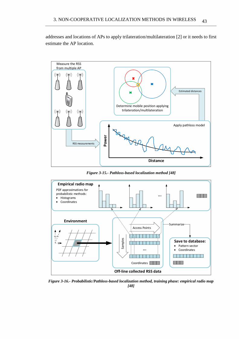
3. NON-COOPERATIVE LOCALIZATION METHODS IN WIRELESS 43
addresses and locations of APs to apply trilateration/multilateration [2] or it needs to first
estimate the AP location.
RSS measurements
Estimated distances
Po
we
r
Distance
Measure the RSS from multiple AP
Determine mobile position applying trilateration/multilateration
Apply pathloss model
Figure 3-15.- Pathloss-based localization method [48]
···Sam
ple
s
Access Points
Coordinates
Off-line collected RSS data
Environment
Save to database: Pattern vector Coordinates
X
Z
Summarize
Empirical radio map
···
PDF approximations for probabilistic methods: Histograms Coordinates
Figure 3-16.- Probabilistic/Pathloss-based localization method, training phase: empirical radio map
[48]
3. NON-COOPERATIVE LOCALIZATION METHODS IN WIRELESS 44
Additionally, instead of trilateration methods, it also is possible to use cost functions
similarly with FP case. In this case the measured RSS value is compared to a recreated
RSS value based on the path-loss model and on a grid created at the receiver side.
In indoor environments, multipath and attenuation caused by walls, other structures,
and even people complicate the modeling of signal propagation. Because of this, the
positioning errors in pathloss-based positioning are typically larger than in fingerprinting
[2].
In order to reduce the impact of the environmental effects, [43] and [45] describe a
method for dynamic estimation of the model parameters for each AP using learning data
collected at known positions. This method is known as Probabilistic/Pathloss method,
which describes an empirical radio map with an associated PDF 16 to describe the
propagation of the radio signals in the environment (see Figure 3-16). The number of
required pathloss parameters is kept small in order to keep down the computational
complexity and the amount of information required in the estimation phase [43]. Instead
of the original fingerprints, this method stores a few parameters per AP [45].
Alternatively, the path loss parameters can be estimated via deconvolution approaches,
such as LS and MMSE, as shown in [45].
3.3.3.1 Training/Offline phase
In the training phase, the pathloss model parameters for each AP are estimated within
the given database (𝑥𝑖, 𝑦𝑖, 𝑧𝑖) and 𝑃𝑅𝑋𝑖,𝑎𝑝. A pathloss model is a model for signal
attenuation in space and involves two modeling parameters per AP [43]. Let’s assume
that each AP can be characterized by a vector 𝛩𝐴𝑃 with 𝑀 parameters [45], according to
the following model:
{𝑃𝑅𝑋𝑖,𝑎𝑝
= 𝑓(𝑑𝑖,𝑎𝑝, 𝛩𝐴𝑃 )
𝛩𝐴𝑃 = [𝑃𝑇𝑋𝑎𝑝𝑛𝑎𝑝]
(3.4)
{
𝑃𝑅𝑋𝑖,𝑎𝑝= 𝑅𝑆𝑆𝑖,𝑎𝑝 = 𝑃𝑇𝑋𝑎𝑝
− 10𝑛𝑎𝑝 log10 𝑑𝑖,𝑎𝑝 + 𝜂𝑖,𝑎𝑝
𝑑𝑖,𝑎𝑝 = √(𝑥𝑖 − 𝑥𝑎𝑝)2+ (𝑦𝑖 − 𝑦𝑎𝑝)
2+ (𝑧𝑖 − 𝑧𝑎𝑝)
2 (3.5)
Where: 𝑃𝑅𝑋𝑖,𝑎𝑝 The received signal strengths collected and summarized
from the ap-th AP at the fingerprint i-th during the
training phase
𝑑𝑖,𝑎𝑝 The distance between the ap-th AP and the i-th
measurement point
16 Probability Density Function or PDF
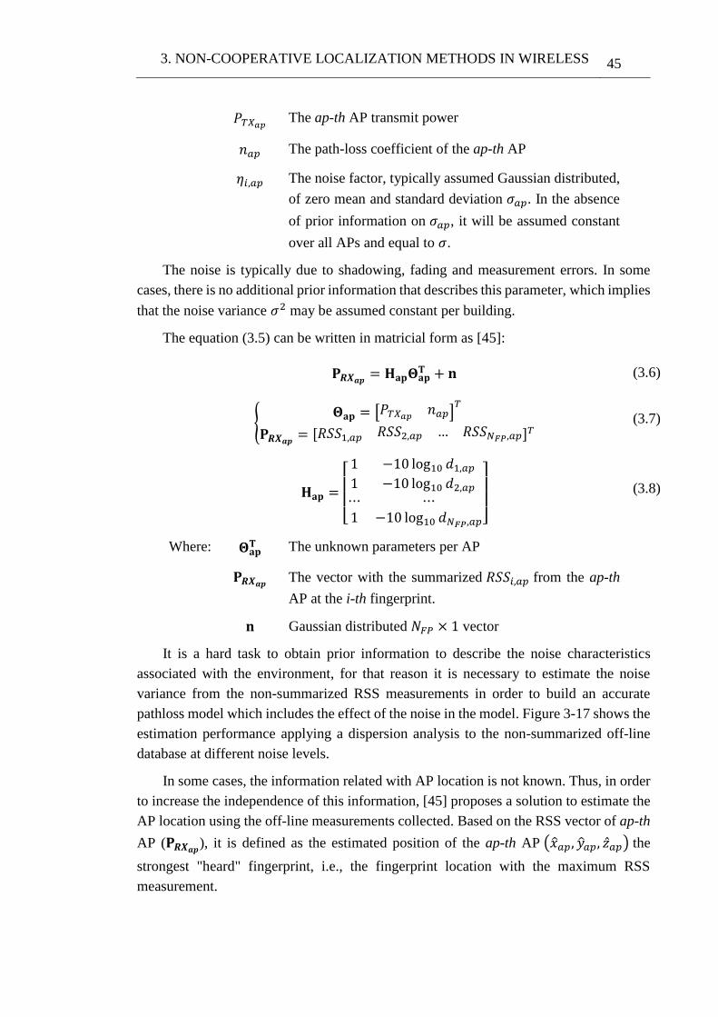
3. NON-COOPERATIVE LOCALIZATION METHODS IN WIRELESS 45
𝑃𝑇𝑋𝑎𝑝 The ap-th AP transmit power
𝑛𝑎𝑝 The path-loss coefficient of the ap-th AP
𝜂𝑖,𝑎𝑝 The noise factor, typically assumed Gaussian distributed,
of zero mean and standard deviation 𝜎𝑎𝑝. In the absence
of prior information on 𝜎𝑎𝑝, it will be assumed constant
over all APs and equal to 𝜎.
The noise is typically due to shadowing, fading and measurement errors. In some
cases, there is no additional prior information that describes this parameter, which implies
that the noise variance 𝜎2 may be assumed constant per building.
The equation (3.5) can be written in matricial form as [45]:
𝐏𝑹𝑿𝒂𝒑= 𝐇𝐚𝐩𝚯𝐚𝐩
𝐓 + 𝐧 (3.6)
{𝚯𝐚𝐩 = [𝑃𝑇𝑋𝑎𝑝
𝑛𝑎𝑝]𝑇
𝐏𝑹𝑿𝒂𝒑= [𝑅𝑆𝑆1,𝑎𝑝 𝑅𝑆𝑆2,𝑎𝑝 … 𝑅𝑆𝑆𝑁𝐹𝑃,𝑎𝑝]𝑇
(3.7)
𝐇𝐚𝐩 =
[ 1 −10 log10 𝑑1,𝑎𝑝
1 −10 log10 𝑑2,𝑎𝑝
⋯ ⋯1 −10 log10 𝑑𝑁𝐹𝑃,𝑎𝑝]
(3.8)
Where: 𝚯𝐚𝐩𝐓 The unknown parameters per AP
𝐏𝑹𝑿𝒂𝒑 The vector with the summarized 𝑅𝑆𝑆𝑖,𝑎𝑝 from the ap-th
AP at the i-th fingerprint.
𝐧 Gaussian distributed 𝑁𝐹𝑃 × 1 vector
It is a hard task to obtain prior information to describe the noise characteristics
associated with the environment, for that reason it is necessary to estimate the noise
variance from the non-summarized RSS measurements in order to build an accurate
pathloss model which includes the effect of the noise in the model. Figure 3-17 shows the
estimation performance applying a dispersion analysis to the non-summarized off-line
database at different noise levels.
In some cases, the information related with AP location is not known. Thus, in order
to increase the independence of this information, [45] proposes a solution to estimate the
AP location using the off-line measurements collected. Based on the RSS vector of ap-th
AP (𝐏𝑹𝑿𝒂𝒑), it is defined as the estimated position of the ap-th AP (�̂�𝑎𝑝, �̂�𝑎𝑝, �̂�𝑎𝑝) the
strongest "heard" fingerprint, i.e., the fingerprint location with the maximum RSS
measurement.
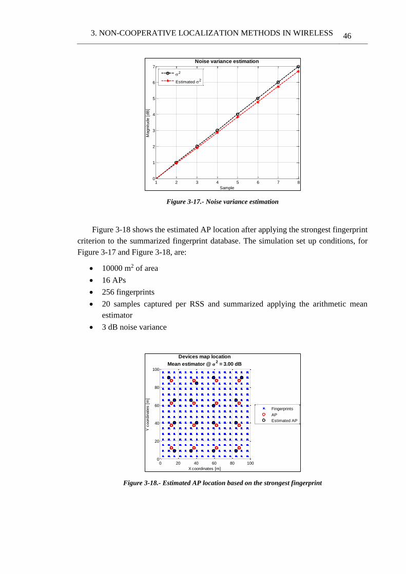
3. NON-COOPERATIVE LOCALIZATION METHODS IN WIRELESS 46
Figure 3-17.- Noise variance estimation
Figure 3-18 shows the estimated AP location after applying the strongest fingerprint
criterion to the summarized fingerprint database. The simulation set up conditions, for
Figure 3-17 and Figure 3-18, are:
10000 m2 of area
16 APs
256 fingerprints
20 samples captured per RSS and summarized applying the arithmetic mean
estimator
3 dB noise variance
Figure 3-18.- Estimated AP location based on the strongest fingerprint
1 2 3 4 5 6 7 80
1
2
3
4
5
6
7
Sample
Magnitude [
dB
]
Noise variance estimation
2
Estimated 2
0 20 40 60 80 1000
20
40
60
80
100
Devices map location
Mean estimator @ 2 = 3.00 dB
X coordinates [m]
Y c
oord
inate
s [
m]
Fingerprints
AP
Estimated AP
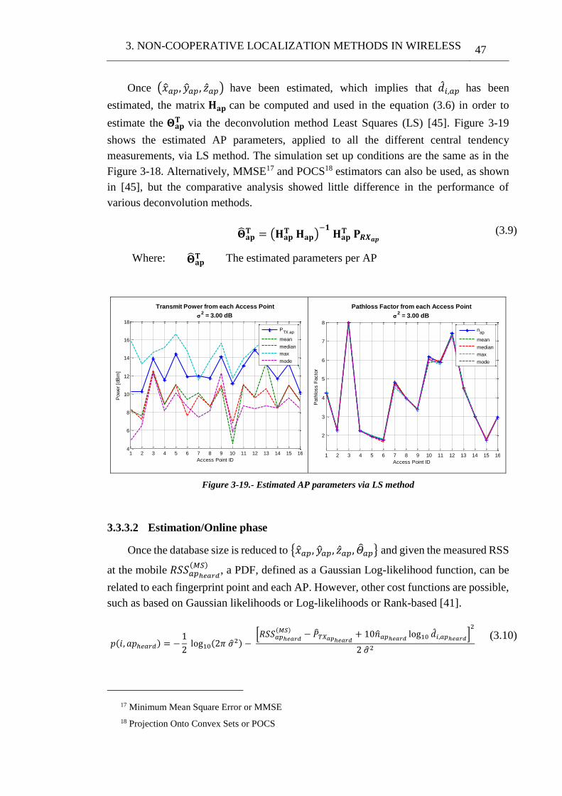
3. NON-COOPERATIVE LOCALIZATION METHODS IN WIRELESS 47
Once (�̂�𝑎𝑝, �̂�𝑎𝑝, �̂�𝑎𝑝) have been estimated, which implies that �̂�𝑖,𝑎𝑝 has been
estimated, the matrix 𝐇𝐚𝐩 can be computed and used in the equation (3.6) in order to
estimate the 𝚯𝐚𝐩𝐓 via the deconvolution method Least Squares (LS) [45]. Figure 3-19
shows the estimated AP parameters, applied to all the different central tendency
measurements, via LS method. The simulation set up conditions are the same as in the
Figure 3-18. Alternatively, MMSE17 and POCS18 estimators can also be used, as shown
in [45], but the comparative analysis showed little difference in the performance of
various deconvolution methods.
�̂�𝐚𝐩𝐓 = (𝐇𝐚𝐩
𝐓 𝐇𝐚𝐩)−𝟏
𝐇𝐚𝐩𝐓 𝐏𝑹𝑿𝒂𝒑
(3.9)
Where: �̂�𝐚𝐩𝐓 The estimated parameters per AP
Figure 3-19.- Estimated AP parameters via LS method
3.3.3.2 Estimation/Online phase
Once the database size is reduced to {�̂�𝑎𝑝, �̂�𝑎𝑝, �̂�𝑎𝑝, �̂�𝑎𝑝} and given the measured RSS
at the mobile 𝑅𝑆𝑆𝑎𝑝ℎ𝑒𝑎𝑟𝑑
(𝑀𝑆), a PDF, defined as a Gaussian Log-likelihood function, can be
related to each fingerprint point and each AP. However, other cost functions are possible,
such as based on Gaussian likelihoods or Log-likelihoods or Rank-based [41].
𝑝(𝑖, 𝑎𝑝ℎ𝑒𝑎𝑟𝑑) = −1
2 log10(2𝜋 �̂�2) −
[𝑅𝑆𝑆𝑎𝑝ℎ𝑒𝑎𝑟𝑑
(𝑀𝑆)− �̂�𝑇𝑋𝑎𝑝ℎ𝑒𝑎𝑟𝑑
+ 10�̂�𝑎𝑝ℎ𝑒𝑎𝑟𝑑log10 �̂�𝑖,𝑎𝑝ℎ𝑒𝑎𝑟𝑑
]2
2 �̂�2
(3.10)
17 Minimum Mean Square Error or MMSE
18 Projection Onto Convex Sets or POCS
1 2 3 4 5 6 7 8 9 10 11 12 13 14 15 164
6
8
10
12
14
16
18
Access Point ID
Pow
er
[dB
m]
Transmit Power from each Access Point
2 = 3.00 dB
PTX ap
mean
median
max
mode
1 2 3 4 5 6 7 8 9 10 11 12 13 14 15 16
2
3
4
5
6
7
8
Access Point ID
Path
loss F
acto
r
Pathloss Factor from each Access Point
2 = 3.00 dB
nap
mean
median
max
mode
3. NON-COOPERATIVE LOCALIZATION METHODS IN WIRELESS 48
Where: �̂�2 The estimated noise variance related to the 𝑅𝑆𝑆𝑖,𝑎𝑝
measurements
The problem of estimating the unknown MS location (�̂�𝑀𝑆, �̂�𝑀𝑆, �̂�𝑀𝑆) is reduced by
estimating the fingerprint 𝑖̂ which maximizes the PDF described in the equation (3.10).
𝑖̂ = argmax𝑖
{1
𝑁ℎ𝑒𝑎𝑟𝑑∑ |𝑝(𝑖, 𝑎𝑝ℎ𝑒𝑎𝑟𝑑)|2
𝑁ℎ𝑒𝑎𝑟𝑑
𝑎𝑝=1
}
∀ {𝑖 = 1,… ,𝑁𝐹𝑃
𝑎𝑝 ∈ 𝒜ℎ𝑒𝑎𝑟𝑑
(3.11)
Where: 𝑝(𝑖, 𝑎𝑝ℎ𝑒𝑎𝑟𝑑) The Gaussian Log-Likelihood function related to
each fingerprint point and for each AP
𝑁𝐹𝑃 Number on fingerprints collected
𝑁ℎ𝑒𝑎𝑟𝑑 The result of the equations (3.1) and (3.2) which
establish the number of heard APs
As was described in section 3.3.2.2, also averaging over 𝑁𝑛𝑒𝑖𝑔ℎ points can be used
in here and the position of the MS is calculated as an average over corresponding
locations.
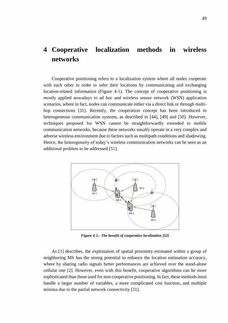
49
4 Cooperative localization methods in wireless
networks
Cooperative positioning refers to a localization system where all nodes cooperate
with each other in order to infer their locations by communicating and exchanging
location-related information (Figure 4-1). The concept of cooperative positioning is
mostly applied nowadays to ad hoc and wireless sensor network (WSN) application
scenarios, where in fact, nodes can communicate either via a direct link or through multi-
hop connections [31]. Recently, the cooperation concept has been introduced to
heterogeneous communication systems, as described in [44], [49] and [50]. However,
techniques proposed for WSN cannot be straightforwardly extended to mobile
communication networks, because these networks usually operate in a very complex and
adverse wireless environment due to factors such as multipath conditions and shadowing.
Hence, the heterogeneity of today’s wireless communication networks can be seen as an
additional problem to be addressed [51].
AP 1
AP 3
?
?AP 2
MS 2
MS 1
Figure 4-1.- The benefit of cooperative localization [52]
As [1] describes, the exploitation of spatial proximity estimated within a group of
neighboring MS has the strong potential to enhance the location estimation accuracy,
where by sharing radio signals better performances are achieved over the stand-alone
cellular one [2]. However, even with this benefit, cooperative algorithms can be more
sophisticated than those used for non-cooperative positioning. In fact, these methods must
handle a larger number of variables, a more complicated cost function, and multiple
minima due to the partial network connectivity [31].
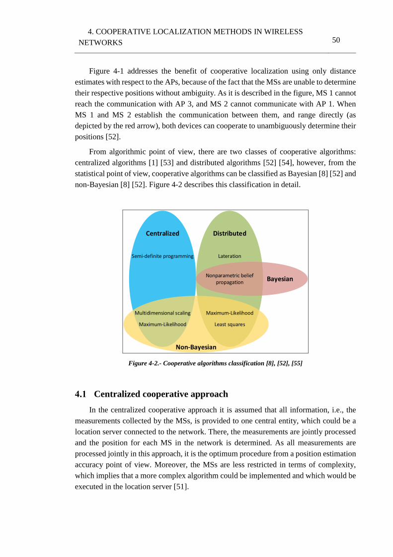
4. COOPERATIVE LOCALIZATION METHODS IN WIRELESS
NETWORKS 50
Figure 4-1 addresses the benefit of cooperative localization using only distance
estimates with respect to the APs, because of the fact that the MSs are unable to determine
their respective positions without ambiguity. As it is described in the figure, MS 1 cannot
reach the communication with AP 3, and MS 2 cannot communicate with AP 1. When
MS 1 and MS 2 establish the communication between them, and range directly (as
depicted by the red arrow), both devices can cooperate to unambiguously determine their
positions [52].
From algorithmic point of view, there are two classes of cooperative algorithms:
centralized algorithms [1] [53] and distributed algorithms [52] [54], however, from the
statistical point of view, cooperative algorithms can be classified as Bayesian [8] [52] and
non-Bayesian [8] [52]. Figure 4-2 describes this classification in detail.
Centralized Distributed
Non-Bayesian
Bayesian
Multidimensional scaling
Semi-definite programming
Maximum-Likelihood
Maximum-Likelihood
Least squares
Nonparametric belief propagation
Lateration
Figure 4-2.- Cooperative algorithms classification [8], [52], [55]
Centralized cooperative approach
In the centralized cooperative approach it is assumed that all information, i.e., the
measurements collected by the MSs, is provided to one central entity, which could be a
location server connected to the network. There, the measurements are jointly processed
and the position for each MS in the network is determined. As all measurements are
processed jointly in this approach, it is the optimum procedure from a position estimation
accuracy point of view. Moreover, the MSs are less restricted in terms of complexity,
which implies that a more complex algorithm could be implemented and which would be
executed in the location server [51].
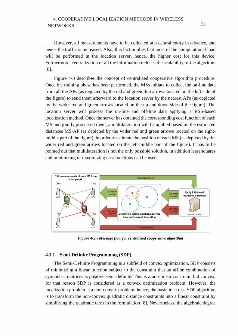
4. COOPERATIVE LOCALIZATION METHODS IN WIRELESS
NETWORKS 51
However, all measurements have to be collected at a central entity in advance, and
hence the traffic is increased. Also, this fact implies that most of the computational load
will be performed in the location server, hence, the higher cost for this device.
Furthermore, centralization of all the information reduces the scalability of the algorithm
[8].
Figure 4-3 describes the concept of centralized cooperative algorithm procedure.
Once the training phase has been performed, the MSs initiate to collect the on-line data
from all the APs (as depicted by the red and green thin arrows located on the left side of
the figure) to send them afterward to the location server by the nearest APs (as depicted
by the wider red and green arrows located on the up and down side of the figure). The
location server will process the on-line and off-line data applying a RSS-based
localization method. Once the server has obtained the corresponding cost function of each
MS and jointly processed them, a multilateration will be applied based on the estimated
distances MS-AP (as depicted by the wider red and green arrows located on the right-
middle part of the figure), in order to estimate the position of each MS (as depicted by the
wider red and green arrows located on the left-middle part of the figure). It has to be
pointed out that multilateration is not the only possible solution, in addition least squares
and minimizing or maximizing cost functions can be used.
Estimated distance
Estimated distance
Estimated position
Estimated position
RSS measurements
RSS measurements
RSS measurements of each MS from multiple AP
AP 3
AP 1 AP 2
AP 4
MS 2
MS 1
Location server
Apply RSS-based localization method
Determine mobile position applying trilateration/multilateration
Figure 4-3.- Message flow for centralized cooperative algorithm
4.1.1 Semi-Definite Programming (SDP)
The Semi-Definite Programming is a subfield of convex optimization. SDP consists
of minimizing a linear function subject to the constraint that an affine combination of
symmetric matrices is positive semi-definite. This is a non-linear constraint but convex,
for that reason SDP is considered as a convex optimization problem. However, the
localization problem is a non-convex problem, hence, the basic idea of a SDP algorithm
is to transform the non-convex quadratic distance constraints into a linear constraint by
simplifying the quadratic term in the formulation [8]. Nevertheless, the algebraic degree
4. COOPERATIVE LOCALIZATION METHODS IN WIRELESS
NETWORKS 52
of SDP addresses the computational complexity at a fundamental level. SDP is essentially
to solve a class of univariate polynomial equations whose degrees are the algebraic
degree. Normally, the algebraic degree is usually very big, even for some small problems
[56].
When the number of devices increases, the solution of a large SDP becomes more
complex. This problem can be solved by dividing the network into clusters, reducing the
complexity of the entire network and achieving a reduction in terms of computation time
[8].
Simulation results from different approaches and different scenarios are presented in
[57], [58], [59] and [60].
4.1.2 Multidimensional Scaling (MDS)
Multidimensional scaling is a procedure for fitting a set of points in a space so that
the distances between points correspond as closely as possible to a given set of
dissimilarities between a set of objects [61]. The data for MDS analyses are called
proximities which indicate the overall similarity or dissimilarity of the objects under
investigation [62]. Often, the similarities or dissimilarities values are arranged in a
rectangular matrix.
There are two major groups of methods for deriving proximities: direct and indirect
methods. The set of objects might assign a numerical (dis)similarity value to each pair of
points, or provide a ranking of the pairs with respect to their (dis)similarity. Both
approaches are direct methods of collecting proximity data. Indirect methods for
proximity data do not require that an object assigns a numerical value to the elements of
the proximity matrix directly. Rather, the proximity matrix is derived from other
measures, e. g. from confusion data or from correlation matrices [62].
Adapting to a localization algorithm, the objects are the MSs and the dissimilarities
are the distance estimates. MDS can reconstruct the relative positions of the points based
on the mutual distance between MS. The last step of a MDS algorithm is transforming
the relative map into an absolute map based on the knowledge of the absolute position of
some APs [8].
In the same way as SDP, when the number of devices becomes larger, the
applicability of this method is limited. As [63] addresses, this problem can be mitigated
applying map-stitching techniques, typically used in WSN.
Although MDS is originally a centralized algorithm, distributed solutions have been
developed in [64].
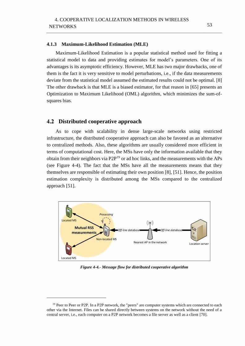
4. COOPERATIVE LOCALIZATION METHODS IN WIRELESS
NETWORKS 53
4.1.3 Maximum-Likelihood Estimation (MLE)
Maximum-Likelihood Estimation is a popular statistical method used for fitting a
statistical model to data and providing estimates for model’s parameters. One of its
advantages is its asymptotic efficiency. However, MLE has two major drawbacks, one of
them is the fact it is very sensitive to model perturbations, i.e., if the data measurements
deviate from the statistical model assumed the estimated results could not be optimal. [8]
The other drawback is that MLE is a biased estimator, for that reason in [65] presents an
Optimization to Maximum Likelihood (OML) algorithm, which minimizes the sum-of-
squares bias.
Distributed cooperative approach
As to cope with scalability in dense large-scale networks using restricted
infrastructure, the distributed cooperative approach can also be favored as an alternative
to centralized methods. Also, these algorithms are usually considered more efficient in
terms of computational cost. Here, the MSs have only the information available that they
obtain from their neighbors via P2P19 or ad hoc links, and the measurements with the APs
(see Figure 4-4). The fact that the MSs have all the measurements means that they
themselves are responsible of estimating their own position [8], [51]. Hence, the position
estimation complexity is distributed among the MSs compared to the centralized
approach [51].
Non-located MS
Located MS
Located MS
Mutual RSS measurements
Nearest AP in the network
Off-line database Off-line database
Location server
Processing
Figure 4-4.- Message flow for distributed cooperative algorithm
19 Peer to Peer or P2P. In a P2P network, the "peers" are computer systems which are connected to each
other via the Internet. Files can be shared directly between systems on the network without the need of a
central server, i.e., each computer on a P2P network becomes a file server as well as a client [70].
4. COOPERATIVE LOCALIZATION METHODS IN WIRELESS
NETWORKS 54
On the other hand, distributed algorithms have lower accuracy compared to those
achieved with a centralized algorithm, due to the fact that calculus is done at the MSs,
where computational restrictions are present in order to avoid notorious battery
consumptions [8].
Three distributed methods are present in distributed algorithms: lateration, Bayesian
and non-Bayesian. Bayesian approaches consider MS coordinates (𝑥𝑀𝑆, 𝑦𝑀𝑆, 𝑧𝑀𝑆) as a
realization of a random variable with a priori PDF, while non-Bayesian and lateration
approaches consider (𝑥𝑀𝑆, 𝑦𝑀𝑆, 𝑧𝑀𝑆) as a deterministic variable [8].
4.2.1 Lateration
Lateration is based based on triangulation concept, but in this case the alteration
methods use the distances between the MSs and APs instead of using angles. This method
is known as trilateration if three nodes are used or multilateration when more than three
nodes are used [8].
Trilateration is classified as a distributed localization algorithm, which is range
based, i.e. it uses distance estimation to compute the position of MSs in a network with
the help of the received information from the APs, e.g.: RSS [66]. Using the estimated
distances obtained from neighbor MSs, non-located MS obtains their location estimating
the intersection point of the circles centered at the APs with the radius equal to estimated
distance (Figure 3-4). Hence, this technique is significantly affected by the presence of
errors in the RSS measurements.
4.2.2 Nonparametric Belief Propagation (NBP)
The belief propagation (BP) is a popular technique for estimating the marginal
probabilities of each of the variables. BP follows a message-passing formulation, in which
at each iteration every variable passes a message to its neighboring factors, and factors to
their neighboring variables. When the variables take a finite number of values, the
messages may be represented as vectors [67].
Non-parametric belief propagation (NBP), also known as Sum-Product Algorithm
(SPA) [52], is an inference algorithm for graphical models containing continuous,
possibly non-Gaussian random variables. NBP extends the popular class of particle
filtering algorithms20, which assume variables are related by a Markov chain, to general
graphs. Such sample-based representations are particularly useful in high-dimensional
20 Particle filtering, also known as Sequential Monte Carlo (SMC) methodology, generate discrete
random measures that can be naturally used to approximate integrals with respect to the posterior
distribution given the data (including, e.g., its mean) [71].
4. COOPERATIVE LOCALIZATION METHODS IN WIRELESS
NETWORKS 55
spaces, where discretization becomes computationally difficult. In NBP, messages are
represented by collections of weighted samples, smoothed by a Gaussian shape i.e.,
Gaussian mixtures [67].
4.2.3 Non-Bayesian Estimators
Based on [52] and [55], MLE and least squares estimation (LSE) are classified as a
non-Bayesian estimators and the basic idea of both estimators is to minimize a cost
function. First of all, the MSs broadcast their own coordinates to their neighbors, then
each MS estimates the mutual distance to each MS using, e.g., the RSS from the APs.
Finally, the MSs recalculate their own position using the RSS and the mutual distance
between MSs. All these steps are repeated until the algorithm converges [8].
The drawback of this method is the possibility that the algorithm does not converge
to a global minimum, which is caused by the bad selection of a starting point and which
affects the global accuracy of the algorithm, for that reason the initial point has to be
selected carefully when the algorithm is designed [8].
LSE only minimize the norm of the difference between the RSS and the distance
estimation, however, MLE exploits the knowledge of the noise statistics of the RSS
measurements [55].
Proposed cooperative approach
The cooperative approach proposed in this thesis, to corroborate the position
enhancement by the cooperative methods, is classified as a distributed algorithm, which
will be based on RSS based localization methods, such as FP and PL.
As was explained in section 3.3, the RSS based positioning involves two stages: the
training phase and the estimation phase. In order to create the corresponding training
database, the off-line measurements are required. With the database and the on-line
measurements, the cost function of the RSS positioning method adopted (FP or PL) can
be defined. Afterwards the joint cost function of all the MSs can be optimized.
Figure 4-5 describes more exhaustively the concept of proposed cooperative
algorithm procedure. Once the training phase has been performed and the off-line data
has been collected (as depicted by the wider light blue arrow located on the left side of
the figure), the MSs begin to collect the on-line data from all the APs (as depicted by the
red and green thin arrows located on the left side of the figure) and subsequently send
them to the location server by the nearest APs (as depicted by the wider red and green
arrows located on the down-left side of the figure). The location server will process the
on-line and off-line data applying a RSS-based localization method, such as FP or PL.
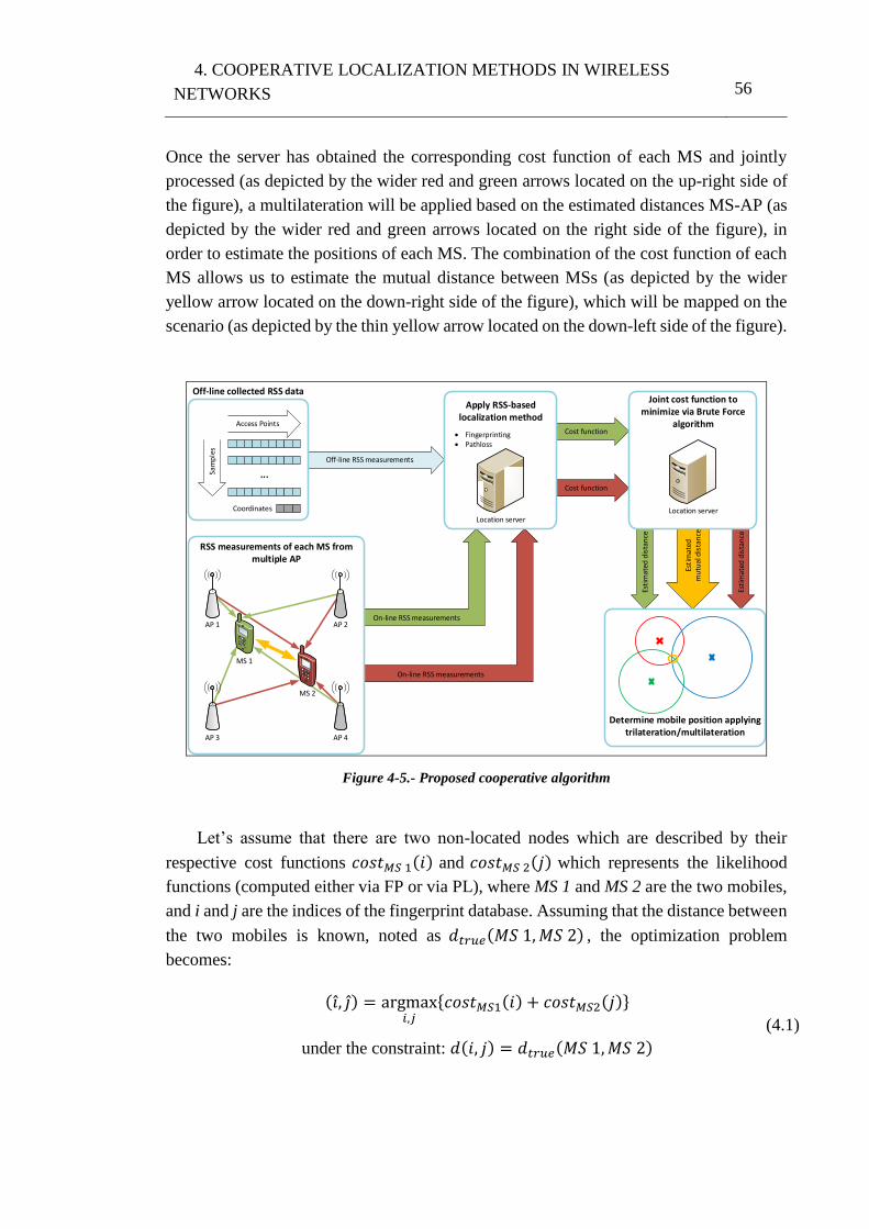
4. COOPERATIVE LOCALIZATION METHODS IN WIRELESS
NETWORKS 56
Once the server has obtained the corresponding cost function of each MS and jointly
processed (as depicted by the wider red and green arrows located on the up-right side of
the figure), a multilateration will be applied based on the estimated distances MS-AP (as
depicted by the wider red and green arrows located on the right side of the figure), in
order to estimate the positions of each MS. The combination of the cost function of each
MS allows us to estimate the mutual distance between MSs (as depicted by the wider
yellow arrow located on the down-right side of the figure), which will be mapped on the
scenario (as depicted by the thin yellow arrow located on the down-left side of the figure).
On-line RSS measurements
On-line RSS measurements
Esti
mat
ed
mu
tual
dis
tan
ce
Esti
mat
ed d
ista
nce
Esti
mat
ed d
ista
nce
Cost function
Cost function
Off-line RSS measurements
Determine mobile position applying trilateration/multilateration
···Sam
ple
s
Access Points
Coordinates
Off-line collected RSS data
RSS measurements of each MS from multiple AP
AP 3
AP 1 AP 2
AP 4
MS 2
MS 1
Location server
Apply RSS-based localization method
Fingerprinting Pathloss
Joint cost function to minimize via Brute Force
algorithm
Location server
Figure 4-5.- Proposed cooperative algorithm
Let’s assume that there are two non-located nodes which are described by their
respective cost functions 𝑐𝑜𝑠𝑡𝑀𝑆 1(𝑖) and 𝑐𝑜𝑠𝑡𝑀𝑆 2(𝑗) which represents the likelihood
functions (computed either via FP or via PL), where MS 1 and MS 2 are the two mobiles,
and i and j are the indices of the fingerprint database. Assuming that the distance between
the two mobiles is known, noted as 𝑑𝑡𝑟𝑢𝑒(𝑀𝑆 1,𝑀𝑆 2) , the optimization problem
becomes:
(𝑖̂, 𝑗̂) = argmax𝑖,𝑗
{𝑐𝑜𝑠𝑡𝑀𝑆1(𝑖) + 𝑐𝑜𝑠𝑡𝑀𝑆2(𝑗)}
under the constraint: 𝑑(𝑖, 𝑗) = 𝑑𝑡𝑟𝑢𝑒(𝑀𝑆 1,𝑀𝑆 2)
(4.1)
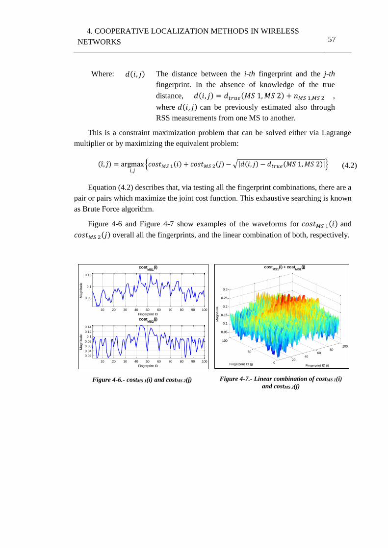
4. COOPERATIVE LOCALIZATION METHODS IN WIRELESS
NETWORKS 57
Where: 𝑑(𝑖, 𝑗) The distance between the i-th fingerprint and the j-th
fingerprint. In the absence of knowledge of the true
distance, 𝑑(𝑖, 𝑗) = 𝑑𝑡𝑟𝑢𝑒(𝑀𝑆 1,𝑀𝑆 2) + 𝑛𝑀𝑆 1,𝑀𝑆 2 ,
where 𝑑(𝑖, 𝑗) can be previously estimated also through
RSS measurements from one MS to another.
This is a constraint maximization problem that can be solved either via Lagrange
multiplier or by maximizing the equivalent problem:
(𝑖̂, 𝑗̂) = argmax𝑖,𝑗
{𝑐𝑜𝑠𝑡𝑀𝑆 1(𝑖) + 𝑐𝑜𝑠𝑡𝑀𝑆 2(𝑗) − √|𝑑(𝑖, 𝑗) − 𝑑𝑡𝑟𝑢𝑒(𝑀𝑆 1,𝑀𝑆 2)|} (4.2)
Equation (4.2) describes that, via testing all the fingerprint combinations, there are a
pair or pairs which maximize the joint cost function. This exhaustive searching is known
as Brute Force algorithm.
Figure 4-6 and Figure 4-7 show examples of the waveforms for 𝑐𝑜𝑠𝑡𝑀𝑆 1(𝑖) and
𝑐𝑜𝑠𝑡𝑀𝑆 2(𝑗) overall all the fingerprints, and the linear combination of both, respectively.
Figure 4-6.- costMS 1(i) and costMS 2(j)
Figure 4-7.- Linear combination of costMS 1(i)
and costMS 2(j)
10 20 30 40 50 60 70 80 90 100
0.05
0.1
0.15
costMS1
(i)
Fingerprint ID
Magnitude
10 20 30 40 50 60 70 80 90 100
0.02
0.04
0.06
0.08
0.1
0.12
0.14
costMS2
(j)
Fingerprint ID
Magnitude
2040
6080
100
0
50
100
0.05
0.1
0.15
0.2
0.25
0.3
Fingerprint ID (i)
costMS1
(i) + costMS2
(j)
Fingerprint ID (j)
Magnitude
5 Investigated approaches and comparative results
This section analyzes the results of computer simulations and experiments that have
been performed by developing proof of concepts of both methods:
Non-cooperative methods framework based on simulation results
implemented in Matlab
o FP approach
o PL approach
Proposed cooperative approach based on simulation results implemented in
Matlab
Proposed cooperative approach based on experimental results, using real
devices in a WLAN, from different buildings. Those buildings are located in
Tampere – Finland, such as Tietotalo, Duo, Sahkotalo, Koskikeskus and
Hermia.
o Proposed cooperative approach
The average location accuracy is evaluated quantifying the Root Mean Squared Error
(RMSE) of the distance error, i.e., quantifying the difference between the true MS
location and the estimated one based on the distance error, noted as ε.
𝜀 = √(𝑥𝑀𝑆 − �̂�𝑀𝑆)2 + (𝑦𝑀𝑆 − �̂�𝑀𝑆)2 (5.1)
Where: (𝑥𝑀𝑆, 𝑦𝑀𝑆) The real location coordinates of the MS
(�̂�𝑀𝑆, �̂�𝑀𝑆) The estimated coordinates of the MS
Assuming that each MS performs a trajectory in a determined scenario, the RMSE is
quantified over all the samples acquired over the path described by the MS (or MS
tracking points 𝑁𝑇𝑃 ). To observe the performance of the algorithms under study, the
RMSE has to be evaluated for different levels of noise variance present in the scenario.
𝑅𝑀𝑆𝐸 = √1
𝑁𝑇𝑃∑{𝜀𝑛}2
𝑁𝑇𝑃
𝑛=1
(5.2)
Where: 𝜀𝑛 The distance error of the n-th tracking point
As was described in Chapter 3, the solution of each algorithm will be the NN value
or an average of NN. For that reason, the purpose of the RMSE merit figure is to allow
the comparison between both solutions for different levels of noise power. Also, this merit
5. INVESTIGATED APPROACHES AND COMPARATIVE RESULTS 59
figure allows us to perform the comparison between non-cooperative and cooperative
methods.
On the other hand, in the case of non-cooperative methods, in order to compare the
RMSE enhancement of all the approaches described before, a Monte Carlo21 technique
has to be applied to compute an averaged RMSE (𝑅𝑀𝑆𝐸̅̅ ̅̅ ̅̅ ̅̅ ) and observe the tendency of
this merit figure for different levels of noise power as well. For a given number of Monte
Carlo iteration or realization (𝑁𝑅), the averaged RMSE value of each non-cooperative
approach at each noise level is defined as:
𝑅𝑀𝑆𝐸̅̅ ̅̅ ̅̅ ̅̅ = √1
𝑁𝑅∑{
1
𝑁𝑇𝑃∑{𝜀𝑛
𝑖 }2
𝑁𝑇𝑃
𝑛=1
}
𝑁𝑅
𝑖=1
(5.3)
Where: 𝜀𝑛𝑖 The distance error of the n-th tracking point at the i-th Monte
Carlo realization
For each non-cooperative and cooperative approach, a simulator has been created. If
the simulator conditions are not specified, its default values are:
10000 m2 of area
16 APs
o Transmit power: 10 𝑑𝐵 ≤ 𝑃𝑇𝑋 ≤ 15𝑑𝐵
o Pathloss exponent: 1,2 ≤ 𝑛 ≤ 8
256 fingerprints
20 samples captured per RSS and summarized applying the arithmetic mean
estimator
3 MSs which perform a straight line trajectory with 50 tracking points
20 samples of shadowing standard deviation: 0𝑑𝐵 ≤ 𝜎2 ≤ 7𝑑𝐵
The next sections address the simulated approaches in this thesis. At the beginning
of each section, the simulator will be described using a block diagram in order to facilitate
its comprehension.
21 The Monte Carlo method is defined as representing the solution of a problem as a parameter of a
hypothetical population, and using a random sequence of numbers to construct a sample of the population,
from which statistical estimates of the parameter can be obtained. Monte Carlo method can be applied to a
given problem that does not depend on the stochastic nature of the system being studied, but only on our
ability to formulate the problem in such a way that random numbers may be used to obtain the solution
[72].
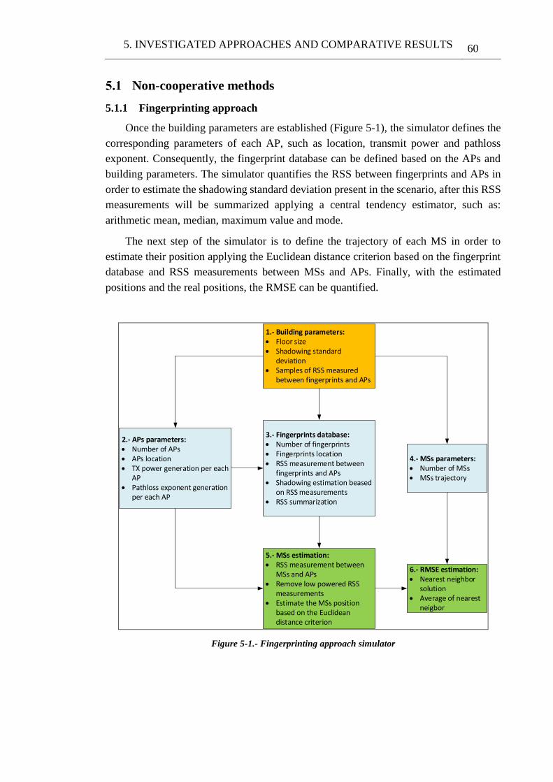
5. INVESTIGATED APPROACHES AND COMPARATIVE RESULTS 60
Non-cooperative methods
5.1.1 Fingerprinting approach
Once the building parameters are established (Figure 5-1), the simulator defines the
corresponding parameters of each AP, such as location, transmit power and pathloss
exponent. Consequently, the fingerprint database can be defined based on the APs and
building parameters. The simulator quantifies the RSS between fingerprints and APs in
order to estimate the shadowing standard deviation present in the scenario, after this RSS
measurements will be summarized applying a central tendency estimator, such as:
arithmetic mean, median, maximum value and mode.
The next step of the simulator is to define the trajectory of each MS in order to
estimate their position applying the Euclidean distance criterion based on the fingerprint
database and RSS measurements between MSs and APs. Finally, with the estimated
positions and the real positions, the RMSE can be quantified.
1.- Building parameters: Floor size Shadowing standard
deviation Samples of RSS measured
between fingerprints and APs
2.- APs parameters: Number of APs APs location TX power generation per each
AP Pathloss exponent generation
per each AP
3.- Fingerprints database: Number of fingerprints Fingerprints location RSS measurement between
fingerprints and APs Shadowing estimation beased
on RSS measurements RSS summarization
4.- MSs parameters: Number of MSs MSs trajectory
5.- MSs estimation: RSS measurement between
MSs and APs Remove low powered RSS
measurements Estimate the MSs position
based on the Euclidean distance criterion
6.- RMSE estimation: Nearest neighbor
solution Average of nearest
neigbor
Figure 5-1.- Fingerprinting approach simulator
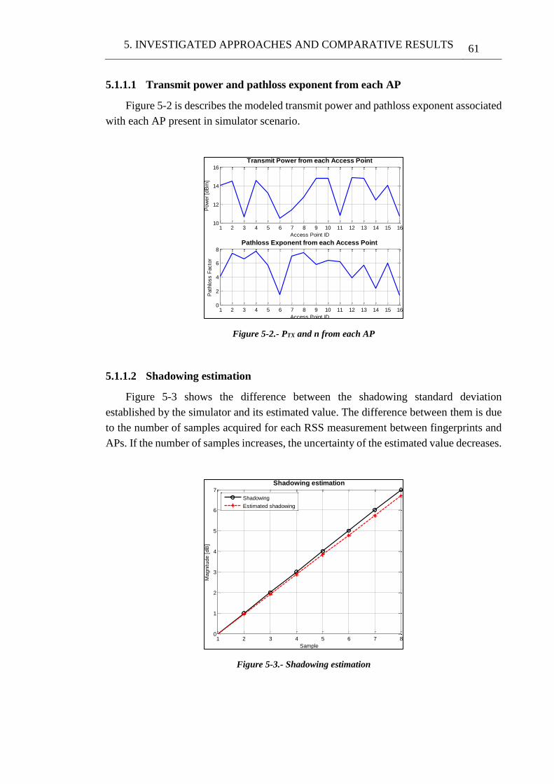
5. INVESTIGATED APPROACHES AND COMPARATIVE RESULTS 61
5.1.1.1 Transmit power and pathloss exponent from each AP
Figure 5-2 is describes the modeled transmit power and pathloss exponent associated
with each AP present in simulator scenario.
Figure 5-2.- PTX and n from each AP
5.1.1.2 Shadowing estimation
Figure 5-3 shows the difference between the shadowing standard deviation
established by the simulator and its estimated value. The difference between them is due
to the number of samples acquired for each RSS measurement between fingerprints and
APs. If the number of samples increases, the uncertainty of the estimated value decreases.
Figure 5-3.- Shadowing estimation
1 2 3 4 5 6 7 8 9 10 11 12 13 14 15 1610
12
14
16
Access Point ID
Pow
er
[dB
m]
Transmit Power from each Access Point
1 2 3 4 5 6 7 8 9 10 11 12 13 14 15 160
2
4
6
8
Access Point ID
Path
loss F
acto
r
Pathloss Exponent from each Access Point
1 2 3 4 5 6 7 80
1
2
3
4
5
6
7
Sample
Magnitude [
dB
]
Shadowing estimation
Shadowing
Estimated shadowing
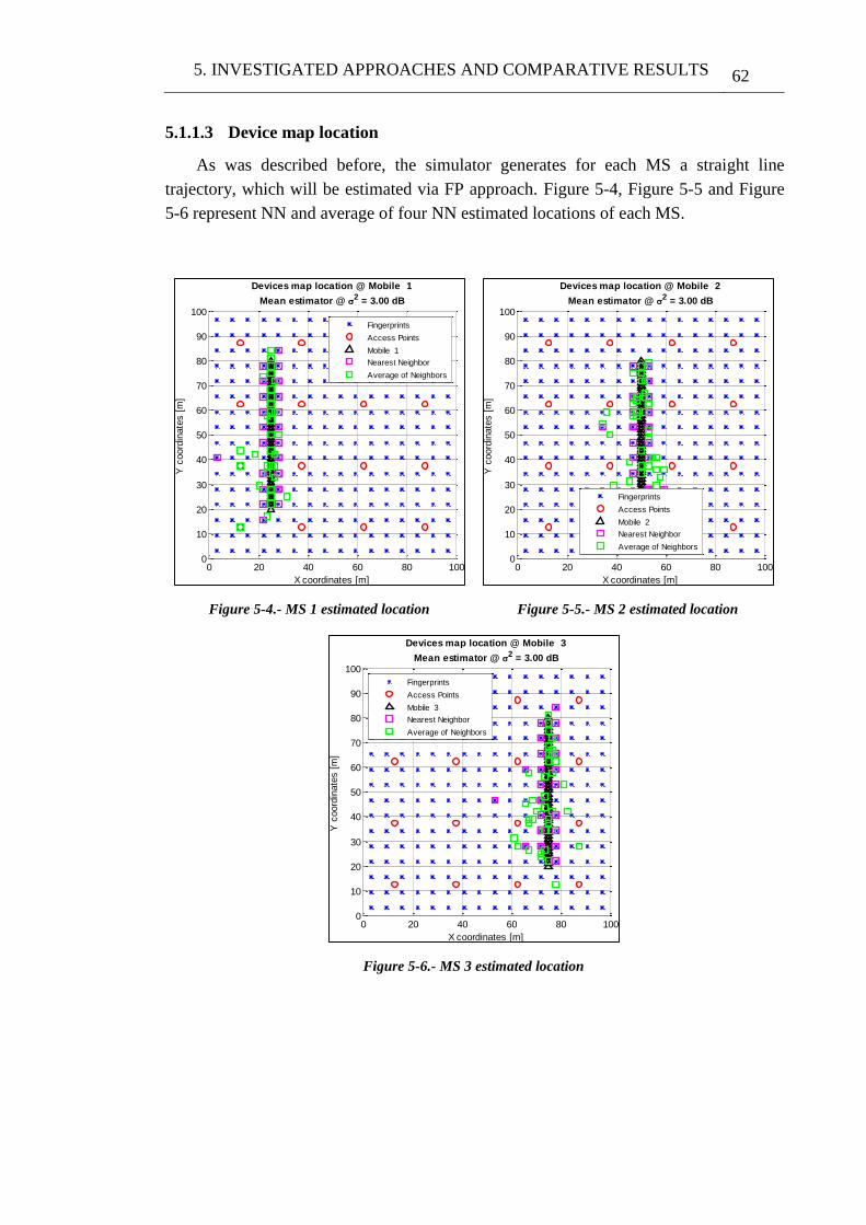
5. INVESTIGATED APPROACHES AND COMPARATIVE RESULTS 62
5.1.1.3 Device map location
As was described before, the simulator generates for each MS a straight line
trajectory, which will be estimated via FP approach. Figure 5-4, Figure 5-5 and Figure
5-6 represent NN and average of four NN estimated locations of each MS.
Figure 5-4.- MS 1 estimated location
Figure 5-5.- MS 2 estimated location
Figure 5-6.- MS 3 estimated location
0 20 40 60 80 1000
10
20
30
40
50
60
70
80
90
100
Devices map location @ Mobile 1
Mean estimator @ 2 = 3.00 dB
X coordinates [m]
Y c
oord
inate
s [
m]
Fingerprints
Access Points
Mobile 1
Nearest Neighbor
Average of Neighbors
0 20 40 60 80 1000
10
20
30
40
50
60
70
80
90
100
Devices map location @ Mobile 2
Mean estimator @ 2 = 3.00 dB
X coordinates [m]
Y c
oord
inate
s [
m]
Fingerprints
Access Points
Mobile 2
Nearest Neighbor
Average of Neighbors
0 20 40 60 80 1000
10
20
30
40
50
60
70
80
90
100
Devices map location @ Mobile 3
Mean estimator @ 2 = 3.00 dB
X coordinates [m]
Y c
oord
inate
s [
m]
Fingerprints
Access Points
Mobile 3
Nearest Neighbor
Average of Neighbors
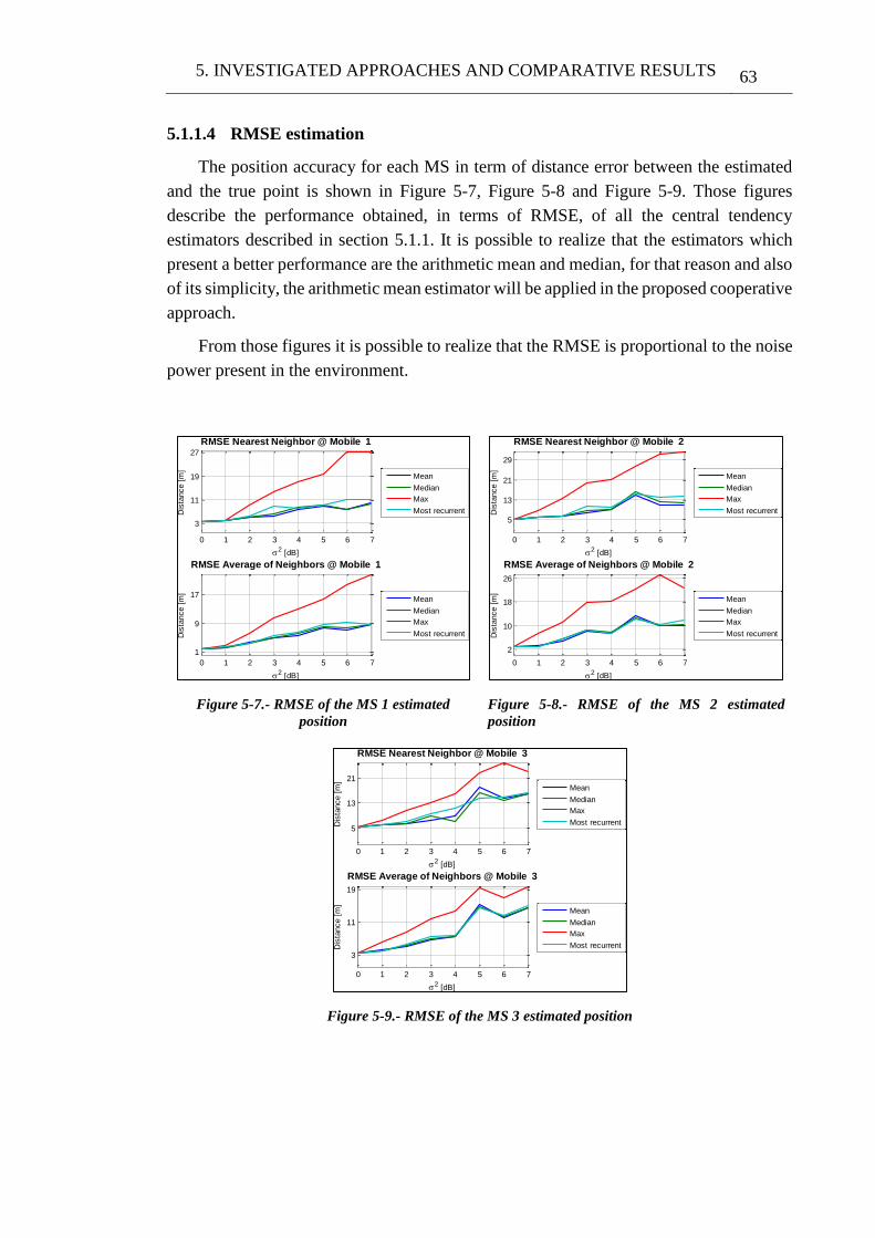
5. INVESTIGATED APPROACHES AND COMPARATIVE RESULTS 63
5.1.1.4 RMSE estimation
The position accuracy for each MS in term of distance error between the estimated
and the true point is shown in Figure 5-7, Figure 5-8 and Figure 5-9. Those figures
describe the performance obtained, in terms of RMSE, of all the central tendency
estimators described in section 5.1.1. It is possible to realize that the estimators which
present a better performance are the arithmetic mean and median, for that reason and also
of its simplicity, the arithmetic mean estimator will be applied in the proposed cooperative
approach.
From those figures it is possible to realize that the RMSE is proportional to the noise
power present in the environment.
Figure 5-7.- RMSE of the MS 1 estimated
position
Figure 5-8.- RMSE of the MS 2 estimated
position
Figure 5-9.- RMSE of the MS 3 estimated position
0 1 2 3 4 5 6 7
3
11
19
27
2 [dB]
Dis
tance [
m]
RMSE Nearest Neighbor @ Mobile 1
Mean
Median
Max
Most recurrent
0 1 2 3 4 5 6 7
1
9
17
2 [dB]
Dis
tance [
m]
RMSE Average of Neighbors @ Mobile 1
Mean
Median
Max
Most recurrent
0 1 2 3 4 5 6 7
5
13
21
29
2 [dB]
Dis
tance [
m]
RMSE Nearest Neighbor @ Mobile 2
Mean
Median
Max
Most recurrent
0 1 2 3 4 5 6 7
2
10
18
26
2 [dB]
Dis
tance [
m]
RMSE Average of Neighbors @ Mobile 2
Mean
Median
Max
Most recurrent
0 1 2 3 4 5 6 7
5
13
21
2 [dB]
Dis
tance [
m]
RMSE Nearest Neighbor @ Mobile 3
Mean
Median
Max
Most recurrent
0 1 2 3 4 5 6 7
3
11
19
2 [dB]
Dis
tance [
m]
RMSE Average of Neighbors @ Mobile 3
Mean
Median
Max
Most recurrent
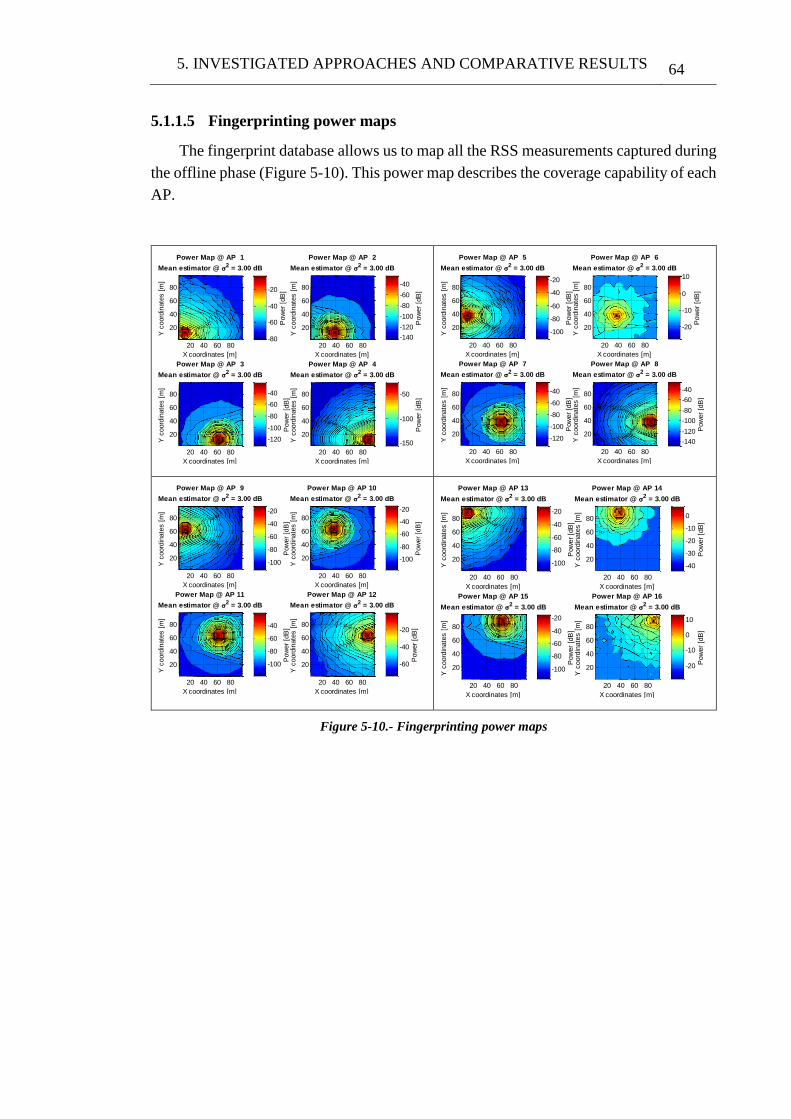
5. INVESTIGATED APPROACHES AND COMPARATIVE RESULTS 64
5.1.1.5 Fingerprinting power maps
The fingerprint database allows us to map all the RSS measurements captured during
the offline phase (Figure 5-10). This power map describes the coverage capability of each
AP.
Figure 5-10.- Fingerprinting power maps
X coordinates [m]
Y c
oord
inate
s [
m]
Power Map @ AP 1
Mean estimator @ 2 = 3.00 dB
20 40 60 80
20
40
60
80P
ow
er
[dB
]
-80
-60
-40
-20
X coordinates [m]
Y c
oord
inate
s [
m]
Power Map @ AP 2
Mean estimator @ 2 = 3.00 dB
20 40 60 80
20
40
60
80
Pow
er
[dB
]
-140
-120
-100
-80
-60
-40
X coordinates [m]
Y c
oord
inate
s [
m]
Power Map @ AP 3
Mean estimator @ 2 = 3.00 dB
20 40 60 80
20
40
60
80
Pow
er
[dB
]
-120
-100
-80
-60
-40
X coordinates [m]
Y c
oord
inate
s [
m]
Power Map @ AP 4
Mean estimator @ 2 = 3.00 dB
20 40 60 80
20
40
60
80
Pow
er
[dB
]
-150
-100
-50
X coordinates [m]
Y c
oord
inate
s [
m]
Power Map @ AP 5
Mean estimator @ 2 = 3.00 dB
20 40 60 80
20
40
60
80
Pow
er
[dB
]
-100
-80
-60
-40
-20
X coordinates [m]
Y c
oord
inate
s [
m]
Power Map @ AP 6
Mean estimator @ 2 = 3.00 dB
20 40 60 80
20
40
60
80
Pow
er
[dB
]
-20
-10
0
10
X coordinates [m]
Y c
oord
inate
s [
m]
Power Map @ AP 7
Mean estimator @ 2 = 3.00 dB
20 40 60 80
20
40
60
80
Pow
er
[dB
]
-120
-100
-80
-60
-40
X coordinates [m]
Y c
oord
inate
s [
m]
Power Map @ AP 8
Mean estimator @ 2 = 3.00 dB
20 40 60 80
20
40
60
80
Pow
er
[dB
]
-140
-120
-100
-80
-60
-40
X coordinates [m]
Y c
oord
inate
s [
m]
Power Map @ AP 9
Mean estimator @ 2 = 3.00 dB
20 40 60 80
20
40
60
80
Pow
er
[dB
]
-100
-80
-60
-40
-20
X coordinates [m]
Y c
oord
inate
s [
m]
Power Map @ AP 10
Mean estimator @ 2 = 3.00 dB
20 40 60 80
20
40
60
80
Pow
er
[dB
]
-100
-80
-60
-40
-20
X coordinates [m]
Y c
oord
inate
s [
m]
Power Map @ AP 11
Mean estimator @ 2 = 3.00 dB
20 40 60 80
20
40
60
80
Pow
er
[dB
]
-100
-80
-60
-40
X coordinates [m]
Y c
oord
inate
s [
m]
Power Map @ AP 12
Mean estimator @ 2 = 3.00 dB
20 40 60 80
20
40
60
80
Pow
er
[dB
]
-60
-40
-20
X coordinates [m]
Y c
oord
inate
s [
m]
Power Map @ AP 13
Mean estimator @ 2 = 3.00 dB
20 40 60 80
20
40
60
80
Pow
er
[dB
]-100
-80
-60
-40
-20
X coordinates [m]
Y c
oord
inate
s [
m]
Power Map @ AP 14
Mean estimator @ 2 = 3.00 dB
20 40 60 80
20
40
60
80
Pow
er
[dB
]
-40
-30
-20
-10
0
X coordinates [m]
Y c
oord
inate
s [
m]
Power Map @ AP 15
Mean estimator @ 2 = 3.00 dB
20 40 60 80
20
40
60
80
Pow
er
[dB
]
-100
-80
-60
-40
-20
X coordinates [m]
Y c
oord
inate
s [
m]
Power Map @ AP 16
Mean estimator @ 2 = 3.00 dB
20 40 60 80
20
40
60
80
Pow
er
[dB
]
-20
-10
0
10
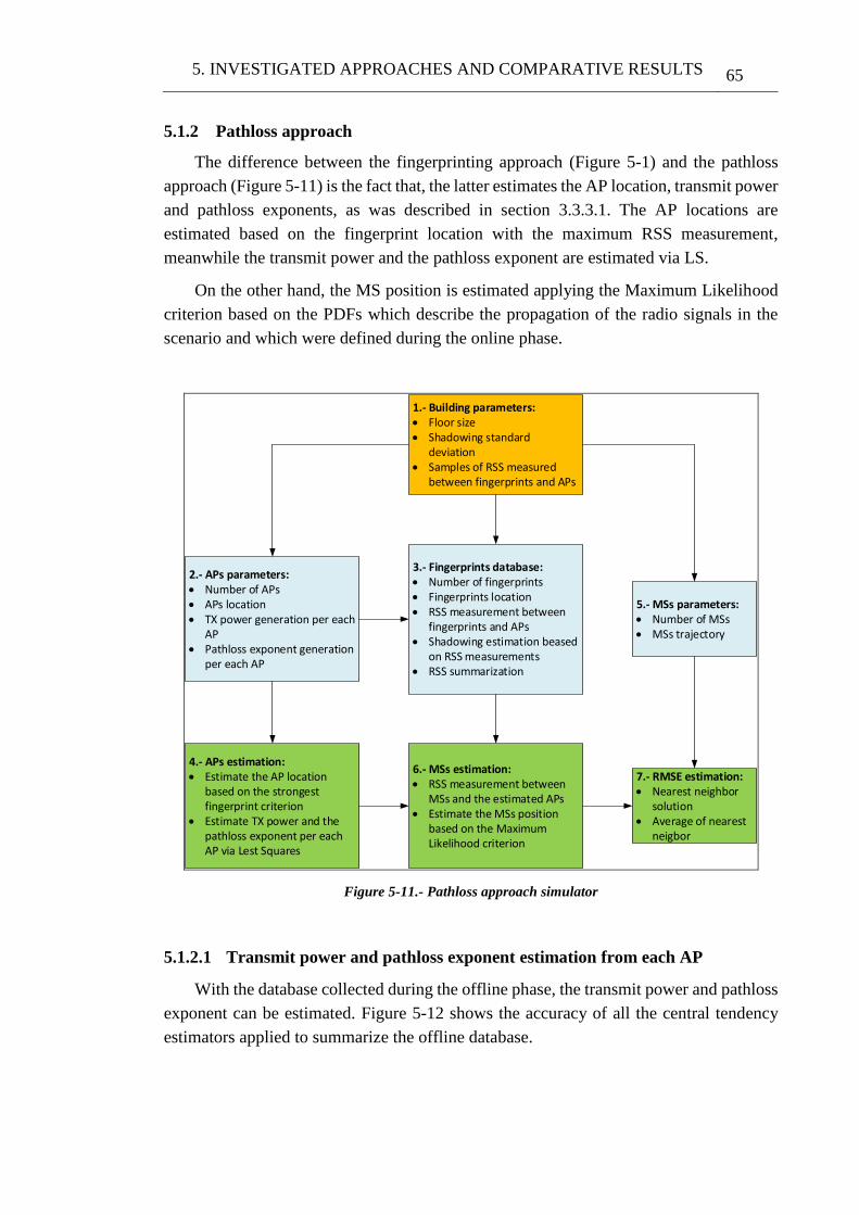
5. INVESTIGATED APPROACHES AND COMPARATIVE RESULTS 65
5.1.2 Pathloss approach
The difference between the fingerprinting approach (Figure 5-1) and the pathloss
approach (Figure 5-11) is the fact that, the latter estimates the AP location, transmit power
and pathloss exponents, as was described in section 3.3.3.1. The AP locations are
estimated based on the fingerprint location with the maximum RSS measurement,
meanwhile the transmit power and the pathloss exponent are estimated via LS.
On the other hand, the MS position is estimated applying the Maximum Likelihood
criterion based on the PDFs which describe the propagation of the radio signals in the
scenario and which were defined during the online phase.
1.- Building parameters: Floor size Shadowing standard
deviation Samples of RSS measured
between fingerprints and APs
2.- APs parameters: Number of APs APs location TX power generation per each
AP Pathloss exponent generation
per each AP
3.- Fingerprints database: Number of fingerprints Fingerprints location RSS measurement between
fingerprints and APs Shadowing estimation beased
on RSS measurements RSS summarization
5.- MSs parameters: Number of MSs MSs trajectory
6.- MSs estimation: RSS measurement between
MSs and the estimated APs Estimate the MSs position
based on the Maximum Likelihood criterion
7.- RMSE estimation: Nearest neighbor
solution Average of nearest
neigbor
4.- APs estimation: Estimate the AP location
based on the strongest fingerprint criterion
Estimate TX power and the pathloss exponent per each AP via Lest Squares
Figure 5-11.- Pathloss approach simulator
5.1.2.1 Transmit power and pathloss exponent estimation from each AP
With the database collected during the offline phase, the transmit power and pathloss
exponent can be estimated. Figure 5-12 shows the accuracy of all the central tendency
estimators applied to summarize the offline database.
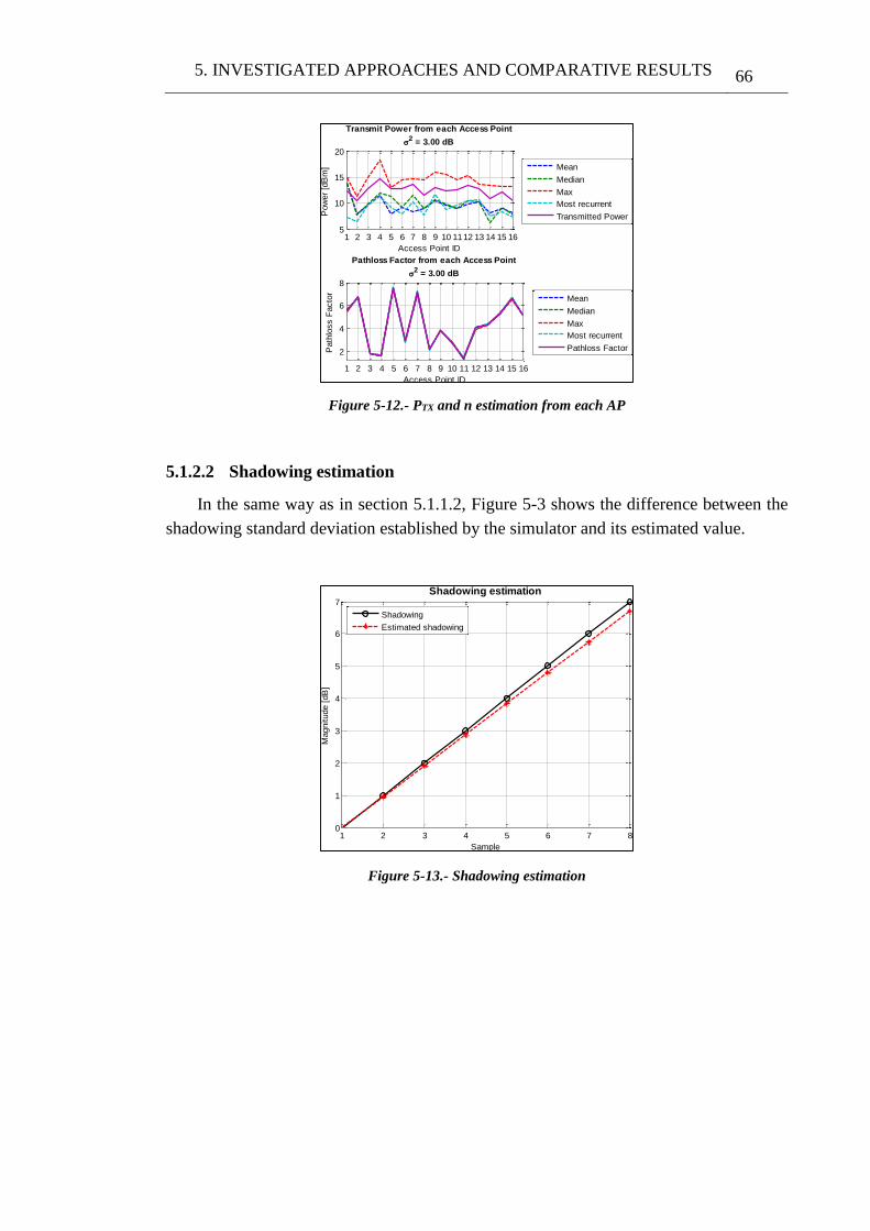
5. INVESTIGATED APPROACHES AND COMPARATIVE RESULTS 66
Figure 5-12.- PTX and n estimation from each AP
5.1.2.2 Shadowing estimation
In the same way as in section 5.1.1.2, Figure 5-3 shows the difference between the
shadowing standard deviation established by the simulator and its estimated value.
Figure 5-13.- Shadowing estimation
1 2 3 4 5 6 7 8 9 10 1112 13 14 15 165
10
15
20
Access Point ID
Pow
er
[dB
m]
Transmit Power from each Access Point
2 = 3.00 dB
Mean
Median
Max
Most recurrent
Transmitted Power
1 2 3 4 5 6 7 8 9 10 11 12 13 14 15 16
2
4
6
8
Access Point ID
Path
loss F
acto
r
Pathloss Factor from each Access Point
2 = 3.00 dB
Mean
Median
Max
Most recurrent
Pathloss Factor
1 2 3 4 5 6 7 80
1
2
3
4
5
6
7
Sample
Magnitude [
dB
]
Shadowing estimation
Shadowing
Estimated shadowing
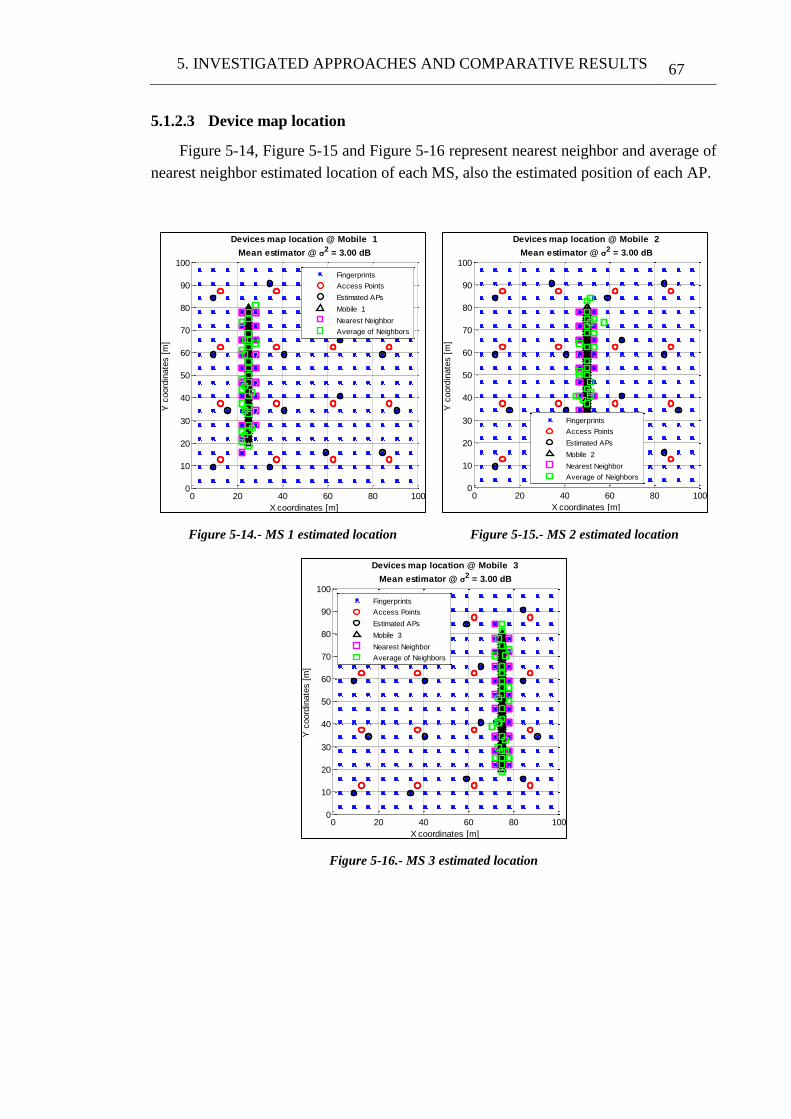
5. INVESTIGATED APPROACHES AND COMPARATIVE RESULTS 67
5.1.2.3 Device map location
Figure 5-14, Figure 5-15 and Figure 5-16 represent nearest neighbor and average of
nearest neighbor estimated location of each MS, also the estimated position of each AP.
Figure 5-14.- MS 1 estimated location
Figure 5-15.- MS 2 estimated location
Figure 5-16.- MS 3 estimated location
0 20 40 60 80 1000
10
20
30
40
50
60
70
80
90
100
Devices map location @ Mobile 1
Mean estimator @ 2 = 3.00 dB
X coordinates [m]
Y c
oord
inate
s [
m]
Fingerprints
Access Points
Estimated APs
Mobile 1
Nearest Neighbor
Average of Neighbors
0 20 40 60 80 1000
10
20
30
40
50
60
70
80
90
100
Devices map location @ Mobile 2
Mean estimator @ 2 = 3.00 dB
X coordinates [m]
Y c
oord
inate
s [
m]
Fingerprints
Access Points
Estimated APs
Mobile 2
Nearest Neighbor
Average of Neighbors
0 20 40 60 80 1000
10
20
30
40
50
60
70
80
90
100
Devices map location @ Mobile 3
Mean estimator @ 2 = 3.00 dB
X coordinates [m]
Y c
oord
inate
s [
m]
Fingerprints
Access Points
Estimated APs
Mobile 3
Nearest Neighbor
Average of Neighbors
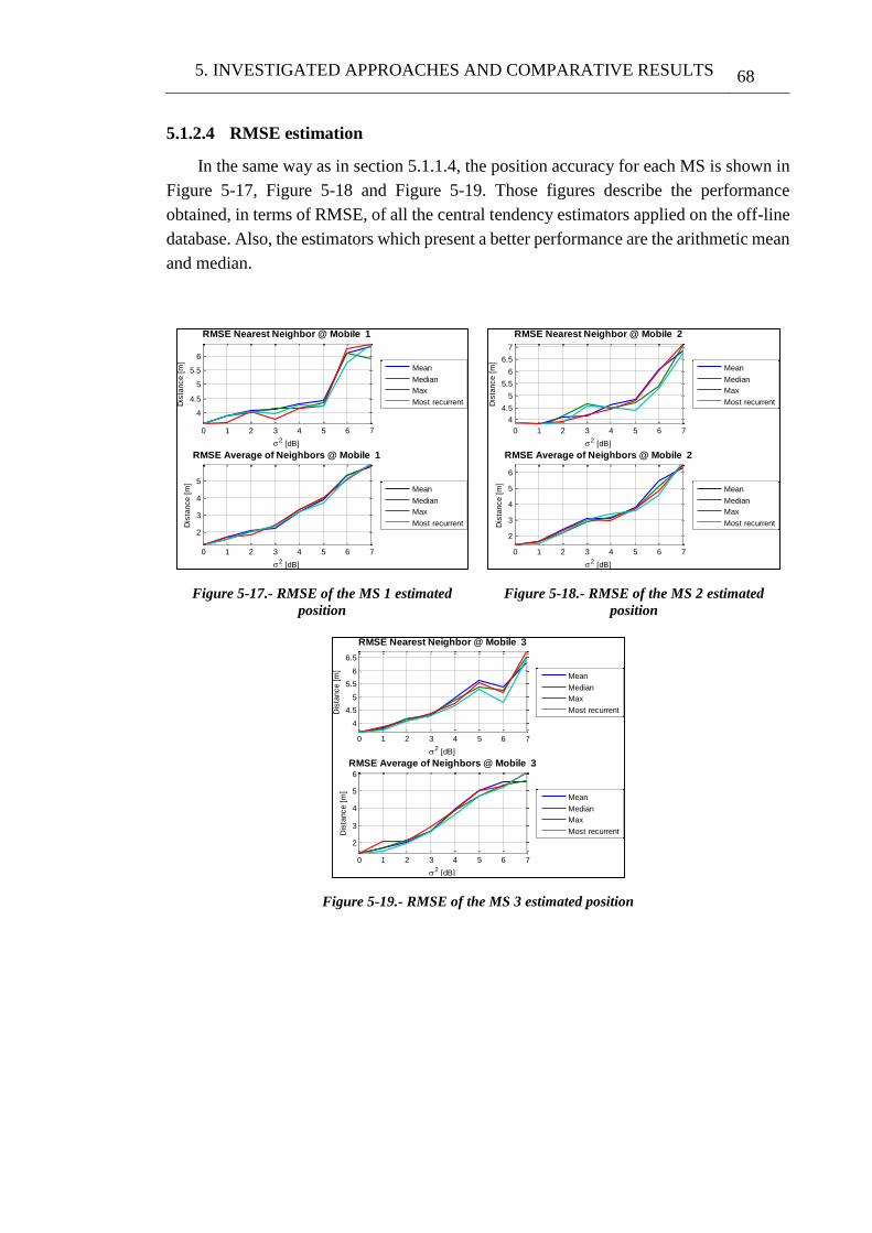
5. INVESTIGATED APPROACHES AND COMPARATIVE RESULTS 68
5.1.2.4 RMSE estimation
In the same way as in section 5.1.1.4, the position accuracy for each MS is shown in
Figure 5-17, Figure 5-18 and Figure 5-19. Those figures describe the performance
obtained, in terms of RMSE, of all the central tendency estimators applied on the off-line
database. Also, the estimators which present a better performance are the arithmetic mean
and median.
Figure 5-17.- RMSE of the MS 1 estimated
position
Figure 5-18.- RMSE of the MS 2 estimated
position
Figure 5-19.- RMSE of the MS 3 estimated position
0 1 2 3 4 5 6 7
4
4.5
5
5.5
6
2 [dB]
Dis
tance [
m]
RMSE Nearest Neighbor @ Mobile 1
Mean
Median
Max
Most recurrent
0 1 2 3 4 5 6 7
2
3
4
5
2 [dB]
Dis
tance [
m]
RMSE Average of Neighbors @ Mobile 1
Mean
Median
Max
Most recurrent
0 1 2 3 4 5 6 7
4
4.5
5
5.5
6
6.5
7
2 [dB]
Dis
tance [
m]
RMSE Nearest Neighbor @ Mobile 2
Mean
Median
Max
Most recurrent
0 1 2 3 4 5 6 7
2
3
4
5
6
2 [dB]
Dis
tance [
m]
RMSE Average of Neighbors @ Mobile 2
Mean
Median
Max
Most recurrent
0 1 2 3 4 5 6 7
4
4.5
5
5.5
6
6.5
2 [dB]
Dis
tance [
m]
RMSE Nearest Neighbor @ Mobile 3
Mean
Median
Max
Most recurrent
0 1 2 3 4 5 6 7
2
3
4
5
6
2 [dB]
Dis
tance [
m]
RMSE Average of Neighbors @ Mobile 3
Mean
Median
Max
Most recurrent
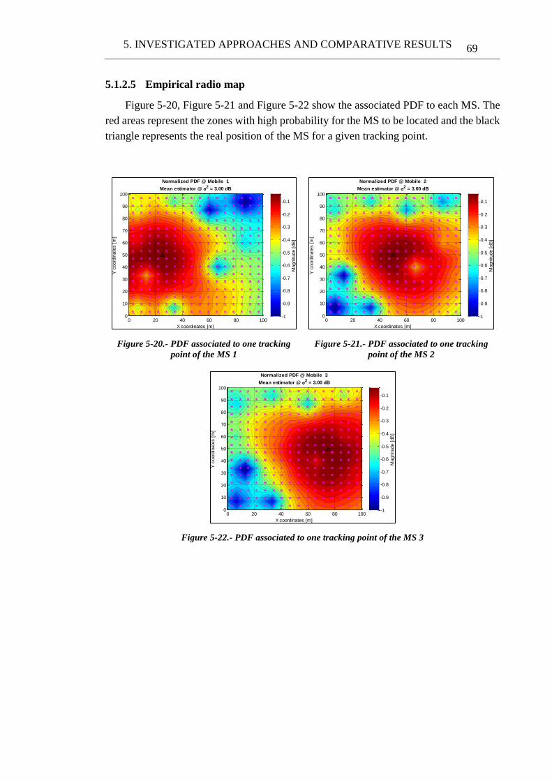
5. INVESTIGATED APPROACHES AND COMPARATIVE RESULTS 69
5.1.2.5 Empirical radio map
Figure 5-20, Figure 5-21 and Figure 5-22 show the associated PDF to each MS. The
red areas represent the zones with high probability for the MS to be located and the black
triangle represents the real position of the MS for a given tracking point.
Figure 5-20.- PDF associated to one tracking
point of the MS 1
Figure 5-21.- PDF associated to one tracking
point of the MS 2
Figure 5-22.- PDF associated to one tracking point of the MS 3
X coordinates [m]
Y c
oord
inate
s [
m]
Normalized PDF @ Mobile 1
Mean estimator @ 2 = 3.00 dB
0 20 40 60 80 1000
10
20
30
40
50
60
70
80
90
100
Magnitude [
dB
]
-1
-0.9
-0.8
-0.7
-0.6
-0.5
-0.4
-0.3
-0.2
-0.1
X coordinates [m]
Y c
oord
inate
s [
m]
Normalized PDF @ Mobile 2
Mean estimator @ 2 = 3.00 dB
0 20 40 60 80 1000
10
20
30
40
50
60
70
80
90
100
Magnitude [
dB
]
-1
-0.9
-0.8
-0.7
-0.6
-0.5
-0.4
-0.3
-0.2
-0.1
X coordinates [m]
Y c
oord
inate
s [
m]
Normalized PDF @ Mobile 3
Mean estimator @ 2 = 3.00 dB
0 20 40 60 80 1000
10
20
30
40
50
60
70
80
90
100M
agnitude [
dB
]
-1
-0.9
-0.8
-0.7
-0.6
-0.5
-0.4
-0.3
-0.2
-0.1
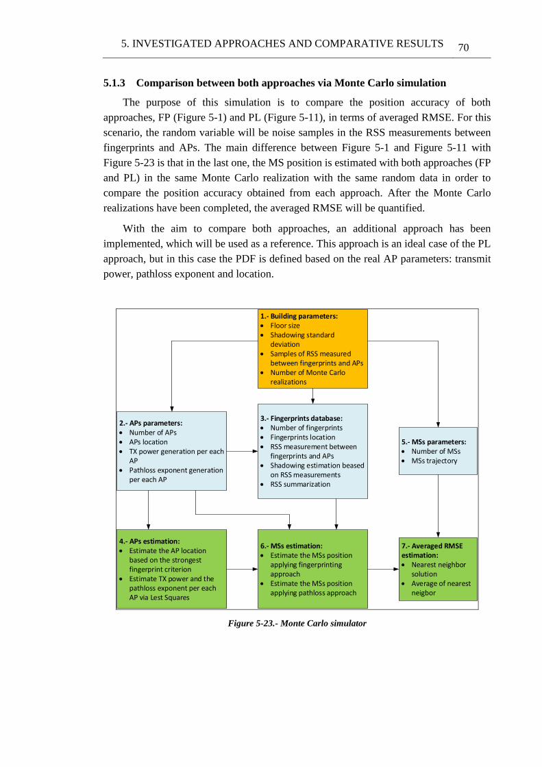
5. INVESTIGATED APPROACHES AND COMPARATIVE RESULTS 70
5.1.3 Comparison between both approaches via Monte Carlo simulation
The purpose of this simulation is to compare the position accuracy of both
approaches, FP (Figure 5-1) and PL (Figure 5-11), in terms of averaged RMSE. For this
scenario, the random variable will be noise samples in the RSS measurements between
fingerprints and APs. The main difference between Figure 5-1 and Figure 5-11 with
Figure 5-23 is that in the last one, the MS position is estimated with both approaches (FP
and PL) in the same Monte Carlo realization with the same random data in order to
compare the position accuracy obtained from each approach. After the Monte Carlo
realizations have been completed, the averaged RMSE will be quantified.
With the aim to compare both approaches, an additional approach has been
implemented, which will be used as a reference. This approach is an ideal case of the PL
approach, but in this case the PDF is defined based on the real AP parameters: transmit
power, pathloss exponent and location.
1.- Building parameters: Floor size Shadowing standard
deviation Samples of RSS measured
between fingerprints and APs Number of Monte Carlo
realizations
2.- APs parameters: Number of APs APs location TX power generation per each
AP Pathloss exponent generation
per each AP
3.- Fingerprints database: Number of fingerprints Fingerprints location RSS measurement between
fingerprints and APs Shadowing estimation beased
on RSS measurements RSS summarization
5.- MSs parameters: Number of MSs MSs trajectory
6.- MSs estimation: Estimate the MSs position
applying fingerprinting approach
Estimate the MSs position applying pathloss approach
7.- Averaged RMSE estimation: Nearest neighbor
solution Average of nearest
neigbor
4.- APs estimation: Estimate the AP location
based on the strongest fingerprint criterion
Estimate TX power and the pathloss exponent per each AP via Lest Squares
Figure 5-23.- Monte Carlo simulator
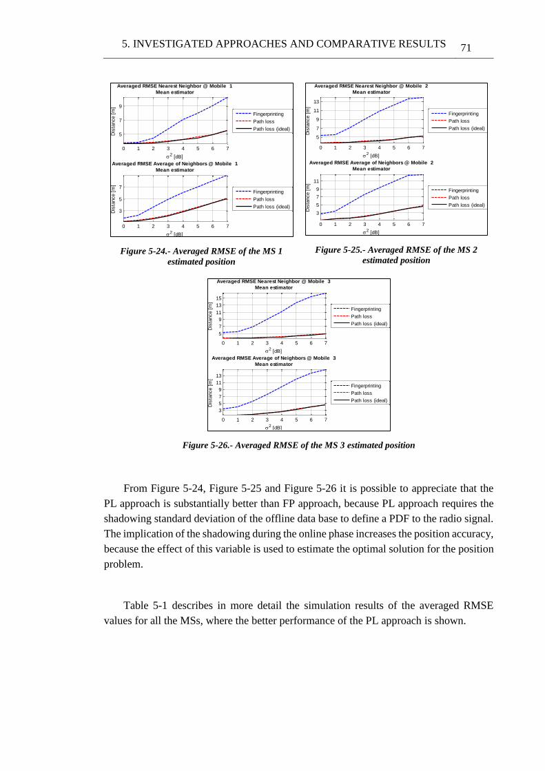
5. INVESTIGATED APPROACHES AND COMPARATIVE RESULTS 71
Figure 5-24.- Averaged RMSE of the MS 1
estimated position
Figure 5-25.- Averaged RMSE of the MS 2
estimated position
Figure 5-26.- Averaged RMSE of the MS 3 estimated position
From Figure 5-24, Figure 5-25 and Figure 5-26 it is possible to appreciate that the
PL approach is substantially better than FP approach, because PL approach requires the
shadowing standard deviation of the offline data base to define a PDF to the radio signal.
The implication of the shadowing during the online phase increases the position accuracy,
because the effect of this variable is used to estimate the optimal solution for the position
problem.
Table 5-1 describes in more detail the simulation results of the averaged RMSE
values for all the MSs, where the better performance of the PL approach is shown.
0 1 2 3 4 5 6 7
5
7
9
2 [dB]
Dis
tance [
m]
Averaged RMSE Nearest Neighbor @ Mobile 1
Mean estimator
Fingerprinting
Path loss
Path loss (ideal)
0 1 2 3 4 5 6 7
3
5
7
2 [dB]
Dis
tance [
m]
Averaged RMSE Average of Neighbors @ Mobile 1
Mean estimator
Fingerprinting
Path loss
Path loss (ideal)
0 1 2 3 4 5 6 7
5
7
9
11
13
2 [dB]
Dis
tance [
m]
Averaged RMSE Nearest Neighbor @ Mobile 2
Mean estimator
Fingerprinting
Path loss
Path loss (ideal)
0 1 2 3 4 5 6 7
3
5
7
9
11
2 [dB]
Dis
tance [
m]
Averaged RMSE Average of Neighbors @ Mobile 2
Mean estimator
Fingerprinting
Path loss
Path loss (ideal)
0 1 2 3 4 5 6 7
5
7
9
11
13
15
2 [dB]
Dis
tance [
m]
Averaged RMSE Nearest Neighbor @ Mobile 3
Mean estimator
Fingerprinting
Path loss
Path loss (ideal)
0 1 2 3 4 5 6 7
3
5
7
9
11
13
2 [dB]
Dis
tance [
m]
Averaged RMSE Average of Neighbors @ Mobile 3
Mean estimator
Fingerprinting
Path loss
Path loss (ideal)
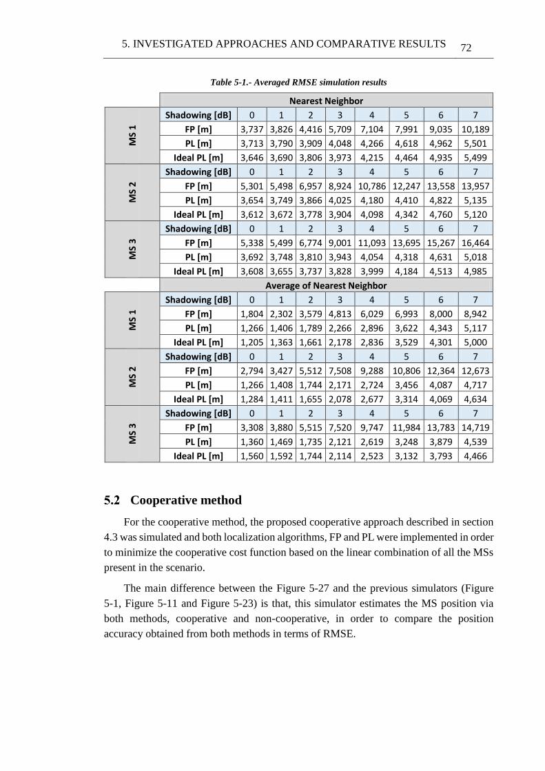
5. INVESTIGATED APPROACHES AND COMPARATIVE RESULTS 72
Table 5-1.- Averaged RMSE simulation results
Nearest Neighbor
MS
1
Shadowing [dB] 0 1 2 3 4 5 6 7
FP [m] 3,737 3,826 4,416 5,709 7,104 7,991 9,035 10,189
PL [m] 3,713 3,790 3,909 4,048 4,266 4,618 4,962 5,501
Ideal PL [m] 3,646 3,690 3,806 3,973 4,215 4,464 4,935 5,499
MS
2
Shadowing [dB] 0 1 2 3 4 5 6 7
FP [m] 5,301 5,498 6,957 8,924 10,786 12,247 13,558 13,957
PL [m] 3,654 3,749 3,866 4,025 4,180 4,410 4,822 5,135
Ideal PL [m] 3,612 3,672 3,778 3,904 4,098 4,342 4,760 5,120
MS
3
Shadowing [dB] 0 1 2 3 4 5 6 7
FP [m] 5,338 5,499 6,774 9,001 11,093 13,695 15,267 16,464
PL [m] 3,692 3,748 3,810 3,943 4,054 4,318 4,631 5,018
Ideal PL [m] 3,608 3,655 3,737 3,828 3,999 4,184 4,513 4,985
Average of Nearest Neighbor
MS
1
Shadowing [dB] 0 1 2 3 4 5 6 7
FP [m] 1,804 2,302 3,579 4,813 6,029 6,993 8,000 8,942
PL [m] 1,266 1,406 1,789 2,266 2,896 3,622 4,343 5,117
Ideal PL [m] 1,205 1,363 1,661 2,178 2,836 3,529 4,301 5,000
MS
2
Shadowing [dB] 0 1 2 3 4 5 6 7
FP [m] 2,794 3,427 5,512 7,508 9,288 10,806 12,364 12,673
PL [m] 1,266 1,408 1,744 2,171 2,724 3,456 4,087 4,717
Ideal PL [m] 1,284 1,411 1,655 2,078 2,677 3,314 4,069 4,634
MS
3
Shadowing [dB] 0 1 2 3 4 5 6 7
FP [m] 3,308 3,880 5,515 7,520 9,747 11,984 13,783 14,719
PL [m] 1,360 1,469 1,735 2,121 2,619 3,248 3,879 4,539
Ideal PL [m] 1,560 1,592 1,744 2,114 2,523 3,132 3,793 4,466
Cooperative method
For the cooperative method, the proposed cooperative approach described in section
4.3 was simulated and both localization algorithms, FP and PL were implemented in order
to minimize the cooperative cost function based on the linear combination of all the MSs
present in the scenario.
The main difference between the Figure 5-27 and the previous simulators (Figure
5-1, Figure 5-11 and Figure 5-23) is that, this simulator estimates the MS position via
both methods, cooperative and non-cooperative, in order to compare the position
accuracy obtained from both methods in terms of RMSE.
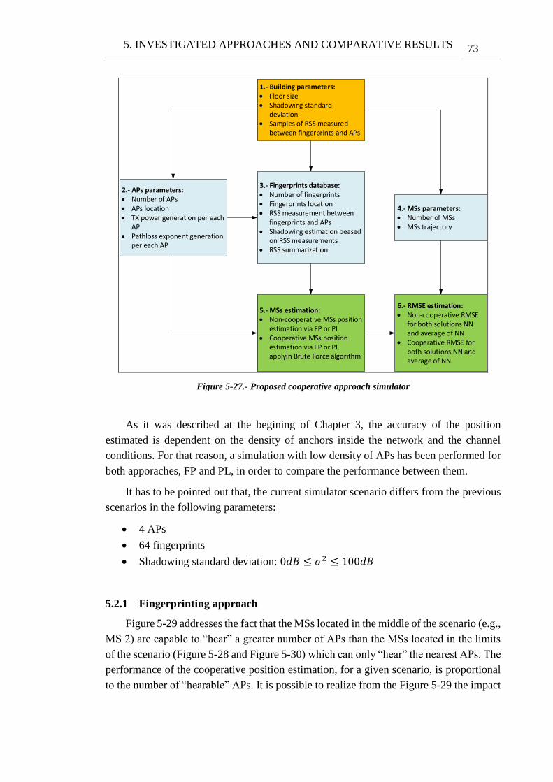
5. INVESTIGATED APPROACHES AND COMPARATIVE RESULTS 73
1.- Building parameters: Floor size Shadowing standard
deviation Samples of RSS measured
between fingerprints and APs
2.- APs parameters: Number of APs APs location TX power generation per each
AP Pathloss exponent generation
per each AP
3.- Fingerprints database: Number of fingerprints Fingerprints location RSS measurement between
fingerprints and APs Shadowing estimation beased
on RSS measurements RSS summarization
4.- MSs parameters: Number of MSs MSs trajectory
5.- MSs estimation: Non-cooperative MSs position
estimation via FP or PL Cooperative MSs position
estimation via FP or PL applyin Brute Force algorithm
6.- RMSE estimation: Non-cooperative RMSE
for both solutions NN and average of NN
Cooperative RMSE for both solutions NN and average of NN
Figure 5-27.- Proposed cooperative approach simulator
As it was described at the begining of Chapter 3, the accuracy of the position
estimated is dependent on the density of anchors inside the network and the channel
conditions. For that reason, a simulation with low density of APs has been performed for
both apporaches, FP and PL, in order to compare the performance between them.
It has to be pointed out that, the current simulator scenario differs from the previous
scenarios in the following parameters:
4 APs
64 fingerprints
Shadowing standard deviation: 0𝑑𝐵 ≤ 𝜎2 ≤ 100𝑑𝐵
5.2.1 Fingerprinting approach
Figure 5-29 addresses the fact that the MSs located in the middle of the scenario (e.g.,
MS 2) are capable to “hear” a greater number of APs than the MSs located in the limits
of the scenario (Figure 5-28 and Figure 5-30) which can only “hear” the nearest APs. The
performance of the cooperative position estimation, for a given scenario, is proportional
to the number of “hearable” APs. It is possible to realize from the Figure 5-29 the impact
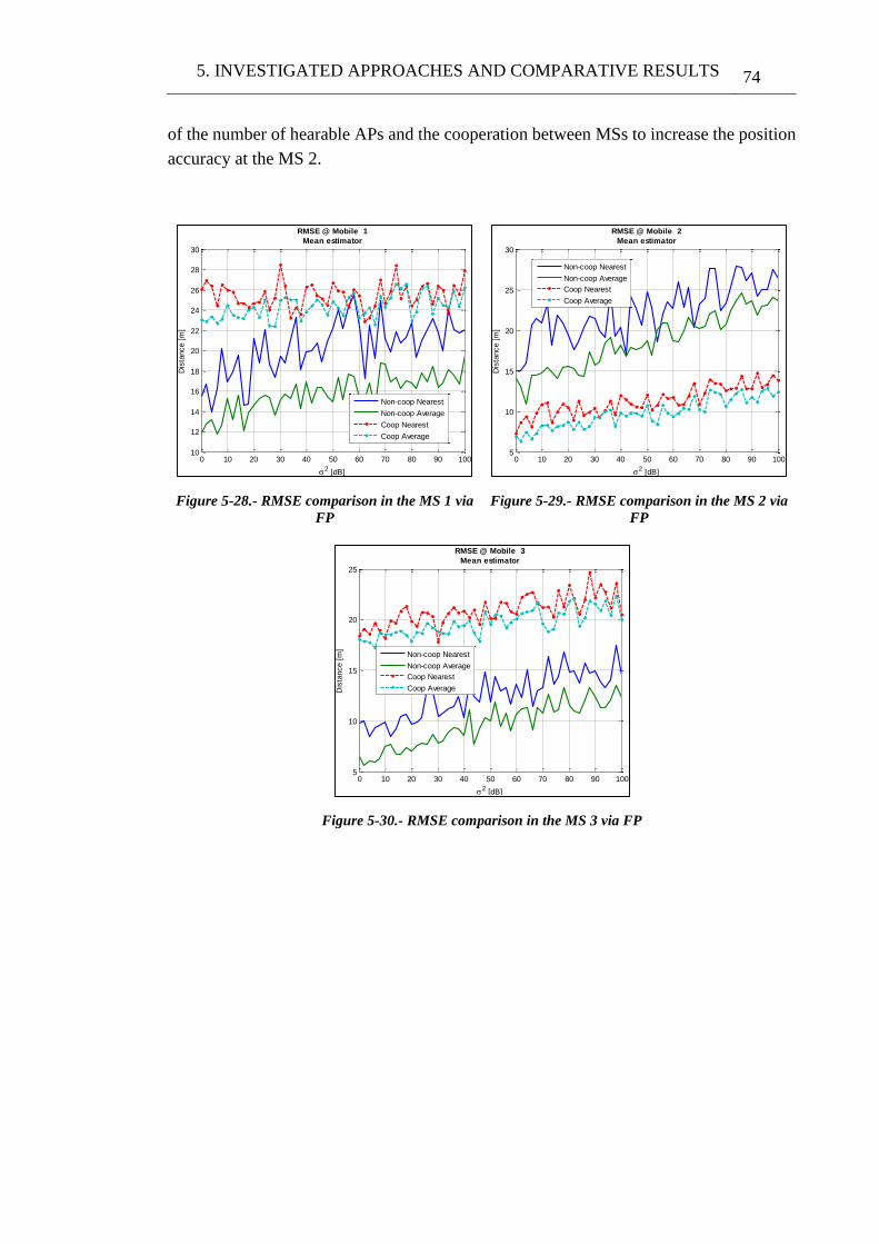
5. INVESTIGATED APPROACHES AND COMPARATIVE RESULTS 74
of the number of hearable APs and the cooperation between MSs to increase the position
accuracy at the MS 2.
Figure 5-28.- RMSE comparison in the MS 1 via
FP
Figure 5-29.- RMSE comparison in the MS 2 via
FP
Figure 5-30.- RMSE comparison in the MS 3 via FP
0 10 20 30 40 50 60 70 80 90 10010
12
14
16
18
20
22
24
26
28
30
2 [dB]
Dis
tance [
m]
RMSE @ Mobile 1
Mean estimator
Non-coop Nearest
Non-coop Average
Coop Nearest
Coop Average
0 10 20 30 40 50 60 70 80 90 1005
10
15
20
25
30
2 [dB]
Dis
tance [
m]
RMSE @ Mobile 2
Mean estimator
Non-coop Nearest
Non-coop Average
Coop Nearest
Coop Average
0 10 20 30 40 50 60 70 80 90 1005
10
15
20
25
2 [dB]
Dis
tance [
m]
RMSE @ Mobile 3
Mean estimator
Non-coop Nearest
Non-coop Average
Coop Nearest
Coop Average
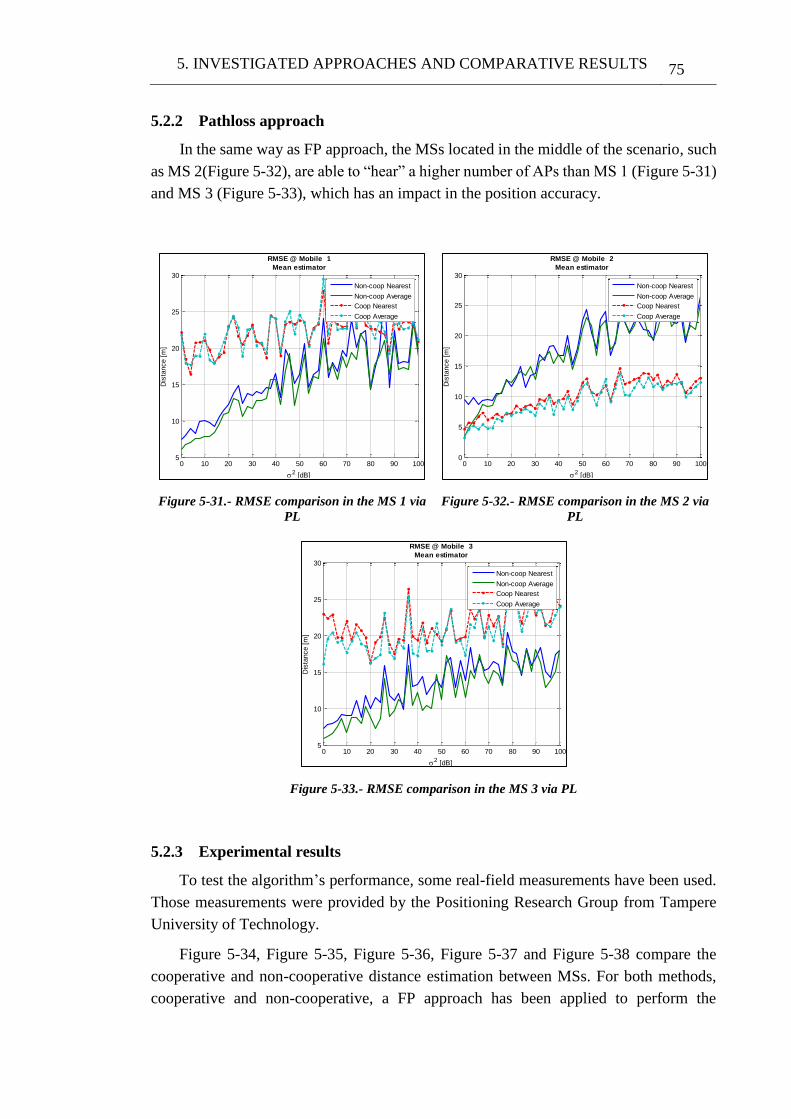
5. INVESTIGATED APPROACHES AND COMPARATIVE RESULTS 75
5.2.2 Pathloss approach
In the same way as FP approach, the MSs located in the middle of the scenario, such
as MS 2(Figure 5-32), are able to “hear” a higher number of APs than MS 1 (Figure 5-31)
and MS 3 (Figure 5-33), which has an impact in the position accuracy.
Figure 5-31.- RMSE comparison in the MS 1 via
PL
Figure 5-32.- RMSE comparison in the MS 2 via
PL
Figure 5-33.- RMSE comparison in the MS 3 via PL
5.2.3 Experimental results
To test the algorithm’s performance, some real-field measurements have been used.
Those measurements were provided by the Positioning Research Group from Tampere
University of Technology.
Figure 5-34, Figure 5-35, Figure 5-36, Figure 5-37 and Figure 5-38 compare the
cooperative and non-cooperative distance estimation between MSs. For both methods,
cooperative and non-cooperative, a FP approach has been applied to perform the
0 10 20 30 40 50 60 70 80 90 1005
10
15
20
25
30
2 [dB]
Dis
tance [
m]
RMSE @ Mobile 1
Mean estimator
Non-coop Nearest
Non-coop Average
Coop Nearest
Coop Average
0 10 20 30 40 50 60 70 80 90 1000
5
10
15
20
25
30
2 [dB]
Dis
tance [
m]
RMSE @ Mobile 2
Mean estimator
Non-coop Nearest
Non-coop Average
Coop Nearest
Coop Average
0 10 20 30 40 50 60 70 80 90 1005
10
15
20
25
30
2 [dB]
Dis
tance [
m]
RMSE @ Mobile 3
Mean estimator
Non-coop Nearest
Non-coop Average
Coop Nearest
Coop Average
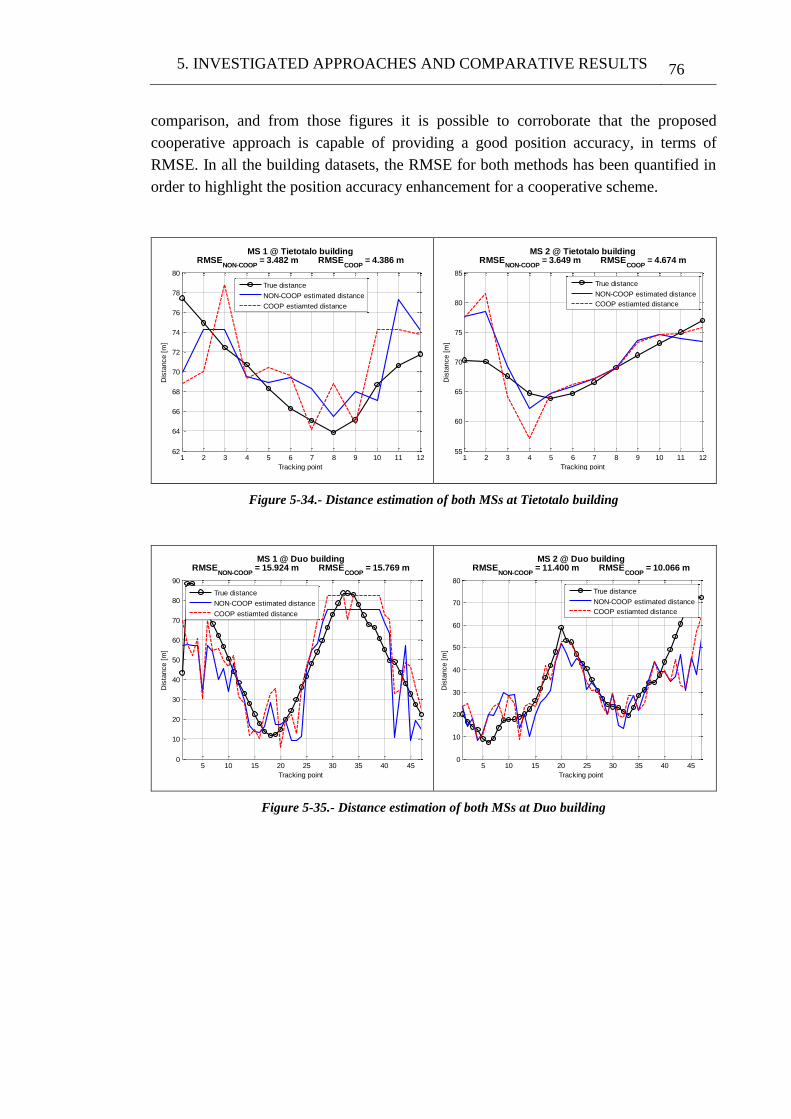
5. INVESTIGATED APPROACHES AND COMPARATIVE RESULTS 76
comparison, and from those figures it is possible to corroborate that the proposed
cooperative approach is capable of providing a good position accuracy, in terms of
RMSE. In all the building datasets, the RMSE for both methods has been quantified in
order to highlight the position accuracy enhancement for a cooperative scheme.
Figure 5-34.- Distance estimation of both MSs at Tietotalo building
Figure 5-35.- Distance estimation of both MSs at Duo building
1 2 3 4 5 6 7 8 9 10 11 1262
64
66
68
70
72
74
76
78
80
Tracking point
Dis
tance [
m]
MS 1 @ Tietotalo buildingRMSE
NON-COOP = 3.482 m RMSE
COOP = 4.386 m
True distance
NON-COOP estimated distance
COOP estiamted distance
1 2 3 4 5 6 7 8 9 10 11 1255
60
65
70
75
80
85
Tracking point
Dis
tance [
m]
MS 2 @ Tietotalo buildingRMSE
NON-COOP = 3.649 m RMSE
COOP = 4.674 m
True distance
NON-COOP estimated distance
COOP estiamted distance
5 10 15 20 25 30 35 40 450
10
20
30
40
50
60
70
80
90
Tracking point
Dis
tance [
m]
MS 1 @ Duo buildingRMSE
NON-COOP = 15.924 m RMSE
COOP = 15.769 m
True distance
NON-COOP estimated distance
COOP estiamted distance
5 10 15 20 25 30 35 40 450
10
20
30
40
50
60
70
80
Tracking point
Dis
tance [
m]
MS 2 @ Duo buildingRMSE
NON-COOP = 11.400 m RMSE
COOP = 10.066 m
True distance
NON-COOP estimated distance
COOP estiamted distance
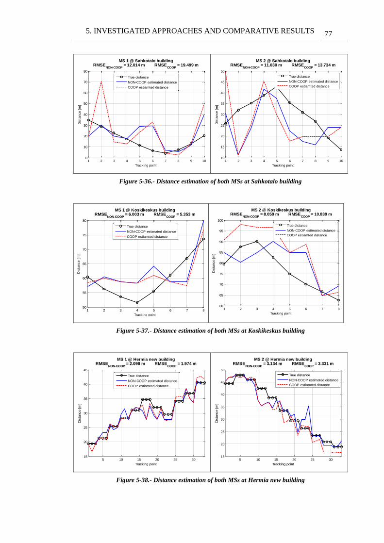
5. INVESTIGATED APPROACHES AND COMPARATIVE RESULTS 77
Figure 5-36.- Distance estimation of both MSs at Sahkotalo building
Figure 5-37.- Distance estimation of both MSs at Koskikeskus building
Figure 5-38.- Distance estimation of both MSs at Hermia new building
1 2 3 4 5 6 7 8 9 100
10
20
30
40
50
60
70
80
Tracking point
Dis
tance [
m]
MS 1 @ Sahkotalo buildingRMSE
NON-COOP = 12.014 m RMSE
COOP = 19.499 m
True distance
NON-COOP estimated distance
COOP estiamted distance
1 2 3 4 5 6 7 8 9 1010
15
20
25
30
35
40
45
50
Tracking point
Dis
tance [
m]
MS 2 @ Sahkotalo buildingRMSE
NON-COOP = 11.030 m RMSE
COOP = 13.734 m
True distance
NON-COOP estimated distance
COOP estiamted distance
1 2 3 4 5 6 7 850
55
60
65
70
75
80
Tracking point
Dis
tance [
m]
MS 1 @ Koskikeskus buildingRMSE
NON-COOP = 6.003 m RMSE
COOP = 5.353 m
True distance
NON-COOP estimated distance
COOP estiamted distance
1 2 3 4 5 6 7 860
65
70
75
80
85
90
95
100
Tracking point
Dis
tance [
m]
MS 2 @ Koskikeskus buildingRMSE
NON-COOP = 8.059 m RMSE
COOP = 10.839 m
True distance
NON-COOP estimated distance
COOP estiamted distance
5 10 15 20 25 3015
20
25
30
35
40
45
Tracking point
Dis
tance [
m]
MS 1 @ Hermia new buildingRMSE
NON-COOP = 2.098 m RMSE
COOP = 1.974 m
True distance
NON-COOP estimated distance
COOP estiamted distance
5 10 15 20 25 3015
20
25
30
35
40
45
50
Tracking point
Dis
tance [
m]
MS 2 @ Hermia new buildingRMSE
NON-COOP = 3.134 m RMSE
COOP = 3.331 m
True distance
NON-COOP estimated distance
COOP estiamted distance
6 Conclusions and open directions
In a broad sense, the aim of the thesis has been to study distance-based positioning
techniques for WLANs. We assumed the RSS simulation measurements with unknown
statistics from the network devices as information sources, and these measurements were
used in cooperative and non-cooperative algorithms to estimate the MS positions.
The thesis comprises several theoretical contributions from the current open
literature which were presented and described in Chapters 3 and 4, and amongst all of
them, we highlight the studies of cooperative networks. Specifically, the position
accuracy shown in Chapter 5 revealed important insights into the nature of “heard” AP’s
uncertainty and the effect of cooperation between MSs. Those factors have a great impact
in the position accuracy in terms of RMSE and they are dependent of the APs coverage
capability. Also, as shown in the results, FP and PL approaches have notorious
differences in terms of RMSE, and this is due to the implication of the shadowing during
the online phase, which increases the position accuracy. Thanks to the measured data
from real devices, it was possible to address the performance of both methods,
cooperative and non-cooperative. Each algorithm can be more or less useful depending
on the scenario in which applied. For example, in some buildings, such as: Duo,
Koskikeskus and Hermia, the RMSE can achieve a lower value.
Regarding the proposed cooperative approach, it has to be said that the algorithm is
robust, since it always provides reasonable results, even in very demanding conditions,
but its accuracy is very poor at the MSs located in the limits of the scenario, in
comparison with the non-cooperative approaches in a low density APs presence. Even
though the MSs located in the middle of the scenario can overcome this problem and
present an enhanced position accuracy substantially better than non-cooperative
approaches.
Indoor positioning in wireless networks is a very interesting field of research
nowadays, and many research efforts focus on it. The work done in this thesis is only a
small part of what can be done. An open issue is to use a more complex cost function in
the proposed cooperative approach in order to increase the position accuracy, also change
the Brute Force algorithm by Lagrange multiplier with the aim of providing a more
efficient software solution. Additionally, there are many unsolved challenges still in
indoor positioning, such as regarding hybridization of several localization sources,
security and privacy of the achieved solutions and complexity and battery consumption
of cooperative WLAN localization approaches.
7 References
[1] C. L. F. Mayorga, F. della Rosa, S. A. Wardana, G. Simone, M. C. N. Raynal, J.
Figueiras, and S. Frattasi, “Cooperative Positioning Techniques for Mobile
Localization in 4G Cellular Networks,” in International Conference on Pervasive
Services, 2007.
[2] F. Della Rosa, H. Leppäkoski, A. Ghalib, L. Ghazanfari, O. Garcia, S. Frattasi,
and J. Nurmi, “Ad Hoc Networks for Cooperative Mobile Positioning,” in in
Mobile Ad-Hoc Networks: Applications, X. Wang, Ed. Rijeka: InTech, 2011.
[3] Nokia, “Accurate Mobile Indoor Positioning Industry Alliance, called In-
Location, to promote deployment of location-based indoor services and
solutions,” Nokia - Press Release, 2012. [Online]. Available:
http://press.nokia.com/2012/08/23/accurate-mobile-indoor-positioning-industry-
alliance-called-in-location-to-promote-deployment-of-location-based-indoor-
services-and-solutions/. [Accessed: 02-Aug-2013].
[4] C. Yang, T. Nguyen, D. Venable, M. White, and R. Siegel, “Cooperative position
location with signals of opportunity,” in National Aerospace & Electronics
Conference, 2009.
[5] F. Della Rosa, S. A. Wardana, C. L. F. Mayorga, G. Simone, M. C. N. Raynal, J.
Figueiras, and S. Frattasi, “Experimental Activity on Cooperative Mobile
Positioning in Indoor Environments,” Int. Symp. a World Wireless, Mob.
Multimed. Networks, Jun. 2007.
[6] A. S. Soork, R. Saadat, and A. A. Tadaion, “Cooperative mobile positioning based
on Received Signal Strength,” Int. Symp. Telecommun., Aug. 2008.
[7] F. Della Rosa, L. Xu, J. Nurmi, C. Laoudias, M. Pelosi, and A. Terrezza, “Hand-
grip and body-loss impact on RSS measurements for localization of mass market
devices,” in International Conference on Localization and GNSS, 2011.
[8] A. Bel i Pereira, “A Pragmatic Approach of Localization and Tracking Algorithms
in Wireless Sensor Networks,” Universitat Autònoma de Barcelona, 2012.
[9] M. Gast, 802.11 Wireless Networks - The Definitive Guide. California: O’Reilly
Media, 2002.
[10] J. Schillerd, Mobile Communications, Second. Harlow: Pearson Education, 2003.
7. REFERENCES 80
[11] D. Tipper, “Lecture 1 - Cellular and Wireless Networks,” in in Cellular and
Wireless Networks, S. of Information Science, Ed. Pensilvania: University of
Pittsburgh, 2008.
[12] T. Ristaniemi, M. Renfors, and J. Niemelä, “Lecture 5 - Wireless Networks (802
family),” in in Basic Course on Wireless Communications, D. of Communications
Engineering, Ed. Tampere: Tampere Univeristy of Technology, 2011.
[13] A. Al-Fuqaha, “Lecture 14 - Wireless Personal Area Networks (WPANs),” in in
Wireless Networks, D. Computer Science, Ed. Michigan: Western Michigan
University, 2009.
[14] D. Singelée, F.-L. Wong, B. Preneel, and F. Stajano, “A Theoretical Model for
Location Privacy in Wireless Personal Area Networks.” Leuven, 2008.
[15] K. Pahlavan and P. Krishnamurthy, “Chapter 13 - Ad Hoc Networking and
WPAN,” in in Principles of Wireless Networks: A Unified Approach, New Jersey:
Prentice-Hall, 2002.
[16] D. Tipper, “Lecture 16 - Wireless Personal Area Networks,” in in Cellular and
Wireless Networks, vol. 15, S. of Information Science, Ed. Pensilvania: University
of Pittsburgh, 2008.
[17] S. Coleri Ergen, “ZigBee/IEEE 802.15.4 Summary.” California, 2004.
[18] H. Labiod, H. Afifi, and C. De Santis, Wi-Fi, Bluetooth, ZigBee and WiMax.
Dordrecht: Springer, 2007.
[19] S. Farahani, ZigBee Wireless Networks and Transceivers. Oxford: Elsevier, 2008.
[20] N. A. Somani and Y. Patel, “ZigBee: A Low Power Wireless Technology for
Industrial Applications,” Int. J. Control Theory Comput. Model., vol. 2, 2012.
[21] M. Ortuño, “Tema 2 - IEEE 802.11,” in in Redes Inalámbricas e Internet, D. de
Sistemas Telematicos y Computacion, Ed. Madrid: Univerdad Rey Juan Carlos,
2012.
[22] W.-F. Alliance, “Wi-Fi Certified.” [Online]. Available: https://www.wi-
fi.org/discover-and-learn. [Accessed: 24-Nov-2013].
[23] B. Sidhu, H. Singh, and A. Chhabra, “Emerging Wireless Standards - WiFi ,
ZigBee and WiMAX,” Int. J. Commun. Sci. Eng., 2007.
[24] M. T. Quer, “Designing a Frequency Selective Scheduler for WiMAX using
Genetic Algorithms,” University of Stuttgart, 2008.
[25] W. Forum, “WiMAX Forum.” [Online]. Available: http://www.wimaxforum.org/.
[Accessed: 30-Nov-2013].
7. REFERENCES 81
[26] A. Valdovinos, “Tema 7 - Redes WLAN y WMAN: Wi-Fi y WiMAX,” in in
Redes de Acceso Celular, D. de Ingeniería Electrónica y Comunicaciones, Ed.
Zaragoza: Universidad de Zaragoza, 2011.
[27] S. Andreev, “Energy Efficient and Cooperative Solutions for Next-Generation
Wireless Networks,” Tampere University of Technology, 2012.
[28] H. Liu, S. Member, H. Darabi, P. Banerjee, and J. Liu, “Survey of Wireless Indoor
Positioning Techniques and Systems,” Syst. Man, Cybern. Part C Appl. Rev.,
2007.
[29] K. Das, “Censoring for cooperative positioning,” Chalmers University of
Technology, 2010.
[30] T. Ristaniemi, M. Renfors, and J. Niemelä, “Lecture 2 - Radio channel
characteristics,” in in Basic Course on Wireless Communications, D. of
Communications Engineering, Ed. Tampere: Tampere Univeristy of Technology,
2011.
[31] G. Destino, “Positioning in Wireless Networks: Non-cooperative and cooperative
algorithms,” University of Oulu, 2012.
[32] A. A. Ali and A. S. Omar, “Time of Arrival Estimation for WLAN Indoor
Positioning Systems using Matrix Pencil Super Resolution Algorithm,” Work.
Positioning, Navig. Commun., 2005.
[33] W. Liu, H. Ding, X. Huang, X. Li, and J. Yuan, “Preliminary study on
noncooperative positioning using UWB impulse radio,” Int. Conf. Ultra-
Wideband, Sep. 2012.
[34] C. Yang, Y. Huang, and X. Zhu, “Hybrid TDOA/AOA Method for Indoor
Positioning,” Inst. Eng. Technol. Semin. Locat. Technol., 2007.
[35] M. Bocquet, C. Loyez, and A. Benlarbi-delaï, “Using Enhanced-TDOA
Measurement for Indoor Positioning,” Microw. Wirel. Components Lett., 2005.
[36] J. Kietlinski-zaleski, T. Yamazato, and M. Katayama, “TDOA UWB Positioning
With Three Receivers Using Known Indoor Features,” Int. Conf. Ultra-Wideband,
Sep. 2010.
[37] S. B. Wibowo, M. Klepal, and D. Pesch, “Time of Flight Ranging using Off-the-
self IEEE802 . 11 WiFi Tags,” Int. Conf. Position. Context., 2009.
[38] A. Günther and C. Hoene, “Measuring Round Trip Times to Determine the
Distance between WLAN Nodes,” Int. Proc. Netw., 2005.
[39] C. Wong, R. Klukas, and G. G. Messier, “Using WLAN Infrastructure for Angle-
of-Arrival Indoor User Location,” Veh. Technol. Conf., Sep. 2008.
7. REFERENCES 82
[40] X. Wang, A. K. Wong, and Y. Kong, “Mobility Tracking using GPS, Wi-Fi and
Cell ID,” Int. Conf. Inf. Netw., 2012.
[41] V. Honkavirta, T. Perälä, and R. Piché, “A Comparative Survey of WLAN
Location Fingerprinting Methods,” in Workshop on Positioning, Navigation and
Communication, 2009, vol. 2009, no. 1.
[42] F. Della Rosa, H. Leppäkoski, S. Biancullo, and J. Nurmi, “Ad hoc Networks
Aiding Indoor Calibrations of Heterogeneous Devices for Fingerprinting
Applications,” in International Conference on Indoor Positioning and Indoor
Navigation, 2010, no. September.
[43] H. Nurminen, J. Talvitie, S. Ali-löytty, P. Müller, E. Lohan, R. Piché, and M.
Renfors, “Statistical Path Loss Parameter Estimation and Positioning Using RSS
Measurements in Indoor Wireless Networks,” Int. Conf. Indoor Position. Indoor
Navig., no. November, 2012.
[44] F. Della Rosa, T. Paakki, H. Leppäkoski, and J. Nurmi, “A Cooperative
Framework for Path Loss Calibration and Indoor Mobile Positioning,” in
Workshop on Positioning, Navigation and Communication, 2010.
[45] S. Shrestha, J. Talvitie, and E. S. Lohan, “Deconvolution-based Indoor
Localization with WLAN Signals and Unknown Access Point Locations,” Int.
Conf. Localization GNSS, 2013.
[46] E. Laitinen, E. S. Lohan, J. Talvitie, and S. Shrestha, “Access point significance
measures in WLAN-based location,” Work. Positioning, Navig. Commun., Mar.
2012.
[47] J. Machaj, P. Brida, and R. Piché, “Rank Based Fingerprinting Algorithm for
Indoor Positioning,” Int. Conf. Indoor Position. Indoor Navig., Sep. 2011.
[48] C. Systems, “Lecture 4 - Indoor positioning using WLAN signals,” TKT-2546
Methods Position.
[49] F. Della Rosa, L. Xu, H. Leppäkoski, and J. Nurmi, “Relative Positioning of Mass
Market Devices in Ad hoc Networks,” in International Conference on Indoor
Positioning and Indoor Navigation, 2011.
[50] S.-H. Fang and T.-N. Lin, “Cooperative multi-radio localization in heterogeneous
wireless networks,” IEEE Trans. Wirel. Commun., May 2010.
[51] C. Mensing and J. J. Nielsen, “Centralized cooperative positioning and tracking
with realistic communications constraints,” Work. Positioning, Navig. Commun.,
Mar. 2010.
[52] H. Wymeersch, J. Lien, and M. Z. Win, “Cooperative Localization in Wireless
Networks,” Proc. IEEE, Feb. 2009.
7. REFERENCES 83
[53] S. Frattasi, “Link Layer Techniques Enabling Cooperation in 4G Wireless
Networks,” Aalborg Universitet, 2007.
[54] F. K. W. Chan and H. C. So, “Accurate Distributed Range-Based Positioning
Algorithm for Wireless Sensor Networks,” IEEE Trans. Signal Process., 2009.
[55] F. P. Rubio, “Cooperative localization algorithms in ultra-wideband systems for
indoor positioning,” Royal Institute of Technology, 2012.
[56] J. Nie, K. Ranestad, and B. Sturmfels, “The Algebraic Degree of Semidefinite
Programming,” Math. Program., Nov. 2008.
[57] K. Wing Kin Lui, W.-K. Ma, H. C. So, and F. Kit Wing Chan, “Semi-Definite
Programming Algorithms for Sensor Network Node Localization With
Uncertainties in Anchor Positions and/or Propagation Speed,” IEEE Trans. Signal
Process., 2009.
[58] P. Biswas, T. Liang, K. Toh, T. Wang, and Y. Ye, “Semidefinite Programming
Approaches for Sensor Network Localization with Noisy Distance
Measurements,” IEEE Trans. Autom. Sci. Eng., 2006.
[59] P. Biswas, T. Liang, T. Wang, and Y. Ye, “Semidefinite Programming Based
Algorithms for Sensor Network Localization,” ACM Trans. Sens. Networks, 2006.
[60] P. Biswas and Y. Ye, “Semidefinite Programming for Ad Hoc Wireless Sensor
Network Localization,” Int. Symp. Inf. Process. Sens. Networks, 2004.
[61] L. Wilkinson, “Multidimensional Scaling,” in in Desktop Data Analysis SYSTAT,
New Jersey: Prentice Hall, 1996, pp. 185–214.
[62] F. Wickelmaier, “An Introduction to MDS.” Aalborg, 2003.
[63] O.-H. Kwon and H.-J. Song, “Localization through Map Stitching in Wireless
Sensor Networks,” Trans. Parallel Distrib. Syst., 2008.
[64] J. A. Costa, N. Patwari, and A. O. H. Iii, “Distributed Weighted-Multidimensional
Scaling for Node Localization in Sensor Networks,” ACM Trans. Sens. Networks,
2005.
[65] M. Rahman, M. Z. Rahman, D. Habibi, and I. Ahmad, “Source Localisation in
Wireless Sensor Networks Based on Optimised Maximum Likelihood Source
Localisation in Wireless Sensor Networks Based on Optimised Maximum
Likelihood,” no. 2008.
[66] O. S. Oguejiofor, A. N. Aniedu, H. C. Ejiofor, and A. U. Okolibe, “Trilateration
Based localization Algorithm for Wireless Sensor Network,” Int. J. Sci. Mod.
Eng., 2013.
7. REFERENCES 84
[67] H. Avissar, “Non-parametric Belief Propagation Applications,” The Hebrew
University of Jerusalem, 2009.
[68] P. Christensson, “Ad Hoc Network,” Tech Terms Computer Dictionary, 2006.
[Online]. Available: http://www.techterms.com/definition/adhocnetwork.
[Accessed: 04-Aug-2013].
[69] T. Mickelsson, “ATM versus Ethernet,” 1999. [Online]. Available:
http://www.tml.tkk.fi/Opinnot/Tik-
110.551/1999/papers/07ATMvsEthernet/iworkpaper.html. [Accessed: 01-Dec-
2013].
[70] P. Christensson, “P2P,” Tech Terms Computer Dictionary, 2006. [Online].
Available: http://www.techterms.com/definition/p2p. [Accessed: 04-Dec-2013].
[71] J. Míguez, D. Crisan, and P. M. Djuric, “On the convergence of two sequential
Monte Carlo methods for maximum a posteriori sequence estimation and
stochastic global optimization,” Stat. Comput., 2011.
[72] F. James, “Monte Carlo theory and practice,” Reports Prog. Phys., 1980.
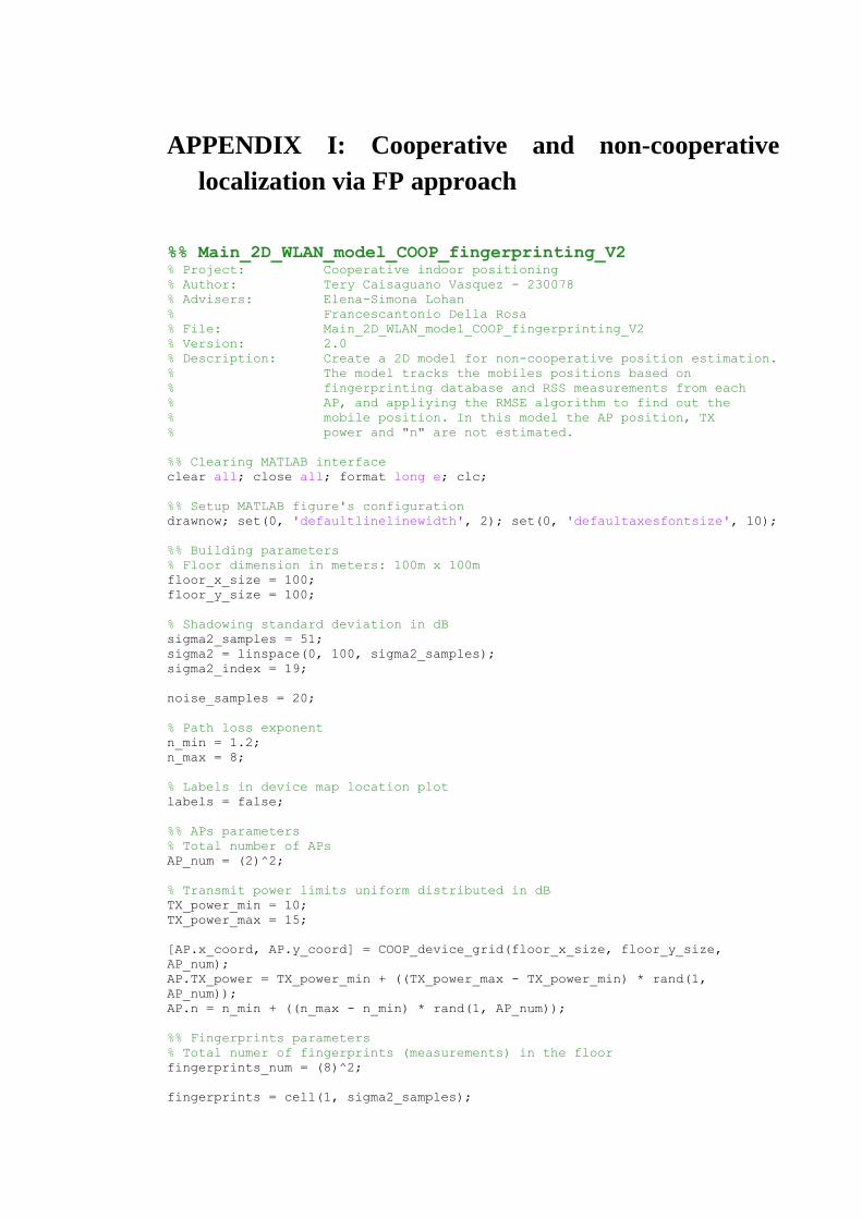
APPENDIX I: Cooperative and non-cooperative
localization via FP approach
%% Main_2D_WLAN_model_COOP_fingerprinting_V2 % Project: Cooperative indoor positioning
% Author: Tery Caisaguano Vasquez - 230078
% Advisers: Elena-Simona Lohan
% Francescantonio Della Rosa
% File: Main_2D_WLAN_model_COOP_fingerprinting_V2
% Version: 2.0
% Description: Create a 2D model for non-cooperative position estimation.
% The model tracks the mobiles positions based on
% fingerprinting database and RSS measurements from each
% AP, and appliying the RMSE algorithm to find out the
% mobile position. In this model the AP position, TX
% power and "n" are not estimated.
%% Clearing MATLAB interface
clear all; close all; format long e; clc;
%% Setup MATLAB figure's configuration
drawnow; set(0, 'defaultlinelinewidth', 2); set(0, 'defaultaxesfontsize', 10);
%% Building parameters
% Floor dimension in meters: 100m x 100m
floor_x_size = 100;
floor_y_size = 100;
% Shadowing standard deviation in dB
sigma2_samples = 51;
sigma2 = linspace(0, 100, sigma2_samples);
sigma2_index = 19;
noise_samples = 20;
% Path loss exponent
n_min = 1.2;
n_max = 8;
% Labels in device map location plot
labels = false;
%% APs parameters
% Total number of APs
AP_num = (2)^2;
% Transmit power limits uniform distributed in dB
TX_power_min = 10;
TX_power_max = 15;
[AP.x_coord, AP.y_coord] = COOP_device_grid(floor_x_size, floor_y_size,
AP_num);
AP.TX_power = TX_power_min + ((TX_power_max - TX_power_min) * rand(1,
AP_num));
AP.n = n_min + ((n_max - n_min) * rand(1, AP_num));
%% Fingerprints parameters
% Total numer of fingerprints (measurements) in the floor
fingerprints_num = (8)^2;
fingerprints = cell(1, sigma2_samples);
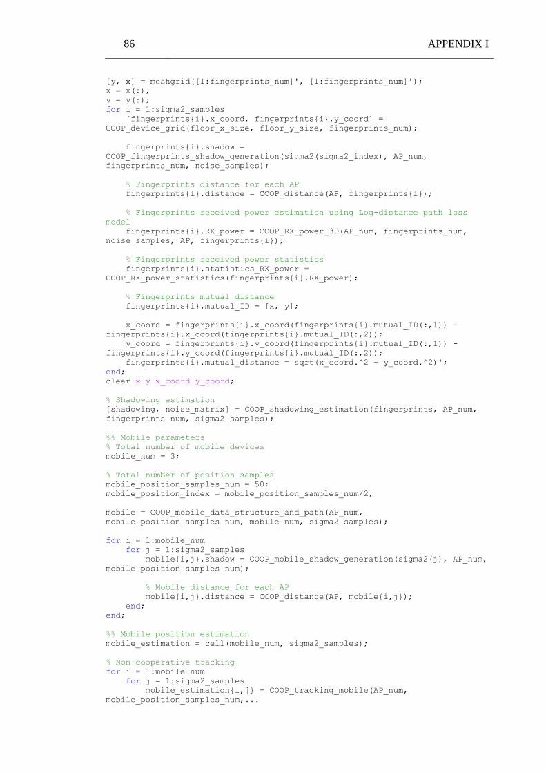
86 APPENDIX I
[y, x] = meshgrid([1:fingerprints_num]', [1:fingerprints_num]');
x = x(:);
y = y(:);
for i = 1:sigma2_samples
[fingerprints{i}.x_coord, fingerprints{i}.y_coord] =
COOP_device_grid(floor_x_size, floor_y_size, fingerprints_num);
fingerprints{i}.shadow =
COOP_fingerprints_shadow_generation(sigma2(sigma2_index), AP_num,
fingerprints_num, noise_samples);
% Fingerprints distance for each AP
fingerprints{i}.distance = COOP_distance(AP, fingerprints{i});
% Fingerprints received power estimation using Log-distance path loss
model
fingerprints{i}.RX_power = COOP_RX_power_3D(AP_num, fingerprints_num,
noise_samples, AP, fingerprints{i});
% Fingerprints received power statistics
fingerprints{i}.statistics_RX_power =
COOP_RX_power_statistics(fingerprints{i}.RX_power);
% Fingerprints mutual distance
fingerprints{i}.mutual_ID = [x, y];
x_coord = fingerprints{i}.x_coord(fingerprints{i}.mutual_ID(:,1)) -
fingerprints{i}.x_coord(fingerprints{i}.mutual_ID(:,2));
y_coord = fingerprints{i}.y_coord(fingerprints{i}.mutual_ID(:,1)) -
fingerprints{i}.y_coord(fingerprints{i}.mutual_ID(:,2));
fingerprints{i}.mutual_distance = sqrt(x_coord.^2 + y_coord.^2)';
end;
clear x y x_coord y_coord;
% Shadowing estimation
[shadowing, noise_matrix] = COOP_shadowing_estimation(fingerprints, AP_num,
fingerprints_num, sigma2_samples);
%% Mobile parameters
% Total number of mobile devices
mobile_num = 3;
% Total number of position samples
mobile_position_samples_num = 50;
mobile_position_index = mobile_position_samples_num/2;
mobile = COOP_mobile_data_structure_and_path(AP_num,
mobile_position_samples_num, mobile_num, sigma2_samples);
for i = 1:mobile_num
for j = 1:sigma2_samples
mobile{i,j}.shadow = COOP_mobile_shadow_generation(sigma2(j), AP_num,
mobile_position_samples_num);
% Mobile distance for each AP
mobile{i,j}.distance = COOP_distance(AP, mobile{i,j});
end;
end;
%% Mobile position estimation
mobile_estimation = cell(mobile_num, sigma2_samples);
% Non-cooperative tracking
for i = 1:mobile_num
for j = 1:sigma2_samples
mobile_estimation{i,j} = COOP_tracking_mobile(AP_num,
mobile_position_samples_num,...
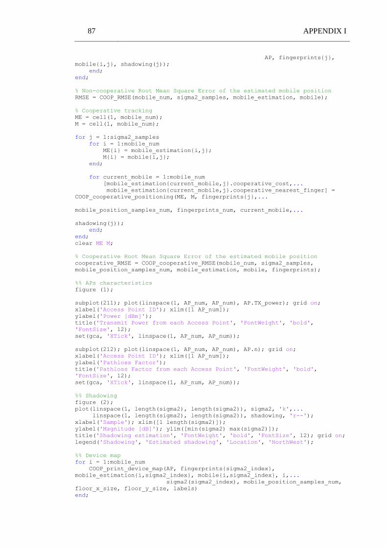
87 APPENDIX I
AP, fingerprints{j},
mobile{i,j}, shadowing(j));
end;
end;
% Non-cooperative Root Mean Square Error of the estimated mobile position
RMSE = COOP_RMSE(mobile_num, sigma2_samples, mobile_estimation, mobile);
% Cooperative tracking
ME = cell(1, mobile_num);
M = cell(1, mobile_num);
for j = 1:sigma2_samples
for i = 1:mobile_num
ME{i} = mobile_estimation{i,j};
M{i} = mobile{i,j};
end;
for current_mobile = 1:mobile_num
[mobile_estimation{current_mobile,j}.cooperative_cost,...
mobile_estimation{current_mobile,j}.cooperative_nearest_finger] =
COOP_cooperative_positioning(ME, M, fingerprints{j},...
mobile_position_samples_num, fingerprints_num, current_mobile,...
shadowing(j));
end;
end;
clear ME M;
% Cooperative Root Mean Square Error of the estimated mobile position
cooperative_RMSE = COOP_cooperative_RMSE(mobile_num, sigma2_samples,
mobile_position_samples_num, mobile_estimation, mobile, fingerprints);
%% APs characteristics
figure (1);
subplot(211); plot(linspace(1, AP_num, AP_num), AP.TX_power); grid on;
xlabel('Access Point ID'); xlim([1 AP_num]);
ylabel('Power [dBm]');
title('Transmit Power from each Access Point', 'FontWeight', 'bold',
'FontSize', 12);
set(gca, 'XTick', linspace(1, AP_num, AP_num));
subplot(212); plot(linspace(1, AP_num, AP_num), AP.n); grid on;
xlabel('Access Point ID'); xlim([1 AP_num]);
ylabel('Pathloss Factor');
title('Pathloss Factor from each Access Point', 'FontWeight', 'bold',
'FontSize', 12);
set(gca, 'XTick', linspace(1, AP_num, AP_num));
%% Shadowing
figure (2);
plot(linspace(1, length(sigma2), length(sigma2)), sigma2, 'k',...
linspace(1, length(sigma2), length(sigma2)), shadowing, 'r--');
xlabel('Sample'); xlim([1 length(sigma2)]);
ylabel('Magnitude [dB]'); ylim([min(sigma2) max(sigma2)]);
title('Shadowing estimation', 'FontWeight', 'bold', 'FontSize', 12); grid on;
legend('Shadowing', 'Estimated shadowing', 'Location', 'NorthWest');
%% Device map
for i = 1:mobile_num
COOP_print_device_map(AP, fingerprints{sigma2_index},
mobile_estimation{i,sigma2_index}, mobile{i,sigma2_index}, i,...
sigma2(sigma2_index), mobile_position_samples_num,
floor_x_size, floor_y_size, labels)
end;
88 APPENDIX I
%% Non-cooperative RMSE for each mobile estimation
for i = 1:mobile_num
figure (5 + i);
subplot(211);
plot(sigma2, RMSE.nearest_neighbor.mean(i,:),...
sigma2, RMSE.nearest_neighbor.median(i,:),...
sigma2, RMSE.nearest_neighbor.max(i,:),...
sigma2, RMSE.nearest_neighbor.mode(i,:));
set(gca, 'YTick',
[floor(min(RMSE.nearest_neighbor.max(i,:))):8:ceil(max(RMSE.nearest_neighbor.m
ax(i,:)))]); grid on;
xlabel('\sigma^2 [dB]'); xlim([min(sigma2) max(sigma2)]);
ylabel('Distance [m]'); ylim([0 max(RMSE.nearest_neighbor.max(i,:))]);
buffer_text = sprintf('Non-cooperative RMSE Nearest Neighbor @ Mobile
%2d', i);
title(buffer_text, 'FontWeight', 'bold', 'FontSize', 10);
legend('Mean', 'Median', 'Max', 'Most recurrent', 'Location',
'EastOutside');
subplot(212);
plot(sigma2, RMSE.average.mean(i,:),...
sigma2, RMSE.average.median(i,:),...
sigma2, RMSE.average.max(i,:),...
sigma2, RMSE.average.mode(i,:));
set(gca, 'YTick',
[floor(min(RMSE.average.max(i,:))):8:ceil(max(RMSE.average.max(i,:)))]); grid
on;
xlabel('\sigma^2 [dB]'); xlim([min(sigma2) max(sigma2)]);
ylabel('Distance [m]'); ylim([0 max(RMSE.average.max(i,:))]);
buffer_text = sprintf('Non-cooperative RMSE Average of Neighbors @ Mobile
%2d', i);
title(buffer_text, 'FontWeight', 'bold', 'FontSize', 10);
legend('Mean', 'Median', 'Max', 'Most recurrent', 'Location',
'EastOutside');
end;
%% Power maps for each AP
COOP_print_power_maps(AP, fingerprints{sigma2_index}, AP_num,
sigma2(sigma2_index));
%% Non-cooperative and Cooperative RMSE comparison
for i = 1:mobile_num
figure (15 + i);
plot(sigma2, RMSE.nearest_neighbor.mean(i,:),'-',...
sigma2, RMSE.average.mean(i,:),'-',...
sigma2, cooperative_RMSE.nearest_neighbor.mean(i,:),'.--',...
sigma2, cooperative_RMSE.average.mean(i,:),'.--');
xlabel('\sigma^2 [dB]'); xlim([min(sigma2) max(sigma2)]);
ylabel('Distance [m]');
buffer_text_line1 = sprintf('RMSE @ Mobile %2d', i);
buffer_text_line2 = sprintf('Mean estimator');
title({[buffer_text_line1], [buffer_text_line2]}, 'FontWeight', 'bold',
'FontSize', 10);
legend('Non-coop Nearest', 'Non-coop Average', 'Coop Nearest', 'Coop
Average', 'Location', 'Best'); grid on;
end;
89 APPENDIX I
function shadow = COOP_fingerprints_shadow_generation(sigma2, TX_num,
RX_num, noise_samples)
shadow = zeros(TX_num, RX_num, noise_samples);
for i = 1:noise_samples
for j = 1:RX_num
shadow(:,j,i) = randn(1, TX_num);
shadow(:,j,i) = sqrt(sigma2) * (shadow(:,j,i) -
mean(shadow(:,j,i))) / std(shadow(:,j,i));
end;
end;
end
function RX_power = COOP_RX_power_3D(TX_num, RX_num, noise_samples,
TX_device, RX_device)
%% Received power estimation using Log-distance path loss model
RX_power = zeros(TX_num, RX_num, noise_samples);
for i = 1:TX_num
for j = 1:RX_num
for k = 1:noise_samples
RX_power(i,j,k) = TX_device.TX_power(i) - (10 * TX_device.n(i)
* log10(RX_device.distance(i,j))) + RX_device.shadow(i,j,k);
end;
end;
end;
end
function [shadowing, noise_matrix] =
COOP_shadowing_estimation(fingerprints, AP_num, fingerprints_num,
sigma2_samples)
shadowing = zeros(1, sigma2_samples);
noise_matrix = zeros(AP_num, fingerprints_num, sigma2_samples);
for sigma2 = 1:sigma2_samples
noise_matrix(:,:,sigma2) = std(fingerprints{sigma2}.RX_power, 0, 3);
shadowing(sigma2) = (mean(mean(noise_matrix(:,:,sigma2), 2)))^2;
end;
end
function shadow = COOP_mobile_shadow_generation(sigma2, TX_num,
RX_num)
shadow = zeros(TX_num, RX_num);
for i = 1:RX_num
shadow(:,i) = randn(1, TX_num);
shadow(:,i) = sqrt(sigma2) * (shadow(:,i) - mean(shadow(:,i))) /
std(shadow(:,i));
end;
end
90 APPENDIX I
function mobile_estimation = COOP_tracking_mobile(AP_num,
mobile_position_samples_num,...
AP, fingerprints,
mobile, shadowing)
% Mobile received power estimation for each AP
mobile_estimation.RX_power = COOP_RX_power_2D(AP_num,
mobile_position_samples_num, AP, mobile);
% Average of 4 nearest neighbor
[mobile_estimation.avg_x_coord.mean,...
mobile_estimation.avg_y_coord.mean,...
mobile_estimation.MSE_mobile.mean,...
mobile_estimation.nearest_finger.mean] = COOP_position
(mobile_estimation.RX_power,...
fingerprints.statistics_RX_power.mean,...
fingerprints.x_coord,...
fingerprints.y_coord,...
shadowing);
[mobile_estimation.avg_x_coord.median,...
mobile_estimation.avg_y_coord.median,...
mobile_estimation.MSE_mobile.median,...
mobile_estimation.nearest_finger.median] = COOP_position
(mobile_estimation.RX_power,...
fingerprints.statistics_RX_power.median,...
fingerprints.x_coord,...
fingerprints.y_coord,...
shadowing);
[mobile_estimation.avg_x_coord.max,...
mobile_estimation.avg_y_coord.max,...
mobile_estimation.MSE_mobile.max,...
mobile_estimation.nearest_finger.max] = COOP_position
(mobile_estimation.RX_power,...
fingerprints.statistics_RX_power.max,...
fingerprints.x_coord,...
fingerprints.y_coord,...
shadowing);
[mobile_estimation.avg_x_coord.mode,...
mobile_estimation.avg_y_coord.mode,...
mobile_estimation.MSE_mobile.mode,...
mobile_estimation.nearest_finger.mode] = COOP_position
(mobile_estimation.RX_power,...
fingerprints.statistics_RX_power.mode,...
fingerprints.x_coord,...
fingerprints.y_coord,...
shadowing);
% Nearest Neighbor
mobile_estimation.nearest_x_coord.mean =
fingerprints.x_coord(mobile_estimation.nearest_finger.mean(:,1)');
91 APPENDIX I
mobile_estimation.nearest_y_coord.mean =
fingerprints.y_coord(mobile_estimation.nearest_finger.mean(:,1)');
mobile_estimation.nearest_x_coord.median =
fingerprints.x_coord(mobile_estimation.nearest_finger.median(:,1)');
mobile_estimation.nearest_y_coord.median =
fingerprints.y_coord(mobile_estimation.nearest_finger.median(:,1)');
mobile_estimation.nearest_x_coord.max =
fingerprints.x_coord(mobile_estimation.nearest_finger.max(:,1)');
mobile_estimation.nearest_y_coord.max =
fingerprints.y_coord(mobile_estimation.nearest_finger.max(:,1)');
mobile_estimation.nearest_x_coord.mode =
fingerprints.x_coord(mobile_estimation.nearest_finger.mode(:,1)');
mobile_estimation.nearest_y_coord.mode =
fingerprints.y_coord(mobile_estimation.nearest_finger.mode(:,1)');
end
function [mobile_RX_power, threshold_mobile, total_heared_APs] =
COOP_remove_low_powered_AP_signals(mobile_RX_power)
%% Initializing variables
total_heared_APs = zeros(1, size(mobile_RX_power, 1));
%% Defining received power thresholds
threshold_mobile = mean(mobile_RX_power, 1);
%% Removing low powered measurements
for i = 1:length(threshold_mobile)
removed_APs = mobile_RX_power(:, i) < threshold_mobile(i);
mobile_RX_power(removed_APs, i) = NaN;
total_heared_APs(i) = length(find(removed_APs == 0));
end;
end
function [avg_x_coord,...
avg_y_coord,...
MSE_mobile,...
nearest_finger] = COOP_position (mobile_RX_power,...
fingerprints_RX_power,...
fingerprints_x_coord,...
fingerprints_y_coord,...
shadowing)
%% Removing low powered singals
[mobile_RX_power, ~, total_heared_APs] =
COOP_remove_low_powered_AP_signals(mobile_RX_power);
%% Defining number of elements
AP_num = size(mobile_RX_power, 1);
mobile_position_samples_num = size(mobile_RX_power, 2);
fingerprints_num = size(fingerprints_RX_power, 2);
%% Nearest fingerprint estimation
p = 2;
cost = zeros(mobile_position_samples_num, AP_num, fingerprints_num);
for i = 1:mobile_position_samples_num
for j = 1:AP_num
92 APPENDIX I
if (isnan(mobile_RX_power(j,i)) == 0)
for k = 1:fingerprints_num
if (shadowing < 0.5)
cost(i,j,k) = (mobile_RX_power(j,i) -
fingerprints_RX_power(j,k))^p;
else
cost(i,j,k) = (1 / (sqrt(2 * pi * shadowing^2))) *
exp(-(mobile_RX_power(j,i) - fingerprints_RX_power(j,k))^p / (2 *
shadowing^2));
end;
end;
end;
end;
end;
MSE_mobile = zeros(mobile_position_samples_num, fingerprints_num);
for i = 1:mobile_position_samples_num
MSE_mobile(i,:) = (sum(cost(i,:,:))).^(1/p) / total_heared_APs(i);
end;
if (shadowing < 0.5)
[~, index_mse] = sort(MSE_mobile, 2, 'ascend');
else
[~, index_mse] = sort(MSE_mobile, 2, 'descend');
end;
%% Nearest Neighbor
nearest_finger = index_mse;
%% Average of 4 Nearest Neighbor
avg_x_coord = zeros(1, mobile_position_samples_num);
avg_y_coord = zeros(1, mobile_position_samples_num);
for i = 1:mobile_position_samples_num
avg_x_coord(i) = sum(fingerprints_x_coord(index_mse(i,1:4))) /
length(index_mse(i,1:4));
avg_y_coord(i) = sum(fingerprints_y_coord(index_mse(i,1:4))) /
length(index_mse(i,1:4));
end;
end
function [cooperative_cost, cooperative_nearest_finger] =
COOP_cooperative_positioning(mobile_estimation, mobile,
fingerprints,...
mobile_position_samples_num, fingerprints_num, current_mobile,...
shadowing)
%% Defining data structure
cooperative = struct('mean', [],...
'median', [],...
'max', [],...
'mode', []);
cooperative_cost = cooperative;
cooperative_cost.mean = cell(1,
length(mobile{current_mobile}.mobile_pairs));
cooperative_nearest_finger = cooperative;
cooperative_nearest_finger.mean = cell(1,
length(mobile{current_mobile}.mobile_pairs));
%% Cooperative cost function to be maximized
93 APPENDIX I
distance_difference = zeros(fingerprints_num^2,
mobile_position_samples_num);
cost = zeros(fingerprints_num^2, mobile_position_samples_num);
for m = 1:length(mobile{current_mobile}.mobile_pairs)
% Joint cost function
joint_cost = mobile_estimation{current_mobile}.MSE_mobile.mean' +
mobile_estimation{mobile{current_mobile}.mobile_pairs(m)}.MSE_mobile.mean';
% Distance difference criteria
for p = 1:mobile_position_samples_num
distance_difference(:,p) = sqrt(abs(fingerprints.mutual_distance -
(ones(fingerprints_num^2,1) * mobile{current_mobile}.mutual_distance(m,p))));
end;
% Cooperative cost function
for fp = 1:fingerprints_num
cost((((fp - 1) * fingerprints_num) + 1:fingerprints_num * fp),:)
= joint_cost - distance_difference((((fp - 1) * fingerprints_num) +
1:fingerprints_num * fp),:);
end;
% Maximization of the cooperative function
cooperative_nearest_finger.mean{m} =
zeros(fingerprints_num^2,mobile_position_samples_num,2);
for p = 1:mobile_position_samples_num
if (shadowing < 0.5)
[sorted_cost, index_cost] = sort(cost(:,p), 'ascend');
else
[sorted_cost, index_cost] = sort(cost(:,p), 'descend');
end
cooperative_cost.mean{m}(:,p) = sorted_cost;
cooperative_nearest_finger.mean{m}(:,p,1) =
fingerprints.mutual_ID(index_cost,1);
cooperative_nearest_finger.mean{m}(:,p,2) =
fingerprints.mutual_ID(index_cost,2);
end;
end;
end
APPENDIX II: Cooperative and non-cooperative
localization via PL approach
%% Main_2D_WLAN_model_COOP_path_loss_and_AP_estimation_V2 % Project: Cooperative indoor positioning
% Author: Tery Caisaguano Vasquez - 230078
% Advisers: Elena-Simona Lohan
% Francescantonio Della Rosa
% File: Main_2D_WLAN_model_COOP_path_loss_and_AP_estimation_V2
% Version: 2.0
% Description: Create a 2D model for non-cooperative position estimation.
% The model tracks the mobiles positions based on
% fingerprinting database and RSS measurements from each
% AP. Path Loss modelling is implemented to apply the ML
% algorithm to find out the mobile position. Also, the
% model estimates the AP position, TX power, shadowing
% standard deviation and "n" using the LS algoritm. Those
% estimated parameters are used for the mobile tracking.
%% Clearing MATLAB interface
clear all; close all; format long e; clc;
%% Setup MATLAB figure's configuration
drawnow; set(0, 'defaultlinelinewidth', 2); set(0, 'defaultaxesfontsize', 10);
%% Building parameters
% Floor dimension in meters: 100m x 100m
floor_x_size = 100;
floor_y_size = 100;
% Shadowing standard deviation in dB
sigma2_samples = 51;
sigma2 = linspace(0, 100, sigma2_samples);
sigma2_index = 19;
noise_samples = 20;
% Path loss exponent
n_min = 1.2;
n_max = 8;
% Labels in device map location plot
labels = false;
%% APs parameters
% Total number of APs
AP_num = (2)^2;
% Transmit power limits uniform distributed in dB
TX_power_min = 10;
TX_power_max = 15;
[AP.x_coord, AP.y_coord] = COOP_device_grid(floor_x_size, floor_y_size,
AP_num);
AP.TX_power = TX_power_min + ((TX_power_max - TX_power_min) * rand(1,
AP_num));
AP.n = n_min + ((n_max - n_min) * rand(1, AP_num));
%% Fingerprints parameters
% Total numer of fingerprints (measurements) in the floor
fingerprints_num = (8)^2;
95 APPENDIX II
fingerprints = cell(1, sigma2_samples);
[y, x] = meshgrid([1:fingerprints_num]', [1:fingerprints_num]');
x = x(:);
y = y(:);
for i = 1:sigma2_samples
[fingerprints{i}.x_coord, fingerprints{i}.y_coord] =
COOP_device_grid(floor_x_size, floor_y_size, fingerprints_num);
fingerprints{i}.shadow =
COOP_fingerprints_shadow_generation(sigma2(sigma2_index), AP_num,
fingerprints_num, noise_samples);
% Fingerprints distance for each AP
fingerprints{i}.distance = COOP_distance(AP, fingerprints{i});
% Fingerprints received power estimation using Log-distance path loss
model
fingerprints{i}.RX_power = COOP_RX_power_3D(AP_num, fingerprints_num,
noise_samples, AP, fingerprints{i});
% Fingerprints received power statistics
fingerprints{i}.statistics_RX_power =
COOP_RX_power_statistics(fingerprints{i}.RX_power);
% Fingerprints mutual distance
fingerprints{i}.mutual_ID = [x, y];
x_coord = fingerprints{i}.x_coord(fingerprints{i}.mutual_ID(:,1)) -
fingerprints{i}.x_coord(fingerprints{i}.mutual_ID(:,2));
y_coord = fingerprints{i}.y_coord(fingerprints{i}.mutual_ID(:,1)) -
fingerprints{i}.y_coord(fingerprints{i}.mutual_ID(:,2));
fingerprints{i}.mutual_distance = sqrt(x_coord.^2 + y_coord.^2)';
end;
clear x y x_coord y_coord;
% Shadowing estimation
[shadowing, noise_matrix] = COOP_shadowing_estimation(fingerprints, AP_num,
fingerprints_num, sigma2_samples);
%% APs parameteres estimation
AP_estimation = cell(1, sigma2_samples);
for i = 1:sigma2_samples
% Strongest fingerprint criterion
[AP_estimation{i}.x_coord, AP_estimation{i}.y_coord,
AP_estimation{i}.distance] = COOP_strongest_fingerprint(fingerprints{i},...
fingerprints_num,...
AP_num,...
floor_x_size,...
floor_y_size);
% Transmit power and path loss coefficient estimation
[AP_estimation{i}.TX_power, AP_estimation{i}.n] =
COOP_TX_power_and_path_loss_estimation(fingerprints{i},...
AP_estimation{i},...
noise_matrix(:,:,i),...
fingerprints_num,...
AP_num);
end;
96 APPENDIX II
%% Mobile parameters
% Total number of mobile devices
mobile_num = 3;
% Total number of position samples
mobile_position_samples_num = 50;
mobile_position_index = mobile_position_samples_num/2;
mobile = COOP_data_structure_and_mobiles_path(AP_num,
mobile_position_samples_num, mobile_num, sigma2_samples);
for i = 1:mobile_num
for j = 1:sigma2_samples
mobile{i,j}.shadow = COOP_mobile_shadow_generation(sigma2(j), AP_num,
mobile_position_samples_num);
% Mobile distance for each AP
mobile{i,j}.distance = COOP_distance_data_structure(AP_estimation{j},
mobile{i,j});
end;
end;
%% Mobile position estimation
mobile_estimation = cell(mobile_num, sigma2_samples);
% Non-cooperative tracking
for i = 1:mobile_num
for j = 1:sigma2_samples
mobile_estimation{i,j} = COOP_tracking_mobile(AP_num,
mobile_position_samples_num,...
AP_estimation{j},
fingerprints{j}, mobile{i,j}, shadowing(j));
end;
end;
% Non-cooperative Root Mean Square Error of the estimated mobile position
RMSE = COOP_RMSE(mobile_num, sigma2_samples, mobile_estimation, mobile);
% Cooperative tracking
ME = cell(1, mobile_num);
M = cell(1, mobile_num);
for j = 1:sigma2_samples
for i = 1:mobile_num
ME{i} = mobile_estimation{i,j};
M{i} = mobile{i,j};
end;
for current_mobile = 1:mobile_num
[mobile_estimation{current_mobile,j}.cooperative_cost,...
mobile_estimation{current_mobile,j}.cooperative_nearest_finger] =
COOP_cooperative_positioning(ME, M, fingerprints{j},...
mobile_position_samples_num, fingerprints_num, current_mobile);
end;
end;
% Cooperative Root Mean Square Error of the estimated mobile position
cooperative_RMSE = COOP_cooperative_RMSE(mobile_num, sigma2_samples,
mobile_position_samples_num, mobile_estimation, mobile, fingerprints);
%% APs characteristics
AP_ID = linspace(1, AP_num, AP_num);
figure (1);
97 APPENDIX II
subplot(211);
plot(AP_ID, AP_estimation{sigma2_index}.TX_power.mean, '--',...
AP_ID, AP_estimation{sigma2_index}.TX_power.median, '--',...
AP_ID, AP_estimation{sigma2_index}.TX_power.max, '--',...
AP_ID, AP_estimation{sigma2_index}.TX_power.mode, '--',...
AP_ID, AP.TX_power);
xlabel('Access Point ID'); xlim([1 AP_num]);
ylabel('Power [dBm]');
buffer_text_line1 = sprintf('Transmit Power for each Access Point');
buffer_text_line2 = sprintf('\\sigma^2 = %1.2f dB', sigma2(sigma2_index));
title({[buffer_text_line1], [buffer_text_line2]}, 'FontWeight', 'bold',
'FontSize', 10);
set(gca, 'XTick', AP_ID); grid on;
legend('Mean', 'Median', 'Max', 'Most recurrent', 'Transmitted Power',
'Location', 'EastOutside');
subplot(212);
plot(AP_ID, AP_estimation{sigma2_index}.n.mean, '--',...
AP_ID, AP_estimation{sigma2_index}.n.median, '--',...
AP_ID, AP_estimation{sigma2_index}.n.max, '--',...
AP_ID, AP_estimation{sigma2_index}.n.mode, '--',...
AP_ID, AP.n);
xlabel('Access Point ID'); xlim([1 AP_num]);
ylabel('Pathloss Factor'); ylim([n_min n_max]);
buffer_text_line1 = sprintf('Pathloss Factor for each Access Point');
buffer_text_line2 = sprintf('\\sigma^2 = %1.2f dB', sigma2(sigma2_index));
title({[buffer_text_line1], [buffer_text_line2]}, 'FontWeight', 'bold',
'FontSize', 10);
set(gca, 'XTick', AP_ID); grid on;
legend('Mean', 'Median', 'Max', 'Most recurrent', 'Pathloss Factor',
'Location', 'EastOutside');
clear AP_ID;
%% Shadowing
figure (2);
plot(linspace(1, length(sigma2), length(sigma2)), sigma2, 'k',...
linspace(1, length(sigma2), length(sigma2)), shadowing, 'r--');
xlabel('Sample'); xlim([1 length(sigma2)]);
ylabel('Magnitude [dB]'); ylim([min(sigma2) max(sigma2)]);
title('Shadowing estimation', 'FontWeight', 'bold', 'FontSize', 12); grid on;
legend('Shadowing', 'Estimated shadowing', 'Location', 'NorthWest');
%% Device map
for i = 1:mobile_num
COOP_print_device_map(AP, AP_estimation{sigma2_index},
fingerprints{sigma2_index}, mobile_estimation{i,sigma2_index},
mobile{i,sigma2_index}, i,...
sigma2(sigma2_index), mobile_position_samples_num,
fingerprints_num, AP_num,...
floor_x_size, floor_y_size, labels);
end;
%% Non-cooperative RMSE for each mobile estimation
for i = 1:mobile_num
figure (5 + i);
subplot(211);
plot(sigma2, RMSE.nearest_neighbor.mean(i,:),...
sigma2, RMSE.nearest_neighbor.median(i,:),...
sigma2, RMSE.nearest_neighbor.max(i,:),...
sigma2, RMSE.nearest_neighbor.mode(i,:));
set(gca, 'YTick',
[floor(min(RMSE.nearest_neighbor.max(i,:))):0.5:ceil(max(RMSE.nearest_neighbor
.max(i,:)))]); grid on;
xlabel('\sigma^2 [dB]'); xlim([min(sigma2) max(sigma2)]);
98 APPENDIX II
ylabel('Distance [m]'); ylim([min(RMSE.nearest_neighbor.max(i,:))
max(RMSE.nearest_neighbor.max(i,:))]);
buffer_text = sprintf('Non-cooperative RMSE Nearest Neighbor @ Mobile
%2d', i);
title(buffer_text, 'FontWeight', 'bold', 'FontSize', 10);
legend('Mean', 'Median', 'Max', 'Most recurrent', 'Location',
'EastOutside');
subplot(212);
plot(sigma2, RMSE.average.mean(i,:),...
sigma2, RMSE.average.median(i,:),...
sigma2, RMSE.average.max(i,:),...
sigma2, RMSE.average.mode(i,:));
set(gca, 'YTick',
[floor(min(RMSE.average.max(i,:))):1:ceil(max(RMSE.average.max(i,:)))]); grid
on;
xlabel('\sigma^2 [dB]'); xlim([min(sigma2) max(sigma2)]);
ylabel('Distance [m]'); ylim([min(RMSE.average.max(i,:))
max(RMSE.average.max(i,:))]);
buffer_text = sprintf('Non-cooperative RMSE Average of Neighbors @ Mobile
%2d', i);
title(buffer_text, 'FontWeight', 'bold', 'FontSize', 10);
legend('Mean', 'Median', 'Max', 'Most recurrent', 'Location',
'EastOutside');
end;
%% Non-cooperative Cost function
PDF = cell(1, mobile_num);
for i = 1:mobile_num
PDF{i} = COOP_print_cost_function(mobile_estimation{i,sigma2_index},
mobile{i,sigma2_index},...
fingerprints{sigma2_index},
fingerprints_num,...
floor_x_size, floor_y_size,
sigma2(sigma2_index),...
i, mobile_position_index);
end;
%% Non-cooperative and Cooperative RMSE comparison
for i = 1:mobile_num
figure (14 + i);
plot(sigma2, RMSE.nearest_neighbor.mean(i,:),'-',...
sigma2, RMSE.average.mean(i,:),'-',...
sigma2, cooperative_RMSE.nearest_neighbor.mean(i,:),'.--',...
sigma2, cooperative_RMSE.average.mean(i,:),'.--');
xlabel('\sigma^2 [dB]'); xlim([min(sigma2) max(sigma2)]);
ylabel('Distance [m]');
buffer_text_line1 = sprintf('RMSE @ Mobile %2d', i);
buffer_text_line2 = sprintf('Mean estimator');
title({[buffer_text_line1], [buffer_text_line2]}, 'FontWeight', 'bold',
'FontSize', 10);
legend('Non-coop Nearest', 'Non-coop Average', 'Coop Nearest', 'Coop
Average'); grid on;
end;
function shadow = COOP_fingerprints_shadow_generation(sigma2, TX_num,
RX_num, noise_samples)
shadow = zeros(TX_num, RX_num, noise_samples);
for i = 1:noise_samples
for j = 1:RX_num
shadow(:,j,i) = randn(1, TX_num);
99 APPENDIX II
shadow(:,j,i) = sqrt(sigma2) * (shadow(:,j,i) -
mean(shadow(:,j,i))) / std(shadow(:,j,i));
end;
end;
end
function RX_power = COOP_RX_power_3D(TX_num, RX_num, noise_samples,
TX_device, RX_device)
%% Received power estimation using Log-distance path loss model
RX_power = zeros(TX_num, RX_num, noise_samples);
for i = 1:TX_num
for j = 1:RX_num
for k = 1:noise_samples
RX_power(i,j,k) = TX_device.TX_power(i) - (10 * TX_device.n(i)
* log10(RX_device.distance(i,j))) + RX_device.shadow(i,j,k);
end;
end;
end;
end
function [shadowing, noise_matrix] =
COOP_shadowing_estimation(fingerprints, AP_num, fingerprints_num,
sigma2_samples)
shadowing = zeros(1, sigma2_samples);
noise_matrix = zeros(AP_num, fingerprints_num, sigma2_samples);
for sigma2 = 1:sigma2_samples
noise_matrix(:,:,sigma2) = std(fingerprints{sigma2}.RX_power, 0, 3);
shadowing(sigma2) = (mean(mean(noise_matrix(:,:,sigma2), 2)))^2;
end;
end
function shadow = COOP_mobile_shadow_generation(sigma2, TX_num,
RX_num)
shadow = zeros(TX_num, RX_num);
for i = 1:RX_num
shadow(:,i) = randn(1, TX_num);
shadow(:,i) = sqrt(sigma2) * (shadow(:,i) - mean(shadow(:,i))) /
std(shadow(:,i));
end;
end
function mobile_estimation = COOP_tracking_mobile(AP_num,
mobile_position_samples_num,... AP, fingerprints,
mobile, shadowing)
%% Mobile received power estimation for each AP
mobile_estimation.RX_power = COOP_RX_power_2D(AP_num,
mobile_position_samples_num, AP, mobile);
100 APPENDIX II
% Average of 4 nearest neighbor
[mobile_estimation.avg_x_coord.mean,...
mobile_estimation.avg_y_coord.mean,...
mobile_estimation.PDF_mobile.mean,...
mobile_estimation.nearest_finger.mean] = COOP_position_probability
(mobile_estimation.RX_power.mean,...
fingerprints,...
AP.TX_power.mean,...
AP.n.mean,...
AP.distance.mean,...
shadowing);
[mobile_estimation.avg_x_coord.median,...
mobile_estimation.avg_y_coord.median,...
mobile_estimation.PDF_mobile.median,...
mobile_estimation.nearest_finger.median] = COOP_position_probability
(mobile_estimation.RX_power.median,...
fingerprints,...
AP.TX_power.median,...
AP.n.median,...
AP.distance.median,...
shadowing);
[mobile_estimation.avg_x_coord.max,...
mobile_estimation.avg_y_coord.max,...
mobile_estimation.PDF_mobile.max,...
mobile_estimation.nearest_finger.max] = COOP_position_probability
(mobile_estimation.RX_power.max,...
fingerprints,...
AP.TX_power.max,...
AP.n.max,...
AP.distance.max,...
shadowing);
[mobile_estimation.avg_x_coord.mode,...
mobile_estimation.avg_y_coord.mode,...
mobile_estimation.PDF_mobile.mode,...
mobile_estimation.nearest_finger.mode] = COOP_position_probability
(mobile_estimation.RX_power.mode,...
fingerprints,...
AP.TX_power.mode,...
AP.n.mode,...
AP.distance.mode,...
shadowing);
% Nearest Neighbor
101 APPENDIX II
mobile_estimation.nearest_x_coord.mean =
fingerprints.x_coord(mobile_estimation.nearest_finger.mean(:,1)');
mobile_estimation.nearest_y_coord.mean =
fingerprints.y_coord(mobile_estimation.nearest_finger.mean(:,1)');
mobile_estimation.nearest_x_coord.median =
fingerprints.x_coord(mobile_estimation.nearest_finger.median(:,1)');
mobile_estimation.nearest_y_coord.median =
fingerprints.y_coord(mobile_estimation.nearest_finger.median(:,1)');
mobile_estimation.nearest_x_coord.max =
fingerprints.x_coord(mobile_estimation.nearest_finger.max(:,1)');
mobile_estimation.nearest_y_coord.max =
fingerprints.y_coord(mobile_estimation.nearest_finger.max(:,1)');
mobile_estimation.nearest_x_coord.mode =
fingerprints.x_coord(mobile_estimation.nearest_finger.mode(:,1)');
mobile_estimation.nearest_y_coord.mode =
fingerprints.y_coord(mobile_estimation.nearest_finger.mode(:,1)');
end
function [avg_x_coord,... avg_y_coord,... PDF_mobile,... nearest_finger] = COOP_position_probability
(mobile_RX_power,...
fingerprints,... AP_TX_power,... AP_n,... AP_distance,... shadowing)
%% Defining number of elements
AP_num = size(mobile_RX_power, 1);
mobile_position_samples_num = size(mobile_RX_power, 2);
fingerprints_num = size(fingerprints.RX_power, 2);
%% PDF to each fingerprint and for each AP in the grid
p = 2;
probability = zeros(mobile_position_samples_num, AP_num,
fingerprints_num);
for i = 1:mobile_position_samples_num
for j = 1:AP_num
for k = 1:fingerprints_num
probability(i,j,k) = - ((1 / 2) * log10(2 * pi * shadowing)) -
(mobile_RX_power(j,i) - AP_TX_power(j) + (10 * AP_n(j) *
log10(AP_distance(j,k))))^p / (2 * shadowing);
end;
end;
end;
PDF_mobile = zeros(mobile_position_samples_num, fingerprints_num);
for i = 1:mobile_position_samples_num
PDF_mobile(i,:) = sum(probability(i,:,:)) / AP_num;
end;
[~, index_pdf] = sort(PDF_mobile, 2, 'descend');
%% Nearest Neighbor
nearest_finger = index_pdf;
102 APPENDIX II
%% Average of 4 Nearest Neighbor
avg_x_coord = zeros(1, mobile_position_samples_num);
avg_y_coord = zeros(1, mobile_position_samples_num);
for i = 1:mobile_position_samples_num
avg_x_coord(i) = sum(fingerprints.x_coord(index_pdf(i,1:4))) /
length(index_pdf(i,1:4));
avg_y_coord(i) = sum(fingerprints.y_coord(index_pdf(i,1:4))) /
length(index_pdf(i,1:4));
end;
end
function [cooperative_cost, cooperative_nearest_finger] =
COOP_cooperative_positioning(mobile_estimation, mobile,
fingerprints,...
mobile_position_samples_num, fingerprints_num, current_mobile)
%% Defining data structure
cooperative = struct('mean', [],...
'median', [],...
'max', [],...
'mode', []);
cooperative_cost = cooperative;
cooperative_cost.mean = cell(1,
length(mobile{current_mobile}.mobile_pairs));
cooperative_nearest_finger = cooperative;
cooperative_nearest_finger.mean = cell(1,
length(mobile{current_mobile}.mobile_pairs));
%% Cooperative cost function to be maximized
distance_difference = zeros(fingerprints_num^2,
mobile_position_samples_num);
cost = zeros(fingerprints_num^2, mobile_position_samples_num);
for m = 1:length(mobile{current_mobile}.mobile_pairs)
% Joint cost function
joint_cost = mobile_estimation{current_mobile}.PDF_mobile.mean' +
mobile_estimation{mobile{current_mobile}.mobile_pairs(m)}.PDF_mobile.mean';
% Distance difference criteria
for p = 1:mobile_position_samples_num
distance_difference(:,p) = sqrt(abs(fingerprints.mutual_distance -
(ones(fingerprints_num^2,1) * mobile{current_mobile}.mutual_distance(m,p))));
end;
% Cooperative cost function
for fp = 1:fingerprints_num
cost((((fp - 1) * fingerprints_num) + 1:fingerprints_num * fp),:)
= joint_cost - distance_difference((((fp - 1) * fingerprints_num) +
1:fingerprints_num * fp),:);
end;
% Maximization of the cooperative function
cooperative_nearest_finger.mean{m} =
zeros(fingerprints_num^2,mobile_position_samples_num,2);
for p = 1:mobile_position_samples_num
[sorted_cost, index_cost] = sort(cost(:,p), 'descend');
cooperative_cost.mean{m}(:,p) = sorted_cost;

103 APPENDIX II
cooperative_nearest_finger.mean{m}(:,p,1) =
fingerprints.mutual_ID(index_cost,1);
cooperative_nearest_finger.mean{m}(:,p,2) =
fingerprints.mutual_ID(index_cost,2);
end;
end;
end