Cooperative adaptive sampling of random fields with ...
44
INTERNATIONAL JOURNAL OF ROBUST AND NONLINEAR CONTROL Int. J. Robust Nonlinear Control 2009; 1:1–2 Prepared using rncauth.cls [Version: 2002/11/11 v1.00] Cooperative adaptive sampling of random fields with partially known covariance Rishi Graham 1, ∗ and Jorge Cort´ es 2 1 Department of Applied Mathematics and Statistics, University of California, Santa Cruz 2 Department of Mechanical and Aerospace Engineering, University of California, San Diego SUMMARY This paper considers autonomous robotic sensor networks taking measurements of a physical process for predictive purposes. The physical process is modeled as a spatiotemporal random field. The network objective is to take samples at locations that maximize the information content of the data. The combination of information-based optimization and distributed control presents difficult technical challenges as standard measures of information are not distributed in nature. Moreover, the lack of prior knowledge on the statistical structure of the field can make the problem arbitrarily difficult. Assuming the mean of the field is an unknown linear combination of known functions and its covariance structure is determined by a function known up to an unknown parameter, we provide a novel distributed method for performing sequential optimal design by a network comprised of static and mobile devices. We characterize the correctness of the proposed algorithm and examine in detail the time, communication, and space complexities required for its implementation. Copyright c 2009 John Wiley & Sons, Ltd. KEY WORDS: robotic network, spatial estimation, stochastic process, Bayesian learning 1. Introduction Networks of environmental sensors are playing an increasingly important role in scientific studies, with applications to a variety of scenarios, including detection of chemical pollutants, animal monitoring, and mapping of ocean currents. Among their many advantages, robotic sensor networks can improve ∗ Correspondence to: Rishi Graham at [email protected] Copyright c 2009 John Wiley & Sons, Ltd.
Transcript of Cooperative adaptive sampling of random fields with ...
INTERNATIONAL JOURNAL OF ROBUST AND NONLINEAR CONTROL
Int. J. Robust Nonlinear Control2009;1:1–2 Prepared usingrncauth.cls [Version: 2002/11/11 v1.00]
Cooperative adaptive sampling of random fields
with partially known covariance
Rishi Graham1,∗ and Jorge Cortes2
1Department of Applied Mathematics and Statistics, University of California, Santa Cruz2Department of Mechanical and Aerospace Engineering, University of California, San Diego
SUMMARY
This paper considers autonomous robotic sensor networks taking measurements of a physical process for predictive
purposes. The physical process is modeled as a spatiotemporal random field. The network objective is to take
samples at locations that maximize the information content of the data. The combination of information-based
optimization and distributed control presents difficult technical challengesas standard measures of information
are not distributed in nature. Moreover, the lack of prior knowledge on the statistical structure of the field can
make the problem arbitrarily difficult. Assuming the mean of the field is an unknown linear combination of known
functions and its covariance structure is determined by a function known up to an unknown parameter, we provide
a novel distributed method for performing sequential optimal design by anetwork comprised of static and mobile
devices. We characterize the correctness of the proposed algorithm and examine in detail the time, communication,
and space complexities required for its implementation. Copyrightc© 2009 John Wiley & Sons, Ltd.
KEY WORDS: robotic network, spatial estimation, stochastic process, Bayesian learning
1. Introduction
Networks of environmental sensors are playing an increasingly important role in scientific studies, with
applications to a variety of scenarios, including detection of chemical pollutants, animal monitoring,
and mapping of ocean currents. Among their many advantages,robotic sensor networks can improve
∗Correspondence to: Rishi Graham [email protected]
Copyright c© 2009 John Wiley & Sons, Ltd.

2 R. GRAHAM AND J. CORTES
the efficiency of data collection, adapt to changes in the environment, and provide a robust response
to individual failures. The design of coordination algorithms for networks performing these spatially-
distributed sensing tasks faces the major challenge of incorporating the complex statistical techniques
that come into play in the analysis of environmental processes. Traditional statistical modeling and
inference assume full availability of all measurements andcentral computation. While the availability
of data at a central location is certainly a desirable property, the paradigm for motion coordination
builds on partial, fragmented information. Coordination algorithms need to be distributed and scalable
to make robotic networks capable of operating in an autonomous and robust fashion. At the same time,
these algorithms must be statistically driven to steer the network towards locations that provide the
most informative samples about the physical processes. This work is a step forward in bridging the gap
between sophisticated statistical modeling and distributed motion coordination.
Consider an experiment in which samples are collected from adynamic scalar physical process
with the goal of estimating its value at unmeasured points ina space-time domain. One motivating
example is sampling subsurface ocean temperature with autonomous underwater vehicles. The relative
sparsity of samples in such an experiment, see e.g., [1], suggests using stochastic methods rather than
deterministic ones, particularly at small scales where ode-driven deterministic models may not take
advantage of averaging effects. This can also be a useful approach if the dynamics of the field are
not well known, require a high-dimensional parameter spaceto model, or require extremely accurate
specification of initial conditions. Autonomous vehicles may take advantage of a sequential approach,
in which new sample locations are chosen based on information gained from past samples. This is
known in the statistical literature asadaptive design. We use a Bayesian approach to spatiotemporal
modeling, and treat the field as a Gaussian Process (GP). A GP is an infinite-dimensional model in
which any vector of realizations from the field is treated as jointly normally distributed conditional on
the space-time positions. Temperature is one example of thetype of correlated spatial field known to
be well modeled by a GP (e.g. [2, 3]). In the Bayesian paradigm, a prediction at any point in the field
takes the form of a conditionaldistribution, derived from a prior distribution and the sampled data.
GP models are fully specified by mean and covariance functions, and provide powerful and flexible
tools for modeling under uncertain conditions. The mean provides a smooth “trend” surface, while
small scale perturbations are captured by the covariance structure. Prior uncertainty about the mean
is commonly handled by treating it as an unknown regression on a set of known basis functions. A
less common model, which we make use of here, also allows for an unknown scalar term in the prior
Copyright c© 2009 John Wiley & Sons, Ltd. Int. J. Robust Nonlinear Control2009;1:1–2
Prepared usingrncauth.cls

COOPERATIVE ADAPTIVE SAMPLING OF RANDOM FIELDS WITH PARTIALLY KNOWN COVARIANCE 3
covariance, enabling estimation of fields in which the deviation from the mean surface is not known a
priori. From a relatively small number of samples, statistical methods generate an accurate predictive
map over the entire space-time domain, complete with a measure of predictive uncertainty. This allows
complex surfaces to be estimated with simple models. Any measure of the utility of sample locations
in such a model should be based on the uncertainty of the resulting estimation, reflecting deviations in
the data as well as the prior uncertainty in the model. This presents a difficult challenge in a distributed
setting, because the predictive uncertainty depends on allsamples in a nontrivial way.
Literature review. Complex statistical techniques allow a detailed account ofuncertainty in
modeling physical phenomena. Of particular relevance to this work are [4], regarding statistical
models, and [5, 6], regarding the application of optimal design techniques to Bayesian models. Optimal
design [7, 8] refers to the problem of choosing sample locations which optimize estimation.
In cooperative control, various works consider mobile sensor networks performing spatial estimation
tasks. [9] considers a robotic sensor network with centralized control estimating a static field from
measurements with both sensing and localization error. Depending on the goal of the experiment,
different types of information should be maximized [6, 10, 11]. We focus on the predictive variance
as a measure of the accuracy of prediction. An alternative optimality criterion called mutual
information [12, 13] is also effective for predictive purposes, but requires that samples and predictions
are made on a discrete space (e.g., a grid). Using mutual information, the work [14] addresses the
multiple robot path planning problem by greedily choosing way points from a discrete set of possible
sensing locations. [15] chooses optimal sampling trajectories from a parameterized set of paths. Here,
instead, we are interested in optimizing in a continuous design space and over the set of all possible
paths. A different problem is considered in [16], where robots track level curves in a noisy scalar
field. [17] develops distributed estimation techniques forpredictive inference of a spatiotemporal
random field and its gradient. We make use of some of the tools developed in the latter paper for
distributed calculations. In [18, 19, 20, 21], the focus is on estimating deterministic fields with random
measurement noise and, in some cases, stochastic evolutionover discrete timesteps. A fundamental
difference with these works is that, in addition to considering uncertainty about the process evolution
over time, we consider fields with uncertainty in its covariance structure, i.e., fields in which the
deviation from the mean surface is not known a priori and alsoneeds to be estimated. In between the
specificity of deterministic modeling and the flexibility offully probabilistic modeling there are other
Copyright c© 2009 John Wiley & Sons, Ltd. Int. J. Robust Nonlinear Control2009;1:1–2
Prepared usingrncauth.cls

4 R. GRAHAM AND J. CORTES
alternative methods such as distributed parameter systems[22], which introduce possibly correlated
stochastic parameters into an otherwise deterministic model. In this paper, the process itself is treated as
random. This allows for a simpler model and more prior uncertainty, and places the focus on estimation
as opposed to inference. Complex dynamics and spatial variation are accounted for with space-time
correlation instead of explicit partial differential equations. In part to cope with the additional burden
of spatial uncertainty, we introduce a hybrid network of static computing nodes and mobile sensors.
An alternative approach to the spatiotemporal Gaussian Process is the Kriged Kalman filter [23, 24]
approach, which treats the process as a spatial GP with discrete temporal evolution governed by a
Kalman filter. Instead, we use an integrated space-time model because it is more general, and because
the treatment for our purpose is simpler. Of the above references, those which consider random field
models do so under an assumption of known covariance. To our knowledge this is the first work in
the cooperative control field which allows for prior uncertainty in the covariance of the spatiotemporal
structure as well as the mean. We make use of a model derived in[25], which is the only spatial model
we are aware of that makes a direct analytical connection between prior uncertainty in the covariance
and the resulting predictive uncertainty. Aside from this model or derivatives, the common practice
when confronted with unknown covariance is to either run a separate estimation procedure and then
treat the covariance as known, or to use simulation methods such as Markov chain Montecarlo to
estimate the posterior distribution. The work [26] addresses a method of choosing sample locations
from a discrete space which are robust to misspecification ofthe covariance. Another method for
handling unknown covariance has recently grown out of the exploration-exploitation approach of
reinforcement learning (see, e.g. [27]). The work [28] applies this approach to the spatial estimation
scenario by breaking up the objective into an exploration component which focuses on learning about
the model in a discretized space and an exploitation component in which that knowledge is put to
use in optimizing for prediction. Here, we require no discretization and we take full advantage of the
mobile capabilities of networks of autonomous sensors. Ourwork is based in part on previous material
presented in [29] and [30].
Statement of contributions. We begin with a widely accepted Bayesian model for the prediction of
a spatiotemporal random field, designed to handle various degrees of knowledge about the mean and
covariance. The predictive variance of this model can be written as a scaled product of two components,
one corresponding to uncertainty about the covariance of the field, the other corresponding to
Copyright c© 2009 John Wiley & Sons, Ltd. Int. J. Robust Nonlinear Control2009;1:1–2
Prepared usingrncauth.cls

COOPERATIVE ADAPTIVE SAMPLING OF RANDOM FIELDS WITH PARTIALLY KNOWN COVARIANCE 5
uncertainty of the prediction conditional on the covariance. Our first contribution is the development of
an approximate predictive variance which may be calculatedefficiently in a sequential and distributed
manner. This includes introducing a scheduled update of theestimated covariance parameter based
on uncorrelated clusters of samples. We introduce three possible approximation methods which
trade off accuracy for computational burden. To our knowledge, none of these approximations have
been examined for this particular optimization approach, although one of the methods is similar to
the exploration-exploitation approach used by [27] to optimize for a different information criterion
with different model assumptions. Our second contributionis the characterization of the smoothness
properties of the objective function and the computation ofits gradient. Using consensus and distributed
Jacobi overrelaxation algorithms, we show how the objective function and its gradient can be computed
in a distributed way across a network composed of robotic agents and static nodes. This hybrid network
architecture is motivated in part by the heavier computational capabilities of static agents and in part
by the spatial structure of the problem. Our third contribution is the design of a coordination algorithm
based on projected gradient descent which guarantees one-step-ahead locally optimal data collection.
Due to the nature of the solution, optimality here takes intoaccount both the unknown parameter in
the covariance and the (conditional) uncertainty in the prediction. Finally, our fourth contribution is
the characterization of the communication, time, and spacecomplexities of the proposed algorithm.
For reference, we compare these complexities against the ones of a centralized algorithm in which all
sample information is broadcast throughout the network at each step of the optimization.
Organization. Section 2 introduces basic notation and describes the statistical model. Section 3
states the robotic network model and the overall network objective. The following two sections
present the main results of the paper. Section 4 introduces the objective function, with attention to
its smoothness properties, and discusses how the network can make the required calculations in a
distributed way. Section 5 presents the cooperative strategy for optimal data collection along with
correctness and complexity results. Section 6 contains ourconclusions.
2. Preliminary notions
Let R, R>0, andR≥0 denote the set of reals, positive reals and nonnegative reals, respectively, and let
Z>0 andZ≥0 denote the sets of positive and nonnegative integers. We denote by⌊x⌋ and⌈x⌉ the floor
Copyright c© 2009 John Wiley & Sons, Ltd. Int. J. Robust Nonlinear Control2009;1:1–2
Prepared usingrncauth.cls
6 R. GRAHAM AND J. CORTES
and ceiling ofx ∈ R, respectively. Forp ∈ Rd andr ∈ R>0, let B(p, r) be theclosed ballof radius
r centered atp. We will generally use upper case to denote vectors and matrices, with the exception of
the correlation vector,k, and basis function vector,f , which are lower case to distinguish them from
the matricesK andF (see Section 2.2). GivenU = (u1, . . . , ua)T , a ∈ Z>0, andV = (v1, . . . , vb)T ,
b ∈ Z>0, we denote by(U, V ) = (u1, . . . , ua, v1, . . . , vb)T its concatenation. We denote byF(Ω)
the collection of finite subsets ofΩ. Let iF : (Rd)n → F(Rd) be the natural immersion, i.e.,iF(P )
contains only the distinct points inP = (p1, . . . , pn). Note thatiF is invariant under permutations of
its arguments and that the cardinality ofiF(p1, . . . , pn) is in general less than or equal ton.
We consider a convex regionD ⊂ Rd, d ∈ Z>0. The assumption of convexity is a requirement for
projected gradient descent (see Section 2.1). LetDe = D×R≥0 denote the space of points overD and
time. LetprojΩ : Rm → Ω denote the orthogonal projection onto the setΩ,
projΩ(x) = argminy∈Ω
‖x − y‖.
Let dist : Rd × F(Rd) → R≥0 denote the (minimum) distance between a point and a set, i.e.,
dist(s,Ω) = minq∈Ω ‖q − s‖. With a slight abuse of notation, for two convex sets,Ω1,Ω2, we will
write the minimum distance between points in the two sets as,dist(Ω1,Ω2) = minp∈Ω1dist(p,Ω2).
The ǫ-contraction of a set Ω, for ǫ > 0, is the setΩctn:ǫ = q ∈ Ω | dist(q,bnd Ω) ≥ ǫ,
wherebndΩ denotes the boundary ofΩ. For a bounded setΩ ⊂ Rd, we let CR(Ω) denote the
circumradiusof Ω, that is, the radius of the smallestd-sphere enclosingΩ. The Voronoi partition
V(S) = (V1(S), . . . , Vn(S)) of D generated by the pointsS = (s1, . . . , sn) is defined byVi(S) =
q ∈ D | ‖q − si‖ ≤ ‖q − sj‖, ∀j 6= i. EachVi(S) is called aVoronoi cell. Two pointssi andsj are
Voronoi neighborsif their Voronoi cells share a boundary.
We useλmin(A) andλmax(A) to denote the smallest and largest eigenvalue of the square matrix A,
respectively. We letρ(A) denote the spectral radius ofA, det A the determinant ofA, [A]ij the(i, j)th
element ofA, and coli(A) denote theith column ofA. Let0i×j denote thei× j zero matrix (or vector
if either i or j is 1). If the dimensions are clear from the context we may omit thesubscripts and use0.
Given a partitioned matrix,A =[
A11 A12
A21 A22
]
, we denote by(A11 |A ), respectively(A22 |A ) the Schur
complement ofA11, respectivelyA22 in A, i.e.,
(A11 |A ) = A22 − A21A−111 A12 and (A22 |A ) = A11 − A12A
−122 A21.
Table I provides an overview of notational conventions introduced in this section.
Copyright c© 2009 John Wiley & Sons, Ltd. Int. J. Robust Nonlinear Control2009;1:1–2
Prepared usingrncauth.cls

COOPERATIVE ADAPTIVE SAMPLING OF RANDOM FIELDS WITH PARTIALLY KNOWN COVARIANCE 7
Notation Description
d Spatial dimension of experiment region
D Convex spatial region where the experiment takes place
De Space-time domain ofD over the entire experiment
⌊a⌋ , ⌈a⌉ Floor and ceiling ofa
B(p, r) Closedd-dimensional ball of radiusr centered atp
projΩ(s) Orthogonal projection ofs ontoΩ
dist(p,Ω),dist(Ω1,Ω2) Minimum point-to-set and set-to-set distance
iF(P ) Natural immersion of vectorP (set of distinct points)
F(Ω) Collection of finite subsets ofΩ
Ωctn:ǫ Theǫ-contraction ofΩ
CR(Ω) Radius ofsmallestd-sphere containingΩ
V(S) Voronoi partition generated byS
Vi(S) Theith cell in the Voronoi partition,V(S)
λmin(A), λmax(A) Extremal eigenvalues of square matrix,A
ρ(A) Spectral radius ofA
det A Determinant ofA
[A]ij Elementi, j of matrixA
(B |A ) Schur complement of submatrixB in matrixA
Table I. Notational conventions.
2.1. Projected gradient descent
We describe here the constrained optimization technique known as projected gradient descent [31] to
iteratively find the minima of an objective functionF : Rm → R≥0. Let Ω denote a nonempty, closed,
and convex subset ofRm, m ∈ Z>0. Assume that the gradient∇F is globally Lipschitz onΩ. Consider
a sequencexk ∈ Ω, k ∈ Z>0, which satisfies
xk+1 = projΩ (xk − αk∇F (xk)) , x1 ∈ Ω, (1)
where the step size,αk, is chosen according to the LINE SEARCH ALGORITHM described in Table II,
evaluated atx = xk.
Copyright c© 2009 John Wiley & Sons, Ltd. Int. J. Robust Nonlinear Control2009;1:1–2
Prepared usingrncauth.cls

8 R. GRAHAM AND J. CORTES
Name: L INE SEARCH ALGORITHM
Goal: Determine step size for the Sequence (1)
Input: x ∈ Ω
Assumes: τ, θ ∈ (0, 1), max stepαmax ∈ R>0
Output: α ∈ R>0
1: α := αmax
2: repeat
3: xnew := projΩ (x − α∇F (x))
4: := θα‖x − xnew‖
2 + F (xnew) − F (x)
5: if > 0 then
6: α := ατ
7: until ≤ 0
Table II. LINE SEARCH ALGORITHM.
In Table II, the grid sizeτ determines the granularity of the line search. The tolerance θ may be
adjusted for a more (largerθ) or less (smallerθ) strict gradient descent. Withθ > 0, the LINE SEARCH
ALGORITHM must terminate in finite time. The Armijo condition (step7) ensures that the decrease in
F is commensurate with the magnitude of its gradient. A sequencexk∞k=1 obtained according to (1)
and Table II converges in the limit [31] ask → ∞ to stationary points ofF .
2.2. Bayesian modeling of space-time processes
Let Z denote a random space-time process taking values onDe. Let Y = (y1, . . . , yn)T ∈ Rn ben ∈
Z>0 measurements taken fromZ at corresponding space-time positionsX = (x1, . . . , xn)T ∈ Dne ,
with xi = (si, ti), i ∈ 1, . . . , n. Given these data, various models allow for prediction ofZ at any
point in De, with associated uncertainty. Optimal design is the procedure of choosing where to take
measurements in order to reduce the uncertainty of the resulting statistical prediction. Since prediction
uncertainty drives the design procedure, it should be modeled as accurately as possible.
In a Bayesian setting, the prediction takes the form of a distribution, called the posterior
predictive [32]. One advantage of a Bayesian approach is that parameters such as the mean and
variance of the field may be treated as random variables, carrying forward uncertainty which informs
the predictive distribution. We assume thatZ is a Gaussian Process. This means that any vector of
realizations is treated as jointly normally distributed conditional on unknown parameters, with mean
Copyright c© 2009 John Wiley & Sons, Ltd. Int. J. Robust Nonlinear Control2009;1:1–2
Prepared usingrncauth.cls

COOPERATIVE ADAPTIVE SAMPLING OF RANDOM FIELDS WITH PARTIALLY KNOWN COVARIANCE 9
vector and covariance matrix dictated by the mean and covariance functions of the field. Thus a
prediction made after samples have been taken is the result of conditioning the posterior predictive
distribution on the sampled data. When this conditional posterior distribution is analytically tractable,
as in the case of the models presented here, the resulting approach provides two powerful advantages
to optimal design. First, there is a direct and (under certain technical conditions) continuous map from
the space-time coordinates of realizations (data and prediction) to the predictive uncertainty. Second,
the joint distribution of predictions and samples allow conditioning on subsets of samples to see the
effect, for instance, of optimizing over a single timestep.
If the field is modeled as a Gaussian Process with known covariance, the posterior predictive mean
corresponds to theBest Linear Unbiased Predictor, and its variance corresponds to the mean-squared
prediction error. Predictive modeling in this context is often referred to in geostatistics assimple kriging
if the mean is also known, oruniversal krigingif the mean is treated as an unknown linear combination
of known basis functions. If the covariance of the field is notknown, however, few analytical results
exist which take the full uncertainty (i.e., uncertainty inthe field and in the parameters) into account.
We present here a model [4] which allows for uncertainty in the covariance process and still produces
an analytical posterior predictive distribution. We assume that the measurements are distributed as the
n-variate normal distribution,
Y ∼ Normn
(
FT β, σ2
K)
. (2)
Here β ∈ Rp is a vector of unknown regression parameters,σ2 ∈ R>0 is the unknown variance
parameter, andK is a correlation matrix whose(i, j)th element isKij = Cor[yi, yj ]. Note that
K is symmetric, positive definite, with1’s on the diagonal. We assume a finite correlation range
in space,rs ∈ R>0, and in time,rt ∈ R>0, such that if‖si − sj‖ ≥ rs or |ti − tj | ≥ rt, then
Kij = Kji = 0. For gradient calculations, we also assume that the correlation mapsi 7→ Kij is C2
(which implies thatsj 7→ Kij is alsoC2). In many kriging applications, an assumption of second-order
stationarity restricts the covariance between two samplesto a function of the difference between their
locations. Instead, we make no restrictions on the correlation function itself, beyond the finite range
and continuous spatial differentiability. The matrixF is determined by a set ofp ∈ Z>0 known basis
functionsfi : De → R evaluated at the space-time locationsX, i.e.,
Copyright c© 2009 John Wiley & Sons, Ltd. Int. J. Robust Nonlinear Control2009;1:1–2
Prepared usingrncauth.cls
10 R. GRAHAM AND J. CORTES
F =
f1(x1) . . . f1(xn)...
. . ....
fp(x1) . . . fp(xn)
.
We will also usef(x) = (f1(x), . . . , fp(x))T ∈ Rp to denote the vector oftime-dependentbasis
functions evaluated at a single point inDe. It should be pointed out here that the standard approach in
kriging is to use basis functions which do not change with time. We include the possibility of space-
time basis functions for completeness, and because they arecommonly used [33] in the related practice
of “objective analysis” used in atmospheric sciences [34].To ensure an analytical form for the posterior
predictive distribution, we assume conjugate prior distributions for the parameters,
β|σ2∼ Normp
(
β0, σ2K0
)
, (3a)
σ2∼ Γ−1
(ν
2,qν
2
)
. (3b)
Hereβ0 ∈ Rp, K0 ∈ R
p×p, andq, ν ∈ R>0 are constants, known astuning parametersfor the model,
andΓ−1(a, b) denotes the inverse gamma distribution with shape parameter a and scale parameterb
(see, e.g. [35]). Since it is a correlation matrix, it shouldbe noted thatK0 must be positive definite. A
common practice in statistics is to useK0 proportional to the identity matrix.
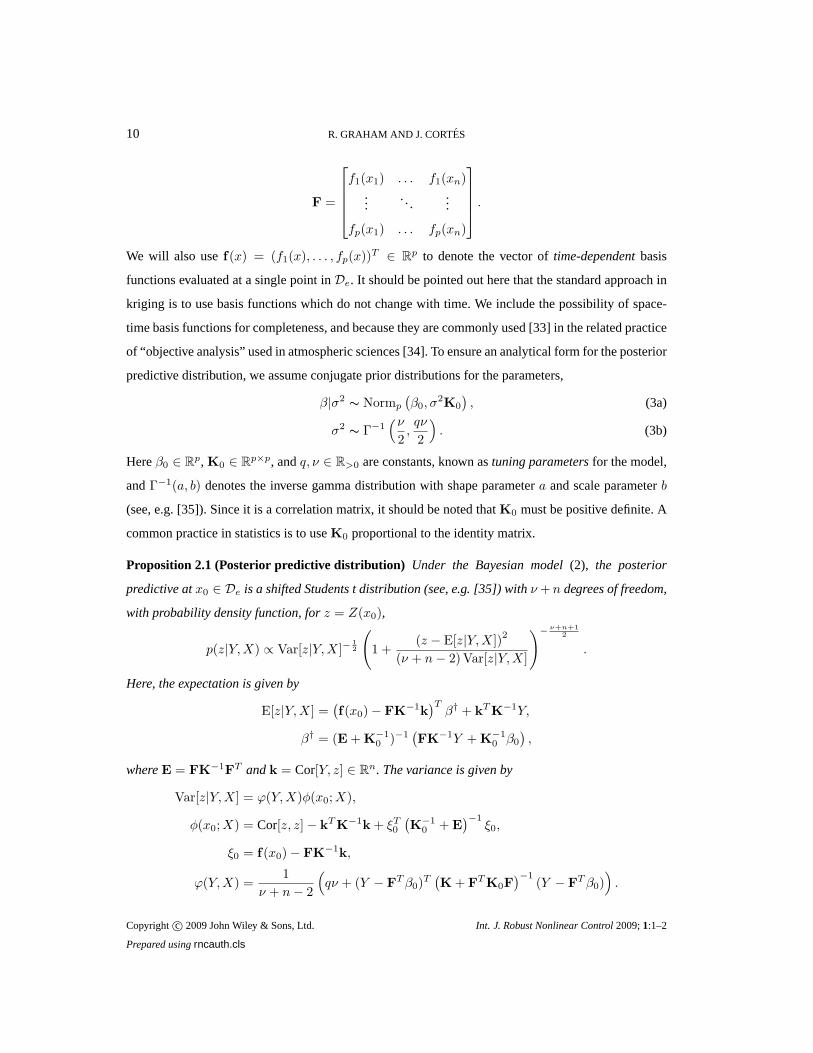
Proposition 2.1 (Posterior predictive distribution) Under the Bayesian model(2), the posterior
predictive atx0 ∈ De is a shifted Students t distribution (see, e.g. [35]) withν + n degrees of freedom,
with probability density function, forz = Z(x0),
p(z|Y,X) ∝ Var[z|Y,X]−12
(
1 +(z − E[z|Y,X])
2
(ν + n − 2) Var[z|Y,X]
)− ν+n+12
.
Here, the expectation is given by
E[z|Y,X] =(
f(x0) − FK−1
k)T
β† + kTK
−1Y,
β† = (E + K−10 )−1
(
FK−1Y + K
−10 β0
)
,
whereE = FK−1
FT andk = Cor[Y, z] ∈ R
n. The variance is given by
Var[z|Y,X] = ϕ(Y,X)φ(x0;X),
φ(x0;X) = Cor[z, z] − kTK
−1k + ξT
0
(
K−10 + E
)−1ξ0,
ξ0 = f(x0) − FK−1
k,
ϕ(Y,X) =1
ν + n − 2
(
qν + (Y − FT β0)
T(
K + FTK0F
)−1(Y − F
T β0))
.
Copyright c© 2009 John Wiley & Sons, Ltd. Int. J. Robust Nonlinear Control2009;1:1–2
Prepared usingrncauth.cls

COOPERATIVE ADAPTIVE SAMPLING OF RANDOM FIELDS WITH PARTIALLY KNOWN COVARIANCE 11
The proof of the proposition follows from the application ofBayes Theorem to the model given
by (3). Alternatively, it can also be derived from results in[4] and [25] using a technique similar to
the one used later in the proof of Proposition I.3 in AppendixI. Note that sinceK0 andK are positive
definite, the quantitiesφ(x0;X) andϕ(Y,X) are well posed.
Remark 2.2 (Terms in the posterior predictive variance) Note the form for the posterior predictive
variance in Proposition 2.1 as a product of two terms. The first term,ϕ(Y,X), is the posterior mean of
the parameterσ2, given the sampled data. We refer to it as thesigma mean. The second term,φ(x0;X),
can be thought of as the scaled posterior predictive variance conditioned onσ2. We refer to it as the
conditional variance. •
The conditional variance is very close to what the predictive variance would look like ifσ2 were
known, as we show next. The following result may be derived byapplying Bayes Theorem to the
model specified by (2) and (3a), withσ2 treated as known.
Proposition 2.3 (Kriging variance) If the variance parameterσ2 is known, the result is theuniversal
kriging predictor, and the posterior predictive variance takes the form,
VarUK[z|Y,X] = σ2(
Cor[z, z] − kTK
−1k + ξT
0 E−1ξ0
)
.
If, in addition, the mean of the field is known, the result is thesimple kriging predictor, and the posterior
predictive variance is given by,
VarSK[z|Y,X] = σ2(
Cor[z, z] − kTK
−1k)
.
Remark 2.4 (Extension of subsequent results to kriging) The simple and universal kriging results
are simplified versions of our overall model, and results from the rest of this paper may be applied
to those models with minimal modifications. An exception is that when approximatingVarUK using
subsets of measurements, care must be taken to ensure well-posedness. Specifically, an assumption that
n > p is required to ensure that the matrixE is nonsingular. •
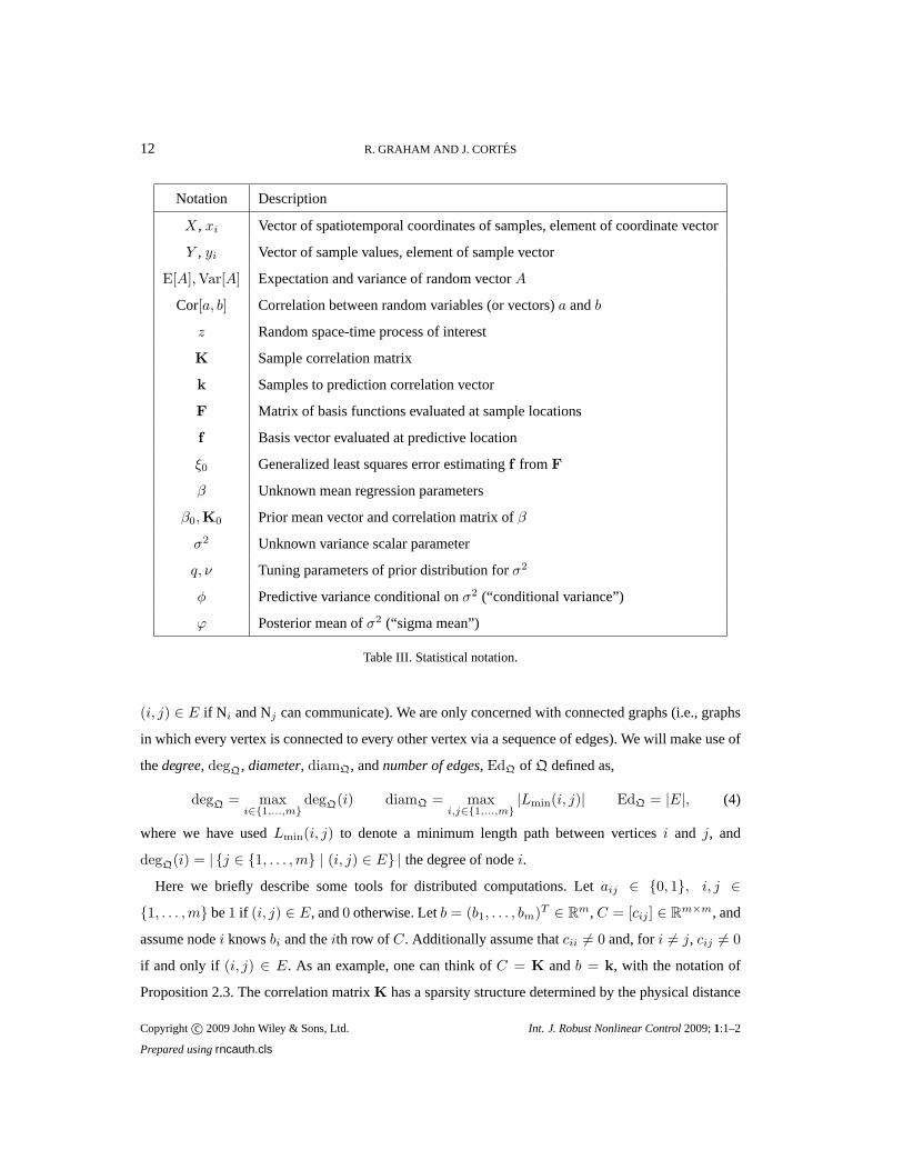
Table III provides an overview of notational conventions introduced in this section.
2.3. Tools for distributed computation
Consider a network,Q, of m nodes with limited communication capabilities. We writeQ = (N, E),
where N= (N1, . . . , Nm) denotes the vector of nodes, andE the set of communication edges (i.e.,
Copyright c© 2009 John Wiley & Sons, Ltd. Int. J. Robust Nonlinear Control2009;1:1–2
Prepared usingrncauth.cls
12 R. GRAHAM AND J. CORTES
Notation Description
X, xi Vector of spatiotemporal coordinates of samples, element of coordinate vector
Y , yi Vector of sample values, element of sample vector
E[A],Var[A] Expectation and variance of random vectorA
Cor[a, b] Correlation between random variables (or vectors)a andb
z Random space-time process of interest
K Sample correlation matrix
k Samples to prediction correlation vector
F Matrix of basis functions evaluated at sample locations
f Basis vector evaluated at predictive location
ξ0 Generalized least squares error estimatingf from F
β Unknown mean regression parameters
β0,K0 Prior mean vector and correlation matrix ofβ
σ2 Unknown variance scalar parameter
q, ν Tuning parameters of prior distribution forσ2
φ Predictive variance conditional onσ2 (“conditional variance”)
ϕ Posterior mean ofσ2 (“sigma mean”)
Table III. Statistical notation.
(i, j) ∈ E if N i and Nj can communicate). We are only concerned with connected graphs (i.e., graphs
in which every vertex is connected to every other vertex via asequence of edges). We will make use of
thedegree, degQ, diameter, diamQ, andnumber of edges, EdQ of Q defined as,
degQ = maxi∈1,...,m
degQ(i) diamQ = maxi,j∈1,...,m
|Lmin(i, j)| EdQ = |E|, (4)
where we have usedLmin(i, j) to denote a minimum length path between verticesi and j, and
degQ(i) = | j ∈ 1, . . . ,m | (i, j) ∈ E | the degree of nodei.
Here we briefly describe some tools for distributed computations. Let aij ∈ 0, 1, i, j ∈1, . . . ,m be1 if (i, j) ∈ E, and0 otherwise. Letb = (b1, . . . , bm)T ∈ R
m, C = [cij ] ∈ Rm×m, and
assume nodei knowsbi and theith row ofC. Additionally assume thatcii 6= 0 and, fori 6= j, cij 6= 0
if and only if (i, j) ∈ E. As an example, one can think ofC = K andb = k, with the notation of
Proposition 2.3. The correlation matrixK has a sparsity structure determined by the physical distance
Copyright c© 2009 John Wiley & Sons, Ltd. Int. J. Robust Nonlinear Control2009;1:1–2
Prepared usingrncauth.cls
COOPERATIVE ADAPTIVE SAMPLING OF RANDOM FIELDS WITH PARTIALLY KNOWN COVARIANCE 13
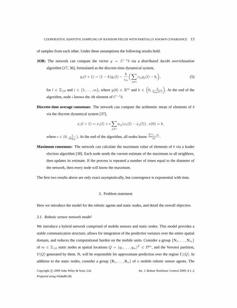
of samples from each other. Under these assumptions the following results hold.
JOR: The network can compute the vectory = C−1b via a distributed Jacobi overrelaxation
algorithm [17, 36], formulated as the discrete-time dynamical system,
yi(l + 1) = (1 − h)yi(l) −h
cii
(
∑
j 6=i
cijyj(l) − bi
)
, (5)
for l ∈ Z≥0 andi ∈ 1, . . . ,m, wherey(0) ∈ Rm andh ∈
(
0, 2λmax(C)
)
. At the end of the
algorithm, nodei knows theith element ofC−1b.
Discrete-time average consensus: The network can compute the arithmetic mean of elements ofb
via the discrete dynamical system [37],
xi(l + 1) = xi(l) + ǫ∑
j 6=i
aij(xi(l) − xj(l)), x(0) = b,
whereǫ ∈ (0, 1degQ
). At the end of the algorithm, all nodes knowPn
i=1 bi
m .
Maximum consensus: The network can calculate the maximum value of elements ofb via a leader
election algorithm [38]. Each node sends the current estimate of the maximum to all neighbors,
then updates its estimate. If the process is repeated a number of times equal to the diameter of
the network, then every node will know the maximum.
The first two results above are only exact asymptotically, but convergence is exponential with time.
3. Problem statement
Here we introduce the model for the robotic agents and staticnodes, and detail the overall objective.
3.1. Robotic sensor network model
We introduce a hybrid network comprised of mobile sensors and static nodes. This model provides a
stable communication structure, allows for integration ofthe predictive variance over the entire spatial
domain, and reduces the computational burden on the mobile units. Consider a groupN1, . . . , Nmof m ∈ Z>0 static nodes at spatial locationsQ = (q1, . . . , qm)T ∈ Dm, and the Voronoi partition,
V(Q) generated by them. Ni will be responsible for approximate prediction over the region Vi(Q). In
addition to the static nodes, consider a groupR1, . . . , Rn of n mobile robotic sensor agents. The
Copyright c© 2009 John Wiley & Sons, Ltd. Int. J. Robust Nonlinear Control2009;1:1–2
Prepared usingrncauth.cls

14 R. GRAHAM AND J. CORTES
robots take point samples of the spatial field at discrete instants of time inZ≥0. Our results below are
independent of the particular robot dynamics, so long as each agent is able to move up to a distance
umax ∈ R>0 between consecutive sampling times. Since the focus of thiswork is the online planning of
optimal sampling paths, any bounded delay incurred by network communication or calculations may
be incorporated into this maximum radius of movement between sampling instants. Bounds on such
delay may be inferred from the complexity analysis in Section 5.1. The communication radius of the
robots is alsorcom. If there is a chance that Rj will be within correlation range ofVi(Q) after moving
a distance ofumax (i.e., at the following sample time), then Ni must be able to communicate with Rj .
To that end, let
rcom ≥ maxi∈1,...,m
CR(Vi(Q)) + rs + umax. (6)
Among all the partitions ofD, the Voronoi partitionV(Q) ensures that (6) is satisfied with the smallest
communication radius. Figure 1 illustrates the communication requirements of the hybrid network.
The robots can sense the positions of other robots within a distance of2umax. At discrete timesteps,
N1
N2
N3
N4
R1
Figure 1. The static nodes are depicted as filled boxes, with the Voronoi partition boundaries as solid lines. Each
node can communicate with its Voronoi neighbors, and with any mobile robot within a distance ofrs+umax (dotted
circle) of the Voronoi cell (in the plot,N2 andN3 can communicate withR1).
each robot communicates the sample and spatial position to static nodes within communication
range, along with the positions of any other sensed robots. The nodes then compute control vectors,
and relay them back to robots within communication range. The implementation does not require
direct communication between robots. We refer to this hybrid network model asQhybrid, and the
communication network of just the nodes asQN. Note that bothQhybrid andQN are connected networks.
Copyright c© 2009 John Wiley & Sons, Ltd. Int. J. Robust Nonlinear Control2009;1:1–2
Prepared usingrncauth.cls

COOPERATIVE ADAPTIVE SAMPLING OF RANDOM FIELDS WITH PARTIALLY KNOWN COVARIANCE 15
3.1.1. Voronoi contraction for collision avoidanceIn addition to the maximum velocity and the
restriction toD, we impose a minimum distance requirementω ∈ R>0 between robots for collision
avoidance. Consider the spatial locationsP = (p1, . . . , pn) of then robotic agents at thekth timestep.
DefineΩ(k)i = (Vi(P ))ctn:ω/2 ∩B(pi, umax), where(Vi(P ))ctn:ω/2 denotes theω2 -contraction ofVi(P ).
For eachj 6= i ∈ 1, . . . , n, we havedist(Ω(k)i ,Ω
(k)j ) ≥ ω. Between timestepsk andk+1, we restrict
Ri to the regionΩ(k)i . Figure 2 shows an example inR2 of this set. The region of allowed movement of
umax R1
R2
R3
Ω(k)1
ω2
Figure 2. Example contraction regionΩ(k)1 (dashed) with Voronoi partition boundaries (solid) for comparison.
all robotic agents at timestepk ∈ Z≥0 is then the Cartesian product of the individual restrictions, i.e.,
Ω(k) =∏n
i=1 Ω(k)i ⊂ (Rd)n. Note that eachΩ(k)
i is the intersection of sets which are closed, bounded,
and convex, and hence inherits these properties, which are in turn also inherited byΩ(k). Further note
that computation of the Voronoi partition generated by all robots is not required, only the partition
boundaries between adjacent robots separated by less than2umax. We assume that the regionΩ(k)i is
reachable between stepsk andk + 1. For vehicles with restricted dynamics, minimal modifications
allow extension of these results to any nonempty, convex subset ofΩ(k)i .
3.2. The average variance as objective function
For predictions over a spatiotemporal region, the average variance is a natural measure of uncertainty.
Using Proposition 2.1, we define the average over the region of the posterior predictive variance,
A = ϕ(Y,X)
∫
D
∫
T
φ((s0, t0);X) dt0 ds0. (7)
Copyright c© 2009 John Wiley & Sons, Ltd. Int. J. Robust Nonlinear Control2009;1:1–2
Prepared usingrncauth.cls

16 R. GRAHAM AND J. CORTES
Here,Y ∈ (Rn)kmax is a sequence of samples taken at discrete times1, . . . , kmax, kmax ∈ Z>0,
at space-time locationsX ∈ (Dne )
kmax. We takeT = [1, kmax] to be the time interval of interest,
indicating that the goal of the experiment is to develop an estimate of the space-time process over the
entire duration. Other time intervals may be of interest in different experiments. Their use follows with
minimal changes to the methods described here.
One would like to choose the sample locations that minimizeA. Since samples are taken
sequentially, with each new set restricted to a region nearby the previous, and since the sigma mean
depends on the actual values of the samples, one cannot simply optimize over(Dne )kmax a priori.
Consider, instead, a greedy approach in which we use past samples to choose the positions for the next
ones. At each timestep we choose the next locations to minimize the average posterior variance of the
predictor given the data known so far. In Section 4, we develop a sequential formulation of the average
posterior predictive variance and discuss its amenabilityto distributed implementation overQhybrid.
4. Distributed criterion for adaptive design
In this section we develop an optimality criterion to maximally reduce the average predictive variance
at each timestep. We begin by introducing some notation thatwill help us make the discussion precise.
Let Y (k) ∈ Rn, k ∈ 1, . . . , kmax, denote the samples taken at timestepk, at space-time positions
X(k) ∈ Dne . LetY (k1:k2) =
(
Y (k1), . . . , Y (k2))
∈ Rn(k2−k1+1), k1 < k2, denote the vector of samples
taken over a range of timesteps, at positionsX(k1:k2) =(
X(k1), . . . ,X(k2))
∈ Dn(k2−k1+1)e . At stepk,
the samplesY (1:k) have already been taken. We are interested in choosing spatial locations,P ∈ Ω(k),
at which to take the next samples. To that end, letX(1:k+1) : Ω(k) → Dn(k+1)e map a new set of
spatial locations to the vector of spatiotemporal locations which will result if the(k +1)th samples are
taken there, i.e.,X(1:k+1)(P ) =(
X(1:k), (P, k + 1))
. The adaptive design approach is then to use the
samples that minimize the average prediction varianceso far,
A(k)(P ) = ϕ(
Y (1:k+1),X(1:k+1)(P ))
∫
D
∫
T
φ(
(s0, t0);X(1:k+1)(P )
)
dt0 ds0. (8)
This sequential formulation of the problem allows us to use past measurements without worrying about
the ones at steps afterk+1. However, efficient distributed implementation still suffers from three major
obstacles. First, the spatially distributed nature of the problem implies that not all sample locations are
accessible to any given agent at any given time. Second, inversion of then(k+1)×n(k+1) correlation
Copyright c© 2009 John Wiley & Sons, Ltd. Int. J. Robust Nonlinear Control2009;1:1–2
Prepared usingrncauth.cls

COOPERATIVE ADAPTIVE SAMPLING OF RANDOM FIELDS WITH PARTIALLY KNOWN COVARIANCE 17
matrix, which grows withk2, quickly becomes an unreasonable burden. Finally, the sigma mean also
depends on the actual values of the samples at stepk +1, which are not known until the measurements
are taken. We handle these problems through a series of approximations, first to the conditional variance
in Section 4.1, then to the sigma mean in Section 4.2, resulting in an approximation of the value ofA(k)
which is both distributed in nature and computationally efficient.
4.1. Upper bound on conditional variance
We seek an efficient approximation of the conditional variance termφ(
(s0, t0);X(1:k+1)(P )
)
in (8). As
noted in Remark 2.2,φ represents the direct effect of the sample locations on the predictive uncertainty
(i.e., conditional onσ2). The network of static nodes provides a convenient method for calculating the
spatial average. The average over the entire region may simply be written as the sum of averages over
each cell in the Voronoi partition generated by the static nodes. As those samples which are spatially
near a given cell have the most influence on reducing the variance of predictions there, we consider
using local information onlyin these regional calculations. Likewise, the interactionbetween current
samples and those far in the past is minimal, and we restrict attention to recent timesteps to avoid
the problem of growing complexity. The following result gives an approximation of the integrated
conditional variance which may be calculated byQN based on local information only.
Proposition 4.1 (Approximate integrated conditional variance) LetX(k+1−⌊rt⌋:k+1)j (P ) denote an
ordering of the set of past or current space-time locations correlated in space toVj(Q) and in time to
k + 1 such that
iF
(
X(k+1−⌊rt⌋:k+1)j (P )
)
=
(s, t) ∈ iF
(
X(1:k+1)(P ))
| dist(s, Vj(Q)) < rs andk + 1 − t < rt
.
Let φ(k)j : De × Ω(k) → R map a prediction locationx0 ∈ De and a vector of potential spatial
locations to sampleP ∈ Ω(k) to the conditional variance of a prediction made atx0 using only the
samples at space-time locationsX(k+1−⌊rt⌋:k+1)j (P ). Then the following holds,
∫
D
∫
T
φ((s0, t0);X(1:k+1)(P )) dt0 ds0 ≤
m∑
j=1
∫
Vj(Q)
∫
T
φ(k)j ((s0, t0);P ) dt0 ds0.
Proof. Note that althoughX(k+1−⌊rt⌋:k+1)j (P ) is not unique, the invariance of the conditional variance
to permutations of the sample locations ensures uniquenessof φj
(
x0;P)
. The result follows from
Proposition I.2 in Appendix I.
Copyright c© 2009 John Wiley & Sons, Ltd. Int. J. Robust Nonlinear Control2009;1:1–2
Prepared usingrncauth.cls

18 R. GRAHAM AND J. CORTES
4.2. Approximate sigma mean
In this section, we describe our approach to deal with the sigma mean termϕ(Y (1:k+1),X(1:k+1)(P ))
in (8). Note that the effect of the sigma mean on prediction isindirect, and its value has the same
influence on predictions regardless of the predictive location. As such, we do not use spatially local
approximations as we did for the conditional variance. However, to avoid the problem of complexity
growth, we use samples from only a subset of the timesteps. Wediscuss this next. Subsequently, we
address the issue of unrealized sample values by using a generalized least squares estimate.
4.2.1. Incorporating new data.Here we consider approximating the value ofϕ as calculated with
samples from a subset of timesteps. There are various reasons for using different sample subsets
depending on the field under study, the objectives of the experiment, and the desired accuracy of
optimization. Sinceϕ is invariant under permutations of the sample vector, the specific ordering is
irrelevant. Proposition 4.2 serves as the basis for choosing the samples to include in an approximation
of the sigma mean. The proof follows from (9c) in Lemma I.3 in Appendix I.
Proposition 4.2 (Approximate sigma mean) LetY1 ∈ Rn1 andY2 ∈ R
n2 denote two sample vectors
of lengthsn1, n2 ∈ Z>0, and letY = (Y1, Y2). Letϕ2 = E[σ2|Y2] denote the value of the sigma mean
conditional on only the samples inY2, andϕ = E[σ2|Y ] the value conditional on the whole sample
vectorY . Then,
ϕ = ϕ2
( ν + n2 − 2
ν + n1 + n2 − 2+
(Y1 − E[Y1|Y2])T Var[Y1|Y2]
−1(Y1 − E[Y1|Y2])
ν + n1 + n2 − 2
)
,
whereE[Y1|Y2] and Var[Y1|Y2] denote the conditional expectation and variance, respectively, ofY1
givenY2 (see Proposition I.1 in Appendix I).
This result contains some important implications with respect to the optimization problem. First,
if we use the full value ofϕ(Y (1:k),X(1:k)(P )) = E[σ2|Y (1:k)] in our optimality metric at each
timestep, and all steps are optimized with respect to this measure, the new information gained at later
steps diminishes significantly, while the amount of effort required to glean that information increases.
Second, the additional information added by includingY1 is directly related to how wellY1 may be
estimated fromY2.
These observations lead us to suggest the following three strategies for choosing samples to use in
the approximation of the sigma mean.
Copyright c© 2009 John Wiley & Sons, Ltd. Int. J. Robust Nonlinear Control2009;1:1–2
Prepared usingrncauth.cls

COOPERATIVE ADAPTIVE SAMPLING OF RANDOM FIELDS WITH PARTIALLY KNOWN COVARIANCE 19
Exploration-exploitation: The diminishing returns suggest using an exploration-exploitation
approach [27]. Here a block oftblk ∈ 1, . . . , kmax sample steps at the beginning of the
experiment designates an exploration phase, during which the sigma mean is taken into account
in the optimization. Subsequent iterations constitute an exploitation phase in which the sigma
mean is treated as a fixed constant and we optimize only the conditional variance.
Recent block: The second strategy is to always use the most recenttblk sample steps. This increases
the computational burden over the exploration-exploitation approach, but ensures that each step
takes the unknown covariance into account in optimization.
Block update: A third choice is to use select blocks oftblk timesteps for scheduled updates of the
sigma mean. Lettskip ∈ Z>0 be a fixed number of timesteps to skip between updates. The
advantage of this method in reducing computational complexity comes from an assumption that
tskip > ⌈rt⌉ − 1, resulting in a block diagonal correlation matrix.
These three approximation methods trade off computationalcomplexity for accuracy. The
appropriateness of each method depends on the specific requirements of the scenario. In all three cases,
the maximum size of the correlation matrix which must be inverted isntblk ×ntblk. Furthermore, using
Lemma I.3, it can be seen that this matrix inversion is the most computationally intensive part of
calculating the sigma mean. Therefore, using any one of these three methods, we avoid computational
complexities which grow out of proportion to the information gain. However, we still have the problem
that the sigma mean includes sample values which have not been taken yet. We address this issue in the
next section. To avoid unnecessary notation, we assume throughout the sequel that all available samples
are used to calculateϕ(k). To accommodate the approximations outlined in this section, it is necessary
only to replace them with the subsampled ones, and modify thenumber of samples accordingly.
4.2.2. Approximating unrealized sample values.While seeking to optimize the(k + 1)th set of
measurements, we would like to incorporate the effect of their locationson the posterior variance,
but the actual values have not yet been sampled. Our approachis to use a generalized least squares
approximation ofY (k+1). We describe this in detail in the next result whose proof is in Appendix I.
Proposition 4.3 (Generalized least squares estimate of sigma mean) Let Y(k)
LS : Ω(k) → Rn map
a vector of spatial locationsP ∈ Ω(k) to the generalized least squares estimate, based on the
Copyright c© 2009 John Wiley & Sons, Ltd. Int. J. Robust Nonlinear Control2009;1:1–2
Prepared usingrncauth.cls

20 R. GRAHAM AND J. CORTES
sample vectorY (1:k), of a vector of samples to be taken at space-time positions(P, k + 1). Let
ϕ(k+1) : Ω(k) → R be defined by,
ϕ(k+1)(P ) =1
ν + n(k + 1) − 2
[
qν + βT0 K
−10 β0 + Υ(k)
−(
K−10 β0 + Γ(k)
)T (K
−10 + E
(k+1)(P ))−1(
K−10 β0 + Γ(k)
)
]
, where
Υ(k) = (Y (1:k))T (K(1:k))−1Y (1:k), Γ(k) = F(1:k)(K(1:k))−1Y (1:k),
and E(k+1)(P ) denotes the matrixE as calculated with space-time location vectorX(k+1)(P ) =
(
X(1:k), (P, k + 1))
. After the new samples,Y (k+1) have been taken at locations(P, k + 1), let
y(k)LS : Ω(k) → R
n denote the estimation error, i.e.,y(k)LS (P ) = Y (k+1) − Y
(k)LS (P ). Then,
ϕ(k+1) =ϕ(k)(y
(k)LS (P ) − 2µk+1|≤k)T Var[Y (k+1)|Y (1:k)]−1
ν + n(k + 1) − 2y(k)LS (P ) + ϕ(k+1)(P ), where
µk+1|≤k = (F(k+1) − F(1:k)(K(1:k))−1Cor[Y (1:k), Y (k+1)])T
× (E(1:k) + K−10 )−1
(
F(1:k)(K(1:k))−1Y (1:k) + K
−10 β0
)
.
In other words,ϕ(k+1) may be estimated byϕ(k+1)(P ). The estimation is exact ifY (k+1) =
Y(k)
LS (P ).
Remark 4.4 (Quality of estimation) It should be pointed out here that the generalized least squares
estimate is not the best guess of the value of the unrealized data. That would correspond to the
conditional expectation given all past data. However, fromProposition 4.2, we can see that this choice
would result in zeroing out the influence of the locations on the posterior mean ofσ2. Instead, we use
an optimality criterion which accounts for this influence. •
4.3. The aggregate average prediction variance and its smoothness properties
Building on the results from Sections 4.1 and 4.2, we define here theaggregate average prediction
varianceA(k). Unlike A(k), the functionA(k) may be computed efficiently in a distributed manner
over the networkQhybrid. The following result is a direct consequence of Propositions 4.1 and 4.3.
Proposition 4.5. (Spatiotemporal approximation for distributed implementation) Let A(k)j :
Ω(k) → R be defined by
A(k)j (P ) = ϕ(k+1)(P )
∫
Vj(Q)
∫
T
φ(k)j ((s, t), P ) dt ds.
Copyright c© 2009 John Wiley & Sons, Ltd. Int. J. Robust Nonlinear Control2009;1:1–2
Prepared usingrncauth.cls
COOPERATIVE ADAPTIVE SAMPLING OF RANDOM FIELDS WITH PARTIALLY KNOWN COVARIANCE 21
Under the assumption that the error term from Proposition 4.3 satisfies,
limk→∞
ϕk(y(k)LS (P ) − 2µk+1|≤k)T Var[Y (k+1)|Y (1:k)]−1
ν + n(k + 1) − 2y(k)LS (P ) = 0,
thenA(k)(P ) =m∑
j=1
A(k)j (P ) satisfies lim
k→∞A(k)(P ) ≥ lim
k→∞A(k)(P ).
Next, we characterize the smoothness properties ofA(k). Let∇il denote the partial derivative with
respect topil, the lth spatial component of the spatial position of Ri. We denote by∇i the partial
derivative with respect topi, i.e.,∇i = (∇i1, . . . ,∇id)T . Thus the gradient ofA(k) at locationP may
be represented as thend-dimensional vector(
∇T1 A(k)(P ), . . . ,∇T
n A(k)(P ))T
. Given a matrixA,
denote by∇ilA the component-wise partial derivative ofA. The proof of the next result amounts to a
careful bookkeeping of the smoothness properties of the various ingredients in the expressions.
Lemma 4.6 (Gradient of conditional variance) If f1, . . . , fp are C1 with respect to the spatial
position of their arguments, then the mapP 7→ φ(k)j (x0, P ) is C1 onΩ(k) with partial derivative,
∇ilφ(k)j (x0, P ) = −2kT
K−1∇ilk + k
TK
−1∇ilKK−1
k
− ξT0
(
K−10 + E
)−1 ∇ilE(
K−10 + E
)−1ξ0 + 2ξT
0
(
K−10 + E
)−1 ∇ilξ0, with
∇ilξ0 = −∇ilFK−1
k − FK−1∇ilk + FK
−1∇ilKK−1
k,
∇ilE = ∇ilFK−1
FT + FK
−1∇ilFT − FK
−1∇ilKK−1
F,
where the matricesK, E, andF and the vectorsk, andξ0 are calculated from the space-time location
subvector,X(k+1−⌊rt⌋:k+1)j (P ).
If, in addition, the partial derivatives off1, . . . , fp areC1 with respect to the spatial position of their
arguments, then the mapP 7→ ∇iφ(k)j (x0, P ) is globally Lipschitz onΩ(k).
It is worth noting that the matrix∇ilF is nonzero only in columni. The matrix∇ilK is nonzero
only in row and columni. Additionally, due to the finite correlation range in space and time, only
those elements corresponding to correlation with other measurement locationsx = (s, t) which satisfy
‖pi − s‖ ≤ rs andt > k + 1 − rt are nonzero.
Note that the value ofϕ(k+1)(P ) depends onP only through the matrixE(k+1)(P ), whose
partial derivative is analogous to that ofE in Lemma 4.6. If subsampling is used to approximateϕ
per Section 2.1, we set∇ϕ(k+1)(P ) = 0 for those steps which are skipped. Here we assume no
subsampling for notational convenience. This leads us to the following result.
Copyright c© 2009 John Wiley & Sons, Ltd. Int. J. Robust Nonlinear Control2009;1:1–2
Prepared usingrncauth.cls

22 R. GRAHAM AND J. CORTES
Lemma 4.7 (Gradient of sigma mean) If f1, . . . , fp are C1 with respect to the spatial position of
their arguments, thenϕ(k+1) is C1 onΩ(k) with partial derivative,
∇ilϕ(k+1)(P ) = −Ψ(P )T ∇ilE
(k+1)(P )Ψ(P )
ν + n(k + 1) − 2, where
Ψ(P ) =(
K−10 + E
(k+1)(P ))−1(
K−10 β0 + Γ(k)
)
.
Additionally, if the partial derivatives off1, . . . , fp areC1 with respect to the spatial position of their
arguments, the gradient∇ϕ(k+1) is globally Lipschitz onΩ(k).
We are now ready to state the smoothness properties ofA(k) and provide an explicit expression for
its gradient. This is a direct consequence of the lemmas above.
Proposition 4.8 (Gradient of approximate average variance) If f1, . . . , fp are C1 with respect to
the spatial position of their arguments, thenA(k) is C1 onΩ(k) with partial derivative,
∇iA(k)(P ) = ϕ(k+1)(P )
∫
Vj(Q)
∫
T
∇iφ(k)j ((s, t), P ) dt ds
+ ∇iϕ(k+1)(P )
∫
Vj(Q)
∫
T
φ(k)j ((s, t), P ) dt ds.
Additionally, if the partial derivatives off1, . . . , fp areC1 with respect to the spatial position of their
arguments, the gradient∇A(k) is globally Lipschitz onΩ(k).
4.4. Distributed computation of aggregate average prediction variance and its gradient
Here, we substantiate our assertion that the aggregate average prediction variance and its gradient
introduced in Section 4.3 are distributed over the networkQhybrid. SinceV(Q) is a partition of the
physical space, we may partition all sample locations spatially by region. Thus for each(s, t) ∈ iF(X),
there is exactly onej ∈ 1, . . . ,m such thats ∈ Vj(Q). In order for the network to calculateA(k)
and its gradient atP , it is sufficient for Nj to computeA(k)j and∇iA(k)
j for each robot inVj(Q).
ThenA(k) may be calculated via discrete-time average consensus (cf.Section 2.3), while∇iA(k) may
be calculated from information local to Ri. From Propositions 4.5 and 4.8, it can be seen that the
calculation ofA(k)j and∇iA(k)
j requires only local information in addition to the (global)values of
ϕ(k+1)(P ) and∇iϕ(k+1)(P ). Let us explain how these two quantities can be calculated.
For i ∈ 1, . . . , nk, let x(1:k)i andy
(1:k)i denote theith element of the vectorX(1:k) andY (1:k),
respectively. Let I(k)Local : Z>0 → F(Z>0) map the index of the node to the set of indices of samples
Copyright c© 2009 John Wiley & Sons, Ltd. Int. J. Robust Nonlinear Control2009;1:1–2
Prepared usingrncauth.cls

COOPERATIVE ADAPTIVE SAMPLING OF RANDOM FIELDS WITH PARTIALLY KNOWN COVARIANCE 23
whose spatial position lies inside its Voronoi cell, and whose time element is correlated to timek + 1,
I(k)Local(j) =
i ∈ 1, . . . , nk | x(1:k)i = (s, t) ands ∈ Vj(Q)
With a slight abuse of notation, define I(k+1)Local (j, P ) to be the equivalent set of indices into the full vector
of space-time measurement locations,X(k+1)(P ).
In the following results, we assume that a desired level of accuracy is known a priori to all nodes
so that an execution of the JOR or average consensus algorithms have a finite termination criterion.
Unless stated otherwise, the executions of these algorithms may take place in serial or parallel. Our
first result illustrates how the network can calculate the terms inϕ(k+1)(P ) which do not depend onP .
Proposition 4.9 (Distributed calculations without P ) for j ∈ 1, . . . ,m, assume thatNj knows
x(1:k)i , y
(1:k)i for eachi ∈ I(k)
Local(j). After p + 1 executions of the JOR algorithm and two subsequent
consensus algorithms,Nj has access to,
#1: elementi of (K(1:k))−1Y (1:k) ∈ R, i ∈ I(k)Local(j) via JOR;
#2: coli(
F(1:k)(K(1:k))−1
)
∈ Rp, i ∈ I(k)
Local(j) via JOR;
#3: Γ(k) ∈ Rp via consensus;
#4: Υ(k) ∈ Rp via consensus.
Proof. Under the assumptions onQhybrid, the matrixK(1:k), satisfies the requirements of the distributed
JOR algorithm. The results here build on this fact and the connectedness ofQN (which allows for
consensus).
Next, we describe calculations that the network can executewhen robotic agents are at locationsP .
Proposition 4.10 (Distributed calculations with P ) Given P ∈ Ω(k), assume thatNj , for j ∈1, . . . ,m, knowsx(1:k)
i for eachi ∈ I(k+1)Local (j, P ) and the results of Proposition 4.9. LetF
(k+1)(P )
denote the matrix of basis functions evaluated at locationsX(1:k+1)(P ). Afterp executions of JOR andp(p+1)
2 executions of consensus algorithms,Nj has access to,
#5: coli(
F(k+1)(P )(K(k+1)(P ))−1
)
∈ Rp, i ∈ I(k+1)
Local (j, P ) via JOR;
#6: E(k+1)(P ) ∈ R
p×p via consensus.
After these computations,Nj can calculate∇ilE(k+1) for l ∈ 1, . . . , d, and consequentlyϕ(k+1)(P )
and∇iϕ(k+1)(P ) for each robot ini ∈ 1, . . . , n | pi ∈ Vj(Q).
Copyright c© 2009 John Wiley & Sons, Ltd. Int. J. Robust Nonlinear Control2009;1:1–2
Prepared usingrncauth.cls
24 R. GRAHAM AND J. CORTES
Proof. The matrixK(k+1)(P ) satisfies the requirements of the distributed JOR algorithmby the
assumptions onQhybrid. The itemized results follow from this, and the symmetry of the matrix
E(k+1)(P ). The calculation ofϕ(k+1) and partial derivatives follow from Lemmas I.3 and 4.7.
5. Distributed optimization of the aggregate average predictive variance
Here we present a distributed algorithm which is guaranteedto converge to a stationary point ofA(k)
on Ω(k). The DISTRIBUTED PROJECTEDGRADIENT DESCENT ALGORITHM in Table V allows the
network of static nodes and mobile agents to find local minimaof A(k) on Ω(k). At timestepk, the
nodes follow a gradient descent algorithm, defining a sequence of configurations,P †l , l ∈ Z>0, with
P†1 = P (k) ∈ Ω(k), the vector of current spatial locations of the robotic agents and
P†l+1 = projΩ
(
P†l − α∇A|P †
l
)
, α ∈ R≥0,
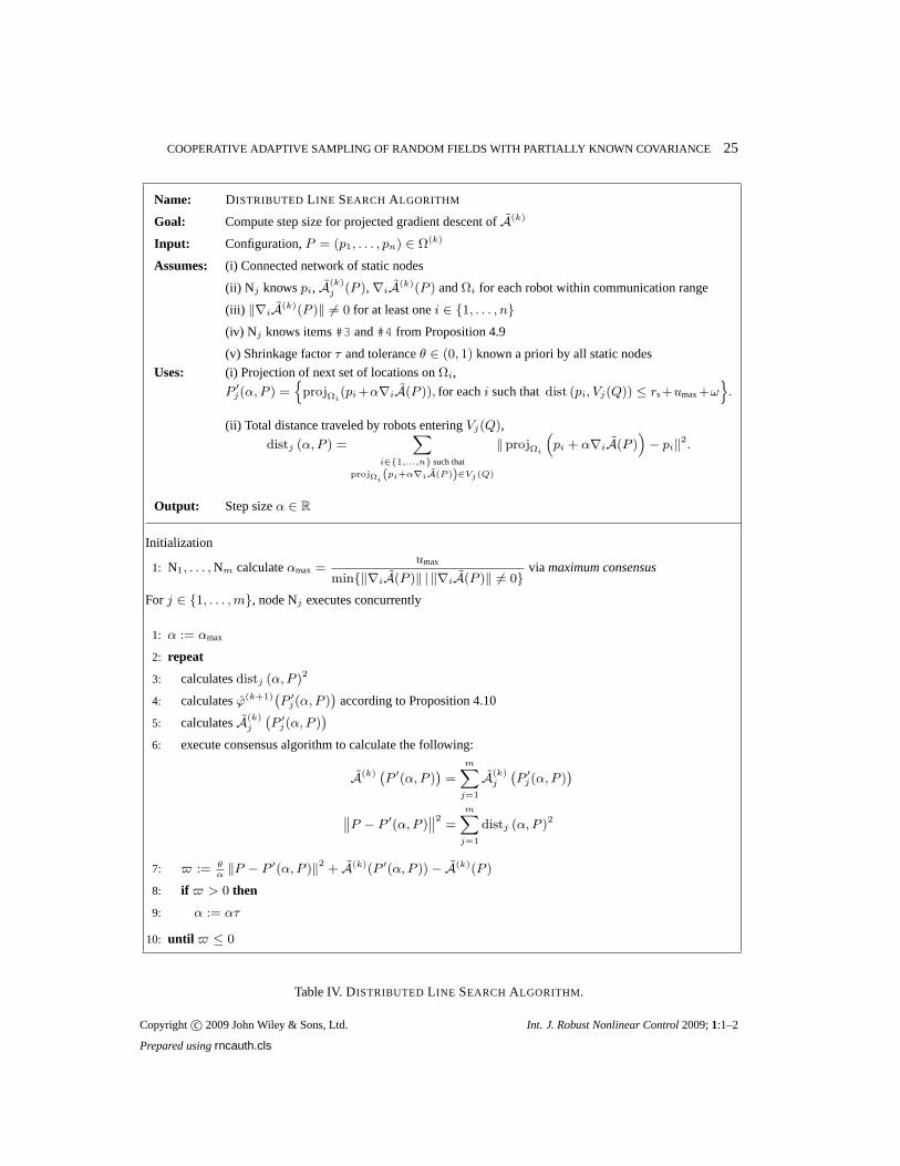
whereα is chosen via the DISTRIBUTED L INE SEARCH ALGORITHM outlined in Table IV. The
DISTRIBUTED L INE SEARCH ALGORITHM is a distributed version of the LINE SEARCH ALGORITHM
from Table II. The maximum stepsize,αmax ∈ R>0, is designed to ensure that all robots with nonzero
partial derivatives can move the maximum distance.
When|A(k)(P †l+1)−A(k)(P †
l )| = 0, the algorithm terminates, and the nodes setP (k+1) = P†l+1. By
the end of this calculation, each node knows the identity of robotic agents in its Voronoi cell at timestep
k + 1. Node Nj transmitspi(k + 1) to robot Ri, which then moves to the location between timesteps.
Note that although each robot may be sending position and sample information to multiple nodes, the
approximate average prediction variance is calculatedwithin the Voronoi cell. As the Voronoi cells do
not overlap, there is no problem with information repetition.
The following result describes some nice properties of the DISTRIBUTED PROJECTEDGRADIENT
DESCENT ALGORITHM. Its proof is a direct result of the construction of the algorithm and the fact
that it is equivalent to a centralized projected gradient descent.
Proposition 5.1. (Properties of the DISTRIBUTED PROJECTED GRADIENT DESCENT ALGO-
RITHM) TheDISTRIBUTED PROJECTEDGRADIENT DESCENTALGORITHM is distributed over the
networkQhybrid. Moreover, if the partial derivatives off1, . . . , fp are C1 with respect to the spatial
position of their arguments, any execution is such that the robots do not collide and, at each timestep
after the first, measurements are taken at stationary configurations ofP 7→ A(k)(P ) overΩ(k).
Copyright c© 2009 John Wiley & Sons, Ltd. Int. J. Robust Nonlinear Control2009;1:1–2
Prepared usingrncauth.cls
COOPERATIVE ADAPTIVE SAMPLING OF RANDOM FIELDS WITH PARTIALLY KNOWN COVARIANCE 25
Name: DISTRIBUTED L INE SEARCH ALGORITHM
Goal: Compute step size for projected gradient descent ofA(k)
Input: Configuration,P = (p1, . . . , pn) ∈ Ω(k)
Assumes: (i) Connected network of static nodes
(ii) N j knowspi, A(k)j (P ), ∇iA
(k)(P ) andΩi for each robot within communication range
(iii) ‖∇iA(k)(P )‖ 6= 0 for at least onei ∈ 1, . . . , n
(iv) Nj knows items#3 and#4 from Proposition 4.9
(v) Shrinkage factorτ and toleranceθ ∈ (0, 1) known a priori by all static nodes
Uses: (i) Projection of next set of locations onΩi,
P′j(α, P ) =
n
projΩi(pi +α∇iA(P )), for eachi such thatdist (pi, Vj(Q)) ≤ rs+umax+ω
o
.
(ii) Total distance traveled by robots enteringVj(Q),
distj (α, P ) =X
i∈1,...,n such that
projΩi(pi+α∇iA(P ))∈Vj(Q)
‖projΩi
“
pi + α∇iA(P )”
− pi‖2.
Output: Step sizeα ∈ R
Initialization
1: N1, . . . , Nm calculateαmax =umax
min‖∇iA(P )‖ | ‖∇iA(P )‖ 6= 0via maximum consensus
For j ∈ 1, . . . , m, node Nj executes concurrently
1: α := αmax
2: repeat
3: calculatesdistj (α, P )2
4: calculatesϕ(k+1)`
P ′j(α, P )
´
according to Proposition 4.10
5: calculatesA(k)j
`
P ′j(α, P )
´
6: execute consensus algorithm to calculate the following:
A(k) `
P′(α, P )
´
=
mX
j=1
A(k)j
`
P′j(α, P )
´
‚
‚P − P′(α, P )
‚
‚
2=
mX
j=1
distj (α, P )2
7: := θα‖P − P ′(α, P )‖
2+ A(k)(P ′(α, P )) − A(k)(P )
8: if > 0 then
9: α := ατ
10: until ≤ 0
Table IV. DISTRIBUTED L INE SEARCH ALGORITHM.
Copyright c© 2009 John Wiley & Sons, Ltd. Int. J. Robust Nonlinear Control2009;1:1–2
Prepared usingrncauth.cls

26 R. GRAHAM AND J. CORTES
Name: DISTRIBUTED PROJECTEDGRADIENT DESCENTALGORITHM
Goal: Find a local minimum ofA(k) within Ω(k).
Assumes: (i) Connected network of static computing nodes and mobile robotic sensingagents
(ii) Static nodes deployed overD such thatrcom ≥ maxi∈1,...,m CR(Vi(Q)) + rs + umax,
robotic agents in initial configurationP (1) ∈ Ω(k)
(iii) Line search shrinkage factorτ and tolerance valueθ ∈ (0, 1) known a priori by all nodes
(iv) A termination marker known to all nodes and robots which may be sent to mark the end of a
gradient descent loop.Uses: (i) Each node uses the temporary vectorsPcur, respectivelyPnext to hold the configuration at the
current, respectively next step of the gradient projection algorithm. For ease of exposition, we use
global notation although Nj only calculates and uses the parts of these vectors which correspond
to agents currently within communication range.
At time k ∈ Z≥0, node Nj executes:
1: setsRcov(j) := Ri | dist(pi(k), Vj(Q)) ≤ rs
2: collectsy(k)i andpi(k) from Ri for eachi ∈ Rcov(j)
3: computesA(k)j
`
P (k)´
, thenA(k)`
P (k)´
by consensus
4: setsPnext := P (k)
5: repeat
6: setsPcur := Pnext(j) and calculates−∇A(k)j |Pcur
7: transmits∇iA(k)j (Pcur) to robots inRcov(j)
8: collects sum∇iA(k)(Pcur) from robots inRcov(j)
9: runs DISTRIBUTED L INE SEARCH ALGORITHM at
Pcur to getα
10: setsPnext := Pcur + α∇A(k)|Pcur
11: calculates|A(k)(Pnext) − A(k)(Pcur)|
12: until |A(k)(Pnext) − A(k)(Pcur)| = 0
13: setsP (k+1) := Pnext, sends position to robots inVj(Q)
Meanwhile, robot Ri executes:
1: setsScov(i) := Nj | dist(pi(k), Vj(Q))≤ rs
2: takes measurementy(k)i atpi(k)
3: sendsy(k)i andpi(k) to nodes inScov(i)
4: repeat
5: receives∇iA(k)j (P (k)) from nodes inScov(i)
6: calculates sum∇iA(k)(P (k))
7: sends∇iA(k)(P (k)) to all nodes inScov(i)
8: until receives finish marker from any node
9: receives locationpi(k + 1) and moves to it
Table V. DISTRIBUTED PROJECTEDGRADIENT DESCENTALGORITHM.
Copyright c© 2009 John Wiley & Sons, Ltd. Int. J. Robust Nonlinear Control2009;1:1–2
Prepared usingrncauth.cls

COOPERATIVE ADAPTIVE SAMPLING OF RANDOM FIELDS WITH PARTIALLY KNOWN COVARIANCE 27
The proposed algorithm is robust to failures in themobileagents. If an agent stops sending position
updates, it ceases to receive new control vectors. The rest of the network continues operating with the
available resources and will eventually sample the areas previously covered by the failing agents. With
minor modifications, the algorithm could be made robust to a certain number of node failures as well.
However, this would require larger communication radius and extra storage (essentially having each
node keep track of the sample locations stored by its Voronoineighbors).
Remark 5.2 (Extension to relative positioning) It is interesting to observe that, due to the fact that
the actual positions of samples are only required in a local context, our algorithm can also be
implemented in a robotic network with relative positioning. The only requirements are the following:
that each node can calculate the mean basis function for all local samples; that each node can calculate
the correlations between pairs of local samples and that neighboring nodes can agree on the ordering
of those samples within the global matrix. These modifications would not impact the convergence
properties of the algorithm. •
5.1. Complexity analysis
Here we examine in detail the complexity of the DISTRIBUTED PROJECTEDGRADIENT DESCENT
ALGORITHM in terms of the number of robotic agents and static nodes. Forreference, we compare
it against a centralized strategy that uses all-to-all broadcast and global information, and does not
take advantage of the distributed nature of the problem. In order to avoid complexities which grow
unbounded withk, we assume here that one of the approximation methods is employed for calculating
ϕ as outlined in Section 4.2.1. For the purposes of complexity, it does not matter which method is used,
only that the size of the matrix which must be inverted at any step is bounded byntblk, and thus does
not depend onk. Letn(k)c ∈ 1, . . . , ntblk denote the number of samples used in thecurrentblock for
approximatingϕ at stepk, and letK(k)c denote the correlation matrix of those samples.
Given that the DISTRIBUTED PROJECTEDGRADIENT DESCENT ALGORITHM is sequential, and
designed to run for a fixed number of timesteps, we are concerned here with complexities involved in
performing a single step. Below, where we refer to complexity notions over multiple iterations of an
algorithm, we are considering the nested algorithms such asJOR, or consensus, which run during a
single step of the DISTRIBUTED PROJECTEDGRADIENT DESCENTALGORITHM.
We examine the algorithm performance against the followingnotions of complexity, see [38, 39],
Copyright c© 2009 John Wiley & Sons, Ltd. Int. J. Robust Nonlinear Control2009;1:1–2
Prepared usingrncauth.cls

28 R. GRAHAM AND J. CORTES
Communication complexity: the maximum number of bits transmitted over all (directed)
communication channels between nodes in the network over the course of the algorithm;
Time complexity: the maximum number of iterations to completion of the algorithm times the
maximum number of bits sent over any channel during one iteration;
Space complexity: the total number of bits for which space may be requiredby a single node at any
given time.
We consider the complexity of the algorithms in terms of the number of agents,n, and the number
of nodes,m, independently. We use the well-knownBachmann-Landaunotation for upper and lower
bounds, see e.g., [40]. Where rates of convergence of iterative methods depend on a desired level of
accuracy,ǫ, we use the notationOǫ, instead of the standardO, to emphasize the dependence of bounds
on the accuracy. Throughout the section, we make the following assumption on the diameter, degree,
and number of edges of the communication graphQN of the network of static nodes.
Regularity Assumption- We assume that the group of static nodes is regular in the sense that the
following three bounds are satisfied asm increases:
diamQN ∈ Θ( d√
m) EdQN ∈ Θ(m) degQN≤ degmax ∈ R>0.
Remark 5.3 (Network assumptions are reasonable) In two and three dimensions, the maximum
diameter requirement has been shown to be consistent with a hexagonal grid network [41, 42], which is
also consistent (in terms of number of neighbors) with the average case for large Voronoi networks [43].
The requirement of bounded degree is also satisfied by a hexagonal grid. The total number of edges is
half the sum of the number of neighbors over all nodes, so bounded degree yieldsEdQN ∝ m. •
We are now ready to characterize the complexities of our algorithms.
Proposition 5.4. (Average consensus complexity) Let b = (b1, . . . , bm)T ∈ Rm denote a vector
distributed acrossQN in the sense thatNj knows bj for each j ∈ 1, . . . ,m. The discrete
time consensus algorithm to calculatebT bm to an accuracy ofǫ has communication complexity in
Oǫ
(
m2 d√
m)
, time complexity inOǫ (m d√
m), and space complexity inOǫ(1).
Proof. Each node sends a single message to each neighbor at each step, so the time complexity is
bounded by the number of iterations to completion. The errorat iterationt is eave(t) = ‖wave(t)−w‖,
Copyright c© 2009 John Wiley & Sons, Ltd. Int. J. Robust Nonlinear Control2009;1:1–2
Prepared usingrncauth.cls

COOPERATIVE ADAPTIVE SAMPLING OF RANDOM FIELDS WITH PARTIALLY KNOWN COVARIANCE 29
with w them-vector whose elements are allbT b, andwave(t) the vector of current approximate values.
This is bounded aseave(t) ≤(
1 − 4m diamQN
)t
eave(0), where we use [44, Equation (6.10)] to lower
bound the algebraic connectivity ofQN. Thus the number of steps required to guarantee error less
than ǫ is bounded byt∗ave ∈ Oǫ
(
− log−1(
1 − 4m diamQN
))
. Applying the bound on the growth
of the network diameter and replacing the logarithm with theseries representation for largem, we
deducet∗ave ∈ Oǫ (m d√
m). At each iteration, each node stores a single value for each neighbor, and a
constant number of other values. Thus the space complexity is bounded bydegQN, which is inOǫ(1) by
assumption. Finally, the communication complexity is bounded by a single message over each channel
at each iteration. The total number of such messages from each node is bounded by a constant.
Since A(k) uses only measurements correlated in time, the size of the matrices and vectors is
limited to a constant multiple ofn. The next result summarizes the complexity of the leader election
computation, see [39] for a proof.
Proposition 5.5. (Leader election complexity) The leader election algorithm may be run onQN to
calculate the quantity maxi∈1,...,n
(k)c
n(k)c∑
j=1
[K(k)c ]ij , with communication complexity inO (m d
√m), time
complexity inO ( d√
m), and space complexity inO(1).
For the algorithms considered next, the distribution of samples defines two different regimes for
complexity. We consider both the worst case and the average based on a uniform distribution.
Proposition 5.6. (JOR complexity) Assume that there is some constantλ ∈ (0, 1), known a
priori, such thatλmin(K(k)c ) > λ. Regarding the sparsity ofK(k)
c , assume that any one sample is
correlated to at mostNcor ∈ Z>0 others, and that, for anyj ∈ 1, . . . ,m, the number of samples in
D \ Vj(Q) which are correlated to samples inVj(Q) is upper bounded by a constant,Nmsg ∈ Z>0.
Let b = (b1, . . . , bn(k)c
)T ∈ Rn(k)
c be distributed on the network of nodes in the sense that ifNj
knows coli(K(k)c ), thenNj knowsbi. Using the distributed JOR algorithm, the network may calculate
(K(k)c )−1b to accuracyǫ with communication complexity inOǫ(m d
√m), time complexity inOǫ( d
√m),
and space complexity inOǫ(n) worst case,Oǫ(nm ) average case.
Proof. The first step of the JOR algorithm is to calculate the relaxation parameter. For correlation
matrices, Appendix II describes a near optimal parameter inthe sense of minimizing the completion
time. Using two leader election algorithms, the network calculatesβ = maxi6=j∈1,...,n[K(k)c ]ij
and α = maxi∈1,...,n
∑nj 6=1[K
(k)c ]ij . The relaxation parameter is thenh∗ = 2
2+α−β . The time
Copyright c© 2009 John Wiley & Sons, Ltd. Int. J. Robust Nonlinear Control2009;1:1–2
Prepared usingrncauth.cls

30 R. GRAHAM AND J. CORTES
complexity of the JOR algorithm can be broken down into the maximum number of messages any
node sends over any channel times the number of iterations. The number of messages Nj will send
is equal to the number of nonzero off-diagonal entries[K(k)c ]ii′ , i 6= i′, wheresi ∈ Vj(Q) and
si′ ∈ Vj′(Q), with j 6= j′. By assumption, this number is bounded byNcor. The error at iterationt
may be writteneJOR(t) = ‖wJOR(t)− (K(k)c )−1b‖, wherewJOR(t) is the vector of current approximate
values. From [36], one haseJOR(t) ≤(
ρ(
I − hK(k)c))t
eJOR(0), whereI is then(k)c × n
(k)c identity
matrix. By Proposition II.4, we have0 ≤ ρ (I − hK) < 1 − h∗λ. The assumption of sparsity
and the fact thatK(k)c is a correlation matrix give us0 ≤ α < Nmsg, and0 ≤ β < 1, which results in
1−h∗λ < 1− 2λ
2+Nmsg. Since both λ andNmsgare positive, we have1− 2λ
2+Nmsg< 1. Thus the number
of iterations required to reach errorǫ is upper bounded byt∗ = (e(0) − e∗)(
− log−1(
1 − 2λ
2+Nmsg
))
in Oǫ(1). The time complexity is dominated by the time complexity of the leader election algorithm
outlined in Proposition 5.5. For space complexity, we note that the maximum number of samples in
a given Voronoi cell is bounded byn(k)c , while the average number isn
(k)cm . The space complexity is
dominated by the requirement to store vectors of length given by the number of samples in the cell,
and the same number of rows ofK(k)c . For communication complexity, the overall algorithm requires
a maximum of one message to be sent per nonzero off-diagonal entry in K(k)c , each iteration, plus the
number of messages required for the leader election.
Remark 5.7 (Interpretation of sparsity assumptions) The assumptions on the sparsity ofK(k)c in
Proposition 5.6 have the following interpretation: samples do not cluster in space as measured with
respect to the distribution of the Voronoi cells and their size relative to the correlation range. •
The above results allow us to characterize the complexitiesof the DISTRIBUTED PROJECTED
GRADIENT DESCENTALGORITHM.
Proposition 5.8. (Complexity of the DISTRIBUTED PROJECTED GRADIENT DESCENT ALGO-
RITHM) Under the assumptions of Table V, theDISTRIBUTED PROJECTEDGRADIENT DESCENT
ALGORITHM may be completed within toleranceǫ with communication complexity inOǫ(m2 d√
m),
time complexity inOǫ(m d√
m), and space complexity inOǫ(n2) worst case,Oǫ
(
n2
m2
)
average case.
Proof. The space complexity is dominated by the need to store the inverse correlation matrix of known
samples required forA(k)j . Even though the correlation matrix is sparse, the inverse is in general not,
requiring the wholen(k)c ×(n(k)
c +1)2 storage space for the upper or lower triangle of the symmetric matrix.
Copyright c© 2009 John Wiley & Sons, Ltd. Int. J. Robust Nonlinear Control2009;1:1–2
Prepared usingrncauth.cls

COOPERATIVE ADAPTIVE SAMPLING OF RANDOM FIELDS WITH PARTIALLY KNOWN COVARIANCE 31
The worst case corresponds to alln(k)c samples correlated to one Voronoi region, and the average
to samples distributed uniformly. The time and communication complexities are dominated by the
requirement of the consensus algorithm.
5.1.1. Broadcast method for comparisonHere, we compare our method against a simple algorithm
which floods the network with new information at each sample time as a way of judging its efficiency.
This algorithm would work as follows. At each timestep, all samples and locations are disseminated
through the network, such that each node obtains the entire vectorsX andY . A (centralized) projected
gradient descent algorithm can then be run by Nj , j ∈ 1, . . . ,m to find the next sample locations
for those agents withinVj(Q). Since all nodes have the same information, any such algorithms should
converge to the same final locations, so there is no difficultywith overlapping computations. Since this
method is only given for comparison, we assume this is the case. Once a node has calculated the next
location for all of the agents which will be in that Voronoi cell, the control vectors may be transmitted to
them. The information dissemination corresponds to an all-to-all broadcast in which each node begins
with a distinct message of length|I(k+1)Local (j, P )| units. There are a number of different ways this may be
carried out. Here we assume the flooding method in [45], whichis optimal for time complexity. In this
method, every node continues to transmit any new information to all neighbors until new information
is exhausted. The proof of the next result follows from combining [45] with the assumptions onQN
and the fact that the total number of initial messages to be disseminated isn times the number of bits
required to convey a spatial location plus the number required to convey a sample value. The space
complexity is dominated by the requirement to store the entire inverse correlation matrix at each node.
Proposition 5.9. (Complexity of the broadcast method) Under the regularity assumption onQN,
local minima ofA(k) may be found by all-to-all broadcast of agent positions and subsequent local
projected gradient descent with,
• communication complexity inΘ(nm)
• time complexity inΘ(n + m)
• space complexity inΘ(n2)
Remark 5.10 (Broadcast method requires global positioning) It should be noted here that while the
DISTRIBUTED PROJECTEDGRADIENT DESCENT ALGORITHM might be extended to systems with
relative positioning (see Remark 5.2), the broadcast method requires global coordinates. •
Copyright c© 2009 John Wiley & Sons, Ltd. Int. J. Robust Nonlinear Control2009;1:1–2
Prepared usingrncauth.cls
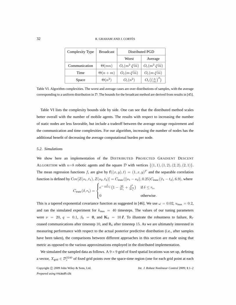
32 R. GRAHAM AND J. CORTES
Complexity Type Broadcast Distributed PGD
Worst Average
Communication Θ(mn) Oǫ(m2 d√
m) Oǫ(m2 d√
m)
Time Θ(n + m) Oǫ(m d√
m) Oǫ(m d√
m)
Space Θ(n2) Oǫ(n2) Oǫ
((
nm
)2)
Table VI. Algorithm complexities. The worst and average cases are over distributions of samples, with the average
corresponding to a uniform distribution inD. The bounds for the broadcast method are derived from results in [45].
Table VI lists the complexity bounds side by side. One can seethat the distributed method scales
better overall with the number of mobile agents. The resultswith respect to increasing the number
of static nodes are less favorable, but include a tradeoff between the average storage requirement and
the communication and time complexities. For our algorithm, increasing the number of nodes has the
additional benefit of decreasing the average computationalburden per node.
5.2. Simulations
We show here an implementation of the DISTRIBUTED PROJECTED GRADIENT DESCENT
ALGORITHM with n=8 robotic agents and the squareD with vertices(1, 1), (1, 2), (2, 2), (2, 1).
The mean regression functionsfi are give byf((x, y), t) = (1, x, y)T and the separable correlation
function is defined byCov[Z(s1, t1), Z(s2, t2)] = Ctrunc(‖s1 − s2‖, 0.25)Ctrunc(|t1 − t2|, 6.9), where
Ctrunc(δ, rs) =
e−δ
10∗rs(
1 − 3δ2rs
+ δ3
2r3s
)
if δ ≤ rs,
0 otherwise.
This is a tapered exponential covariance function as suggested in [46]. We useω = 0.02, umax = 0.2,
and ran the simulated experiment forkmax = 40 timesteps. The values of our tuning parameters
were ν = 20, q = 0.1, β0 = 0, and K0 = 10 I. To illustrate the robustness to failure, R7
ceased communications after timestep10, and R6 after timestep15. As we are ultimately interested in
measuring performance with respect to the actual posteriorpredictive distribution (i.e., after samples
have been taken), the comparisons between different approaches in this section are made using that
metric as opposed to the various approximations employed inthe distributed implementation.
We simulated the sampled data as follows. A9×9 grid of fixed spatial locations was set up, defining
a vector,Xgrid ∈ D3240e of fixed grid points over the space-time region (one for each grid point at each
Copyright c© 2009 John Wiley & Sons, Ltd. Int. J. Robust Nonlinear Control2009;1:1–2
Prepared usingrncauth.cls

COOPERATIVE ADAPTIVE SAMPLING OF RANDOM FIELDS WITH PARTIALLY KNOWN COVARIANCE 33
sampling timestep). A random vector was drawn from the jointprior distribution of all grid locations,
under the assumption thatσ2 andβ take their prior mean values, i.e., from the multivariate distribution,
Norm3240
(
F(Xgrid)T β0, σ
20K(Xgrid)
)
, whereσ20 =
qν
ν − 2
denotes the prior mean ofσ2. Each time a sample was taken by an agent, the value was determined
based on least squares (simple kriging) interpolation fromthis grid of fixed points. Figure 3 depicts
snapshots of the sample field used in the examples below. Notethat while the three consecutive
1 2
1
2
(a)
1 2
1
2
(b)
1 2
1
2
(c)
Figure 3. Snapshot of sample field over the square domain,D, for example problem at timesteps (a)k = 13, (b)
k = 14, and (c)k = 15.
timesteps depicted are not identical, there is clearly sometemporal correlation.
The DISTRIBUTED PROJECTEDGRADIENT DESCENTALGORITHM consists of a gradient descent
using an objective function defined by three basic approximations: the least squares approximation of
unrealized data; the approximate conditional variance based on regions defined by the static nodes;
and the approximate sigma mean based on blocks of samples to reduce the computational burden
over time. We begin by examining a centralized, computationally intensive implementation of the
gradient descent technique which uses only the least squares approximation. This allows us to compare
the (adaptive) gradient descent approach against two a priori approaches: a static configuration and
a lawnmower trajectory. The centralized implementation isexecuted by running the DISTRIBUTED
PROJECTEDGRADIENT DESCENTALGORITHM with one single static node (m = 1), responsible for
the whole predictive domain and using all samples up to stepk − 1 to estimateϕ at stepk. In the
language of Section 4.2, we lettblk=kmax. Each of the three approaches begins from the same initial
configuration, and the sample values are drawn from the same predetermined field as described above.
Copyright c© 2009 John Wiley & Sons, Ltd. Int. J. Robust Nonlinear Control2009;1:1–2
Prepared usingrncauth.cls
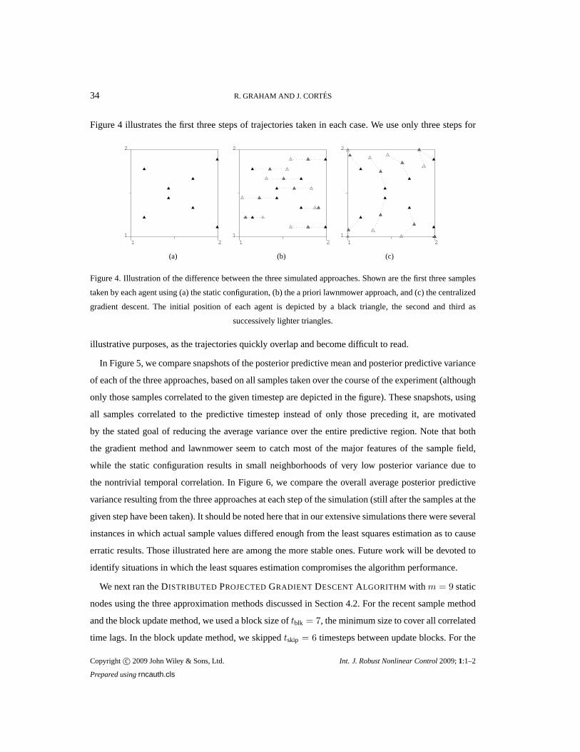
34 R. GRAHAM AND J. CORTES
Figure 4 illustrates the first three steps of trajectories taken in each case. We use only three steps for
1 21
2
(a)
1 21
2
(b)
1 21
2
(c)
Figure 4. Illustration of the difference between the three simulated approaches. Shown are the first three samples
taken by each agent using (a) the static configuration, (b) the a priori lawnmower approach, and (c) the centralized
gradient descent. The initial position of each agent is depicted by a black triangle, the second and third as
successively lighter triangles.
illustrative purposes, as the trajectories quickly overlap and become difficult to read.
In Figure 5, we compare snapshots of the posterior predictive mean and posterior predictive variance
of each of the three approaches, based on all samples taken over the course of the experiment (although
only those samples correlated to the given timestep are depicted in the figure). These snapshots, using
all samples correlated to the predictive timestep instead of only those preceding it, are motivated
by the stated goal of reducing the average variance over the entire predictive region. Note that both
the gradient method and lawnmower seem to catch most of the major features of the sample field,
while the static configuration results in small neighborhoods of very low posterior variance due to
the nontrivial temporal correlation. In Figure 6, we compare the overall average posterior predictive
variance resulting from the three approaches at each step ofthe simulation (still after the samples at the
given step have been taken). It should be noted here that in our extensive simulations there were several
instances in which actual sample values differed enough from the least squares estimation as to cause
erratic results. Those illustrated here are among the more stable ones. Future work will be devoted to
identify situations in which the least squares estimation compromises the algorithm performance.
We next ran the DISTRIBUTED PROJECTEDGRADIENT DESCENTALGORITHM with m = 9 static
nodes using the three approximation methods discussed in Section 4.2. For the recent sample method
and the block update method, we used a block size oftblk = 7, the minimum size to cover all correlated
time lags. In the block update method, we skippedtskip = 6 timesteps between update blocks. For the
Copyright c© 2009 John Wiley & Sons, Ltd. Int. J. Robust Nonlinear Control2009;1:1–2
Prepared usingrncauth.cls
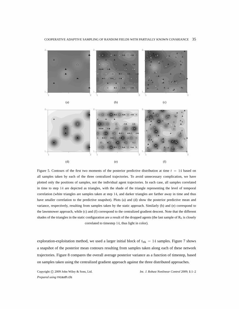
COOPERATIVE ADAPTIVE SAMPLING OF RANDOM FIELDS WITH PARTIALLY KNOWN COVARIANCE 35
1 2
1
2
(a)
1 2
1
2
(b)
1 2
1
2
(c)
1 2
1
2
(d)
1 2
1
2
(e)
1 2
1
2
(f)
Figure 5. Contours of the first two moments of the posterior predictive distribution at timet = 14 based on
all samples taken by each of the three centralized trajectories. To avoid unnecessary complication, we have
plotted only the positions of samples, not the individual agent trajectories.In each case, all samples correlated
in time to step14 are depicted as triangles, with the shade of the triangle representing the level of temporal
correlation (white triangles are samples taken at step14, and darker triangles are farther away in time and thus
have smaller correlation to the predictive snapshot). Plots (a) and (d) show the posterior predictive mean and
variance, respectively, resulting from samples taken by the static approach. Similarly (b) and (e) correspond to
the lawnmower approach, while (c) and (f) correspond to the centralized gradient descent. Note that the different
shades of the triangles in the static configuration are a result of the dropped agents (the last sample of R6 is closely
correlated to timestep14, thus light in color).
exploration-exploitation method, we used a larger initialblock of tblk = 14 samples. Figure 7 shows
a snapshot of the posterior mean contours resulting from samples taken along each of these network
trajectories. Figure 8 compares the overall average posterior variance as a function of timestep, based
on samples taken using the centralized gradient approach against the three distributed approaches.
Copyright c© 2009 John Wiley & Sons, Ltd. Int. J. Robust Nonlinear Control2009;1:1–2
Prepared usingrncauth.cls
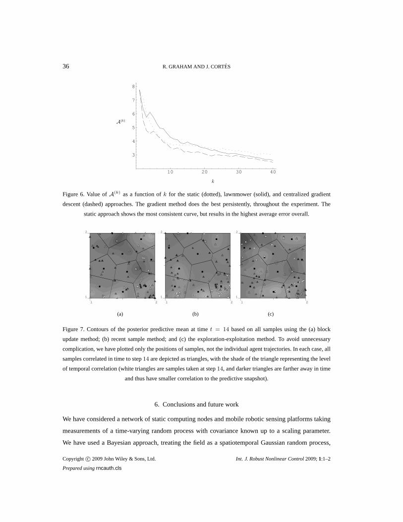
36 R. GRAHAM AND J. CORTES
10 20 30 40
3
4
5
6
7
8
k
A(k)
Figure 6. Value ofA(k) as a function ofk for the static (dotted), lawnmower (solid), and centralized gradient
descent (dashed) approaches. The gradient method does the bestpersistently, throughout the experiment. The
static approach shows the most consistent curve, but results in the highest average error overall.
1 2
1
2
(a)
1 2
1
2
(b)
1 2
1
2
(c)
Figure 7. Contours of the posterior predictive mean at timet = 14 based on all samples using the (a) block
update method; (b) recent sample method; and (c) the exploration-exploitation method. To avoid unnecessary
complication, we have plotted only the positions of samples, not the individual agent trajectories. In each case, all
samples correlated in time to step14 are depicted as triangles, with the shade of the triangle representing the level
of temporal correlation (white triangles are samples taken at step14, and darker triangles are farther away in time
and thus have smaller correlation to the predictive snapshot).
6. Conclusions and future work
We have considered a network of static computing nodes and mobile robotic sensing platforms taking
measurements of a time-varying random process with covariance known up to a scaling parameter.
We have used a Bayesian approach, treating the field as a spatiotemporal Gaussian random process,
Copyright c© 2009 John Wiley & Sons, Ltd. Int. J. Robust Nonlinear Control2009;1:1–2
Prepared usingrncauth.cls

COOPERATIVE ADAPTIVE SAMPLING OF RANDOM FIELDS WITH PARTIALLY KNOWN COVARIANCE 37
10 20 30 40
3
4
5
6
7
8
k
A(k)
Figure 8. Value ofA(k) as a function ofk using the centralized gradient method (solid), block update method
(dashed), recent sample method (dot-dash), and exploration-exploitation method (dotted). The three approximation
methods perform similarly to the centralized gradient method. The exploration-exploitation approach lags behind
at the end, while the two other approximation methods actually do better than thecentralized gradient approach.
and developed a novel approximation of the variance of the posterior predictive distribution which
may be calculated in a sequential and distributed fashion. Using this formulation, we have developed
a projected gradient descent algorithm which is distributed over the network of nodes and robots. We
have examined the complexity of this approach, and comparedit against the lower bound complexity
of a centralized “broadcast” method, showing that the distributed approach scales better with the
number of mobile agents. Future work will focus on theoretical guarantees on the accuracy of the
approximationA(k) and on the robustness to failure of the proposed algorithm. Guarantees on the
least squares approximation have proved extremely difficult, especially in the case of sparse samples.
Future work will also explore alternative methods, such as the expected value of the gradient of the
random field. The extension of these methods to networks in which the static agents are replaced by
slow moving ones would also be of interest. As mentioned in Remark 2.4, special care must be taken
to avoid singularities when generating local approximations for the universal kriging model. Rigorous
methods for handling this situation are also worth exploring.
7. Acknowledgments
The authors thank B. Sanso and H. Lee for several conversations on Bayesian spatial statistics. This
research was partially supported by NSF CAREER Award ECS-0546871.
Copyright c© 2009 John Wiley & Sons, Ltd. Int. J. Robust Nonlinear Control2009;1:1–2
Prepared usingrncauth.cls

38 R. GRAHAM AND J. CORTES
REFERENCES
1. Willcox JS, Bellingham JG, Zhang Y, Baggeroer AB. Performance metrics for oceanographic surveys with autonomous
underwater vehicles.IEEE Journal of Oceanic Engineering2001;26(4):711–725.
2. Handcock MS, Wallis JR. An approach to statistical spatial-temporal modeling of meteorological fields.Journal of the
American Statistical Association1994;89(426):368–378.
3. Higdon D. A process-convolution approach to modelling temperatures in the north atlantic ocean.Environmental and
Ecological Statistics1998;5:173–190.
4. Gaudard M, Karvson M, Linder E, Sinha D. Bayesian spatial prediction.Environmental and Ecological Statistics1999;
6:147–171.
5. Lee ND, Zidek JV.Statistical Analysis of Environmental Space-Time Processes. Springer Series in Statistics, Springer:
New York, 2006.
6. Chaloner K, Verdinelli I. Bayesian experimental design, areview.Statistical Science1995;10(3):273–304.
7. Pukelsheim F.Optimal Design of Experiments, Classics in Applied Mathematics, vol. 50. SIAM: Philadelphia, PA, 2006.
8. Liski EP, Mandal NK, Shah KR, Sinha BK.Topics in Optimal Design, Lecture Notes in Statistics, vol. 163. Springer: New
York, 2002.
9. Popa DO, Sreenath K, Lewis FL. Robotic deployment for environmental sampling applications.International Conference
on Control and Automation, Budapest, Hungary, 2005; 197–202.
10. MacKay DJC. Information-based objective functions for active data selection.Neural Computation1992;4(4):590–604.
11. Gramacy RB. Bayesian treed Gaussian process models. PhD Thesis, University of California, Santa Cruz, CA 95064
December 2005. Department of Applied Math & Statistics.
12. Caselton WF, Zidek JV. Optimal monitoring network designs.Statistics & Probability Letters1984;2(4):223–227.
13. Krause A, Singh A, Guestrin C. Near-optimal sensor placements in Gaussian processes: Theory, efficient algorithms and
empirical studies.Journal of Machine Learning Research2008;9:235–284.
14. Singh A, Krause A, Guestrin C, Kaiser WJ. Efficient informative sensing using multiple robots.Journal of Artificial
Intelligence Research2009;34:707–755.
15. Leonard NE, Paley D, Lekien F, Sepulchre R, Fratantoni DM, Davis R. Collective motion, sensor networks and ocean
sampling.Proceedings of the IEEE2007;95(1):48–74.
16. Zhang F, Fiorelli E, Leonard NE. Exploring scalar fields using multiple sensor platforms: tracking level curves.IEEE Conf.
on Decision and Control, New Orleans, LA, 2007; 3579–3584.
17. Cortes J. Distributed Kriged Kalman filter for spatial estimation.IEEE Transactions on Automatic Control2009;
54(12):2816–2827.
18. Lynch KM, Schwartz IB, Yang P, Freeman RA. Decentralized environmental modeling by mobile sensor networks.IEEE
Transactions on Robotics2008;24(3):710–724.
19. Martınez S. Distributed interpolation schemes for field estimation by mobile sensor networks.IEEE Transactions on
Control Systems Technology2010;18(2):491–500.
20. Demetriou MA, Hussein II. Estimation of spatially distributed processes using mobile spatially distributed sensor network.
SIAM Journal on Control and Optimization2009;48(1):266–291.
21. Hoffmann GM, Tomlin CJ. Mobile sensor network control using mutual information methods and particle filters.IEEE
Transactions on Automatic Control2010;55(1):32–47.
22. Ucinski D. Optimal Measurement Methods for Distributed Parameter System Identification. CRC Press, 2005, doi:
Copyright c© 2009 John Wiley & Sons, Ltd. Int. J. Robust Nonlinear Control2009;1:1–2
Prepared usingrncauth.cls

COOPERATIVE ADAPTIVE SAMPLING OF RANDOM FIELDS WITH PARTIALLY KNOWN COVARIANCE 39
10.1201/9780203026786.fmatt.
23. Berke O. On spatiotemporal prediction for on-line monitoring data.Communications in Statistics - Theory and Methods
1998;27(9):2343–2369.
24. Mardia KV, Goodall C, Redfern EJ, Alonso FJ. The Kriged Kalman filter.Test1998;7(2):217–285. With discussion.
25. Kitanidis PK. Parameter uncertainty in estimation of spatial functions: Bayesian analysis.Water Resources Research1986;
22:449–507.
26. Wiens DP. Robustness in spatial studies I: minimax prediction and II: minimax design.Environmetrics2005;16:191–203
and 205–217.
27. Sutton RS, Barto AG.Reinforcement Learning: An Introduction. MIT Press, 1998.
28. Krause A, Guestrin C. Nonmyopic active learning of Gaussian processes: an exploration-exploitation approach.
International Conference on Machine Learning, Corvallis, OR, 2007.
29. Graham R, Cortes J. A cooperative deployment strategy for optimal sampling inspatiotemporal estimation.IEEE Conf. on
Decision and Control, Cancun, Mexico, 2008; 2432–2437.
30. Graham R, Cortes J. Distributed sampling of random fields with unknown covariance.American Control Conference, St.
Louis, MO, 2009; 4543–4548.
31. Bertsekas DP. On the Goldstein-Levitin-Polyak gradient projection method.IEEE Transactions on Automatic Control1976;
21(2):174–184.
32. Leonard T, Hsu JSJ.Bayesian Methods, Cambridge series in statistical and probabilistic mathematics, vol. 1. Cambridge
University Press: Cambridge, UK, 1999.
33. Gottschalk L. Interpolation of runoff applying objective methods.Stochastic Hydrology and Hydraulics1993;7:269–281.
34. Wackernagel H.Multivariate Geostatistics. 3rd edn., Springer: New York, 2006.
35. Robert CP, Casella G.Monte Carlo statistical methods. Springer texts in statistics, Springer: New York, 2004.
36. Bertsekas DP, Tsitsiklis JN.Parallel and Distributed Computation: Numerical Methods. Athena Scientific, 1997.
37. Olfati-Saber R, Murray RM. Consensus problems in networks of agents with switching topology and time-delays.IEEE
Transactions on Automatic Control2004;49(9):1520–1533.
38. Bullo F, Cortes J, Martınez S.Distributed Control of Robotic Networks. Applied Mathematics Series, Princeton University
Press, 2009. Electronically available at http://coordinationbook.info.
39. Lynch NA.Distributed Algorithms. Morgan Kaufmann, 1997.
40. Cormen TH, Leiserson CE, Rivest RL, Stein C.Introduction to Algorithms. 2 edn., MIT Press, 2001.
41. Carle J, Myoupo JF. Topological properties and optimal routing algorithms for three dimensional hexagonal grid networks.
High performance computing in the Asia-Pacific region, 2000; 116–121.
42. Chen MS, Shin KG, Kandlur DD. Addressing, routing, and broadcasting in hexagonal mesh multiprocessors.IEEE
Transactions on Computersjan 1990;39(1):10–18.
43. Okabe A, Boots B, Sugihara K, Chiu SN.Spatial Tessellations: Concepts and Applications of Voronoi Diagrams. 2 edn.,
Wiley Series in Probability and Statistics, Wiley, 2000.
44. Mohar B. The Laplacian spectrum of graphs.Graph Theory, Combinatorics, and Applications, vol. 2, Alavi Y, Chartrand
G, Oellermann OR, Schwenk AJ (eds.). Wiley, 1991; 871–898.
45. Topkis DM. Concurrent broadcast for information dissemination. IEEE Transactions on Software Engineeringoct 1985;
SE-11(10):1107–1112.
46. Furrer R, Genton MG, Nychka D. Covariance tapering for interpolation of large spatial datasets.Journal of Computational
and Graphical Statistics2006;15(3):502–523.
Copyright c© 2009 John Wiley & Sons, Ltd. Int. J. Robust Nonlinear Control2009;1:1–2
Prepared usingrncauth.cls

40 R. GRAHAM AND J. CORTES
47. Bernstein DS.Matrix Mathematics. Princeton University Press: Princeton, NJ, 2005.
48. Henderson HV, Searle SR. On deriving the inverse of a sum of matrices.SIAM Review1981;23(1):53–60.
49. Udwadia FE. Some convergence results related to the JOR iterative method for symmetric, positive-definite matrices.
Applied Mathematics and Computation1992;47(1):37–45.
APPENDIX
I. Predictions with a subset of measurements
We present here a series of results concerning the relationship between subsets of spatiotemporal
sample locations and hypothetical predictions made from partial information. LetY ∈ Rn denote
a full set of measurements at locationsX ∈ Dne . Let n1, n2 ∈ Z>0 such thatn1 + n2 = n. Consider a
partition of the measurementsY = (Y1, Y2) such thatY1 ∈ Rn1 andY2 ∈ R
n2 , and a similar partition
of X. Note that due to the invariance ofϕ andφ under permutations of the samples, our discussion is
valid for any partition of the measurements, not necessarily restricted to samples that are sequential in
time. We will useK1, respectivelyK2, to denote the correlation matrix of locationsX1, respectively
X2, and analogous notation for the matricesF1,F2,E1,E2. Let K12 = KT21 ∈ R
n1×n2 denote the
matrix of cross-correlation between the two location vectors.
We begin with a multivariate version of the posterior predictive variance from Proposition 2.1, which
can be considered the hypothetical distribution of the measurements at space-time locationsX2 given
the samplesY1. This result can be obtained by applying Bayes Theorem to theprior model.
Lemma I.1 (Multivariate posterior predictive distribution) Under the Bayesian model(2), the
multivariate posterior predictive distribution of hypothetical samplesY2 conditional on dataY1 is
then2-variate shifted Students t distribution withν + n1 degrees of freedom, which takes the form,
p(Y2|Y1) ∝ det Var[Y2|Y1]− 1
2
(
1 +(Y2 − E[Y2|Y1])
TVar[Y2|Y1]
−1 (Y2 − E[Y2|Y1])
ν + n1 − 2
)−ν+n1+n2
2
.
Here, the expectation is given by
E[Y2|Y1] = ξT2|1(E1 + K
−10 )−1
(
F1K−11 Y1 + K
−10 β0
)
+ K21K−11 Y1,
whereξ2|1 = F2 − F1K−11 K12. The covariance matrix is given by
Var[Y2|Y1] = ϕ(Y1,X1)φ(X2;X1),
where, with a slight abuse of notation, we have usedφ(X2;X1) to denote the following multivariate
Copyright c© 2009 John Wiley & Sons, Ltd. Int. J. Robust Nonlinear Control2009;1:1–2
Prepared usingrncauth.cls

COOPERATIVE ADAPTIVE SAMPLING OF RANDOM FIELDS WITH PARTIALLY KNOWN COVARIANCE 41
extensions ofφ andϕ,
φ(X2;X1) = K2 − K21K−11 K12 + ξT
2|1
(
K−10 + E1
)−1ξ2|1,
ϕ(Y1,X1) =1
ν + n1 − 2
(
qν +(
Y1 − FT1 β0
)T (K1 + F
TK0F
)−1 (Y1 − F
T1 β0
)
)
.
In the sequel, we will find useful the matricesM ∈ R(n+p)×(n+p) andM2 ∈ R
(n2+p)×(n2+p) and
vectorsU ∈ Rn+p andU2 ∈ R
n2+p defined as,
M =
K FT
F −K−10
, U =
Y
−K−10 β0
, M2 =
K2 FT2
F2 −K−10
, U2 =
Y2
−K−10 β0
.
Note thatM2 is the lower right submatrix ofM under a different partition, andU2 is the corresponding
subvector ofU . It can be shown that the matricesM andM2 are invertible.
Proposition I.2 (Approximate conditional variance) The termφ(x0;X) may be written in terms of
spatiotemporal locationsX2 as,
φ(x0;X) = φ(x0;X2) − (k1 − µ1)T
φ(X1;X2)−1 (k1 − µ1) , where
µ1 =
K21
F1
T
M−12
k2
f(x0)
, k1 = Cor[Z(x0), Y1], k2 = Cor[Z(x0), Y2].
Thereforeφ(x0;X) ≤ φ(x0;X2) with equality if and only ifk1 = µ1.
Proof. First, we note that the conditional variance can be written usingM as,
φ(x0;X) = Cor[Z,Z] −
k
f(x0)
T
M−1
k
f(x0)
.
Next, we point out that with the proper partitioning ofM, the matrix φ(X1;X2) is the Schur
Complement,(M2 |M ). Using this, and a similar partition of the vectork, one arrives at the result.
The following result illustrates a number of ways in which the sigma mean may be restated.
Lemma I.3 (Restated sigma mean) The quadratic formUTM−1U can be expressed as,
UTM−1U = (Y − FT β0)
T (K + FTK0F)−1(Y − F
T β0) − βT0 K
−10 β0 (9a)
= Y TK
−1Y −(
K−10 β0 + FK
−1Y)T (
K−10 + E
)−1(K
−10 β0 + FK
−1Y)
(9b)
= UT2 M−1
2 U2 + (Y1 − E[Y1|Y2])T φ(X1;X2)
−1(Y1 − E[Y1|Y2]). (9c)
Furthermore, the termϕ(Y,X) may be written as,
ϕ(Y,X) =qν + βT
0 K−10 β0 + UTM−1U
ν + n − 2. (10)
Copyright c© 2009 John Wiley & Sons, Ltd. Int. J. Robust Nonlinear Control2009;1:1–2
Prepared usingrncauth.cls

42 R. GRAHAM AND J. CORTES
Proof. Each of the three representations of the quadratic form may be derived directly by using [47,
Proposition 2.8.7] to expand the inverse matrix onto Schur complements. Plugging representation (9a)
into (10) yields the form given in Proposition 2.1.
The generalized least squares (GLS) approximation arises naturally from partitioning the elements
of the termK−1Y . The following lemma gives explicit form in terms of the GLS error.
Lemma I.4 (Generalized least squares approximations) Let YLS = K21K−11 Y1 be the generalized
least squares estimate ofY2 based on samplesY1 (conditional on all parameters), and letyLS =
Y2 − YLS. Then we can write,
K−1Y =
K−11 Y1
0
+
−K−11 K12 (K1 |K )
−1yLS
(K1 |K )−1
yLS
. (11)
Proof of Proposition 4.3. Using (11) in Lemma I.4 we write,
Y TK
−1Y = Y T1 K
−11 Y1 + (Y2 − YLS)T (K1 |K ) (Y2 − YLS)
FK−1Y = F
T1 K
−11 Y1 + ξ2|1 (K1 |K ) (Y2 − YLS).
Here we have used the simpler indexed notation,Y1 = Y (1:k) andY2 = Y (k+1) to simplify the algebra.
Applying these results to (9b) in Lemma I.3 yields,
UTM−1U = Y T1 K
−11 Y1 − (K−1
0 β0 + F1K−11 Y1)
T (K−10 + E)−1(K−1
0 β0 + F1K−11 Y1)
+ (Y2 − YLS)T (K1 |K )−1
(Y2 − YLS)
− 2(K−10 β0 + F1K
−11 Y1)
T (K−10 + E)−1(ξ2|1 (K1 |K )
−1(Y2 − YLS))
− (ξ2|1 (K1 |K )−1
(Y2 − YLS))T (K−10 + E)−1(ξ2|1 (K1 |K )
−1(Y2 − YLS)).
Using, e.g. [48, Equation (12,17)], we can write,
φ(X2;X1) = (K1 |K )−1
+ (K1 |K )−1
ξT2|1(K
−10 + E)−1ξ2|1 (K1 |K )
−1.
With some algebraic manipulation we arrive at the result,
UTM−1U = Y T1 K
−11 Y1 − (K−1
0 β0 + F1K−11 Y1)
T (K−10 + E)−1(K−1
0 β0 + F1K−11 Y1)
+ (yLS − 2µ2|1)φ(X2;X1)−1yLS.
The result follows from Lemma I.3.
Copyright c© 2009 John Wiley & Sons, Ltd. Int. J. Robust Nonlinear Control2009;1:1–2
Prepared usingrncauth.cls

COOPERATIVE ADAPTIVE SAMPLING OF RANDOM FIELDS WITH PARTIALLY KNOWN COVARIANCE 43
II. Near optimal relaxation parameter for JOR
Here we present some results regarding a relaxation parameter for the JOR algorithm which is nearly
optimal with respect to the rate of convergence of the algorithm for a certain class of matrices.
Specifically we are interested in the class of symmetric, positive definite matricesC with ones on
the diagonal. Lety(t) = (y1(t), . . . , yn(t))T ∈ Rn be the vector updated during the JOR iteration
in (5). Lete(t) = ‖C−1b − y(t)‖ denote the error at iterationt. We may write,
e(t) ≤ (ρ(I − hC))te(0), (12)
giving a bound on the error at stept based on the initial error. The value ofρ(I−hC) therefore controls
the rate of convergence, and choosing the relaxation parameter,h, is of vital importance. Throughout
this section we will use the shorthandλmax = λmax(C) andλmin = λmin(C). The work [49] provides
results concerning the convergence of the JOR algorithm, including an optimal relaxation parameter,
which in our case is equivalent tohopt =2
λmax+λmin. In this section we will introduce an approximation
to this optimal value which may be calculated in a distributed manner.
Proposition II.1. Assume thatC ∈ Rn×n is a symmetric positive definite matrix with all diagonal
entries equal to1. Let β and α denote the maximum off-diagonal entry ofC and the maximum off-
diagonal row sum ofC, respectively,
β = maxi6=j∈1,...,n
cij ≥ 0, α = maxi∈1,...,n
n∑
j=1j 6=i
cij
≥ 0.
Leth∗ = 22+α−β . Then usingh∗ as the relaxation parameter in the JOR algorithm to solvey = C−1b
results in guaranteed convergence.
Proof. Recall from Section 2.3 that convergence of the JOR algorithm is guaranteed as long
as h∗ ∈(
0, 2λmax
)
. This can also be seen from (12), sinceh outside of this range would yield
ρ(I − hC) > 1. SinceC is symmetric positive definite with1’s on the diagonal, all off-diagonal
entries must have magnitude strictly less than1. Thus1 − β > 0. The Gershgorin circle theorem
(e.g. [47, Fact 4.10.13]) implies thatλmax ≤ 1+α. Together, these two results yield2+α−β > λmax,
which implies that 22+α−β < 2
λmax, and the result follows.
Lemma II.2. Under the assumptions of Proposition II.1,h∗ ≤ 1λmin
, with equality if and only ifC is
then × n identity matrix.
Copyright c© 2009 John Wiley & Sons, Ltd. Int. J. Robust Nonlinear Control2009;1:1–2
Prepared usingrncauth.cls

44 R. GRAHAM AND J. CORTES
Proof. First, note the following implication chain,
λmin ≤ 1 =⇒ 2λmin ≤ 2 + α − β =⇒ h∗ ≤ 1
λmin.
Now, assume thath∗ = 1λmin
. This implies thatλmin = 1 + α − β, but λmin ≤ 1, andα ≥ β. So we
must haveλmin = 1. Since the diagonal entries ofC are all1, the smallest eigenvalue can only be1 if
all off-diagonal entries are zero, i.e., ifC = In.
Lemma II.3. Under the assumptions of Proposition II.1,|1 − h∗λmin| ≥ |1 − h∗λmax|.
Proof. Using Lemma II.2, we have|1 − h∗λmin| = 1 − h∗λmin. The result may then be shown by
two separate cases. First, note that ifh∗ ≤ 1λmax
then we have,
|1 − h∗λmax| = 1 − h∗λmax ≤ |1 − h∗λmin|,
so the result holds in this case. For the second case, assume that h∗ > 1λmax
. Then |1 − h∗λmax| =
h∗λmax − 1. The inclusion principle and the fact thatC is positive definite give us the bounds
0 < λmin ≤ 1 − α. Combined with the previously mentioned Gershgorin bound,λmax ≤ 1 + α,
this allows us to write,
λmax + λmin
2 + α − β≤ 1, 2
λmax + λmin
2 + α − β≤ 2,
h∗ (λmax + λmin) ≤ 2, h∗λmax− 1 ≤ 1 − h∗λmin.
Thus in all cases,|1 − h∗λmax| ≤ |1 − h∗λmin|.
Proposition II.4. Under the assumptions of Proposition II.1, further assume thatλmin ≥ λ for some
λ ∈ (0, 1). Then0 ≤ ρ(I − h∗C) < 1 − 2λ
2+α−β
Proof. First note that the spectral radius is given bymax |1 − h∗λmin|, |1 − h∗λmax|, and is clearly
nonnegative. From Lemma II.3, we haveρ(I − h∗C) = |1 − h∗λmin|. From Lemma II.2, we can infer
ρ(I − h∗C) = 1 − h∗λmin. The upper bound follows by comparing1 − h∗λmin against1 − h∗λ.
Copyright c© 2009 John Wiley & Sons, Ltd. Int. J. Robust Nonlinear Control2009;1:1–2
Prepared usingrncauth.cls


![User-Independent Motion State Recognition Using Smartphone ... · random fields (CRFs) to recognize concurrent and interleaving activities. Liao et al. [19] applied hierarchical](https://static.fdocuments.us/doc/165x107/60e78c0d97bd6c50a55e33a7/user-independent-motion-state-recognition-using-smartphone-random-ields-crfs.jpg)